Abelian sandpile model and Biggs-Merino polynomial for directed graphs

Abstract.

We prove several results concerning a polynomial that arises from the sandpile model on directed graphs; these results are previously only known for undirected graphs. Implicit in the sandpile model is the choice of a sink vertex, and it is conjectured by Perrot and Pham that the polynomial $c_{0}+c_{1}y+\ldots c_{n}y^{n}$, where $c_{i}$ is the number of recurrent classes of the sandpile model with level $i$, is independent of the choice of the sink. We prove their conjecture by expressing the polynomial as an invariant of the sinkless sandpile model. We then present a bijection between arborescences of directed graphs and reverse $G$-parking functions that preserves external activity by generalizing Cori-Le Borgne bijection for undirected graphs. As an application of this bijection, we extend Merino’s Theorem by showing that for Eulerian directed graphs the polynomial $c_{0}+c_{1}y+\ldots c_{n}y^{n}$ is equal to the greedoid polynomial of the graph.

1. Introduction

To what extent do the known results for undirected graphs extend to directed graphs? Driven by this question, we consider a remarkable theorem of Merino López [ML97] that expresses a one variable specialization of the Tutte polynomial of an undirected graph in terms of the abelian sandpile model on the graph. In this paper, we show that this theorem can be extended to all Eulerian directed graphs, and a weaker version of the theorem can be extended to all directed graphs.

The abelian sandpile model is a dynamical system on a finite directed graph that starts with a number of chips at each vertex of the graph. If a vertex has at least as many chips as its outgoing edges, then we are allowed to fire the vertex by sending one chip along each edge leaving the vertex to the neighbors of the vertex. This model was introduced by Dhar [Dha90] as a model to study the concept of self-organized criticality introduced in [BTW88]. Since then it has been studied in several different field of mathematics. In graph theory it was studied under the name of chip-firing game [Tar88, BLS91]; it appears in arithmetic geometry in the study of the Jacobian of algebraic curves [Lor89, BN07]; and in algebraic graph theory it relates to the study of potential theory on graphs [Big97b, BS13].

It is common to study the sandpile model by specifying a vertex as the sink vertex, and all chips that end up at the sink vertex are removed from the process. For a strongly connected directed graph, this guarantees that the sandpile model terminates (i.e. when none of the vertices have enough chips to be fired) in finite time. After fixing a sink, one can study a special type of chip configurations with the following property. A chip configuration is recurrent if, for any arbitrary chip configuration as the initial state, one can add a finite amount of chips to each vertex so that the recurrent configuration is the state of the sandpile model when the process terminates.

It was conjectured by Biggs [Big97a] and was proved by Merino López [ML97] that, for any undirected graph $G$ and any choice of the sink vertex $s$,

$$c_{0}+c_{1}y+\ldots+c_{n}y^{n}=y^{|E(G)|}\mathcal{T}(G;1,y)\qquad\text{(Merino's Theorem)},$$

where $\mathcal{T}(G;x,y)$ is the Tutte polynomial of the graph and $c_{i}$ is the number of recurrent configurations with $i-\deg(s)$ chips. (We remark that the extra factor $y^{|E(G)|}$ does not appear in the right side of [ML97, Theorem 3.6] as their left side differs from ours by the same factor.) As the Tutte polynomial is defined without any involvement of the vertex $s$, this implies that $c_{0}+c_{1}y+\ldots+c_{n}y^{n}$ does not depend on the choice of $s$.

The sink independence of the polynomial $c_{0}+c_{1}y+\ldots+c_{n}y^{n}$ was then extended to all Eulerian directed graphs by Perrot and Pham [PP16], and they observed that the same statement does not hold for non-Eulerian directed graphs. However, they conjectured that a variant of this polynomial has the sink independence property for all directed graphs.

Perrot and Pham defined an equivalence relation on the recurrent configurations (Definition 3.3), and they defined the total number of chips of an equivalence class to be the maximum of the total number of chips of configurations contained in the class. The conjecture of Perrot and Pham is that the sink independence property is true for the polynomial,

$$\mathcal{B}(G,s;y):=c_{0}^{\prime}+c_{1}^{\prime}y+\ldots+c_{n}^{\prime}y^{n},$$

where $c_{i}$ is the number of equivalence classes with $i-\operatorname{\textnormal{outdeg}}(s)$ chips. We prove their conjecture by expressing $\mathcal{B}(G,s;y)$ as an invariant of the sinkless sandpile model (which, as its name implies, does not involve any choice of sink vertex).

Theorem 1.1 (Weak version of Merino’s theorem [PP16, Conjecture 1]).

Let $G$ be a strongly connected digraph. Then the polynomial $\mathcal{B}(G,s;y)$ is independent of the choice of the vertex $s$.

We call $\mathcal{B}(G,s;y)$ the Biggs-Merino polynomial to honor the contribution of Biggs and Merino López to this subject.

One consequence of Merino’s Theorem is that, for any undirected graph and for any $i$, the number of recurrent configurations with $i-\deg(s)$ chips is equal to the number of spanning trees with external activity $i$. A bijective proof of this statement was given by Cori and Le Borgne [CLB03], and we generalize the bijection of Cori and Le Borgne to all Eulerian directed graphs.

Let $G$ be a strongly connected digraph, and let $s$ be a vertex of $G$. A reverse $G$-parking function [PS04] with respect to $s$ is a function $f:V(G)\setminus\{s\}\to\mathbb{N}_{0}$ such that, for any non-empty subset $A\subseteq V(G)\setminus\{s\}$, there exists $v\in A$ for which $f(v)$ is strictly smaller than the number of edges from $V(G)\setminus A$ to $v$. An arborescence of $G$ rooted at $s$ is a subgraph of $G$ that contains $|V(G)|-1$ edges and such that for any vertex $v$ of $G$ there exists a unique directed path from $s$ to $v$ in the subgraph.

We show that Cori-Le Borgne bijection generalizes to a bijection between reverse $G$-parking functions and arborescences of $G$ for all directed graphs. For the full description of the bijection, see Algorithm 1.

Theorem 1.2.

Let $G$ be a strongly connected digraph, and let $s\in V(G)$. Then Cori-Le Borgne bijection generalizes to a bijection that sends reverse $G$-parking functions with respect to $s$ to arborescences of $G$ rooted at $s$. Furthermore, the external activity of the output arborescence is the level of the input reverse $G$-parking function.

The external activity of an arborescence and the level of a $G$-parking function are defined in Definition 5.2 and Definition 5.6, respectively.

As a consequence of Theorem 1.2 and the duality between reverse $G$-parking functions and recurrent configurations for Eulerian directed graphs [HLM⁺08, Theorem 4.4], we get the extension of Merino’s Theorem for Eulerian directed graphs.

Theorem 1.3 (Merino’s Theorem for Eulerian directed graphs).

Let $G$ be a connected Eulerian digraph. Then for any $s\in V(G)$,

$$c_{0}+c_{1}y+\ldots+c_{n}y^{n}=t_{0}+t_{1}y+\ldots+t_{n}y^{n},$$

where $c_{i}$ is the number of recurrent configurations with $i-\operatorname{\textnormal{outdeg}}(s)$ chips and $t_{i}$ is the number of arborescences of $G$ rooted at $s$ with external activity $i$.

The right side of Theorem 3.7 is known in the literature as the greedoid polynomial [BKL85], and it can be considered as a single variable generalization of the Tutte polynomial for directed graphs [GM89, GT90, GM01].

This paper is arranged as follows: In Section 2 we give a review on the sinkless sandpile model and the sandpile model with a sink. In Section 3 we prove Theorem 1.1. In Section 4 we prove a recurrence relation for the Biggs-Merino polynomial. In Section 5 we prove Theorem 1.2 and Theorem 1.3. Finally in Section 6 we include a list of questions for future research.

2. Review of abelian sandpile models

In this section we review basic results concerning the sinkless sandpile model and the sandpile model with a sink. We refer to [BL92, HLM⁺08] for a more detailed introduction of these two models, to [PPW13] for an algebraic treatment of this model, and to [BL16a, BL16b, BL16c] for a generalization of these models.

We use $G:=(V(G),E(G))$ to denote a directed graph (digraph for short), possibly with loops and multiple edges. We use $V$ and $E$ as a shorthand for $V(G)$ and $E(G)$ when the digraph $G$ is evident from the context. Each edge $e\in E$ is directed from its source vertex to its target vertex. The outdegree of a vertex $v\in V$, denoted by $\operatorname{\textnormal{outdeg}}(v)$, is the number of edges with $v$ as source vertex, while the indegree of a vertex $v\in V$, denoted by $\operatorname{\textnormal{indeg}}(v)$, is the number of edges with $v$ as target vertex.

In this paper, we identify an undirected graph $G$ with the directed graph obtained by replacing each undirected edge $e:=\{i,j\}$ of $G$ with two directed edges $(i,j)$ and $(j,i)$. A digraph obtained in this way is called bidirected.

A digraph $G$ is Eulerian if $\operatorname{\textnormal{outdeg}}(v)=\operatorname{\textnormal{indeg}}(v)$ for all $v\in V$. In particular, all bidirected graphs are Eulerian. A digraph is strongly connected if for any two vertices $v,w\in V$ there exists a directed path from $v$ to $w$. Note that a connected Eulerian digraph is always strongly connected. Throughout this paper, we always assume that our digraph $G$ is strongly connected.

The Laplacian matrix $\Delta$ of a digraph $G$ is the square matrix $(\Delta_{i,j})_{V\times V}$ given by:

$$\Delta_{i,j}:=\begin{cases}\operatorname{\textnormal{outdeg}}(i)-\#\text{ of loops in vertex }i&\text{ if }i=j;\\ -\text{ the number of of edges from vertex }j\text{ to vertex }i&\text{ if }i\neq j.\end{cases}$$

Note that the Laplacian matrix is a symmetric matrix if and only if $G$ is bidirected.

Definition 2.1 (Primitive period vector).

A vector $\mathbf{r}\in\mathbb{R}^{V}$ is a period vector of $G$ if it is non-negative, integral, and $\mathbf{r}\in\ker(\Delta)$. A period vector is primitive if its entries has no non-trivial common divisor. ∎

If $G$ is a strongly connected digraph, then a primitive period vector exists, is unique, and is strictly positive [BL92, Proposition 4.1(i)]. Throughout this paper, we will use $\mathbf{r}$ to denote the primitive period vector of $G$.

Note that any nonzero period vector of $G$ is a positive multiple of the primitive period vector [BL92, Proposition 4.1(iii)]. Also note that the primitive period vector is equal to $(1,\ldots,1)$ if and only if $G$ is an Eulerian digraph [BL92, Proposition 4.1(ii)].

A reverse arborescence of $G$ rooted at $v\in V$ is a subgraph $G$ that contains $|V|-1$ edges and such that for any $w\in V$ there exists a unique directed path from $w$ to $v$ in the subgraph. Let $t_{v}$ denote the number of reverse arborescences of $G$ rooted at $v$. Note that $t_{v}>0$ for all $v\in V$ if $G$ is strongly connected.

Definition 2.2 (Period constant).

The period constant $\alpha$ of a strongly connected digraph $G$ is

$$\alpha:=\underset{v\in V}{\gcd}\,\{t_{v}\}.\qed$$

If $G$ is strongly connected, then by the markov chain tree theorem [AT89] the primitive period vector $\mathbf{r}$ is given by

$$\mathbf{r}(v)=\frac{t_{v}}{\alpha}\quad(v\in V).$$

2.1. Sinkless abelian sandpile model

The sinkless (abelian) sandpile model on a strongly connected digraph $G$, denoted by $\textnormal{Sand}(G)$, starts with a number of chips at each vertex of $G$. A sinkless (chip) configuration $\mathbf{c}$ is a vector in $\mathbb{N}_{0}^{V}$, with $\mathbf{c}(v)$ representing the number of chips in the $v\in V$. A sinkless firing move on $\mathbf{c}$ consists of removing $\operatorname{\textnormal{outdeg}}(v)$ chips from a vertex $v$ and sending each of those chips along each edge leaving $v$ to a neighbor of $v$. Denote by $\textbf{{1}}_{v}$ the vector in $\mathbb{N}_{0}^{V}$ given by $\textbf{{1}}_{v}(v):=1$ and $\textbf{{1}}_{v}(w):=0$ for all $w\in V\setminus\{v\}$. Note that a sinkless firing move changes a sinkless configuration $\mathbf{c}$ to $\mathbf{c}-\Delta\textbf{{1}}_{v}$.

Note that the result of a sinkless firing move is not necessarily a sinkless configuration, as the $v$-th entry of $\mathbf{c}-\Delta\textbf{{1}}_{v}$ is negative if $\mathbf{c}(v)\leq\operatorname{\textnormal{outdeg}}(v)$. A sinkless firing move is legal if the fired vertex has at least as many chips as its outgoing edges, or equivalently if the result of the firing move is another sinkless configuration. A sinkless configuration $\mathbf{c}$ is stable if $\mathbf{c}(v)<\operatorname{\textnormal{outdeg}}(v)$ for all $v\in V$, or equivalently if there are no legal sinkless firing moves for $\mathbf{c}$.

Each finite (possibly empty) sequence of sinkless firing moves is associated with an odometer $\mathbf{q}\in\mathbb{N}_{0}^{V}$, where $\mathbf{q}(v)$ is equal to the number of times the vertex $v$ is being fired in the sequence. Note that applying a finite sequence of firing moves with odometer $\mathbf{q}$ to a sinkless configuration $\mathbf{c}$ gives us the sinkless configuration $\mathbf{c}-\Delta\mathbf{q}$.

For any two sinkless configurations $\mathbf{c},\mathbf{d}$ of $G$, we write $\mathbf{c}\longrightarrow\mathbf{d}$ if there exists a finite (possibly empty) sequence of legal sinkless firing moves that sends $\mathbf{c}$ to $\mathbf{d}$. If the odometer $\mathbf{q}$ of the sequence is known, we will write $\mathbf{c}\xlongrightarrow[\mathbf{q}]{}\mathbf{d}$ instead.

It follows from the definition that $\longrightarrow$ is a transitive relation.

Definition 2.3 (Recurrent sinkless configurations).

Let $G$ be a strongly connected digraph. A sinkless configuration $\mathbf{c}$ of $G$ is (sinkless) recurrent if it satisfies these two conditions:

• The configuration $\mathbf{c}$ is not stable; and

• If $\mathbf{d}$ is a sinkless configuration that satisfies $\mathbf{c}\longrightarrow\mathbf{d}$, then $\mathbf{d}\longrightarrow\mathbf{c}$. ∎

We use $\textnormal{Rec}(G)$ to denote the set of all recurrent sinkless configurations of $G$.

Recall that $\mathbf{r}$ denote the primitive period vector of $G$.

Lemma 2.4 ([BL92, Lemma 1.3, Lemma 4.3]).

Let $G$ be a strongly connected digraph.

1. If $\mathbf{q}_{1},\mathbf{q}_{2}\in\mathbb{N}_{0}^{V}$ satisfy $\mathbf{q}_{1}\leq\mathbf{q}_{2}$ and $\mathbf{c},\mathbf{d}_{1},\mathbf{d}_{2}$ are sinkless configurations that satisfy $\mathbf{c}\xlongrightarrow[\mathbf{q}_{1}]{}\mathbf{d}_{1}$ and $\mathbf{c}\xlongrightarrow[\mathbf{q}_{2}]{}\mathbf{d}_{2}$, then $\mathbf{d}_{1}\xlongrightarrow[\mathbf{q}_{2}-\mathbf{q}_{1}]{}\mathbf{d}_{2}$.

2. If $\mathbf{c}$ is a sinkless configuration that satisfies $\mathbf{c}\xlongrightarrow[k\mathbf{r}]{}\mathbf{c}$ for some positive $k$, then $\mathbf{c}\xlongrightarrow[\mathbf{r}]{}\mathbf{c}$. ∎

In the next lemma we present a test called the sinkless burning test that checks whether a given sinkless configuration is recurrent.

Proposition 2.5 (Sinkless burning test).

Let $G$ be a strongly connected digraph. A sinkless configuration $\mathbf{c}$ is recurrent if and only if there exists a finite sequence of legal firing moves from $\mathbf{c}$ back to $\mathbf{c}$ such that each vertex $v\in V$ is fired exactly $\mathbf{r}(v)$ times.

Proof.

Proof for the $\Rightarrow$ direction: Let $\mathbf{c}$ be an arbitrary recurrent sinkless configuration. Since $\mathbf{c}$ is not stable by definition of recurrence, there exists a sinkless configuration $\mathbf{d}$ and a vertex $v\in V$ such that $\mathbf{c}\xlongrightarrow[\textbf{{1}}_{v}]{}\mathbf{d}$. Since $\mathbf{c}$ is recurrent, there exists $\mathbf{q}\in\mathbb{N}_{0}^{V}$ such that $\mathbf{d}\xlongrightarrow[\mathbf{q}]{}\mathbf{c}$. Write $\mathbf{q}^{\prime}:=\textbf{{1}}_{v}+\mathbf{q}$. It follows that $\mathbf{c}\xlongrightarrow[\mathbf{q}]{}\mathbf{c}$, and in particular we have $\mathbf{q}$ is a nonzero period vector of $G$. This implies that $\mathbf{q}$ is a positive multiple of $\mathbf{r}$, and Lemma 2.4(ii) then implies that $\mathbf{c}\xlongrightarrow[\mathbf{r}]{}\mathbf{c}$, as desired.

Proof for the $\Leftarrow$ direction: Since $\mathbf{c}\xlongrightarrow[\mathbf{r}]{}\mathbf{c}$ by assumption and $\mathbf{r}$ is a strictly positive vector, we conclude that $\mathbf{c}$ is not a stable sinkless configuration.

Let $\mathbf{d}$ be an arbitrary sinkless configuration that satisfies $\mathbf{c}\longrightarrow\mathbf{d}$. It suffices to show that $\mathbf{d}\longrightarrow\mathbf{c}$. Let $\mathbf{q}$ be the odometer of this sequence of firing moves that sends $\mathbf{c}$ to $\mathbf{d}$. Since $\mathbf{r}$ is a strictly positive vector, there exists a positive $k$ such that $\mathbf{q}\leq k\mathbf{r}$.

Since $\mathbf{c}\xlongrightarrow[\mathbf{r}]{}\mathbf{c}$ by assumption, it follows that $\mathbf{c}\xlongrightarrow[k\mathbf{r}]{}\mathbf{c}$. On the other hand, we also have $\mathbf{c}\xlongrightarrow[\mathbf{q}]{}\mathbf{d}$ by assumption. Lemma 2.4(i) then implies that $\mathbf{d}\xlongrightarrow[k\mathbf{r}-\mathbf{q}]{}\mathbf{c}$, as desired. ∎

The next lemma gives two sufficient conditions for a sinkless configuration to be recurrent.

Lemma 2.6.

Let $G$ be a strongly connected digraph.

1. If $\mathbf{c}$ is a recurrent sinkless configuration and $\mathbf{d}$ is a sinkless configuration that satisfies $\mathbf{c}\longrightarrow\mathbf{d}$, then $\mathbf{d}$ is a recurrent sinkless configuration.

2. If $\mathbf{c}$ is a recurrent sinkless configuration, then for any $k\in\mathbb{N}_{0}$ and $v\in V$ the sinkless configuration $\mathbf{c}+k\textbf{{1}}_{v}$ is also recurrent.

Proof.

1. We first show that $\mathbf{d}$ is not a stable sinkless configuration. Since $\mathbf{c}\longrightarrow\mathbf{d}$ by assumption and $\mathbf{c}$ is recurrent, we conclude that $\mathbf{d}\longrightarrow\mathbf{c}$. If the odometer of the sequence of legal firing moves from $\mathbf{d}$ to $\mathbf{c}$ is nonzero, then $\mathbf{d}$ is not stable by definition. If the odometer is the zero vector, then $\mathbf{d}=\mathbf{c}$ is recurrent and hence is not stable.

   We now show that if $\mathbf{d}^{\prime}$ is a sinkless configuration that satisfies $\mathbf{d}\longrightarrow\mathbf{d}^{\prime}$, then $\mathbf{d}^{\prime}\longrightarrow\mathbf{d}$. Since $\mathbf{c}\longrightarrow\mathbf{d}$ and $\mathbf{d}\longrightarrow\mathbf{d}^{\prime}$, the transitivity of $\longrightarrow$ implies that $\mathbf{c}\longrightarrow\mathbf{d}^{\prime}$. Since $\mathbf{c}$ is recurrent, we then have $\mathbf{d}^{\prime}\longrightarrow\mathbf{c}$. Since we also have $\mathbf{c}\longrightarrow\mathbf{d}$, the transitivity of $\longrightarrow$ then implies that $\mathbf{d}^{\prime}\longrightarrow\mathbf{d}$. The proof is complete.

2. Since $\mathbf{c}$ is recurrent, we have $\mathbf{c}\xlongrightarrow[\mathbf{r}]{}\mathbf{c}$ by Proposition 2.5. It then follows from the definition of legal firing moves that $\mathbf{c}+k\textbf{{1}}_{v}\xlongrightarrow[\mathbf{r}]{}\mathbf{c}+k\textbf{{1}}_{v}$. Proposition 2.5 then implies that $\mathbf{c}+k\textbf{{1}}_{v}$ is recurrent, as desired. ∎

2.2. Abelian sandpile model with a sink

Let $s\in V$ be a fixed vertex which we refer to as the sink. The (abelian) sandpile model with a sink at $s$, denoted by $\textnormal{Sand}(G,s)$, is a variant of the sinkless sandpile model for which the sink vertex $s$ never fires and all chips sent to $s$ are removed from the game.

A sink (chip) configuration $\widehat{\mathbf{c}}$ is a vector $\mathbb{N}_{0}^{V}$ such that $\widehat{\mathbf{c}}(s)=0$. A sink firing move consists of reducing the number of chips of $\widehat{\mathbf{c}}$ at a vertex $v\in V\setminus\{s\}$ by $\operatorname{\textnormal{outdeg}}_{G}(v)$, and then sending one chip along each outgoing edge of $v$ to its neighbouring vertex that is not $s$. A sink firing move is legal if the fired vertex $v$ has at least as many chips as its outdegree before the firing. It is convenient for us to be able to fire the sink vertex $s$ as a legal sink firing move, so we adopt the convention that firing $s$ is a legal sink firing move that sends a sink configuration $\widehat{\mathbf{c}}$ back to $\widehat{\mathbf{c}}$. (Note that a legal sink firing move sends a sink configuration to another sink configuration.)

The odometer of a sequence of sink firing moves is the vector $\mathbf{q}\in\mathbb{N}_{0}^{V}$ that records the number of times a vertex is fired in the sequence. Let $\Delta_{s}$ denote the $V\times V$ matrix obtained by changing the row of the Laplacian matrix $\Delta$ that corresponds to $s$ with the zero vector. Note that applying a finite sequence of sink firing moves with odometer $\mathbf{q}$ to a sink configuration $\widehat{\mathbf{c}}$ gives us the sink configuration $\widehat{\mathbf{c}}-\Delta_{s}\mathbf{q}$, provided that $\mathbf{q}(s)=0$.

For two sink configurations $\widehat{\mathbf{c}}$ and $\widehat{\mathbf{d}}$, we write $\widehat{\mathbf{c}}\xlongrightarrow{s}\widehat{\mathbf{d}}$ if there exists a sequence of legal sink firing moves from $\widehat{\mathbf{c}}$ to $\widehat{\mathbf{d}}$. A sink configuration $\widehat{\mathbf{c}}$ is stable if $\widehat{\mathbf{c}}(v)<\operatorname{\textnormal{outdeg}}(v)$ for all $v\in V$.

Definition 2.7 (Stabilization).

For any sink configuration $\widehat{\mathbf{c}}$, the stabilization $\widehat{\mathbf{c}}^{\circ}$ of $\widehat{\mathbf{c}}$ is a sink configuration such that $\widehat{\mathbf{c}}\xlongrightarrow{s}\widehat{\mathbf{c}}^{\circ}$ and $\widehat{\mathbf{c}}$ is a stable sink configuration. ∎

For a strongly connected digraph $G$, any sink configuration $\widehat{\mathbf{c}}$ has a unique stabilization [HLM⁺08, Lemma 2.4].

Lemma 2.8.

([HLM⁺08, Lemma 2.2]). Let $G$ be a strongly connected digraph, let $s\in V$, and let $\widehat{\mathbf{c}}$ and $\widehat{\mathbf{d}}$ be sink configurations of $G$. If $\widehat{\mathbf{c}}\xlongrightarrow{s}\widehat{\mathbf{d}}$, then $\widehat{\mathbf{c}}^{\circ}=\widehat{\mathbf{d}}^{\circ}$. ∎

Definition 2.9 (Recurrent sink configurations).

Let $G$ be a strongly connected digraph, and let $s\in V$. A sink configuration $\widehat{\mathbf{c}}$ of $G$ is (sink) recurrent if for any sink configurations $\widehat{\mathbf{c}}_{1}$ there exists another sink configuration $\widehat{\mathbf{c}}_{2}$ such that $(\widehat{\mathbf{c}}_{1}+\widehat{\mathbf{c}}_{2})^{\circ}=\widehat{\mathbf{c}}$. ∎

Note that a recurrent sink configuration is always a stable configuration. We use $\textnormal{Rec}(G,s)$ to denote the set of s-recurrent configurations of $\textnormal{Sand}(G,s)$. When there is a possible ambiguity between the two notion of recurrence, sinkless recurrence will refer to Definition 2.3, and sink recurrence will refer to Definition 2.9.

Lemma 2.10 (Abelian property [HLM⁺08, Corollary 2.6]).

Let $G$ be a strongly connected digraph, let $s\in V$, and let $\widehat{\mathbf{c}}_{1},\widehat{\mathbf{c}}_{2},\widehat{\mathbf{c}}_{3}$ be sink configurations. Then:

$$((\widehat{\mathbf{c}}_{1}+\widehat{\mathbf{c}}_{2})^{\circ}+\widehat{\mathbf{c}}_{3})^{\circ}=((\widehat{\mathbf{c}}_{1}+\widehat{\mathbf{c}}_{3})^{\circ}+\widehat{\mathbf{c}}_{2})^{\circ}=(\widehat{\mathbf{c}}_{1}+\widehat{\mathbf{c}}_{2}+\widehat{\mathbf{c}}_{3})^{\circ}.\qed$$

In the next proposition we present a burning test to check for sink recurrence. It is first discovered by Dhar [Dha90] for undirected graphs and then by Speer [Spe93] and Asadi and Backman [AB10] for directed graphs.

The sink Laplacian vector $\widehat{\mathbf{u}}\in\mathbb{N}_{0}^{V}$ is

$$\widehat{\mathbf{u}}(v):=\begin{cases}\text{number of edges from $s$ to $v$ }&\text{ if }v\neq s;\\ 0&\text{ if }v=s.\end{cases}$$

Recall that $\mathbf{r}(s)$ is the entry of the primitive period vector $\mathbf{r}$ that corresponds to $s$.

Proposition 2.11 (Sink burning test [Spe93, Theorem 3], [AB10, Theorem 3.11])).

Let $G$ be a strongly connected digraph, let $s\in V$, and let $\widehat{\mathbf{c}}$ be a sink configuration of $G$. Then $\widehat{\mathbf{c}}$ is a sink recurrent configuration if and only if $(\widehat{\mathbf{c}}+\mathbf{r}(s)\widehat{\mathbf{u}})^{\circ}=\widehat{\mathbf{c}}$. ∎

The next lemma gives a sufficient condition for a sink configuration to be recurrent.

Lemma 2.12.

([HLM⁺08, Lemma 2.17]). Let $G$ be a strongly connected digraph, let $s\in V$, and let $\widehat{\mathbf{c}}$ be a sink recurrent configuration. If $\widehat{\mathbf{d}}$ is a sink configuration such that there exists a sink configuration $\widehat{\mathbf{c}}^{\prime}$ satisfying $\widehat{\mathbf{d}}=(\widehat{\mathbf{c}}+\widehat{\mathbf{c}}^{\prime})^{\circ}$, then $\widehat{\mathbf{d}}$ is a sink recurrent configuration. ∎

Let $Z_{s}\subseteq\mathbb{Z}^{V}$ denote the set

$$Z_{s}:=\{\mathbf{z}\in\mathbb{Z}^{V}\mid\mathbf{z}(s)=0\}.$$

Note that $\textnormal{Rec}(G,s)$ is a subset of $Z_{s}$. Also note that $\Delta_{s}Z_{s}\subseteq Z_{s}$.

Lemma 2.13 ([HLM⁺08, Corollary 2.16, Corollary 2.18]).

Let $G$ be a strongly connected digraph, and let $s\in V$. Then

1. The inclusion map $\textnormal{Rec}(G,s)\to Z_{s}/\Delta_{s}Z_{s}$ is a bijection.

2. The cardinality of $\textnormal{Rec}(G,s)$ is equal to the number of reverse arborescences of $G$ rooted at $s$. ∎

2.3. A Connection between the sinkless sandpile model and the sandpile model with sink

Let $\mathbf{c}$ be a sinkless configuration of $G$. In order to reduce the number of notations, we denote by $\widehat{\mathbf{c}}$ the sink configuration of $G$ with $\widehat{\mathbf{c}}(v):=\mathbf{c}(v)$ if $v\neq s$ and $\widehat{\mathbf{c}}(v):=0$ if $v=s$.

Let $v_{1},\ldots,v_{k}$ be vertices of $G$. For two sinkless configurations $\mathbf{c}$ and $\mathbf{d}$, we write $\mathbf{c}\xlongrightarrow[v_{1}\cdots v_{k}]{}\mathbf{d}$ the sequence of sinkless firing moves that fires $v_{1},\ldots,v_{k}$ (in that order) is legal and sends $\mathbf{c}$ to $\mathbf{d}$. For two sink configurations $\widehat{\mathbf{c}}$ and $\widehat{\mathbf{d}}$, we write $\widehat{\mathbf{c}}\xlongrightarrow[v_{1}\cdots v_{k}]{s}\widehat{\mathbf{d}}$ the sequence of sink firing moves that fires $v_{1},\ldots,v_{k}$ (in that order) is legal and sends $\widehat{\mathbf{c}}$ to $\widehat{\mathbf{d}}$.

In the next lemma we highlight a connection between sinkless configurations and sink configurations.

Lemma 2.14.

Let $\mathbf{c}$ and $\mathbf{d}$ be sinkless configurations.

1. Let $v_{1},\ldots,v_{k}\in V\setminus\{s\}$, and let $n$ be the number of chips removed from the game by the sequence of sink firing moves that fires $v_{1},\ldots,v_{k}$. If $\widehat{\mathbf{c}}\xlongrightarrow[v_{1}\cdots v_{k}]{s}\widehat{\mathbf{d}}$ and $\mathbf{d}(s)-\mathbf{c}(s)=n$, then $\mathbf{c}\xlongrightarrow[v_{1}\cdots v_{k}]{}\mathbf{d}$.

2. Let $v_{1},\ldots,v_{k}\in V$, and let $m$ be the number of instances of $s$ in the sequence $v_{1},\ldots,v_{k}$. If $\mathbf{c}\xlongrightarrow[v_{1}\cdots v_{k}]{}\mathbf{d}$, then $\widehat{\mathbf{c}}+m\widehat{\mathbf{u}}\xlongrightarrow[v_{1}\cdots v_{k}]{s}\widehat{\mathbf{d}}$.

Proof.

1. By induction on $k$, it suffices to prove the claim for when $k=1$. Since firing $v_{1}$ is a legal sink firing move on $\widehat{\mathbf{c}}$ and $v_{1}\neq s$, we have firing $v_{1}$ is also a legal sinkless firing move on $\mathbf{c}$. Now note that

   $$\mathbf{c}-\Delta\textbf{{1}}_{v_{1}}= \mathbf{c}+n\textbf{{1}}_{s}-\Delta_{s}\textbf{{1}}_{v_{1}}\quad\text{(since }v_{1}\neq s)$$

   $$= \mathbf{d}+(\mathbf{c}-\mathbf{d})+n\textbf{{1}}_{s}-\Delta_{s}\textbf{{1}}_{v_{1}}=\mathbf{d}+(\widehat{\mathbf{c}}-\widehat{\mathbf{d}})-\Delta_{s}\textbf{{1}}_{v_{1}}=\mathbf{d}.$$

   Hence we conclude that $\mathbf{c}\xlongrightarrow[v_{1}]{}\mathbf{d}$, as desired.

2. By induction on $k$, it suffices to prove the claim for when $k=1$.

   First consider the case when $v_{1}=s$. Note that by definition the legal sink firing move that fires $s$ sends $\widehat{\mathbf{c}}+\widehat{\mathbf{u}}$ back to $\widehat{\mathbf{c}}+\widehat{\mathbf{u}}$. On the other hand, we have

   $$\mathbf{d}=\mathbf{c}-\Delta\textbf{{1}}_{s}=\mathbf{c}+\widehat{\mathbf{u}}-\operatorname{\textnormal{outdeg}}(s)\textbf{{1}}_{s}.$$

   This then implies that $\widehat{\mathbf{d}}=\widehat{\mathbf{c}}+\widehat{\mathbf{u}}$. Hence we have $\widehat{\mathbf{c}}+m\widehat{\mathbf{u}}\xlongrightarrow[v_{1}]{s}\widehat{\mathbf{d}}$.

   Now consider the case when $v_{1}\neq s$. Since firing $v_{1}$ is a legal sinkless firing move on $\mathbf{c}$ and $v_{1}\neq s$, we have firing $v_{1}$ is also a legal sink firing move on $\widehat{\mathbf{c}}$. Now note that

   $$\mathbf{d}=\mathbf{c}-\Delta_{s}\textbf{{1}}_{v_{1}}= \mathbf{c}+n\textbf{{1}}_{s}-\Delta_{s}\textbf{{1}}_{v_{1}}\quad\text{(since }v_{1}\neq s).$$

   This implies that $\widehat{\mathbf{d}}=\widehat{\mathbf{c}}-\Delta_{s}\textbf{{1}}_{v_{1}}$. Since $m=0$ when $v_{1}\neq s$, we conclude that $\widehat{\mathbf{c}}+m\widehat{\mathbf{u}}\xlongrightarrow[v_{1}]{s}\widehat{\mathbf{d}}$. The proof is complete. ∎

3. Proof of Theorem 1.1

In this section we prove the conjecture of Perrot and Pham [PP16, Conjecture 1].

Recall that $\Delta$ is the Laplacian matrix of $G$.

Definition 3.1 (Sinkless equivalence relation).

For any recurrent sinkless configurations $\mathbf{c}$ and $\mathbf{d}$, we write $\mathbf{c}\sim\mathbf{d}$ if there exists $\mathbf{z}\in\mathbb{Z}^{V}$ such that $\mathbf{c}-\mathbf{d}=\Delta\mathbf{z}$. ∎

Note that $\sim$ defines an equivalence relation on the set of recurrent sinkless configurations. We call an equivalence class for the relation $\sim$ a recurrent (sinkless) class. For any recurrent sinkless configuration $\mathbf{c}$, we denote by $[\mathbf{c}]$ the recurrent sinkless class that contains $\mathbf{c}$.

Definition 3.2 (Sinkless level).

For any sinkless configuration $\mathbf{c}$, the level of $\mathbf{c}$, denoted by $\textnormal{lvl}(\mathbf{c})$, is the total number of chips in the configuration $\mathbf{c}$. For any recurrent sinkless class $[\mathbf{c}]$, the level of $[\mathbf{c}]$, denoted by $\textnormal{lvl}([\mathbf{c}])$, is the level of a configuration contained in $[\mathbf{c}]$. ∎

It is straightforward to check that two sinkless configurations has the same total number of chips if they are related by $\sim$, and hence the level of recurrent sinkless classes is well defined.

Recall that $\Delta_{s}$ is the $V\times V$ matrix obtained by changing the row of the Laplacian matrix of $G$ that corresponds to $s$ with the zero vector.

Definition 3.3 (Sink equivalence relation).

For any recurrent sink configurations $\widehat{\mathbf{c}}$ and $\widehat{\mathbf{d}}$, we write $\widehat{\mathbf{c}}\stackrel{{\scriptstyle\text{s}}}{{\sim}}\widehat{\mathbf{d}}$ if there exists $\mathbf{z}\in\mathbb{Z}^{V}$ such that $\widehat{\mathbf{c}}-\widehat{\mathbf{d}}=\Delta_{s}\mathbf{z}$. ∎

Note that $\stackrel{{\scriptstyle\text{s}}}{{\sim}}$ defines an equivalence relation on the set of recurrent sink configurations. We call an equivalence class for the relation $\stackrel{{\scriptstyle\text{s}}}{{\sim}}$ a recurrent (sink) class. For any recurrent sink configuration $\widehat{\mathbf{c}}$, we denote by $[\widehat{\mathbf{c}}]_{s}$ the recurrent sink class that contains $\widehat{\mathbf{c}}$.

Definition 3.4 (Sink level).

For any sink configuration $\widehat{\mathbf{c}}$, the level $\textnormal{lvl}(\widehat{\mathbf{c}})$ of $\widehat{\mathbf{c}}$ is the total number of chips in $\widehat{\mathbf{c}}$. For any recurrent sink class $[\mathbf{c}_{s}]$, the level of $[\widehat{\mathbf{c}}]_{s}$ is

$$\textnormal{lvl}([\widehat{\mathbf{c}}]_{s}):=\max\{\textnormal{lvl}(\widehat{\mathbf{d}})\mid\widehat{\mathbf{d}}\in[\widehat{\mathbf{c}}]_{s}\}.\qed$$

For any nonnegative integer $m$, we denote by $\textnormal{Rec}_{m}(G,\sim)$ the set of recurrent sinkless classes with level $m$, and by $\textnormal{Rec}_{m}(G,\stackrel{{\scriptstyle\text{s}}}{{\sim}})$ the set of recurrent sink classes with level $m$.

Proposition 3.5.

Let $G$ be a strongly connected digraph, and let $s\in V$. Then the cardinality of $\textnormal{Rec}(G,\stackrel{{\scriptstyle\text{s}}}{{\sim}})$ is equal to the period constant $\alpha$ of $G$.

Proof.

It follows from Lemma 2.13(i) and the definition of $\stackrel{{\scriptstyle\text{s}}}{{\sim}}$ that:

$$|\textnormal{Rec}(G,\stackrel{{\scriptstyle\text{s}}}{{\sim}})|=\left|\frac{Z_{s}}{\Delta_{s}\mathbb{Z}^{V}}\right|,$$

where $Z_{s}$ and $\Delta_{s}$ is as defined in Section 2. Now note that

$$\left|\frac{Z_{s}}{\Delta_{s}\mathbb{Z}^{V}}\right| ={\left|\frac{Z_{s}}{\Delta_{s}Z_{s}}\right|}\,\bigg{/}\,{\left|\frac{\Delta_{s}\mathbb{Z}^{V}}{\Delta_{s}Z_{s}}\right|}\quad\text{(by the third isomorphism theorem for groups)}$$

$$={t_{s}}\,\bigg{/}\,{\left|\frac{\Delta_{s}\mathbb{Z}^{V}}{\Delta_{s}Z_{s}}\right|}\quad\text{(by Lemma~{}\ref{lemma: sandpile group bijection}\eqref{item: sandpile group 2})}.$$

By a direct computation, we have $|{\Delta_{s}\mathbb{Z}^{V}}\,/\,{\Delta_{s}Z_{s}}|$ is equal to $\mathbf{r}(s)$, where $\mathbf{r}$ is the primitive period vector of $G$. Now recall that $\mathbf{r}(s)$ is equal to $t_{s}/\alpha$ by the markov chain tree theorem [AT89]. Hence we conclude that

$$|\textnormal{Rec}(G,\stackrel{{\scriptstyle\text{s}}}{{\sim}})|={t_{s}}\,\bigg{/}\,{\left|\frac{\Delta_{s}Z_{s}}{\Delta_{s}\mathbb{Z}^{V}}\right|}=\frac{t_{s}}{\mathbf{r}(s)}=\alpha,$$

as desired. ∎

As a corollary of Proposition 3.5, we have the cardinality of $\textnormal{Rec}(G,\stackrel{{\scriptstyle\text{s}}}{{\sim}})$ is independent of the choice of $s$. We will prove a stronger sink independence result in the next theorem.

Definition 3.6 (Biggs-Merino polynomial).

Let $G$ be a strongly connected digraph, and let $s\in V$. The Biggs-Merino polynomial $\mathcal{B}(G,s;y)$ is

$$\mathcal{B}(G,s;y):=\sum_{m\geq 0}|\textnormal{Rec}_{m}(G,\stackrel{{\scriptstyle\text{s}}}{{\sim}})|\cdot y^{m+\operatorname{\textnormal{outdeg}}(s)}.\qed$$

Since $\textnormal{Rec}(G,\stackrel{{\scriptstyle\text{s}}}{{\sim}})$ is a finite set by Proposition 3.5, we have $\textnormal{Rec}_{m}(G,\stackrel{{\scriptstyle\text{s}}}{{\sim}})$ is an empty set for sufficiently large $m$. This then implies that $\mathcal{B}(G,s;y)$ is a polynomial.

We denote by $\mathcal{R}(G;y)$ the formal power series

$$\mathcal{R}(G;y):=\sum_{m\geq 0}|\textnormal{Rec}_{m}(G,{\sim})|\,y^{m}.$$

Theorem 3.7.

Let $G$ be a strongly connected digraph, and let $s\in V$. We have the following equality of formal power series:

$$\mathcal{R}(G;y)=\frac{\mathcal{B}(G,s;y)}{(1-y)}.$$

The following conjecture of Perrot and Pham [PP16] is a direct corollary of Theorem 3.7.

Theorem 1.1.

([PP16, Conjecture 1]). Let $G$ be a strongly connected digraph. Then $\mathcal{B}(G,s;y)$ is independent of the choice of the vertex $s$. ∎

The rest of this section is focused on the proof of Theorem 3.7.

For any nonnegative $m$, we define the map $\varphi$ by

$$\varphi:\textnormal{Rec}_{m}(G,\sim) \to\bigsqcup_{n\leq m-\operatorname{\textnormal{outdeg}}(s)}\textnormal{Rec}_{n}(G,\stackrel{{\scriptstyle\text{s}}}{{\sim}})$$

$$[\mathbf{c}] \mapsto[\widehat{\mathbf{c}}^{\circ}]_{s}$$

The following lemma shows that $\varphi$ is well defined and is injective for all positive $m$.

Lemma 3.8.

Let $G$ be a strongly connected digraph, let $s\in V$, and let $\mathbf{c},\mathbf{d}$ be sinkless recurrent configurations of $G$ with the same level. Then

1. The sink configuration $\widehat{\mathbf{c}}^{\circ}$ is sink recurrent, and $\textnormal{lvl}(\widehat{\mathbf{c}}^{\circ})\leq\textnormal{lvl}(\mathbf{c})-\operatorname{\textnormal{outdeg}}(s)$.

2. $\mathbf{c}\sim\mathbf{d}$ if and only if $\widehat{\mathbf{c}}^{\circ}\stackrel{{\scriptstyle\text{s}}}{{\sim}}\widehat{\mathbf{d}}^{\circ}$.

Proof.

1. Since $\mathbf{c}$ is sinkless recurrent, we have $\mathbf{c}\xlongrightarrow[\mathbf{r}]{}\mathbf{c}$ by Lemma 2.5 (recall that $\mathbf{r}$ is the primitive period vector of $G$). By Lemma 2.14(ii), we then have $\widehat{\mathbf{c}}+\mathbf{r}(s)\widehat{\mathbf{u}}\xlongrightarrow[\mathbf{r}]{s}\widehat{\mathbf{c}}$. By Lemma 2.8, this implies that $(\widehat{\mathbf{c}}+\mathbf{r}(s)\widehat{\mathbf{u}})^{\circ}=\widehat{\mathbf{c}}^{\circ}$. By Lemma 2.10, we then conclude that $(\widehat{\mathbf{c}}^{\circ}+\mathbf{r}(s)\widehat{\mathbf{u}})^{\circ}=(\widehat{\mathbf{c}}+\mathbf{r}(s)\widehat{\mathbf{u}})^{\circ}=\widehat{\mathbf{c}}^{\circ}$. Hence $\widehat{\mathbf{c}}^{\circ}$ passes the sink burning test in Proposition 2.11, and we have $\widehat{\mathbf{c}}^{\circ}$ is a recurrent sink configuration.

   Let $n$ be the number of chips removed during the stabilization of $\widehat{\mathbf{c}}$, and let $\mathbf{d}:=\widehat{\mathbf{c}}^{\circ}+(n+\mathbf{c}(s))\textbf{{1}}_{s}$. By Lemma 2.14(i), we conclude that $\mathbf{c}\xlongrightarrow{}\mathbf{d}$. This implies that $\textnormal{lvl}(\mathbf{c})=\textnormal{lvl}(\mathbf{d})$ as legal firing moves do not change the total number of chips. By Lemma 2.6(i), this also implies that $\mathbf{d}$ is a recurrent sinkless configuration. In particular, we have $\mathbf{d}$ is not a stable sinkless configuration.

   Since $\widehat{\mathbf{c}}^{\circ}$ is a recurrent sink configuration (and hence stable), we have $\widehat{\mathbf{c}}^{\circ}(v)<\operatorname{\textnormal{outdeg}}(v)$ for all $v\in V$. This implies that $\mathbf{d}(v)=\widehat{\mathbf{c}}^{\circ}(v)<\operatorname{\textnormal{outdeg}}(v)$ for all $v\in V\setminus\{s\}$. Since $\mathbf{d}$ is not a stable sinkless configuration, we then conclude that $\mathbf{d}(s)\geq\operatorname{\textnormal{outdeg}}(s)$. Now note that

   $$\textnormal{lvl}(\mathbf{c})=\textnormal{lvl}(\mathbf{d})=\textnormal{lvl}(\widehat{\mathbf{c}}^{\circ})+\mathbf{d}(s)\geq\textnormal{lvl}(\widehat{\mathbf{c}}^{\circ})+\operatorname{\textnormal{outdeg}}(s),$$

   and the proof is complete.

2. Let $\mathbf{q}_{1}$ be the odometer of a sequence of sink firing moves that stabilizes $\widehat{\mathbf{c}}$, and let $\mathbf{q}_{2}$ be the odometer of a sequence of sink firing moves that stabilizes $\widehat{\mathbf{d}}$. We have

   $$\mathbf{c}-\mathbf{d}=\widehat{\mathbf{c}}-\widehat{\mathbf{d}}+(\mathbf{c}(s)-\mathbf{d}(s))\textbf{{1}}_{s}=\widehat{\mathbf{c}}^{\circ}-\widehat{\mathbf{d}}^{\circ}+\Delta_{s}(\mathbf{q}_{1}-\mathbf{q}_{2})+(\mathbf{c}(s)-\mathbf{d}(s))\textbf{{1}}_{s}.$$ (1)

   If $\mathbf{c}-\mathbf{d}=\Delta\mathbf{z}$ for some $\mathbf{z}\in\mathbb{Z}^{V}$, then :

   $$\widehat{\mathbf{c}}^{\circ}-\widehat{\mathbf{d}}^{\circ}= \Delta\mathbf{z}-\Delta_{s}(\mathbf{q}_{1}-\mathbf{q}_{2})-(\mathbf{c}(s)-\mathbf{d}(s))\textbf{{1}}_{s}\quad\text{(by equation~{}\eqref{equation: varphi})}$$

   $$= \Delta_{s}(\mathbf{z}-\mathbf{q}_{1}+\mathbf{q}_{2})+t\textbf{{1}}_{s},$$

   for some $t\in\mathbb{Z}$. Since $\widehat{\mathbf{c}}^{\circ}(s)=\widehat{\mathbf{d}}^{\circ}(s)=0$ and $\textbf{{1}}_{s}^{\top}\Delta_{s}=(0,\ldots,0)$,

   $$0=\textbf{{1}}_{s}^{\top}(\widehat{\mathbf{c}}^{\circ}-\widehat{\mathbf{d}}^{\circ})=\textbf{{1}}_{s}^{\top}(\Delta_{s}(\mathbf{z}-\mathbf{q}_{1}+\mathbf{q}_{2})+t\textbf{{1}}_{s})=t.$$

   Hence we have $\widehat{\mathbf{c}}^{\circ}-\widehat{\mathbf{d}}^{\circ}=\Delta_{s}(\mathbf{z}-\mathbf{q}_{1}+\mathbf{q}_{2})$, which implies that $\widehat{\mathbf{c}}^{\circ}\stackrel{{\scriptstyle\text{s}}}{{\sim}}\widehat{\mathbf{d}}^{\circ}$.

   If $\widehat{\mathbf{c}}^{\circ}-\widehat{\mathbf{d}}^{\circ}=\Delta_{s}\mathbf{z}$ for some $\mathbf{z}\in\mathbb{Z}^{V}$, then

   $$\mathbf{c}-\mathbf{d}= \Delta_{s}\mathbf{z}+\Delta_{s}(\mathbf{q}_{1}-\mathbf{q}_{2})+(\mathbf{c}(s)-\mathbf{d}(s))\textbf{{1}}_{s}\quad\text{(by equation~{}\eqref{equation: varphi})}$$

   $$= \Delta(\mathbf{z}+\mathbf{q}_{1}-\mathbf{q}_{2})+t\textbf{{1}}_{s},$$

   for some $t\in\mathbb{Z}$. Since $\textnormal{lvl}(\mathbf{c})=\textnormal{lvl}(\mathbf{d})$ by assumption and $(1,\ldots,1)^{\top}\Delta=(0,\ldots,0)$,

   $$0= (1,\ldots,1)^{\top}(\mathbf{c}-\mathbf{d})=(1,\ldots,1)^{\top}(\Delta(\mathbf{z}+\mathbf{q}_{1}-\mathbf{q}_{2})+t\textbf{{1}}_{s})=t.$$

   Hence we have $\mathbf{c}-\mathbf{d}=\Delta(\mathbf{z}+\mathbf{q}_{1}-\mathbf{q}_{2})$, which implies that $\mathbf{c}\sim\mathbf{d}$. The proof is complete. ∎

We now proceed by showing that the map $\varphi$ is surjective, and we need the following technical lemma.

Lemma 3.9.

Let $G$ be a strongly connected digraph, let $s\in V$, and let $\widehat{\mathbf{c}}$ be a recurrent sink configuration such that $\textnormal{lvl}(\widehat{\mathbf{c}})\geq\textnormal{lvl}(\widehat{\mathbf{d}})$ for all $\widehat{\mathbf{d}}\in[\widehat{\mathbf{c}}]_{s}$. Let $\mathbf{c}:=\widehat{\mathbf{c}}+\operatorname{\textnormal{outdeg}}(s)\textbf{{1}}_{s}$. Then $\mathbf{c}$ is a recurrent sinkless configuration of $G$.

Proof.

Let $v_{1},\ldots,v_{k}$ be a sequence of legal sinkless firing moves on $\mathbf{c}$ with odometer $\mathbf{q}$ less than the primitive period vector $\mathbf{r}$. Without loss of generality, assume that $v_{1},\ldots,v_{k}$ is of maximum length. Note that $k\geq 1$ as firing $s$ is a legal sinkless firing move on $\mathbf{c}$, and in particular $\mathbf{q}$ is a nonzero vector.

Write $\mathbf{c}^{\prime}:=\mathbf{c}-\Delta\mathbf{q}$. We claim that $\mathbf{c}^{\prime}(v)<\operatorname{\textnormal{outdeg}}(v)$ for all $v\in V\setminus\{s\}$. Suppose to the contrary that $\mathbf{c}^{\prime}(v)\geq\operatorname{\textnormal{outdeg}}(v)$ for some $v\in V\setminus\{s\}$. By the maximality of the odometer $\mathbf{q}$, it follows that $\mathbf{q}(v)=\mathbf{r}(v)$. Now note that

$$\mathbf{c}^{\prime}(v)= \mathbf{c}(v)+\Delta\mathbf{q}(v)=\mathbf{c}(v)+\operatorname{\textnormal{outdeg}}(v)\mathbf{q}(v)-\sum_{w\in V\setminus\{v\}}\Delta_{v,w}\mathbf{q}(w)$$

$$\leq \mathbf{c}(v)+\operatorname{\textnormal{outdeg}}(v)\mathbf{q}(v)-\sum_{w\in V\setminus\{v\}}\Delta_{v,w}\mathbf{r}(w)$$

$$= \mathbf{c}(v)+\operatorname{\textnormal{outdeg}}(v)\mathbf{r}(v)-\sum_{w\in V\setminus\{v\}}\Delta_{v,w}\mathbf{r}(w)=\mathbf{c}(v)=\widehat{\mathbf{c}}(v).$$

Since $\widehat{\mathbf{c}}$ is a recurrent sink configuration (and hence stable) and $v\in V\setminus\{s\}$, we have $\widehat{\mathbf{c}}(v)<\operatorname{\textnormal{outdeg}}(v)$. This means that $\widehat{\mathbf{c}}^{\prime}(v)=\widehat{\mathbf{c}}(v)<\operatorname{\textnormal{outdeg}}(v)$, and we get a contradiction. This proves the claim.

Since $\mathbf{c}\xlongrightarrow[\mathbf{q}]{}\mathbf{c}^{\prime}$, we have $\widehat{\mathbf{c}}+\mathbf{q}(s)\widehat{\mathbf{u}}\xlongrightarrow[\mathbf{q}]{s}\widehat{\mathbf{c}}^{\prime}$ by Lemma 2.14(ii). Since $\widehat{\mathbf{c}}^{\prime}$ is a stable sink configuration, this implies that $(\widehat{\mathbf{c}}+\mathbf{q}(s)\widehat{\mathbf{u}})^{\circ}=\widehat{\mathbf{c}}^{\prime}$. Since $\widehat{\mathbf{c}}$ is a recurrent sink configuration, we have $\widehat{\mathbf{c}}^{\prime}$ is a recurrent sink configuration by Lemma 2.12. It then follows that $\widehat{\mathbf{c}}^{\prime}$ is contained in $[\widehat{\mathbf{c}}]_{s}$, and hence we have $\textnormal{lvl}(\widehat{\mathbf{c}})\geq\textnormal{lvl}(\widehat{\mathbf{c}}^{\prime})$ by assumption. On the other hand, we have $\textnormal{lvl}(\mathbf{c})=\textnormal{lvl}(\mathbf{c}^{\prime})$ since $\mathbf{c}\xlongrightarrow[\mathbf{q}]{}\mathbf{c}^{\prime}$. Now note that:

$$\begin{split}0=&\textnormal{lvl}(\mathbf{c})-\textnormal{lvl}(\mathbf{c}^{\prime})=\textnormal{lvl}(\widehat{\mathbf{c}})-\textnormal{lvl}(\widehat{\mathbf{c}}^{\prime})+\mathbf{c}(s)-\mathbf{c}^{\prime}(s)\\ \geq&\mathbf{c}(s)-\mathbf{c}^{\prime}(s)=\operatorname{\textnormal{outdeg}}(s)-\mathbf{c}^{\prime}(s).\end{split}$$ (2)

Hence we have $\mathbf{c}^{\prime}(s)\geq\operatorname{\textnormal{outdeg}}(s)$. By the maximality of the odometer $\mathbf{q}$, this then implies that $\mathbf{q}(s)=\mathbf{r}(s)$.

Now note that

$$\widehat{\mathbf{c}}^{\prime}=(\widehat{\mathbf{c}}+\mathbf{q}(s)\widehat{\mathbf{u}})^{\circ}=(\widehat{\mathbf{c}}+\mathbf{r}(s)\widehat{\mathbf{u}})^{\circ}=\widehat{\mathbf{c}},$$

where the last equality is due to Proposition 2.11. This implies that we have equality in equation (2), which then implies that $\mathbf{c}^{\prime}(s)=\mathbf{c}(s)$. Hence we conclude that $\mathbf{c}^{\prime}=\widehat{\mathbf{c}}^{\prime}+\mathbf{c}^{\prime}(s)=\widehat{\mathbf{c}}+\mathbf{c}(s)=\mathbf{c}$.

Now note that $\mathbf{q}\in\ker(\Delta)$ since $\Delta\mathbf{q}=\mathbf{c}-\mathbf{c}^{\prime}=(0,\ldots,0)^{\top}$. Since $\ker(\Delta)$ has dimension 1 (as $G$ is strongly connected) and $\mathbf{q}$ is nonnegative, we conclude that $\mathbf{q}=k\mathbf{r}$ for some nonnegative $k$. Since we have previously shown that $\mathbf{q}$ is a nonzero vector, we have that $k$ is positive. By Lemma 2.4(ii), we conclude that $\mathbf{c}\xlongrightarrow[\mathbf{r}]{}\mathbf{c}$. It then follows from Proposition 2.5 that $\mathbf{c}$ is a recurrent sinkless configuration. ∎

Lemma 3.10.

Let $G$ be a strongly connected digraph, let $s\in V$, and let $m$ be a nonnegative integer. The map $\varphi:\textnormal{Rec}_{m}(G,\sim)\to\bigsqcup_{n\leq m-\operatorname{\textnormal{outdeg}}(s)}\textnormal{Rec}_{n}(G,\stackrel{{\scriptstyle\text{s}}}{{\sim}})$ is a bijection.

Proof.

All other properties except for the surjectivity of $\varphi$ have been checked in Lemma 3.8.

Let $[\widehat{\mathbf{c}}]_{s}$ be a recurrent sink class of $G$ with level at most $m-\operatorname{\textnormal{outdeg}}(s)$, and without loss of generality let $\widehat{\mathbf{c}}$ be a recurrent sink configuration in $[\widehat{\mathbf{c}}]_{s}$ such that $\textnormal{lvl}(\widehat{\mathbf{c}})\geq\textnormal{lvl}(\widehat{\mathbf{d}})$ for all $\widehat{\mathbf{d}}\in[\widehat{\mathbf{c}}]_{s}$. Let $n:=\textnormal{lvl}(\widehat{\mathbf{c}})=\textnormal{lvl}([\widehat{\mathbf{c}}]_{s})$, and let $\mathbf{c}:=\widehat{\mathbf{c}}+(m-n)\textbf{{1}}_{s}$. Note that $\textnormal{lvl}(\mathbf{c})=\textnormal{lvl}(\widehat{\mathbf{c}})+m-n=m$, and therefore the surjectivity of $\varphi$ follows if we can show that $\mathbf{c}$ is a recurrent sinkless configuration.

Let $\mathbf{c}^{\prime}:=\widehat{\mathbf{c}}+\operatorname{\textnormal{outdeg}}(s)\textbf{{1}}_{s}$. By Lemma 3.9, we have $\mathbf{c}^{\prime}$ is a recurrent sinkless configuration. Now note that

$$\mathbf{c}(s)=m-n=m-\textnormal{lvl}([\widehat{\mathbf{c}}]_{s})\geq\operatorname{\textnormal{outdeg}}(s),$$

and hence $\mathbf{c}^{\prime}=\mathbf{c}+k\textbf{{1}}_{s}$ for some nonnegative $k$. It then follows from Lemma 2.6(ii) that $\mathbf{c}$ is a recurrent sinkless configuration. The proof is complete. ∎

Proof of Theorem 3.7.

By Lemma 3.10, we have for any nonnegative $m$

$$|\textnormal{Rec}_{m}(G,{\sim})|=\sum_{n=0}^{m-\operatorname{\textnormal{outdeg}}(s)}|\textnormal{Rec}_{n}(G,\stackrel{{\scriptstyle\text{s}}}{{\sim}})|.$$ (3)

Now note that

$$\frac{\mathcal{B}(G,s;y)}{(1-y)} =\frac{\sum_{n\geq 0}|\textnormal{Rec}_{n}(G,\stackrel{{\scriptstyle\text{s}}}{{\sim}})|\cdot y^{n+\operatorname{\textnormal{outdeg}}(s)}}{(1-y)}$$

$$=\left(\sum_{n\geq 0}|\textnormal{Rec}_{n}(G,\stackrel{{\scriptstyle\text{s}}}{{\sim}})|\cdot y^{n+\operatorname{\textnormal{outdeg}}(s)}\right)\cdot\left(\sum_{k\geq 0}y^{k}\right)$$

$$=\sum_{m\geq 0}\left(\sum_{n=0}^{m-\operatorname{\textnormal{outdeg}}(s)}|\textnormal{Rec}_{n}(G,\stackrel{{\scriptstyle\text{s}}}{{\sim}})|\right)y^{m}=\sum_{m\geq 0}|\textnormal{Rec}_{m}(G,{\sim})|y^{n}$$

$$=\mathcal{R}(G;y).\qed$$

4. A recurrence relation for the Biggs-Merino polynomial

In this section we present a recurrence relation for the Biggs-Merino polynomial, and we apply it to compute the Biggs-Merino polynomial for a(n infinite) family of non-Eulerian digraphs.

Proposition 4.1.

Let $G$ be a strongly connected digraph, let $s\in V$, and let $k$ be a positive natural number. Let $G^{k}$ be the digraph obtained from $G$ by replacing each edge in $G$ with $k$ copies of the same edge. Then for any $s\in V$,

$$\mathcal{B}(G^{k},s;y)=\mathcal{B}(G,s;y^{k})\,\left(\frac{1-y^{k}}{1-y}\right)^{|V|-1}.$$

Proof.

For any sinkless configuration $\mathbf{c}$ in $G^{d}$, let $\pi(\mathbf{c})$ be the sinkless configuration in $\textnormal{Sand}(G)$ given by

$$\pi(\mathbf{c})(v):=\lfloor{\mathbf{c}(v)}/{k}\rfloor\quad(v\in V).$$

Let $\mathbf{c}$ and $\mathbf{c}^{\prime}$ be configurations in $\textnormal{Sand}(G^{k})$. It is straightforward to check that $\mathbf{c}^{\prime}$ is accessible from $\mathbf{c}$ by a sequence of (legal) sinkless firing moves in $G^{d}$ if and only if $\pi(\mathbf{c}^{\prime})$ is accessible from $\pi(\mathbf{c})$ by the same sequence of (legal) firing moves in $G$ and for all $v\in V$ we have $\mathbf{c}(v)\equiv\mathbf{c}^{\prime}(v)$ (mod $k$).

Let $[\mathbf{d}]$ be a sinkless recurrent class in $G$. For any $\mathbf{h}\in\{0,\ldots,k-1\}^{V}$, let $\mathbf{d}_{\mathbf{h}}$ be the configuration in $\textnormal{Sand}(G^{d})$ given by

$$\mathbf{d}_{\mathbf{h}}(v):=k\,\mathbf{d}(v)+\mathbf{h}(v)\quad(v\in V).$$

It then follows from the conclusion in the previous paragraph that:

$$\pi^{-1}([\mathbf{d}])=\bigsqcup_{\mathbf{h}\in\{0,\ldots,k-1\}^{V}}[\mathbf{d}_{\mathbf{h}}].$$

Hence we have

$$\mathcal{R}(G^{k};y)=\sum_{[\mathbf{c}]\in\textnormal{Rec}(G^{k},{\sim})}y^{\textnormal{lvl}([\mathbf{c}])} =\sum_{[\mathbf{d}]\in\textnormal{Rec}(G,{\sim})}\,\sum_{\mathbf{h}\in\{0,\ldots,k-1\}^{V}}y^{\textnormal{lvl}[\mathbf{d}_{\mathbf{h}}]}$$

$$=\sum_{[\mathbf{d}]\in\textnormal{Rec}(G,{\sim})}y^{k\,\textnormal{lvl}([\mathbf{e}])}\,(1+y+\ldots y^{k-1})^{|V|}$$

$$=\mathcal{R}(G;y^{k})\,\left(\frac{1-y^{k}}{1-y}\right)^{|V|}.$$

Together with Theorem 3.7, this implies that

$$\mathcal{B}(G^{k},s;y)= \mathcal{R}(G^{k};y)\,(1-y)={\mathcal{R}(G;y^{k})}\,\frac{(1-y^{k})^{|V|}}{(1-y)^{|V|-1}}$$

$$= {\mathcal{B}(G,s;y^{k})}\,\left(\frac{1-y^{k}}{1-y}\right)^{|V|-1}.\qed$$

Let $n,a,b$ be positive integers. We denote by $G(n;a,b)$ the digraph with vertex set $\{v_{1},v_{2},\ldots,v_{n}\}$, and with $a$ edges from $v_{i}$ to $v_{i+1}$ and $b$ edges from $v_{i+1}$ to $v_{i}$ for $1\leq i\leq n-1$. Note that $G(n;a,b,)$ is Eulerian if and only if $a=b$.

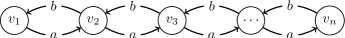
Figure 1. The digraph $G(n;a,b)$ with vertex set $\{v_{1},\ldots,v_{n}\}$, and with $a$ edges from $v_{i}$ to $v_{i+1}$ and $b$ edges from $v_{i+1}$ to $v_{i}$ ($i\in\{1,\ldots,n-1\}$).

Lemma 4.2.

Let $n,a,b$ be positive integers, and let $k:=\gcd(a,b)$. Then

$$\mathcal{B}(G(n;a,b),v_{1};y) =y^{(n-1)(a+b-d)}\left(\frac{1-y^{k}}{1-y}\right)^{n-1}.$$

Proof.

We start with the case when $\gcd(a,b)=1$. Note that, for any $i\in\{1,\ldots,n-1\}$, the number of reverse arborescences of $G(n;a,b)$ rooted at $v_{i}$ is equal to $b^{n-i}a^{i-1}$. Hence the period constant $\alpha$ of $G(n;a,b)$ is equal to

$$\alpha=\gcd_{1\leq i\leq n-1}b^{n-i}a^{i-1}=\gcd(a,b)^{n-1}=1.$$

By Lemma 3.5, this implies that $\textnormal{Rec}(G(n;a,b,),\stackrel{{\scriptstyle v_{1}}}{{\sim}})$ contains only one element.

Let $\widehat{\mathbf{c}}$ be the stable sink configuration of $G(n;a,b)$ with maximum level, i.e.

$$\widehat{\mathbf{c}}(v):=\begin{cases}\operatorname{\textnormal{outdeg}}(v)-1&\text{if }v\neq v_{1};\\ 0&\text{if }v=v_{1}.\end{cases}$$

Since $\textnormal{Rec}(G(n;a,b,),\stackrel{{\scriptstyle v_{1}}}{{\sim}})$ contains only one element, we conclude that $[\widehat{\mathbf{c}}]_{v_{1}}$ is the unique element in $\textnormal{Rec}(G(n;a,b,),\stackrel{{\scriptstyle v_{1}}}{{\sim}})$. Hence we have:

$$\begin{split}\mathcal{B}(G(n;a,b),v_{1};y)=&y^{\textnormal{lvl}([\widehat{\mathbf{c}}]_{v_{1}})+\operatorname{\textnormal{outdeg}}(v_{1})}\\ =&y^{{\textnormal{lvl}(\widehat{\mathbf{c}})}+\operatorname{\textnormal{outdeg}}(v_{1})}\quad\text{(by the maximality of }\widehat{\mathbf{c}})\\ =&y^{(n-1)(a+b-1)}.\end{split}$$ (4)

We now proceed with the case when $k=\gcd(a,b)$ is arbitrary. Note that

$$\mathcal{B}(G(n;a,b),v_{1};y) =\mathcal{B}({G(n;a/k,b/k)},v_{1};y^{k})\left(\frac{1-y^{k}}{1-y}\right)^{n-1}\quad\text{(by Proposition~{}\ref{l. computation})}$$

$$=y^{(n-1)(a+b-k)}\left(\frac{1-y^{k}}{1-y}\right)^{n-1}\quad\text{(by equation~{}\eqref{equation: Gnab 1})}.\qed$$

By a similar argument as in Lemma 4.2, for any $k\geq 1$ and any strongly connected digraph $G$ with the period constant equal to 1,

$$\mathcal{B}(G^{k},s;y)=y^{k(|E(G)|-|V|+1))}\left(\frac{1-y^{k}}{1-y}\right)^{|V|-1}.$$

5. Connections to the greedoid polynomial

In this section we relate the Biggs-Merino polynomial to another invariant of digraphs called the greedoid polynomial.

5.1. Greedoid polynomial and reverse G-parking functions

Let $G$ be a directed graph. A directed path $P$ of $G$ of length $k$ is a sequence $e_{1}\ldots e_{k}$ such that for $i\leq\{1,\ldots,k-1\}$ the target vertex of $e_{i}$ is the source vertex of $e_{i+1}$.

Definition 5.1 (Arborescences).

Let $G$ be a strongly connected digraph. An arborescence $T$ of $G$ rooted at $s\in V$ is a subgraph of $G$ that contains $|V|-1$ edges and such that for any $v\in V$ there exists a unique directed path from $s$ to $v$ in the subgraph. ∎

Fix a total order $<$ on the directed edges of $G$. For any two distinct edge-disjoint directed paths $P_{1}$ and $P_{2}$, we write $P_{1}<P_{2}$ if the smallest edge in $E(P_{1})\sqcup E(P_{2})$ (with respect to $<$) is contained in $P_{1}$.

Definition 5.2 (External activity).

Let $T$ be an arborescence of a strongly connected digraph $G$ rooted at $s\in V$. For any edge $e\in E(G)\setminus E(T)$, there are exactly two edge-disjoint directed paths $P_{1}$ and $P_{2}$ that share the same starting vertex and ending vertex. Let $P_{1}$ be the path that contains $e$. We say that $e$ is externally active with respect to $T$ if $P_{1}<P_{2}$. The external activity $\textnormal{ext}(T)$ of $T$ is the number of edges in $G$ that are externally active with respect to $T$. ∎

See Figure 2 for an illustration describing the process in Definition 5.2.

(a)	(b)	(c)

Figure 2. (a) An arborescence $T$. (b) An arborescence $T$ with an extra edge $e$. (c) The (undashed) path $P_{1}$ that contains $e$ and the (dashed) path $P_{2}$ that doesn’nt contain $e$.

Definition 5.3 (Greedoid polynomial).

Let $G$ be a strongly connected digraph, and let $s\in V$. The (single variable) greedoid polynomial is

$$T(G,s;y):=\sum_{T}y^{\textnormal{ext}(T)},$$

with the sum taken over all arborescences of $G$ rooted at $s$. ∎

This definition of the greedoid polynomial is due to Björner, Korte, and Lovász [BKL85]. Their definition encompasses a bigger for a more general family of combinatorial objects called greedoids, of which the polynomial in Definition 5.3 is a special case.

The polynomial $T(G,s;y)$ does not depend on the choice of total order $<$ on the edges [BKL85, Theorem 6.1]. If $G$ is a loopless undirected graph, then the greedoid polynomial $T(G,s;y)$ of $G$ (considered as a bidirected digraph) is equal to $y^{E(G)}\mathcal{T}(G;1,y)$, where $\mathcal{T}(G;x,y)$ is the Tutte polynomial of $G$ (considered as an undirected graph) [BKL85]. We remark that the extra factor $y^{E(G)}$ is due to undirected edges of $G$ being considered as two separate directed edges.

We refer the reader to [BZ92] for an introduction to greedoids and related topics, and [GM89, GT90, GM01] for a more detailed study of the greedoid polynomial.

Definition 5.4 (Reverse $G$-parking functions).

Let $G$ be a strongly connected digraph, and let $s\in V$. A reverse $G$-parking function with respect to $s$ is a function $f:V\setminus\{s\}\to\mathbb{N}_{0}$ such that, for any non-empty subset $A\subseteq V\setminus\{s\}$, there exists $v\in A$ for which $f(v)$ is strictly smaller than the number of edges from $V\setminus A$ to $v$. ∎

We use $\textnormal{Park}(G,s)$ to denote the set of reverse $G$-parking functions rooted at $s$.

$G$-parking functions were originally defined by Konheim and Weiss [KW66] for complete graphs, and were then extended to arbitrary digraphs by Postnikov and Shapiro [PS04]. Reverse $G$-parking functions are known under several different names, including reduced divisors [BS13], superstable configurations [HLM⁺08, AB10], and $\mathbf{\chi}$-superstable configurations [GK15].

We remark that the choice of working with reverse $G$-parking functions (instead of $G$-parking functions) is not due to a mere choice of convention, but is due to a duality property in the next lemma.

For any sink configuration $\widehat{\mathbf{c}}$ of $G$, its dual function $f:V\setminus\{s\}\to\mathbb{N}_{)}$ is given by

$$f(v):=\operatorname{\textnormal{outdeg}}(v)-1-\widehat{\mathbf{c}}(v)\quad(v\in V\setminus\{s\}).$$

Lemma 5.5 ([HLM⁺08, Theorem 4.4]).

Let $G$ be a connected Eulerian digraph, and let $s\in V$. Then a sink configuration of $G$ is sink recurrent if and only if its dual function is a reverse $G$-parking function. ∎

Remark.

We would like to warn the reader that Lemma 5.5 is false if $G$ is not an Eulerian digraph. For an arbitrary (strongly connected) digraph, the functions dual to recurrent sink configurations are called z-superstable configurations [AB10, GK15]. We refer the reader to [GK15, Section 4] (specifically, Example 4.17) for the subtle distinction between these two functions. ∎

Definition 5.6 (Level of a function).

The level of a function $f:V\setminus\{s\}\to\mathbb{N}_{0}$ is

$$\textnormal{lvl}(f):=|E|-|V|+1-\sum_{v\in V\setminus\{s\}}f(v).\qed$$

Note that the level of a function is equal to level of its dual sink configuration plus the outdegree of $s$.

5.2. Cori-Le Borgne bijection for directed graphs

In this subsection we give a bijection between reverse $G$-parking functions and arborescences of a directed graph $G$. This bijection is a directed graph version of Cori-Le Borgne bijection [CLB03, BS13] for undirected graphs. For the description of this bijection, see Algorithm 1.

Input:

$G$-parking function $f$ with respect to $s$,

Total order on the edges of $G$.

Output:

Arborescence $T_{f}$ of $G$ rooted at $s$.

1

2Initialization:

3$\textnormal{BV}:=\{s\}$ (burnt vertices),

4$\textnormal{BE}:=\emptyset$ (burnt edges),

5$T:=\emptyset$ (directed tree).

6while $\textnormal{BV}\neq V(G)$  do

7       $e:=\max\{(v,w)\in E(G)\,|\,(v,w)\not\in\textnormal{BE},\,v\in\textnormal{BV},w\not\in\textnormal{BV}\}$,

8       $w:=$ the target vertex of $e$,

9       if $f(w)==$ the number of edges in BE with $w$ as the target vertex  then

10             $\textnormal{BV}\leftarrow\textnormal{BV}\cup\{w\}$,

11             $T\leftarrow T\cup\{e\}$,

12       end if

13      $\textnormal{BE}\leftarrow\textnormal{BE}\cup\{e\}$

14 end while

Output $T_{f}:=T$.

Algorithm 1 Cori-Le Borge bijection from $G$-parking functions to arborescences of $G$.

Theorem 1.2.

Let $G$ be a strongly connected digraph, and let $s\in V$. Then Algorithm 1 is a bijection that sends reverse $G$-parking functions with respect to $s$ to arborescences of $G$ rooted at $s$. Furthermore, the external activity of the output arborescence is the level of the input reverse $G$-parking function.

Remark.

There are several bijections in the existing literature between $G$-parking functions and spanning trees of undirected graphs (for example [Big99, KY08, Bac12, ABKS14, PYY17]). For directed graphs, there is a bijection between reverse $G$-parking functions and arborescences of $G$ by Chebikin and Pylyavskyy [CP05]. Note that this bijection is different from the bijection in Algorithm 1 as the former does not preserve the notion of activities (see [CP05, Section 5]). ∎

The following theorem is a direct consequence of Theorem 1.2 and Lemma 5.5.

Theorem 1.3 (Merino’s Theorem for Eulerian digraphs).

Let $G$ be a connected Eulerian digraph. Then for any $s\in V$,

$$T(G,s;y)=\sum_{\widehat{\mathbf{c}}\in\textnormal{Rec}(G,s)}y^{\textnormal{lvl}(\widehat{\mathbf{c}})+\operatorname{\textnormal{outdeg}}(s)}.\qed$$

If the graph in Theorem 1.3 is bidirected, then we recover the original theorem of Merino López [ML97].

Remark.

We would like to warn the reader that there are non-Eulerian digraphs for which Theorem 1.3 is false. This is because $T(G,s;1)$ is the number of arborescences of $G$, while $|\textnormal{Rec}(G,s)|$ is the number of reverse arborescences of $G$ (by Lemma 2.13(ii)). Those two numbers are in general not equal for non-Eulerian digraphs. ∎

The following corollary is a consequence of Theorem 1.3.

Corollary 5.7.

Let $G$ be a connected Eulerian digraph. Then for any $s\in V$,

$$T(G,s;y)=\mathcal{B}(G,s;y).$$

Proof.

Since $G$ is a connected Eulerian digraph, the primitive period vector $\mathbf{r}$ of $G$ is equal to $(1,\ldots,1)$. By the markov chain tree theorem [AT89], this implies that the period constant $\alpha$ is equal to the number of reverse arborescences rooted at $s$. By Proposition 3.5 and Lemma 2.13(ii), this implies that there are as many recurrent sink classes as recurrent sink configurations. Hence we conclude that each recurrent sink class of $G$ contains a unique recurrent sink configuration. Together with Theorem 1.3, this implies that

$$T(G,s;y)=\sum_{\widehat{\mathbf{c}}\in\textnormal{Rec}(G,s)}y^{\textnormal{lvl}(\widehat{\mathbf{c}})+\operatorname{\textnormal{outdeg}}(s)}=\sum_{[\widehat{\mathbf{c}}]\in\textnormal{Rec}(G,\stackrel{{\scriptstyle\text{s}}}{{\sim}})}y^{\textnormal{lvl}([\widehat{\mathbf{c}}])}=\mathcal{B}(G,s;y).\qed$$

This relates the Biggs-Merino polynomial to the greedoid polynomial, as promised in the beginning of this section.

Corollary 5.7 gives two interesting consequences for a connected Eulerian digraph $G$. The first consequence is that the greedoid polynomial $T(G,s;y)$ does not depend on the choice of $s$ (by Theorem 3.7). The second consequence is that $\mathcal{B}(G,s;2)$ counts the number of subgraphs of $G$ such that, for any $v\in V$, there exists a directed path from $s$ to $v$ in the subgraph (since $T(G,s;2)$ counts the same thing by [GM89, Lemma 2.1]).

Remark.

We would like to warn the reader that Corollary 5.7 is false when $G$ is a non-Eulerian digraph. This is because the number of reverse arborescences of $G$ depends on the choice of $s$ if $G$ is non-Eulerian, while $\mathcal{B}(G,s;y)$ does not depend on the choice of $s$ (by Theorem 3.7). ∎

The rest of this section is focused on the proof of Theorem 1.2.

For any $G$-parking function $f$, denote by $T_{f}$ the output of Algorithm 1, denote by $\textnormal{BV}(f)$ the set of vertices that are burnt in Algorithm 1, and by $\textnormal{BE}(f)$ the set of edges that are burnt in Algorithm 1.

Lemma 5.8.

Let $G$ be a strongly connected digraph, let $s\in V$, and let $f$ be a $G$-parking function with respect to $s$. Then:

1. $\textnormal{BV}(f)=V(G)$;

2. $f(v)=|\{e\in\textnormal{BE}(f)\mid\textnormal{trgt}(e)=v\}|$ for all $v\in V$; and

3. $T_{f}$ is an arborescence of $G$ rooted at $s$.

Proof.

1. Suppose to the contrary that Algorithm 1 terminates when $\textnormal{BV}(f)\subsetneq V(G)$. Line 1-1 of the algorithm imply that all edges with source vertex in $\textnormal{BV}(f)$ and target vertex in $V(G)\setminus\textnormal{BV}(f)$ are burnt. Write $A:=V(G)\setminus\textnormal{BV}(f)$. Line 1 of the algorithm then implies that for all $v\in A$, the function $f(v)$ is greater than or equal to the number of edges $V(G)\setminus A$ to $v$. This contradicts the assumption that $f$ is a $G$-parking function, as desired.

2. Since $\textnormal{BV}(f)=V(G)$ by Lemma 5.8(i), Line 1 of Algorithm 1 implies that $f(v)$ is equal to the number of burnt edges with target vertex $v$ for all $v\in V$, as desired.

3. It follows from Line 1-1 of Algorithm 1 that $T_{f}$ is a directed tree with $|\textnormal{BV}(f)|-1$ edges and with $s$ as the unique source vertex. Since $\textnormal{BV}(f)=V(G)$ by Lemma 5.8(i), it then follows that $T_{f}$ is an arborescence of $G$ rooted at $s$. ∎

Lemma 5.9.

Let $G$ be a strongly connected digraph, let $s\in V$, and let $f$ be a $G$-parking function with respect to $v$. Then an edge $e\in E(G)\setminus E(T_{f})$ is externally active with respect to $T_{f}$ if and only if $e$ is not contained in $\textnormal{BE}(f)$.

Proof.

Let $P_{1}$ and $P_{2}$ be two edge-disjoint directed paths as in Definition 5.2. Note that $e$ is contained in $P_{1}$ by definition. Let $e^{\prime}$ be the minimum edge in $E(P_{1})\sqcup E(P_{2})$. We need to show that $e^{\prime}$ is contained in $P_{2}$ if and only if $e$ is contained in $\textnormal{BE}(f)$.

Suppose that $e^{\prime}$ is contained in $P_{2}$. By the minimality of $e^{\prime}$, it then follows that the source vertex of $e$ is burnt before $e^{\prime}$ in the while loop of Algorithm 1. Again by the minimality of $e^{\prime}$, it then follows that $e$ is evaluated before $e^{\prime}$ in the while loop of the algorithm. Since $e$ is not contained in $T_{f}$, it then follows that $e$ is burnt when it is evaluated. This proves one direction of the claim.

Suppose that $e^{\prime}$ is contained in $P_{1}$. By the minimality of $e^{\prime}$, it then follows that all edges in $P_{2}$ are evaluated before $e^{\prime}$ in the while loop of Algorithm 1. This implies that all vertices in $P_{2}$ is burnt before $e^{\prime}$ is evaluated by the while loop. Since $P_{1}$ and $P_{2}$ share the same target vertex and $e$ is the last edge in $P_{1}$, it then follows that $e$ is either not evaluated or evaluated after its target vertex is burnt in the while loop. In either cases $e$ is not burnt in the while loop. This proves the other direction of the claim. ∎

We now give an algorithm that will provide the inverse map to Algorithm 1 (note that at this point we have not yet shown that Algorithm 1 is a bijection). See Algorithm 2 for the description of the algorithm.

Input:

Arborescence $T$ of $G$ rooted at $s$,

Total order on the edges of $G$.

Output:

$G$-parking function $f_{T}$ with respect to $s$.

1

2Initialization:

3$\textnormal{BV}:=\{s\}$ (burnt vertices),

4$\textnormal{BE}:=\emptyset$ (burnt edges).

5while $\textnormal{BV}\neq V(G)$  do

6       $e:=\max\{(v,w)\in E(G)\,|\,(v,w)\not\in\textnormal{BE},\,v\in\textnormal{BV},w\not\in\textnormal{BV}\}$,

7       $w:=$ the target vertex of $e$,

8       if $e\in E(T)$  then

9             $\textnormal{BV}\leftarrow\textnormal{BV}\cup\{w\}$,

10       end if

11      $\textnormal{BE}\leftarrow\textnormal{BE}\cup\{e\}$

12 end while

Output $f_{T}$, with $f_{T}(v):=$ the number of edges in BE with $v$ as target vertex (for $v\in V\setminus\{s\}$).

Algorithm 2 Cori-Le Borge bijection from arborescences of $G$ to $G$-parking functions.

For any arborescence $T$ of $G$, denote by $f_{T}$ the output of Algorithm 2, denote by $\textnormal{BV}(T)$ the set of vertices that are burnt in Algorithm 2, and by $\textnormal{BE}(T)$ the set of edges that are burnt in Algorithm 2.

Lemma 5.10.

Let $G$ be a strongly connected digraph, let $s\in V$, and let $T$ be an arborescence of $G$ rooted at $s$. Then:

1. $f_{T}$ is a $G$-parking function with respect to $s$; and

2. For any $G$-parking function $f$ with respect to $s$, we have $f_{T_{f}}=f$.

Proof.

1. Let $A$ be an arbitrary non-empty subset of $V\setminus\{s\}$. Since $T$ is an arborescence of $G$, it follows that Algorithm 2 terminates only when all vertices are burnt. Let $v$ be the first vertex in $A$ that is burnt by Algorithm 2. By the minimality assumption on $v$, it then follows that the source vertex of every edge in $\{e\in\textnormal{BE}(T)\mid\textnormal{trgt}(e)=v\}$ is contained in $V\setminus A$. Also note that any edge in $T$ is not burnt in Algorithm 2. Hence:

   $$f_{T}(v)= |\{e\in\textnormal{BE}(T)\mid\textnormal{trgt}(e)=v\}|$$

   $$\leq |\{e\in E(G)\mid\textnormal{src}(e)\in V\setminus A,\textnormal{trgt}(e)=v,\text{ and }e\notin E(T)\}|$$

   $$= \,\text{the number of edges from $V\setminus A$ to $v$}\ -1.$$

   Since the choice of $A$ is arbitrary, this shows that $f_{T}$ is a $G$-parking function.

2. It follows from the description of Algorithm 1 and Algorithm 2 that $\textnormal{BE}(f)=\textnormal{BE}(T_{f})$. It then follows from Lemma 5.8(ii) that $f=f_{T_{f}}$. ∎

Proof of Theorem 1.2.

Note that Algorithm 1 maps $G$-parking functions to arborescences of $G$ (by Lemma 5.8(iii)). Also note that Algorithm 2 maps arborescences of $G$ to $G$-parking functions (by Lemma 5.10(i)). Finally, note that applying Algorithm 2 after Algorithm 1 sends a $G$-parking function back to itself. These three statements imply that Algorithm 1 is a bijection from $G$-parking functions to arborescences of $G$, and Algorithm 2 is its inverse.

It follows from Lemma 5.8(ii) and Lemma 5.9 that $\textnormal{ext}(T_{f})=\textnormal{lvl}(f)$ for any $G$-parking function $f$. The proof is complete. ∎

6. Concluding remarks

In this section we present a few unanswered questions that might warrant further research.

As remarked in Section 5, there are non-Eulerian digraphs for which the conclusion of Theorem 1.3 and Corollary 5.7 are false. A further research can be done on extending these two theorems to general digraphs, and here we list two questions of that flavor.

Question 6.1.

Let $G$ be a non-Eulerian strongly connected digraph.

1. Does there exist a greedoid for which its greedoid polynomial satisfies the conclusion of Theorem 1.3 or Corollary 5.7?

2. Does there exist an expression for the polynomial in the right hand side of Theorem 1.3 or Corollary 5.7 that is not related to the sandpile model?

Note that Question 6.1(i) is a special case of Question 6.1(ii).

One consequence of Merino’s Theorem for undirected graphs is that it implies Stanley’s pure $O$-sequence conjecture [Sta96] for cographic matroids. It is therefore natural to ask for a relationship between our works and $O$-sequences.

Let $X$ be a finite, nonempty set of (monic) monomials in the indeterminates $x_{1},\ldots,x_{k}$. We call $X$ a (monomial) order ideal if, for any monomial $m_{1}\in X$ and any monomial $m_{2}$, we have $m_{2}$ divides $m_{1}$ only if $m_{2}\in X$. An order ideal $X$ is pure if all the maximal monomials in $X$ (i.e. polynomials that are not divisible by any other elements in $X$) have the same degree.

Let $h_{i}$ $(i\geq 0)$ denote the number of monomials in $X$ with degree $i$. The $h$-vector of $X$ is the vector ($h_{0},\ldots,h_{n}$), where $n$ is the maximum degree of monomials in $X$. An $O$-sequence is the $h$-vector of an order ideal, and a pure $O$-sequence is the $h$-vector of a pure order ideal.

It follows from Theorem 1.2 that, for any strongly connected digraph $G$, the nonzero coefficients of its greedoid polynomial, ordered from the highest degree to the lowest degree, is an $O$-sequence. A further research can be done on extending this observation to other classes of greedoids.

Question 6.2.

Do the nonzero coefficients of the greedoid polynomial of a greedoid form an $O$-sequence? If not, what is the class of greedoids for which this property holds?

We remark that there are Eulerian digraphs for which the corresponding $O$-sequence is not pure, for example [PP15, Figure 10].

Another possible research direction is on the method of computing the Biggs-Merino polynomial efficiently. There is a variant of the deletion-contraction recursion [BKL85] for the greedoid polynomial and a Möbius inversion formula [PP16] for the Biggs-Merino polynomial of an Eulerian digraph. However, we are not aware of any formulas of the same type for the Biggs-Merino polynomial of non-Eulerian digraphs.

Question 6.3.

Does there exist any kind of deletion-contraction recurrence for the Biggs-Merino polynomial of non-Eulerian digraphs?

References

• [AB10] Arash Asadi and Spencer Backman. Chip-firing and Riemann-Roch theory for directed graphs, December 2010.
• [ABKS14] Yang An, Matthew Baker, Greg Kuperberg, and Farbod Shokrieh. Canonical representatives for divisor classes on tropical curves and the matrix-tree theorem. Forum Math. Sigma, 2:e24, 25, 2014.
• [AT89] V. Anantharam and P. Tsoucas. A proof of the Markov chain tree theorem. Statist. Probab. Lett., 8(2):189–192, 1989.
• [Bac12] Spencer Backman. A bijection between the recurrent configurations of a hereditary chip-firing model and spanning trees, July 2012.
• [Big97a] Norman Biggs. Combinatorial Theory Seminar, Mathematical Institute, Oxford University, February 1997.
• [Big97b] Norman Biggs. Algebraic potential theory on graphs. Bull. London Math. Soc., 29(6):641–682, 1997.
• [Big99] Norman Biggs. The Tutte polynomial as a growth function. J. Algebraic Combin., 10(2):115–133, 1999.
• [BKL85] Anders Björner, Bernhard Korte, and László Lovász. Homotopy properties of greedoids. Adv. in Appl. Math., 6(4):447–494, 1985.
• [BL92] Anders Björner and László Lovász. Chip-firing games on directed graphs. J. Algebraic Combin., 1(4):305–328, 1992.
• [BL16a] Benjamin Bond and Lionel Levine. Abelian networks I. Foundations and examples. SIAM J. Discrete Math., 30(2):856–874, 2016.
• [BL16b] Benjamin Bond and Lionel Levine. Abelian networks II. Halting on all inputs. Selecta Math. (N.S.), 22(1):319–340, 2016.
• [BL16c] Benjamin Bond and Lionel Levine. Abelian networks III. The critical group. J. Algebraic Combin., 43(3):635–663, 2016.
• [BLS91] Anders Björner, László Lovász, and Peter W. Shor. Chip-firing games on graphs. European J. Combin., 12(4):283–291, 1991.
• [BN07] Matthew Baker and Serguei Norine. Riemann-Roch and Abel-Jacobi theory on a finite graph. Adv. Math., 215(2):766–788, 2007.
• [BS13] Matthew Baker and Farbod Shokrieh. Chip-firing games, potential theory on graphs, and spanning trees. J. Combin. Theory Ser. A, 120(1):164–182, 2013.
• [BTW88] Per Bak, Chao Tang, and Kurt Wiesenfeld. Self-organized criticality. Phys. Rev. A (3), 38(1):364–374, 1988.
• [BZ92] Anders Björner and Günter M. Ziegler. Introduction to greedoids. In Matroid Applications, pages 284–357. Cambridge University Press, 1992. Cambridge Books Online.
• [CLB03] Robert Cori and Yvan Le Borgne. The sand-pile model and Tutte polynomials. Adv. in Appl. Math., 30(1-2):44–52, 2003.
• [CP05] Denis Chebikin and Pavlo Pylyavskyy. A family of bijections between $G$-parking functions and spanning trees. J. Combin. Theory Ser. A, 110(1):31–41, 2005.
• [Dha90] Deepak Dhar. Self-organized critical state of sandpile automaton models. Phys. Rev. Lett., 64(14):1613–1616, 1990.
• [GK15] Johnny Guzmán and Caroline Klivans. Chip-firing and energy minimization on M-matrices. Journal of Combinatorial Theory, Series A, 132(0):14 – 31, 2015.
• [GM89] Gary Gordon and Elizabeth McMahon. A greedoid polynomial which distinguishes rooted arborescences. Proc. Amer. Math. Soc., 107(2):287–298, 1989.
• [GM01] Gary Gordon and Elizabeth McMahon. A characteristic polynomial for rooted graphs and rooted digraphs. Discrete Math., 232(1-3):19–33, 2001.
• [GT90] Gary Gordon and Lorenzo Traldi. Generalized activities and the Tutte polynomial. Discrete Math., 85(2):167–176, 1990.
• [HLM+08] Alexander E. Holroyd, Lionel Levine, Karola Mészáros, Yuval Peres, James Propp, and David B. Wilson. Chip-firing and rotor-routing on directed graphs. In In and out of equilibrium. 2, volume 60 of Progr. Probab., pages 331–364. Birkhäuser, Basel, 2008.
• [KW66] Alan G. Konheim and Benjamin Weiss. An occupancy discipline and applications. SIAM Journal on Applied Mathematics, 14(6):pp. 1266–1274, 1966.
• [KY08] Dimitrije Kostić and Catherine H. Yan. Multiparking functions, graph searching, and the Tutte polynomial. Adv. in Appl. Math., 40(1):73–97, 2008.
• [Lor89] Dino J. Lorenzini. Arithmetical graphs. Math. Ann., 285(3):481–501, 1989.
• [ML97] Criel Merino López. Chip firing and the Tutte polynomial. Ann. Comb., 1(3):253–259, 1997.
• [PP15] Kévin Perrot and Trung Van Pham. Feedback arc set problem and NP-hardness of minimum recurrent configuration problem of chip-firing game on directed graphs. Ann. Comb., 19(2):373–396, 2015.
• [PP16] Kévin Perrot and Trung Van Pham. Chip-firing game and a partial Tutte polynomial for Eulerian digraphs. Electron. J. Combin., 23(1):Paper 1.57, 34, 2016.
• [PPW13] David Perkinson, Jacob Perlman, and John Wilmes. Primer for the algebraic geometry of sandpiles. In Tropical and non-Archimedean geometry, volume 605 of Contemp. Math., pages 211–256. Amer. Math. Soc., Providence, RI, 2013.
• [PS04] Alexander Postnikov and Boris Shapiro. Trees, parking functions, syzygies, and deformations of monomial ideals. Trans. Amer. Math. Soc., 356(8):3109–3142 (electronic), 2004.
• [PYY17] David Perkinson, Qiaoyu Yang, and Kuai Yu. $G$-parking functions and tree inversions. Combinatorica, 37(2):269–282, 2017.
• [Spe93] Eugene R. Speer. Asymmetric abelian sandpile models. J. Statist. Phys., 71(1-2):61–74, 1993.
• [Sta96] Richard P. Stanley. Combinatorics and commutative algebra, volume 41 of Progress in Mathematics. Birkhäuser Boston, Inc., Boston, MA, second edition, 1996.
• [Tar88] Gábor Tardos. Polynomial bound for a chip firing game on graphs. SIAM J. Discrete Math., 1(3):397–398, 1988.