Spiral Toolpaths for High-Speed Machining of 2D Pockets with or without Islands

Abstract

We describe new methods for the construction of spiral toolpaths for high-speed machining. In the simplest case, our method takes a polygon as input and a number $\delta>0$ and returns a spiral starting at a central point in the polygon, going around towards the boundary while morphing to the shape of the polygon. The spiral consists of linear segments and circular arcs, it is $G^{1}$ continuous, it has no self-intersections, and the distance from each point on the spiral to each of the neighboring revolutions is at most $\delta$. Our method has the advantage over previously described methods that it is easily adjustable to the case where there is an island in the polygon to be avoided by the spiral. In that case, the spiral starts at the island and morphs the island to the outer boundary of the polygon. It is shown how to apply that method to make significantly shorter spirals in polygons with no islands than what is obtained by conventional spiral toolpaths. Finally, we show how to make a spiral in a polygon with multiple islands by connecting the islands into one island.

1 Introduction

A fundamental problem often arising in the CAM industry is to find a suitable toolpath for milling a pocket that is defined by a shape in the plane. A CNC milling machine is programmed to follow the toolpath and thus cutting a cavity with the shape of the given pocket in a solid piece of material. The cutter of the machine can be regarded as a circular disc with radius $r$, and the task is to find a toolpath in the plane such that the swept volume of the disc, when the disc center is moved along the path, covers the entire pocket. We assume for simplicity that the toolpath is allowed to be anywhere in the pocket.

Some work has been made on spiral toolpaths that morphs a point within the pocket to the boundary of the pocket [2, 3, 10, 1, 11, 12]. The method described by Held and Spielberger [10] yields a toolpath that (i) starts at a user-specified point within the pocket, (ii) ends when the boundary is reached, (iii) makes the cutter remove all material in the pocket, (iv) has no self-intersections, (v) is $G^{1}$ continuous, (vi) makes the width of material cut away at most $\delta$ at any time, where $\delta$ is a user-defined constant called the stepover. We must have $\delta<r$, since otherwise some material might not be cut away. See figure 3 for an example of such a spiral toolpath. It is the result of an algorithm described in the present paper, but has similar appearance as the spirals described by Held and Spielberger [10].

Most traditional toolpath patterns have many places where the cutter does not cut away any new material, for instance in retracts where it is lifted and moved in the air to another place for further machining, or self-intersections of the toolpath, where the tool does not cut away anything new when it visits a place for the second time. That may increase machining time and lead to visible marks on the final product. Spiral toolpaths have the advantage that the cutter is cutting during all of the machining and that, at the same time, the user can control the stepover. Spiral toolpaths are particularly useful when doing high-speed machining, where the rotational speed of the cutter and the speed with which it is moved along the toolpath is higher than in conventional milling. We refer to Held and Spielberger [10] for a more detailed discussion of the benefits of spiral toolpaths compared to various other toolpath patterns and more information on CNC milling in general.

Bieterman and Sandstrom [2] and Huertas-Talón et al. [12] give methods for computing spiral toolpaths by solving elliptic partial differential equation boundary value problems defined on the pocket. However, the methods only work for star-shaped pockets [10].

We describe an alternative construction of spirals that also satisfy the previously mentioned properties of the construction of Held and Spielberger [10]. They define a wave that starts at a point in the Voronoi diagram of the pocket at time $0$. When the time increases, the wave moves towards the boundary of the pocket in every direction so that at time $1$, it reaches the boundary everywhere. The shape of the wave at a certain time represents the area machined at that time. Roughly speaking, the spiral is obtained by traveling around the wave while the time increases from $0$ to $1$. Our method is similar up to this point, but the way we define the wave is different. The wave defined in [10] is the union of growing disks placed on the Voronoi diagram of the pocket. In our model, the wave is at any time a polygon with its corners on the Voronoi diagram of the pocket. Using that model, we define a spiral consisting of line segments which is at last rounded by circular arcs to get a $G^{1}$ continuous curve.

In practice, it is very common that there is one or more islands in the pocket that should be avoided by the cutter, for instance if there are areas of material that should not be machined to the same depth. It is only described by Held and Spielberger [10] how to handle simply-connected pockets, i.e., there must be no islands. In their following paper [11], it is described how one can handle a pocket with an island by connecting it to the boundary with a “bridge”, effectively getting a pocket without islands. Thus, the resulting spiral morphs a point to a shape consisting of the island, the bridge, and the pocket boundary. A big advantage of our method is that it has a natural extension to pockets with one island in the sense that the spiral morphs the shape of the island to the pocket boundary. We exploit the fact that the Voronoi diagram of a pocket with an island consists of exactly one cycle and trees rooted at that cycle to extend our wave model to work in this case. This is our biggest new contribution. We shall demonstrate natural applications of this method to make significantly shorter spirals for pockets with no holes than one could obtain with previously described methods. We also show how to handle pockets with multiple holes.

The paper is based on the author’s experiences while developing the morphed spiral strategy for the Autodesk™ CAM products (HSMWorks, Inventor HSM^®, and Fusion 360^®). The morphed spiral seems to be quite popular among the users. Due to the abundant number of real-world parts that have been available during the development, we guarantee that it is possible to make an efficient industrial-strength implementation of the algorithms described here.

We use Held’s VRONI library for the computation of Voronoi diagrams [8]. All figures in the paper are automatically generated using our implementation of the algorithms.

The rest of the paper is structured as follows: In section 2, we describe our basic method for making a spiral that morphs a point to the boundary in a simply-connected pocket. Section 3 describes how the method is adapted to a pocket with one island. Using that method, we describe in section 4 an alternative spiral in simply-connected pockets which will be superior to the one from section 2 in many cases. In section 5, we show how to construct at spiral around arbitrarily many islands by first connecting the islands into one island. Finally, we conclude the paper in section 6 by suggesting some future paths of development of spiral toolpaths.

1.1 Notation and other general conventions

We use zero-based numbering of arrays. For a point $p=(x,y)$, the point $\widehat{p}=(-y,x)$ is the counterclockwise rotation of $p$. Given two distinct points $p$ and $q$, $pq$ is the segment between $p$ and $q$ and $\overrightarrow{pq}$ is the half-line that starts at $p$ and contains $q$. Given a set of points $S$ in the plane, $\partial S$ denotes the boundary of $S$. In algorithms, we use semicolon to separate different statements written on the same line.

2 Computing a spiral in a pocket without islands

In this section we describe a method to compute a spiral in a given simply-connected 2D pocket $\mathcal{P}$, see figure 3. In practice, the boundary of a pocket is often described by line segments and more advanced pieces of curves, such as like circular arcs, elliptic arcs, and splines. However, it is always possible to use a sufficiently accurate linearization of the input, so we assume for simplicity that $\mathcal{P}$ is a polygon.

Our algorithm first constructs a polyline spiral, see figure 3. The polyline spiral must respect the stepover $\delta$, i.e., the distance from every point to the neighboring revolutions and the distance from the outermost revolution to $\partial\mathcal{P}$ is at most $\delta$. In section 2.9 we devise a method for rounding the polyline spiral to get a $G^{1}$ continuous spiral consisting of line segments and circular arcs.

The corners of the polyline spiral are points on the edges of the Voronoi diagram of $\mathcal{P}$, and there is a corner at each intersection point between the spiral and the Voronoi diagram. We only consider the part of the Voronoi diagram inside $\mathcal{P}$. We have found that we get better results in practice by modifying the Voronoi diagram slightly. We describe these modifications in sections 2.7 and 2.8 to avoid too many technical details here. See figures 1–1 for a concrete example of the modifications we make on the Voronoi diagram. Let $\mathcal{VD}=\mathcal{VD}(\mathcal{P})$ be the modified Voronoi diagram of the pocket $\mathcal{P}$. Like the Voronoi diagram of $\mathcal{P}$, the modified diagram $\mathcal{VD}$ has the following properties which are necessary and sufficient for the computation of the spiral:

• $\mathcal{VD}$ is a plane tree contained in $\mathcal{P}$,

• each leaf of $\mathcal{VD}$ is on the boundary $\partial\mathcal{P}$ of $\mathcal{P}$,

• there is at least one leaf of $\mathcal{VD}$ on each corner of $\mathcal{P}$,

• all the faces into which $\mathcal{VD}$ divides $\mathcal{P}$ are convex.

Figure 1: 1 The Voronoi diagram. 1 The Voronoi diagram enriched with equidistantly placed segments perpendicular to long edges. 1 The final diagram $\mathcal{VD}$ where double edges going to concave corners of $\mathcal{P}$ are replaced by their angle bisector.

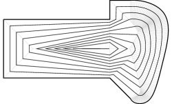
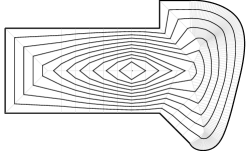
Figure 2: The wavefronts in the same polygon $\mathcal{P}$ for the same stepover $\delta$ but using two different diagrams to define the wavefronts. 2 The wavefronts obtained using the Voronoi diagram. The Voronoi diagram is in gray. 2 The wavefronts obtained using $\mathcal{VD}$. $\mathcal{VD}$ is in gray.

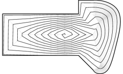
Figure 3: 3 The polyline spiral and $\mathcal{VD}$ in gray. 3 The final rounded spiral.

2.1 The wave model

We imagine that a wave starts at time $t=0$ at the point $p_{0}$ inside $\mathcal{P}$. The wave moves out in every direction such that at time $t=1$, it has exactly the same shape as $\partial\mathcal{P}$. The shape of the wave at a specific time is called a wavefront. The wave is growing in the sense that if $0\leq t_{1}\leq t_{2}\leq 1$, the wavefront at time $t_{1}$ is contained in the wavefront at time $t_{2}$. We choose $p_{0}$ as a point in the diagram $\mathcal{VD}$ and consider $\mathcal{VD}$ as a tree rooted at $p_{0}$. We define the time at which the wave hits each node and the speed with which it travels on each edge in $\mathcal{VD}$. The speed of the wave is always constant or decreasing. Thus, we create a continuous map $\theta:\mathcal{VD}\mapsto[0,1]$ that assigns a time value between 0 and 1 to each point on $\mathcal{VD}$. If $p$ is a point moving along a path on $\mathcal{VD}$ from $p_{0}$ to any leaf, the value $\theta(p)$ increases monotonically from 0 to 1. For each time $t\in[0,1]$, the wavefront is a polygon inside $\mathcal{P}$ and the vertices of the wavefront are all the points $p$ on $\mathcal{VD}$ such that $\theta(p)=t$. Note that there is exactly one such point on each path from $p_{0}$ to a leaf of $\mathcal{VD}$ for a given $t\in[0,1]$.

We define a time step $\Delta=1/r$ for some integer $r$ and compute the wavefront at the times $t\in\{0,\Delta,2\Delta,\ldots,r\Delta\}$, where $r\Delta=1$, see figure 2. By wavefront $i$, we mean the wavefront at time $i\Delta$. We choose $r$ such that the distance from each point on wavefront $i$ to each of the wavefronts $i-1$ and $i+1$ is at most $\delta$ when $i>0$ and $i<r$, respectively. In other words, the Hausdorff distance between two neighboring wavefronts is at most $\delta$. Recall that the Hausdorff distance between two sets $A$ and $B$ is $\max\{d(A,B),d(B,A)\}$, where $d(A,B)=\max_{a\in A}\min_{b\in B}\lVert a-b\rVert$. For each $i=1,\ldots,r$, we compute a revolution of the polyline spiral by interpolating between the wavefronts $i-1$ and $i$. We describe in sections 2.5 and 2.6 how to make the wavefronts and the interpolation such that the stepover is respected between neighboring revolutions.

2.2 Choosing the starting point $p_{0}$ and the number of revolutions of the spiral

In order to get a spiral with small length, we try to minimize the number of revolutions. Consider the longest path from $p_{0}$ to a leaf in $\mathcal{VD}$. The length of a path is the sum of edge lengths on the path. If $h$ is the length of the longest path, then $\lceil h/\delta\rceil+1$ wavefronts are necessary and sufficient for the stepover to be respected between all neighboring wavefronts. Therefore, we choose $p_{0}$ as the point in $\mathcal{VD}$ that minimizes the longest distance to a leaf in $\mathcal{VD}$. That is a unique point traditionally known as the center of $\mathcal{VD}$. Handler [7] gives a simple algorithm to compute $p_{0}$ linear time in the size of $\mathcal{VD}$. The center will most likely not be a node in $\mathcal{VD}$, but an interior point on some edge. In that case, we split the edge into two edges by introducing a node at $p_{0}$.

2.3 Our representation of $\mathcal{VD}$

We consider $\mathcal{VD}$ as a directed, rooted tree with the node Root at $p_{0}$ being the root. We let $\texttt{Pt}[n]$ be the position of the node $n$. Let $\mathcal{VD}[n]$ be the subtree rooted at node $n$. We store a pointer $\texttt{ParentE}[n]$ to the edge having end node $n\neq\texttt{Root}$. We say that edge $\texttt{ParentE}[n]$ is the parent edge of node $n$ and any edge having start node $n$. We also store an array $\texttt{ChildEs}[n]$ of the edges going out of $n$ sorted in counterclockwise order with the edge following $\texttt{ParentE}[n]$ being the first. For Root, the choice of the first child edge does not matter. For each edge $e$, we store pointers $\texttt{Start}[e]$ and $\texttt{End}[e]$ to the start and end nodes of $e$. We also store an index $i=\texttt{IndexInStart}[e]$ such that $\texttt{ChildEs}[\texttt{Start}[e]][i]=e$. If $e$ is an edge, we say that $\texttt{Start}[e]$ and $\texttt{End}[e]$ are incident to $e$ and that $e$ is incident to $\texttt{Start}[e]$ and $\texttt{End}[e]$. For an edge $e_{1}$ and node $n$ incident to $e_{1}$, we let $\texttt{NextCCW}(e_{1},n)=e_{2}$, where $e_{2}$ is the edge after $e_{1}$ among the edges incident to $n$ in counterclockwise order. The function NextCCW can be implemented so that it runs in constant time using the values defined here.

Using NextCCW, we can traverse all of $\mathcal{VD}$ in counterclockwise direction in linear time. We start setting $(n,e)=(\texttt{Root},\texttt{ChildEs}[\texttt{Root}][0])$. In each iteration, we let $n$ be the other node incident to $e$ and then set $e=\texttt{NextCCW}(e,n)$. We stop when we have traversed every edge, i.e., when $(e,n)=(\texttt{Root},\texttt{ChildEs}[\texttt{Root}][0])$ at the end of an iteration. Note that each edge $e$ is visited twice, once going down the tree $\mathcal{VD}[\texttt{Start}[e]]$ and once going up.

2.4 Defining the movement of the wave

Let $0pt[n]$ for each node $n$ be the maximal distance from $n$ to a leaf in $\mathcal{VD}[n]$. All the $0pt$ values can be computed in linear time by traversing $\mathcal{VD}$ once. For each node $n$, we define the time $\texttt{TmNd}[n]$ where the wave reaches $n$. We set $\texttt{TmNd}[\texttt{Root}]=0$. We also define the speed $\texttt{VeNd}[n]$ that the wave has when it reaches $n$. We set $\texttt{VeNd}[\texttt{Root}]=0pt[\texttt{Root}]$. The wave starts at the root at time $t=0$ and travels with constant speed $\texttt{VeNd}[\texttt{Root}]$ on the paths to the farthest leafs in $\mathcal{VD}$. (Due to our choice of the starting point $p_{0}$, there will always be at least two paths from $p_{0}$ to a leaf with maximum length.) Hence, it reaches those leafs at time $t=1$. On all the shorter paths, we make the wave slow down so that it reaches every leaf at time $t=1$. In A, we describe in detail a possible way of defining the speed and time of the wave on each point in $\mathcal{VD}$.

When the movement of the wave is defined, we may define $\texttt{GetPt}(e,t)$ as the point on edge $e$ with $\theta(\texttt{GetPt}(e,t))=t$, where $\texttt{TmNd}[\texttt{Start}[e]]\leq t\leq\texttt{TmNd}[\texttt{End}[e]]$.

2.5 Constructing the wavefronts

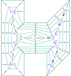
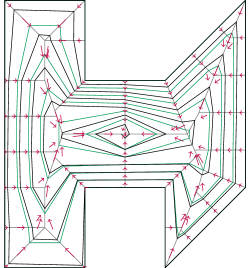
Figure 4: The construction of a polyline spiral in a polygon $\mathcal{P}$: 4 The wavefronts in green and blue arrows from each wavefront corner $\texttt{Wf}[i][w]$ to its parent $\texttt{Wf}[i-1][\texttt{Pa}\texttt{Wf}[i][w]]$. The diagram $\mathcal{VD}$ is in gray. 4 The polyline spiral in black obtained by interpolating between the wavefronts. The purple arrows are from each corner $\texttt{Sp}[i]$ of the spiral to its parent $\texttt{Sp}[\texttt{Pa}[i]]$.

We make a spiral with $r=\lceil\frac{0pt[\texttt{Root}]}{\delta^{\prime}}\rceil$ revolutions, where $\delta^{\prime}=0.95\cdot\delta$. We use the slightly smaller stepover $\delta^{\prime}$ so that the maximum distance between two neighboring revolutions is smaller. That gives more flexibility to smooth the spiral later on as described in section 2.9. We set $\Delta=1/r$ and compute a wavefront for each of the times $\{0,\Delta,2\Delta,\ldots,r\Delta\}$. The two-dimensional array Wf stores the wavefronts, so that the wavefront at time $i\Delta$ is the array $\texttt{Wf}[i]$. Wavefront $i$ is constructed by traversing $\mathcal{VD}$ once and finding every point on $\mathcal{VD}$ with time $i\Delta$ in counterclockwise order. Let $e$ be an edge we have not visited before, and let $n=\texttt{Start}[e]$ and $m=\texttt{End}[e]$. There is a corner of wavefront $i$ on $e$ if $\texttt{TmNd}[n]<i\Delta\leq\texttt{TmNd}[m]$. If that is the case, we add $\texttt{GetPt}(e,i\Delta)$ to the end of $\texttt{Wf}[i]$. We make one corner in $\texttt{Wf}[0]$ for each of the child edges of the root, $\texttt{ChildEs}[\texttt{Root}]$, and all these corners are copies of the point $\texttt{Pt}[\texttt{Root}]$. Using this construction, there is exactly one corner of each wavefront on each path from Root to a leaf of $\mathcal{VD}$.

For each corner $\texttt{Wf}[i][w]$, we store the length of the part of the wavefront up to the corner, i.e. $\texttt{Wf}\texttt{Lng}[i][0]=0$ and

$$\texttt{Wf}\texttt{Lng}[i][w]=\sum_{j=1}^{w}\lVert\texttt{Wf}[i][j]-\texttt{Wf}[i][j-1]\rVert,$$

for $w\geq 1$. Here $\lVert\cdot\rVert$ is the Euclidean norm. We also store the total length of $\texttt{Wf}[i]$ as $\texttt{Ttl}\texttt{Wf}\texttt{Lng}[i]$.

We introduce a rooted tree with the wavefront corners as the nodes. See figure 4. The parent of a corner $\texttt{Wf}[i][w]$, $i>0$, is the unique corner $\texttt{Wf}[i-1][pw]$ on wavefront $i-1$ on the path from $\texttt{Wf}[i][w]$ to Root. We store $pw$ as $\texttt{Pa}\texttt{Wf}[i][w]$, i.e., the parent of $\texttt{Wf}[i][w]$ is $\texttt{Wf}[i-1][\texttt{Pa}\texttt{Wf}[i][w]]$.

Since the distance from each wavefront corner to each of its children is at most $\delta^{\prime}$, the Hausdorff distance between two neighboring wavefronts is also at most $\delta^{\prime}$. Furthermore, since the wave is moving with positive speed towards the leafs of $\mathcal{VD}$ and the faces into which $\mathcal{VD}$ divides $\mathcal{P}$ are convex, neighboring wavefronts do not intersect each other. From the order in which the corners of a wavefront is constructed, it is also clear that a wavefront does not intersect itself.

2.6 Interpolating between the wavefronts

We construct a polyline spiral stored as an array Sp. For each $i=1,\ldots,r$, we construct one revolution of the spiral by interpolating between wavefront $i-1$ and wavefront $i$. Every corner of the spiral is a point on $\mathcal{VD}$. There is exactly one spiral corner on the path in $\mathcal{VD}$ from each wavefront corner $\texttt{Wf}[i][w]$ to its parent $\texttt{Wf}[i-1][\texttt{Pa}\texttt{Wf}[i][w]]$. Assume for now that we know how to choose the actual corners of the polyline spiral. We shall get back to this shortly.

The first corner $\texttt{Sp}[0]$ is on the root node of $\mathcal{VD}$, and for every other corner $\texttt{Sp}[s]$, $s>0$, we store an index of the parent $\texttt{Pa}[s]$, such that the parent $\texttt{Sp}[\texttt{Pa}[s]]$ is the first corner we meet on the path in $\mathcal{VD}$ from $\texttt{Sp}[s]$ to the root. Figure 4 shows the resulting polyline spiral and the parents of each corner. We define the spiral such that the distance between a spiral corner and its parent is at most $\delta^{\prime}$. It follows that the distance from a point on the polyline spiral to the neighboring revolutions is at most $\delta^{\prime}$.

Here we describe how to define the Pa-pointers. When we have constructed a spiral corner $\texttt{Sp}[s]$ which is on the path from $\texttt{Wf}[i][w]$ to its parent wavefront corner $\texttt{Wf}[i-1][pw]$, we know that the first spiral corner on the path from $\texttt{Wf}[i][w]$ to the root is $\texttt{Sp}[s]$, and we store this information as $\texttt{Pa}\texttt{Sp}[i][w]=s$. Therefore, when we have made a new spiral corner $\texttt{Sp}[r]$ on the path from $\texttt{Wf}[i+1][w^{\prime}]$ to its parent $\texttt{Wf}[i][pw^{\prime}]$, the parent of $\texttt{Sp}[r]$ is defined to be $\texttt{Pa}[r]=\texttt{Pa}\texttt{Sp}[i][pw^{\prime}]$. By doing so, the corner $\texttt{Sp}[\texttt{Pa}[r]]$ will be the first spiral corner on the path from $\texttt{Sp}[r]$ to the root.

In the following we describe how to choose the corners of the polyline spiral. We assume that we have finished the revolution of the spiral between wavefronts $i-2$ and $i-1$ and we show how to make the revolution between wavefronts $i-1$ and $i$. For each wavefront corner $\texttt{Wf}[i][w]$, we find the point $\texttt{Q}[w]$ on the path to $\texttt{Wf}[i-1][pw]$, where $pw=\texttt{Pa}\texttt{Wf}[i][w]$, with time

$$t_{w}=(i-1)\Delta+\frac{\texttt{Wf}\texttt{Lng}[i][w]}{\texttt{Ttl}\texttt{Wf}\texttt{Lng}[i]}\Delta.$$

If $\texttt{Q}[w]$ is more than $\delta^{\prime}$ away from $\texttt{Sp}[\texttt{Pa}\texttt{Sp}[i-1][pw]]$, we redefine $\texttt{Q}[w]$ to be the point on the same path with distance exactly $\delta^{\prime}$. We mark the path from $\texttt{Q}[w]$ to the root of $\mathcal{VD}$. See figure 5.

When we have done the marking for each $w$, we traverse wavefront $i$ once more. For each wavefront corner $\texttt{Wf}[i][w]$, we find the first marked point on the path to the root. We let $\texttt{P}[w]$ be that point and $\texttt{T}[w]=\theta(\texttt{P}[w])$ be its time. We have that $\texttt{T}[w]\geq t_{w}$, because a later wavefront corner $\texttt{Wf}[i][w^{\prime}]$, $w^{\prime}>w$, can mark more of the path from $\texttt{Wf}[i][w]$ to the root. Therefore, we can have $\texttt{P}[w]=\texttt{P}[w+1]$ for some $w$. Using this construction, there is exactly one distinct P-point on each path from a wavefront corner to the root. Furthermore, we know that the distance from $\texttt{P}[w]$ to the spiral corner $\texttt{Sp}[\texttt{Pa}\texttt{Sp}[i-1][\texttt{Pa}\texttt{Wf}[i][w]]]$ is at most $\delta^{\prime}$.

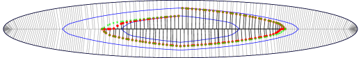
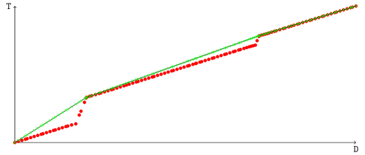
Figure 5: 5 The interpolation between the two blue wavefronts. The boundary $\mathcal{P}$ is in black and the diagram $\mathcal{VD}$ is in gray. The red circles are the points $\texttt{Q}[w]$ and the marked part of of $\mathcal{VD}$ is in black. The green crosses are the resulting points of the polyline spiral stored in Sp after the convexification process. 5 Related values for the same interpolation: The points $(\texttt{D}[w],\texttt{T}[w])$ are red circles. The upper convex hull $\mathcal{F}$ of the points is a black curve, and the green crosses are the points $(\texttt{D}[w],\mathcal{F}(\texttt{D}[w]))$ on that hull.

The polyline defined by the points $\texttt{P}[0],\texttt{P}[1],\ldots$ is basically our interpolated spiral, but the points have a tendency to have unnecessarily sharp corners if $\mathcal{VD}$ is relatively dense, which is often the case for polygons $\mathcal{P}$ occurring in real-world problems. To avoid unnecessary sharp corners, we apply a method which we denote as the convexification, see figure 5. Let $\texttt{D}[w]=\sum_{v=0}^{w-1}\lVert\texttt{P}[v]-\texttt{P}[v+1]\rVert$ be the length of the polyline until $\texttt{P}[w]$ and consider the points $(\texttt{D}[w],\texttt{T}[w])$. We compute the upper convex hull of these points, e.g. using the method of Graham and Yao [6]. Let $\mathcal{F}$ be the function whose graph is the upper hull. By definition, we have that $\texttt{T}[w]\leq\mathcal{F}(\texttt{D}[w])$ for each $w=0,\ldots$. We now choose the corners of Sp in the following way: For each wavefront corner $\texttt{Wf}[i][w]$ in order, we find the point $S$ on the path to the root with time $\mathcal{F}(\texttt{D}[w])$. If $S$ is more than $\delta^{\prime}$ away from the parent spiral corner $\texttt{Sp}[\texttt{Pa}\texttt{Sp}[i-1][\texttt{Pa}\texttt{Wf}[i][w]]]$ (which will be the parent of the spiral corner we are constructing), we choose instead $S$ to be the point on the same path which is exactly $\delta^{\prime}$ away. To avoid repetitions of the same point in Sp, we add $S$ to the end of Sp if $S$ is different from the last point in Sp. Since we get the spiral corners by moving the P-points closer to wavefront $i$, we get exactly one distinct spiral corner on each path from a wavefront corner to the root. When $\mathcal{VD}$ is sparse like in figure 4, the convexification makes no visible difference between the P-points and the final points in Sp, but when $\mathcal{VD}$ is dense as in figure 5, the effect is significant.

We also add one revolution around $\mathcal{P}$ to the end of Sp, which is used to test that the last interpolated revolution respects the stepover when the spiral is rounded later on.

The polyline spiral constructed as described clearly satisfies that the distance from a point on one revolution to the neighboring revolutions is at most $\delta^{\prime}$. Furthermore, each revolution is between two neighboring wavefronts since all the corners of the interpolation between wavefronts $i$ and $i+1$ have times in the interval $\left[i\Delta,(i+1)\Delta\right[$. The wavefronts do not intersect as mentioned earlier, so different revolutions of the polyline spiral do not either. It is also clear from the construction that one revolution does not intersect itself. Therefore, the polyline spiral has all the properties that we require of our spiral except being $G^{1}$ continuous. How to obtain that is described in section 2.9.

2.7 Enriching the diagram

In this and the following section, we describe some modifications we make on the Voronoi diagram of $\mathcal{P}$ before doing anything else. The result is the diagram $\mathcal{VD}=\mathcal{VD}(\mathcal{P})$. Long edges on $\mathcal{P}$ lead to long faces in the Voronoi diagram, so that the wave is not moving towards the boundary $\partial\mathcal{P}$ in a natural way, see figure 2. In figure 2, the wave starts on a long edge, and the first three wavefronts are all degenerated polygons with only two corners, both on the edge. Therefore, we need edges going directly to the boundary with a distance to each other of at most $\delta$, so that each wavefront has corners on more edges than the previous one. We have obtained this by traversing the Voronoi diagram and inspecting each pair of consecutive leafs $l_{1}$ and $l_{2}$. Such a pair of nodes are on the same or on two neighboring corners of $\mathcal{P}$. Assume the latter, so that there is a segment $S$ on $\partial\mathcal{P}$ from $l_{1}$ to $l_{2}$ and a face $f$ of the Voronoi diagram to the left of $S$. Let $s=\texttt{Pt}[l_{2}]-\texttt{Pt}[l_{1}]$ be the vector from $l_{1}$ to $l_{2}$, $d=\lVert s\rVert$ be the length of $S$ and $m=\lceil d/\delta\rceil$. We want to subdivide $f$ into $m$ faces. Let $p_{i}=\texttt{Pt}[l_{1}]+s\cdot\frac{i}{m}$, $i=1,\ldots,m-1$, be interpolated points on $S$. Let $h_{i}=\overrightarrow{p_{i},p_{i}+\widehat{s}}$ be the half-line starting at $p_{i}$ with direction $\widehat{s}$, where $\widehat{s}$ is the counterclockwise rotation of $s$. For each $i=1,\ldots,m-1$, we find the first intersection point between $h_{i}$ and the Voronoi diagram. Assume the intersection for some $i$ is a point $q$ on an edge $e$. If the smallest angle between $h_{i}$ and $e$ is larger than 50 degrees, we split $e$ into two edges by introducing a node at $q$ and add a segment from that node to a new node at $p_{i}$. If the smallest angle is less than 50 degrees, the Voronoi diagram is moving fast enough towards the boundary so that the wavefronts will be fine in that area without adding any additional edges. Figure 1 shows the result of enriching the Voronoi diagram shown in figure 1.

2.8 Removing double edges to concave corners

A concave corner of $\mathcal{P}$ is a corner where the inner angle is more than 180 degrees. Each concave corner $c$ on $\mathcal{P}$ leads to a face in the Voronoi diagram of all the points in $\mathcal{P}$ being closer to $c$ than to anything else on the boundary of $\mathcal{P}$. Therefore, there are two edges $e_{1}$ and $e_{2}$ of the Voronoi diagram with an endpoint on $c$. We have found that we get a better spiral if we remove these edges and instead add an edge following the angle bisector of the edges, i.e., we follow the bisector from $c$ and find the first intersection point $q$ with the Voronoi diagram and add an edge from $q$ to $c$, see figure 1. The reason that this process improves the resulting spiral is that the wavefronts will resemble $\mathcal{P}$ more because they will have one corner on the bisector edge corresponding to the corner $c$ on $\mathcal{P}$. We can only do this manipulation if the resulting faces are also convex. That is checked easily by computing the new angles of the manipulated faces and it seems to be the case almost always.

2.9 Rounding the polyline spiral

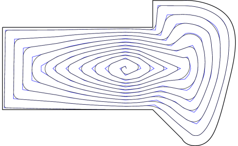
Figure 6: The spirals from figure 3 together. The polyline spiral is blue and the rounded spiral is black.

In this section we describe a possible way for smoothing the polyline spiral to get a $G^{1}$ continuous spiral. See figure 6 for a comparison between the rounded and unrounded spiral from figure 3 using this method. Note that some of the arcs of the rounded spiral rounds multiple corners of the polyline spiral.

For each corner on the polyline spiral, we substitute a part of the spiral containing the corner with a circular arc which is tangential to the polyline spiral in the endpoints. That gives a spiral which is $G^{1}$ continuous, i.e., having no sharp corners. Each arc is either clockwise or counterclockwise. For each index $i$, let $s_{i}=\texttt{Sp}[i]\texttt{Sp}[i+1]$ be the segment from $\texttt{Sp}[i]$ to $\texttt{Sp}[i+1]$ and $v_{i}=\texttt{Sp}[i+1]-\texttt{Sp}[i]$ be the vector from $\texttt{Sp}[i]$ to $\texttt{Sp}[i+1]$. Each arc has the startpoint $p$ on some segment $s_{a}$ and the endpoint $q$ on another segment $s_{b}$, $a<b$, so that the arc substitutes the part of the polyline spiral from $p$ to $q$. We say that the arc rounds the corners $a+1$ to $b$. We call the arc tangential if it is counterclockwise and its center is on the intersection of the half-lines $\overrightarrow{p,p+\widehat{v_{s}}}$ and $\overrightarrow{q,q+\widehat{v_{r}}}$ or it is clockwise and its center is on the intersection of the half-lines $\overrightarrow{p,p-\widehat{v_{s}}}$ and $\overrightarrow{q,q-\widehat{v_{r}}}$.

We store a pointer $\texttt{Arc}[i]$ to the arc that substitutes the corner $\texttt{Sp}[i]$. The same arc can substitute multiple consecutive corners, so that $\texttt{Arc}[i]=\texttt{Arc}[i+1]=\ldots=\texttt{Arc}[i+k-1]$. In that case, when $\texttt{Arc}[i-1]\neq\texttt{Arc}[i]\neq\texttt{Arc}[i+k]$, the neighbors of $\texttt{Arc}[i]$ are $\texttt{Arc}[i-1]$ and $\texttt{Arc}[i+k]$. Two different arcs must substitute disjoint parts of the polyline spiral for the rounded spiral to be well-defined. We subdivide each segment $s_{a}$ at a point $p_{a}\in s_{a}$ such that an arc ending at $s_{a}$ must have its endpoint at the segment $\texttt{Sp}[a]p_{a}$ and an arc beginning at $s_{a}$ must have its startpoint on the segment $p_{a}\texttt{Sp}[a+1]$. The point $p_{a}$ is chosen as a weighted average of $\texttt{Sp}[a]$ and $\texttt{Sp}[a+1]$ so that the arc rounding the sharpest of the corners $\texttt{Sp}[a]$ and $\texttt{Sp}[a+1]$ gets most space. Let $\phi_{a}\in(-\pi,\pi]$ be the angle at corner $\texttt{Sp}[a]$ of the polyline spiral. We set $w_{a}=\frac{\pi-\phi_{a}}{2\pi-\phi_{a}-\phi_{a+1}}$ and choose $p_{a}$ as $p_{a}=(1-w_{a})\cdot\texttt{Sp}[a]+w_{a}\cdot\texttt{Sp}[a+1]$.

We keep a priority queue $Q$ [4] of the arcs that can possibly be enlarged. After each enlargement of an arc, the resulting spiral respects the stepover $\delta$ and no self-intersection has been introduced. We say that an arc with these properties is usable. Initially, we let each corner be rounded by a degenerated zero-radius arc, and $Q$ contains all these arcs. Clearly, these initial zero-radias arcs are usable by definition. We consider the front arc $A$ in $Q$ and try to find another usable arc $A^{\prime}$ that substitutes a longer chain of the polyline spiral. The new arc $A^{\prime}$ normally has a larger radius than $A$. If possible, we choose $A^{\prime}$ so that it also substitutes one or, preferably, two of the neighbors of $A$. Assume that we succeed in making a usable arc $A^{\prime}$ substituting both $A$ and its neighbors $B$ and $C$. Now $A^{\prime}$ rounds the union of the corners previously rounded by $A$, $B$, and $C$. For all these corners, we update the Arc-pointers and we remove $A$, $B$, and $C$ from $Q$. We add $A^{\prime}$ to $Q$. For every corner that $A^{\prime}$ rounds, we also add the arcs rounding the children and parents of that corner to $Q$, since it is possible that these arcs can now be enlarged. If no larger usable arc $A^{\prime}$ is found, we just remove $A$ from $Q$. The rounding process terminates when $Q$ is empty.

We test if an arc is usable by measuring the distance to the arcs rounding the child and parent corners. That is easily done using elementary geometric computations.

Here we describe how to find the largest usable arc rounding the corners $a+1$ to $b$, $a<b$. We find the possible radii of tangential arcs beginning at a point on $p_{a}\texttt{Sp}[a+1]$ and ending at a point on $\texttt{Sp}[b]p_{b}$ using elementary geometry. There might be no such arcs, in which case we give up finding an arc rounding these corners. Otherwise, we have an interval $[r_{\min},r_{\max}]$ of radii of tangential arcs going from $p_{a}\texttt{Sp}[a+1]$ and ending on $\texttt{Sp}[b]p_{b}$. We check if the arc with radius $r_{\min}$ is usable. If it is not, we give up. Otherwise, we check if the arc with radius $r_{\max}$ is usable. If it is, we use it. Otherwise, we make a binary search in the interval $[r_{\min},r_{\max}]$ after the usable arc with the largest radius. We stop when the binary search interval has become sufficiently small, for instance $0.01\cdot\delta$, and use the arc with the smallest number in the interval as its radius.

The order of the arcs in $Q$ is established in the following way: We have found that giving the arc $A$ the priority $P(A)=r(A)/r(C_{\max})+1/s(A)$ gives good results, where $r(A)$ is the radius of $A$, $s(A)$ is the size of the subtended angle from the center of $A$ in radians, and $r(C_{\max})$ is the radius of the maximum circle contained in $\mathcal{P}$. The front arc in $Q$ is the one with smallest $P$-value. We divide by $r(C_{\max})$ to make the rounding invariant when $\mathcal{P}$ and $\delta$ are scaled by the same number. $r(C_{\max})$ can be obtained from the Voronoi diagram of $\mathcal{P}$, since the largest inscribed circle has its center on a node in the diagram. If $s(A)=0$, we set $P(A)=\infty$, since there is no corner to round.

We see that arcs with small radii or large subtended angles are chosen first for enlargement. In the beginning when all the arcs in $Q$ have zero radius, the arcs in the sharpest corners are chosen first because their degenerated arcs have bigger subtended angles – even though the radius is zero, we can still define the start and end angle of the arc according to the slope of the segments meeting in the corner and thus define the subtended angle of the arc.

If two or three arcs are substituted by one larger arc each time we succeed in making a larger arc, we are sure that the rounding process does terminate, since the complexity of the spiral decreases. However, it is often not possible to merge two or three arcs, but only to make a larger arc rounding the same corners as an old one. The rounded spiral gets better, but we cannot prove that the process terminates. In practice, we have seen fast termination in any tested example. A possible remedy could be only to allow each arc to increase in size without rounding more corners a fixed number of times.

3 Computing a spiral in a pocket with an island

In many practical applications, the area to be machined is not simply-connected, but has one or more “islands” that should not be machined. It might be because there are physical holes in the part or areas of a thicker layer of material not to be machined in the same depth. Therefore, assume that we are given a polygon $\mathcal{P}$ and a single polygonal island $\mathcal{I}$ in the interior of $\mathcal{P}$. In section 5 we suggest a method to deal with multiple islands. By $\mathcal{P}\setminus\mathcal{I}$, we denote the closed set of points which are in the interior or on the boundary of $\mathcal{P}$ but not in the interior of $\mathcal{I}$. We want to compute a spiral which is contained in $\mathcal{P}\setminus\mathcal{I}$ such that the Hausdorff distance is at most $\delta$ between (i) two consecutive revolutions, (ii) $\partial\mathcal{I}$ and the first revolution, and (iii) $\partial\mathcal{P}$ and the last revolution. As before, $\delta$ is the user-defined stepover. We also require that the spiral is $G^{1}$ continuous and has no self-intersections. See figure 7 for an example.

As in the case with a simply-connected pocket, we use a wave model to construct the spiral. We imagine a wave that has exactly the shape of $\partial\mathcal{I}$ at time $0$ and moves towards $\partial\mathcal{P}$, so that at the time $1$, it reaches $\partial\mathcal{P}$ everywhere. We explain how to define a polyline spiral. The spiral should be rounded by a method similar to the one described in section 2.9.

3.1 The Voronoi diagram of a pocket with an island

We use the Voronoi diagram of the set of line segments of $\mathcal{P}$ and $\mathcal{I}$. As in the case with no islands, we modify the diagram slightly. Let $\mathcal{VD}=\mathcal{VD}(\mathcal{P}\setminus\mathcal{I})$ be the modified polygon. Like the true Voronoi diagram, the modified diagram $\mathcal{VD}$ has the following properties:

• $\mathcal{VD}$ is a connected, plane graph contained in $\mathcal{P}\setminus\mathcal{I}$,

• each leaf of $\mathcal{VD}$ is on the boundary of $\mathcal{P}$ or $\mathcal{I}$,

• there is at least one leaf of $\mathcal{VD}$ on each corner of $\mathcal{P}$ and $\mathcal{I}$,

• all the faces into which $\mathcal{VD}$ divides $\mathcal{P}\setminus\mathcal{I}$ are convex,

• $\mathcal{VD}$ contains exactly one cycle, the cycle is the locus of all points being equally close to $\partial\mathcal{I}$ and $\partial\mathcal{P}$, and $\mathcal{I}$ is contained in its interior.

Figure 7: 7 A polygon $\mathcal{P}$ with an island $\mathcal{I}$, both in black. The diagram $\mathcal{VD}$ of $\mathcal{P}\setminus\mathcal{I}$ is drawn with the cycle $\mathcal{C}$ in blue and the other edges in gray. 7 The resulting spiral.

The diagram $\mathcal{VD}$ is consisting of one cycle $\mathcal{C}$, which we also denote by the central cycle, and some trees growing out from $\mathcal{C}$, see figure 7. Each of the trees grows either outwards and has all its leafs on $\partial\mathcal{P}$ or inwards and has all its leafs on $\partial\mathcal{I}$. The general idea is to use the method described in section 2 to define wavefronts in each of these trees separately. Afterwards, we interpolate between the neighboring wavefronts in each tree and connect the interpolated pieces to get one contiguous spiral.

As in the case of a polygon without an island, we enrich the Voronoi diagram by adding edges equidistantly along and perpendiculairly to long edges on $\partial(\mathcal{P}\setminus\mathcal{I})$ as described in section 2.7. One small difference is that if the half-line $h_{i}$ intersects an edge $e$ at the point $q$, and $e$ is an edge on the cycle $\mathcal{C}$, we do not split $e$ and do not introduce a new edge from $q$ to $p_{i}$. There would be no advantage of adding that edge. We also remove double edges to concave corners and add their bisector instead as described in section 2.8.

We want the trees to be symmetric in the sense that there is a tree $\mathcal{P}\mathcal{T}_{n}$ with root $n\in\mathcal{C}$ and leafs on $\partial\mathcal{P}$ if and only if there is a tree $\mathcal{I}\mathcal{T}_{n}$ with root $n$ and leafs on $\partial\mathcal{I}$. If for a node $n\in\mathcal{C}$ we only have one of the trees, say $\mathcal{I}\mathcal{T}_{n}$, we add an edge from node $n$ to the closest point on $\partial\mathcal{P}$ and let $\mathcal{P}\mathcal{T}_{n}$ be the tree consisting of that single edge. It follows from the properties of the Voronoi diagram that the added edge does not intersect any of the other edges.

We store $\mathcal{C}$ as a vector $[n_{0},\ldots,n_{c-1}]$ of the nodes on $\mathcal{C}$ in counterclockwise order, such that there are trees $\mathcal{I}\mathcal{T}_{n_{i}}$ and $\mathcal{P}\mathcal{T}_{n_{i}}$ for each $i=0,\ldots,c-1$. A root node is a node $n$ on $\mathcal{C}$. We let $\mathcal{T}_{n}=\mathcal{P}\mathcal{T}_{n}\cup\mathcal{I}\mathcal{T}_{n}$ be the union of the two trees rooted at node $n\in\mathcal{C}$ and consider $\mathcal{T}_{n}$ as a tree rooted at node $n$.

3.2 Defining the movement of the wave

On each tree $\mathcal{T}_{n}$ we now define a wave model similar to the one described in section 2.1. The wave starts at time $t=0$ on the leafs on $\partial\mathcal{I}$ and moves through $\mathcal{T}_{n}$ so that it hits the leafs on $\partial\mathcal{P}$ at time $t=1$. Once the time and speed in the node $n$ is determined, the times and speeds on the other nodes and edges in $\mathcal{T}_{n}$ are computed analogously to algorithm 2. One difference is that we compute decreasing times for the tree $\mathcal{I}_{n}$. A way to do so is to set $\texttt{TmNd}[n]=1-\texttt{TmNd}[n]$, compute the inverse times using algorithm 2, and afterwards inverse each of the computed times $t$ by setting $t=1-t$.

Let the preferred time of a node $n$ be $t_{n}=\frac{\texttt{Isl}0pt[n]}{\texttt{Bnd}0pt[n]+\texttt{Isl}0pt[n]}$, where $\texttt{Bnd}0pt[n]$ is the length of the longest path to a leaf in $\mathcal{P}\mathcal{T}_{n}$ and $\texttt{Isl}0pt[n]$ is the length of the longest path to a leaf in $\mathcal{I}\mathcal{T}_{n}$. Similarly, if the time $\texttt{TmNd}[n]$ has already been defined, we let the preferred speed of $n$ be $v_{n}=\max\left\{\frac{\texttt{Isl}0pt[n]}{\texttt{TmNd}[n]},\frac{\texttt{Bnd}0pt[n]}{1-\texttt{TmNd}[n]}\right\}$.

A naive method to define the times and speeds of a root $n$ is to set $\texttt{TmNd}[n]=t_{n}$ and $\texttt{VeNd}[n]=v_{n}$. That will minimize the number of revolutions and give the most equidistant wavefronts on each tree $\mathcal{T}_{n}$. However, the abrupt changes in time and speed along the central cycle $\mathcal{C}$ results in a spiral which curves a lot. Instead, we might smooth the times and speeds around $\mathcal{C}$. See figure 8 for a comparison of the wavefronts with and without smoothing. There may be many ways of smoothing the values. After much experimentation, we have found the method described in B to give good results. Notice that the wavefronts in figure 8 intersect each other, and that will indeed also be the case for some problem instances after using the smoothing method described in B. However, in the end of section 3.4 we describe how to ensure that the polyline spiral will not have any self-intersections.

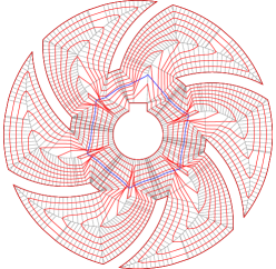
Figure 8: 7 Wavefronts in red when the times and speeds of the wave in the root nodes have been defined as described in B. $\mathcal{C}$ is in blue and the rest of $\mathcal{VD}$ is in gray. 8 Wavefronts when the preferred times and speeds have been used to define the movement of the wave.

3.3 Creating wavefronts

For a given root node $n\in\mathcal{C}$, we want at least $s_{\mathcal{I}_{n}}=\frac{\texttt{Isl}0pt[n]}{\delta^{\prime}}$ revolutions of the spiral in the tree $\mathcal{I}\mathcal{T}_{n}$ in order to respect the stepover $\delta^{\prime}=0.95\cdot\delta$. Similarly, we want $s_{\mathcal{P}_{n}}=\frac{\texttt{Bnd}0pt[n]}{\delta^{\prime}}$ revolutions in $\mathcal{P}\mathcal{T}_{n}$. Therefore, the time between two revolutions should be at most $\Delta_{n}=\min\{\frac{\texttt{TmNd}[n]}{s_{\mathcal{I}_{n}}},\frac{1-\texttt{TmNd}[n]}{s_{\mathcal{P}_{n}}}\}$. Hence, we let $\Delta^{\prime}=\min_{n\in\mathcal{C}}\{\Delta_{n}\}$ be the minimum over all such values. We let the number of revolutions be $r=\lceil 1/\Delta^{\prime}\rceil$ and set $\Delta=1/r$.

Each tree $\mathcal{T}_{n}$ contains a contiguous subset of the corners of any wavefront $i$. The corners of the subset are points on $\mathcal{I}\mathcal{T}_{n}$ if and only if $t\leq\texttt{TmNd}[n]$, otherwise they are on $\mathcal{P}\mathcal{T}_{n}$. Let $r_{n}=\lfloor\frac{\texttt{TmNd}[n]}{\Delta}\rfloor$. The wavefronts $i=0,\ldots,r_{n}$ are on $\mathcal{I}\mathcal{T}_{n}$, while wavefronts $i=r_{n}+1,\ldots,r$ are on $\mathcal{P}\mathcal{T}_{n}$. As explained in section 3.2, we do not use the same time $\texttt{TmNd}[n]$ for every node $n$ on $\mathcal{C}$. Therefore, we may get wavefronts crossing $\mathcal{C}$, as is seen in figure 8.

We suggest to store the wavefront corners in a two-dimensional array for each of the trees $\mathcal{I}\mathcal{T}_{n}$ and $\mathcal{P}\mathcal{T}_{n}$. The wavefront corners on $\mathcal{I}\mathcal{T}_{n}$ of one wavefront are stored in an array $\texttt{Isl}\texttt{Wf}[n][j]$, where index $j$ corresponds to wavefront $i=r_{n}-j+1$. In $\mathcal{P}\mathcal{T}_{n}$, the array $\texttt{Bnd}\texttt{Wf}[n][j]$ stores corners of wavefront $i=j+r_{n}$. Hence, the corners of each wavefront is stored locally in each tree $\mathcal{T}_{n}$.

In $\mathcal{I}\mathcal{T}_{n}$, the parents of the corners of wavefront $i=0,\ldots,r_{n}-1$ are corners of wavefront $i+1$. In $\mathcal{P}\mathcal{T}_{n}$, the parents of the corners of wavefront $i=r_{n}+2,\ldots,r$ are corners of wavefront $i-1$. Therefore, all parents are on the wavefront one step closer to the root $n$. In both $\mathcal{I}\mathcal{T}_{n}$ and $\mathcal{P}\mathcal{T}_{n}$, we introduce fake wavefront corners at node $n$ stored in the arrays $\texttt{Isl}\texttt{Wf}[n][0]$ and $\texttt{Bnd}\texttt{Wf}[n][0]$, respectively, which are the parents of the corners in the arrays $\texttt{Isl}\texttt{Wf}[n][1]$ and $\texttt{Bnd}\texttt{Wf}[n][1]$. Thus, these fake corners are not corners on wavefront $i$ for any $i=0,\ldots,r$, but are merely made to complete the tree of parent pointers between corners of neighboring wavefronts.

We also need an array WfLng containing global information about the length of each wavefront crossing all the trees $\{\mathcal{T}_{n}\}_{n}$ in order to do interpolation between the wavefronts later. We have $\texttt{Wf}\texttt{Lng}[i][0]=0$ for every wavefront $i$. If $c_{m}$ and $c_{m+1}$ are the $m$’th and $(m+1)$’st corners on wavefront $i$, respectively, we have $\texttt{Wf}\texttt{Lng}[i][m+1]=\texttt{Wf}\texttt{Lng}[i][m]+\lVert c_{m+1}-c_{m}\rVert$. Notice that $c_{m}$ and $c_{m+1}$ can be corners in different, however neighbouring trees $\mathcal{T}_{n}$ and $\mathcal{T}_{n^{\prime}}$ and hence stored in different arrays. $\texttt{Ttl}\texttt{Wf}\texttt{Lng}[i]$ stores the total length of wavefront $i$.

3.4 Interpolating between wavefronts

We interpolate between two wavefronts $i-1$ and $i$ in each tree $\mathcal{T}_{n}$ separately, but using the same technique as in section 2.6. If $i\leq r_{n}$, we interpolate between the wavefront fragments stored in $\texttt{Isl}\texttt{Wf}[n][j]$ and $\texttt{Isl}\texttt{Wf}[n][j+1]$, where $j=r_{n}-i+1$, using the values of the length of wavefront $i-1$ stored in $\texttt{Wf}\texttt{Lng}[i-1]$. If $i>r_{n}+1$, we interpolate between $\texttt{Bnd}\texttt{Wf}[n][j-1]$ and $\texttt{Bnd}\texttt{Wf}[n][j]$, where $j=i-r_{n}$, using the values stored in $\texttt{Wf}\texttt{Lng}[i]$. A special case occurs when $i=r_{n}+1$, i.e., when we are interpolating between the first wavefront on each side of the root node $n$. In that case, let

$$t=(i-1)\Delta+\frac{\texttt{Wf}\texttt{Lng}[i][m]}{\texttt{Ttl}\texttt{Wf}\texttt{Lng}[i]}\Delta,$$

when $\texttt{Bnd}\texttt{Wf}[n][1][0]$ is the $m$’th corner on wavefront $i$. If $t\leq\texttt{TmNd}[n]$, we interpolate between $\texttt{Isl}\texttt{Wf}[n][0]$ and $\texttt{Isl}\texttt{Wf}[n][1]$. Otherwise, we interpolate on the other side of $\mathcal{C}$, that is, between $\texttt{Bnd}\texttt{Wf}[n][0]$ and $\texttt{Bnd}\texttt{Wf}[n][1]$. The convexification process described in section 2.6 can be used in each tree $\mathcal{T}_{n}$ separately.

We may store the interpolated spiral in an one-dimensional array Sp. Before we add the first interpolated revolution to Sp, i.e., the one between wavefront $0$ and $1$, we add wavefront $0$ to Sp, that is, all the corners on $\partial\mathcal{I}$. Likewise, after the final revolution between wavefronts $r-1$ and $r$, we add wavefront $r$, which is all the corners on $\partial\mathcal{P}$. These are used to ensure that the distance from the first and last revolution to $\partial\mathcal{I}$ and $\partial\mathcal{P}$, respectively, does respect the stepover when rounding the spiral.

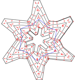
Figure 9: A polyline spiral in black and red arrows from each corner $\texttt{Sp}[s]$ to its parents. The cycle $\mathcal{C}$ is in blue and the diagram $\mathcal{VD}$ is in gray.

For every corner $\texttt{Sp}[s]$ we have a pointer $\texttt{Pa}[s]$ such that $\texttt{Sp}[\texttt{Pa}[s]]$ is the first spiral corner we meet when traveling from $\texttt{Sp}[s]$ to the root $n$ of the tree $\mathcal{T}_{n}$ containing $\texttt{Sp}[s]$. The parents are not defined for the spiral corners closest to the root node $n$. Therefore, we make every spiral corner between $\texttt{Isl}\texttt{Wf}[n][0]$ and $\texttt{Isl}\texttt{Wf}[n][1]$ the parent of every spiral corner between $\texttt{Bnd}\texttt{Wf}[n][0]$ and $\texttt{Bnd}\texttt{Wf}[n][1]$ to make parent dependencies across $\mathcal{C}$. We want all the parent pointers to be towards the island $\mathcal{I}$. Therefore, we reverse all the pointers between pairs of corners in each tree $\mathcal{I}\mathcal{T}_{n}$. Now, the parent pointers are defined for all spiral corners except for the ones on $\partial\mathcal{I}$. See figure 9 for an example of a polyline spiral around an island and red arrows indicating the parent pointers. Notice that a corner can have multiple parents, but the parents are consecutive and can thus be stored using two indices.

In section 2.6, we stated that since there are no intersections between different wavefronts, the polyline spiral has no self-intersections when there is no island in $\mathcal{P}$. The wavefronts do not intersect in that case due to the convexity of the faces into which the diagram $\mathcal{VD}(\mathcal{P})$ subdivides $\mathcal{P}$. When there is an island $\mathcal{I}$ in $\mathcal{P}$, there are two kinds of faces into which $\mathcal{VD}(\mathcal{P}\setminus\mathcal{I})$ subdivides $\mathcal{P}\setminus\mathcal{I}$, see figure 10. Some faces, like $a_{3}$ in the figure, are bounded by edges of one tree $\mathcal{T}_{n}$ while some are between two trees, like $a_{1}$ and $a_{2}$. The latter kind is bounded by edges of two neighboring trees $\mathcal{T}_{n}$ and $\mathcal{T}_{m}$ and an edge $e$ from $n$ to $m$ on $\mathcal{C}$, where $n$ and $m$ are neighboring nodes on $\mathcal{C}$. The first kind of faces is similar to the faces in section 2, so here we do not worry about self-intersections of the spiral. The second, however, can lead to wavefronts crossing each other and therefore also a self-intersecting spiral as is the case in the figure when the spiral jumps over $\mathcal{C}$ and crosses $a_{2}$. If the union of the faces on each side of $e$ is convex, like $a_{1}$ and its neighboring face on the other side of $\mathcal{C}$, there is no problem. It can easily be tested if the union of the faces is convex by considering the angles of the union at nodes $n$ and $m$. If it is not, we introduce a new corner on the edge on $\mathcal{C}$ whenever the spiral jumps from one side of $\mathcal{C}$ to the other. The new corner is an interpolation of nodes $n$ and $m$ using the time of the spiral in the last corner in tree $\mathcal{T}_{n}$. Figure 10 shows the result of introducing the extra corners. Our experience is that these intersection problems occur very rarely when the method described in B has been applied.

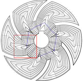
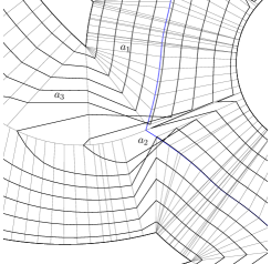
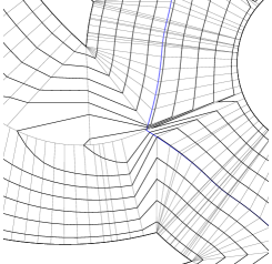
Figure 10: The same pocket and island as in figure 8. The cycle $\mathcal{C}$ is blue, the other edges of $\mathcal{VD}$ are gray. The interpolated spiral is black, and we have not introduced extra spiral corners on $\mathcal{C}$ to avoid self-intersections. In order to emphasize the intersection problems that can arise, we have not used the method described in B, but merely used the preferred time and speed of each node (section 3.2). 10 is a close-up of 10 of the area in the red rectangle. In 10, we have introduced new corners on $\mathcal{C}$ when the spiral jumps from one side of $\mathcal{C}$ to the other when the union of the two faces on each side of $\mathcal{C}$ is not convex.

4 The skeleton method for a spiral in a pocket without an island

Figure 11: Comparison of the basic spiral method from section 2, figure 11, with the improved skeleton method from section 4, figure 11. Note that the spiral obtained from the skeleton method is significantly shorter and that the distance between neighboring revolutions is varying much less than when using the basic method.

The method from section 2 is mainly applicable if the polygon $\mathcal{P}$ is not too far from being a circle. If $\mathcal{P}$ is very elongated or branched, the distance between neighboring revolutions will often be much less than the maximum stepover. Therefore, the toolpath will be unnecessarily long and the cutting width will vary a lot. That leads to long machining time and an uneven finish of the part. See figure 11 for an example. In such cases, we construct a skeleton in $\mathcal{P}$, which is an island $\mathcal{I}$ with zero area. We then use the method from section 3 to make a spiral from the island to the boundary. It does not matter for the construction of the spiral that the island $\mathcal{I}$ has zero area. See figure 11 for a comparison between the basic method from section 2 with the skeleton method described here when applied to the same polygon.

4.1 Constructing the skeleton in a polygon $\mathcal{P}$

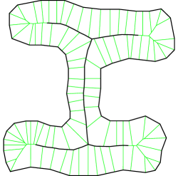
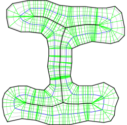
Figure 12: 12 The diagram $\mathcal{VD}(\mathcal{P})$ of the polygon $\mathcal{P}$ from figure 11 in green, where the edges chosen for the skeleton are black. 12 The diagram $\mathcal{VD}(\mathcal{P}\setminus\mathcal{I})$ of $\mathcal{P}$ with the skeleton considered an island $\mathcal{I}$. The cycle $\mathcal{C}$ is blue and the remaining edges are green. The resulting spiral from figure 11 is included in gray.

We choose the skeleton as a connected subset of the edges of the diagram $\mathcal{VD}=\mathcal{VD}(\mathcal{P})$. We traverse $\mathcal{VD}$ once starting at the root and decide for each edge whether to include it in the skeleton. If an edge from node $n$ to $m$ is not included, we don’t include anything from the sub-tree $\mathcal{VD}[m]$. For any node $n$, let $d(n)$ be the length of the shortest path from $n$ to a leaf in $\mathcal{VD}[n]$, and let $D=\max_{n\in\mathcal{VD}}d(n)$. We have found that the following criteria for including an edge $e$ from node $n$ to $m$ gives good results. We require all the criteria to be satisfied.

1. The longest path from $n$ to a leaf in $\mathcal{VD}[n]$ goes through $m$ or $\ell[e]+0pt[m]\geq 1.5\cdot D$, where $\ell[e]$ is the length of edge $e$.

2. The length of the spanned boundary (defined in B) of $m$ is larger than $2\cdot D$.

3. $0pt[m]\geq D$.

Criterion 1 is to avoid getting a skeleton that branches into many short paths. Therefore, we only make a branch which is not following the longest path from $n$ if it seems to become at least $0.5\cdot D$ long (taking criterion 3 into account). When criterion 2 fails, it seems to be a good indicator that an edge is not a significant, central edge in $\mathcal{VD}$, but merely one going straight to the boundary. Criterion 3 ensures that we do not get too close to the boundary. If we did, we would get very short distances between the neighboring revolutions there. If criterion 3 is the only failing criterion, we find the point $p$ on $e$ such that $0pt[m]+\lVert p-\texttt{Pt}[m]\rVert=D$ and include the edge from node $n$ to $p$ in the skeleton. See figure 12 for the skeleton constructed given the polygon from figure 11.

If the polygon is close to being a circle, the method described here results in a very small skeleton, and we get a better spiral using the basic method from section 2 in that case. This can be tested automatically by falling back to the basic method if the circumference of the skeleton is less than, say, 5% of the circumference of $\mathcal{P}$.

5 Computing a spiral in a pocket with multiple islands

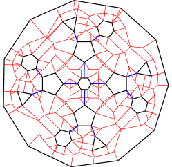
Figure 13: 13 A polygon with 13 islands. The bridges chosen among the Voronoi edges to connect the islands are blue. The remaining Voronoi edges are red. 13 The resulting spiral around the islands.

The method from section 3 works only for polygons with a single island. If there are many islands $\mathcal{I}_{0},\ldots,\mathcal{I}_{h-1}$ in a polygon $\mathcal{P}$, we may connect them with bridges in a tree structure to form one big connected island, see figure 13. The basic idea of reducing the number of islands by connecting them is also used by Chuang and Yang [3] and Held and Spielberger [11]. Our method is given in algorithm 1, and it is a variation of the minimum spanning tree algorithm of Dijkstra [5]. We choose the bridges as edges in the Voronoi diagram $V$ of the area $\mathcal{P}\setminus\bigcup_{i=0}^{h-1}\mathcal{I}_{i}$. The algorithm creates an array Bridges of the edges to use as bridges. We keep a growing set $s$ of the nodes of the Voronoi diagram that we have connected by bridges so far. Here, we have represented $s$ as a bit-vector. We first find one central node $n_{0}$ and $s$ is only containing $n_{0}$ in the beginning. We use Dijkstra’s algorithm [5] in the loop beginning at line 1 to make all shortest paths from nodes in $s$. We make a relaxation of the distances in line 1. When we reach an island $\mathcal{I}_{i}$ whose corners are not in $s$, we use the shortest path to that island as a bridge and add the nodes on the shortest path and the corners on $\mathcal{I}_{i}$ to $s$. The use of the distance vector $d$ makes the algorithm prefer to build bridges from the vertices that has been in $s$ for the longest time. That makes the bridges grow from the center node $n_{0}$ out in every direction. If we did not choose the bridges in this careful way, the resulting connected island would possibly make unnecessarily long dead ends that would require many revolutions to fill out by the spiral.

VRONI by Held [8] has the possibility to add edges to the Voronoi diagram between neighboring objects in the input where the distance between the objects is shortest, even though these are not genuine Voronoi edges. It is an advantage also to consider these edges when choosing the bridges between the islands, since they are often the best bridges. For instance, all the bridges chosen in the example of figure 13 are of that kind.

1 Compute the Voronoi diagram $V$ of the area inside $\mathcal{P}$ but outside every $\mathcal{I}_{i}$.

2 Find the set of all nodes $N$ of $V$ which are either a corner on an island or equally close to two islands but farther from $\partial\mathcal{P}$.

3 Let $n_{0}$ be the node in $N$ closest to the root of $\mathcal{VD}(\mathcal{P})$ defined as in section 2.2.

4 Let $s[n]\leftarrow\texttt{FALSE}$ for each node $n\in V$.

5 Let $d[n]\leftarrow\infty$ for each node $n\in V$.

6 $s[n_{0}]\leftarrow\texttt{TRUE}$; $d[n_{0}]\leftarrow 0$

7 $\texttt{Bridges}\leftarrow[\;]$

8 while $s$ does not include every island do

9       For each node $n$, if $s[n]=\texttt{FALSE}$, set $d[n]=\infty$.

10       Let $p[n]=\texttt{NULL}$ for each node $n$.

11       Let $Q$ be a priority queue of the nodes $n$ of $V$ sorted after the values $d[n]$.

12       while $Q\neq\emptyset$ do

13             Let $n$ be the front node in $Q$ and remove $n$ from $Q$.

14             if $n$ is a corner on an island $\mathcal{I}_{i}$ and $s[n]=\texttt{FALSE}$ 

15                   For each node $n^{\prime}$ on the path $n,p[n],p[p[n]],\ldots$, set $s[n^{\prime}]\leftarrow\texttt{TRUE}$.

16                   Add each edge on the path $n,p[n],p[p[n]],\ldots$ to Bridges.

17                   Let $n_{f}$ be the node on $\mathcal{I}_{i}$ farthest from $n$ and let $a\leftarrow\lVert n_{f}-n\rVert$.

18                   For each node $n^{\prime}$ on $\mathcal{I}_{i}$, set $d[n^{\prime}]\leftarrow d[n]+a$ and $s[n^{\prime}]\leftarrow\texttt{TRUE}$.

19                   Go to line 1.

20                  

21            For each edge going out of $n$ to a node $n^{\prime}\in V$, if $s[n^{\prime}]=\texttt{FALSE}$ and $d[n]+\lVert n-n^{\prime}\rVert<d[n^{\prime}]$, set $d[n^{\prime}]\leftarrow d[n]+\lVert n-n^{\prime}\rVert$, update $Q$ accordingly, and set $p[n^{\prime}]\leftarrow n$.

22            

23      

Algorithm 1 $\texttt{Make}\texttt{Bridges}(\mathcal{P},\mathcal{I}_{0},\ldots,\mathcal{I}_{h-1})$

6 Conclusion

We have described methods for the computation of spiral toolpaths suitable for many shapes of pockets for which no previously described algorithms yield equally good results. Our main contribution is the new possibility of making a spiral morphing an island in a pocket to the boundary of the pocket.

Our developed spiral algorithms only work for polygonal input. We believe that it should be possible to generalize to input consisting of line segments and circular arcs, as done by Held and Spielberger [10], using ArcVRONI by Held and Huber [9] to compute the Voronoi diagrams for such input.

Held and Spielberger [11] developed methods to subdivide a pocket with arbitrarily many islands into simply-connected sub-pockets, each of which are suitable for basic spirals as the ones described in section 2. Since we have the possibility to make spirals around islands, we never have to partition the input into separate areas, but in some cases, for instance if the pocket has a long “arm” requiring a lot of revolutions, it might be useful to machine different areas of the input independently. Another possibility is to combine the method for machining around multiple islands with the skeleton method. Given these new possibilities, our problem is quite different from the one discussed by Held and Spielberger. It would be interesting to investigate if and how one can make an automatic partitioning that leads to a more efficient toolpath using our new kinds of spirals.

Appendix A An algorithm defining the movement of the wave

Here we describe how we define the speed and time of the wave at every point in the diagram $\mathcal{VD}(\mathcal{P})$ in a polygon $\mathcal{P}$ with no island. There might be other models giving equally good or even better results, but we think this model has an advantage of being quite simple to implement. Recall that for a node $n$ in the diagram $\mathcal{VD}$, $\texttt{TmNd}[n]$ is the time when the wave reaches $n$ and $\texttt{VeNd}[n]$ is the speed with which it passes $n$. We define the movement of the wave from the root and out towards the leafs in $\mathcal{VD}$. We let $\texttt{TmNd}[\texttt{Root}]=0$ and $\texttt{VeNd}[\texttt{Root}]=0pt[\texttt{Root}]$. Let $e$ be an edge going out of the node $n$ where we have defined $\texttt{TmNd}[n]$ and $\texttt{VeNd}[n]$ already. Let $\pi$ be the longest path starting with $e$. By definition, $\pi$ has length $h=\ell[e]+0pt[\texttt{End}[e]]$, where $\ell[e]$ is the length of $e$, i.e., the distance from node $n$ to node $\texttt{End}[e]$. If $h<0pt[n]$, the wave has to slow down on $e$, since the speed of the wave at node $n$ is determined by $0pt[n]$.

We decrease the speed linearly as a function of time such that the wave is decreasing on the first 1/4 of $\pi$ while it has constant speed on the last 3/4 of $\pi$. The resulting spiral looks wrong if the wave abruptly changes acceleration when it is not needed. Therefore, if the wave is already slowing down when reaching the node $n$, we might prefer that it keep slowing down on $e$ with the same rate, even though we must use more than 1/4 of $\pi$. We do that if $0pt[n]\leq 1.1\cdot h$, i.e., if $\pi$ is almost as long as the longest path going out of $n$. How to implement this idea is described in greater detail in the following. It would be interesting to find a model where the acceleration is a continuous function of the time along every path in $\mathcal{VD}$, but we have not found such a model that could be implemented efficiently.

We define the values $\texttt{TmEd}[e]$ and $\texttt{VeEd}[e]$ for each edge $e$ which satisfy $\texttt{TmEd}[e]\geq\texttt{TmNd}[n]$ and $\texttt{VeEd}[e]\leq\texttt{VeNd}[n]$, where $n$ is the node $\texttt{Start}[e]$. At a time $\texttt{TmNd}[n]<t<\texttt{TmEd}[e]$, the speed of the wave is

$$(1-x)\cdot\texttt{VeNd}[n]+x\cdot\texttt{VeEd}[e],$$

where $x=\frac{t-\texttt{TmNd}[n]}{\texttt{TmEd}[e]-\texttt{TmNd}[n]}$. When $t\geq\texttt{TmEd}[e]$, the speed is $\texttt{VeEd}[e]$. Let $\texttt{GetSp}(e,t)$ be the speed defined by the values of edge $e$ and $n=\texttt{Start}[e]$ at time $t$. Let $\texttt{GetDs}(e,t)$ be the distance travelled by the wave from time $\texttt{TmNd}[n]$ to $t\geq\texttt{TmNd}[n]$. We have

$$\texttt{GetDs}(e,t)=\int_{\texttt{TmNd}[n]}^{t}\texttt{GetSp}(e,u)du,$$

which can be computed easily since $\texttt{GetSp}(e,u)$ is piecewise linear. We also need the function $\texttt{GetTm}(e,d)$ which is the time $t$ such that $\texttt{GetDs}(e,t)=d$. Hence, GetTm is the inverse of GetDs, i.e., we have $\texttt{GetTm}(e,\texttt{GetDs}(e,t))=t$ and $\texttt{GetDs}(e,\texttt{GetTm}(e,d))=d$. When $0<d<\texttt{GetDs}(\texttt{TmEd}[e])$, we can compute $\texttt{GetTm}(e,d)$ by solving a quadratic equation. When $d\geq\texttt{GetDs}(\texttt{TmEd}[e])$, we get a linear equation. Finally, $\texttt{GetPt}(e,t)$ returns the point $(1-x)\cdot\texttt{Pt}[n]+x\cdot\texttt{Pt}[m]$, where $x=\texttt{GetDs}(e,t)/\ell[e]$ and $m=\texttt{End}[e]$. For $\texttt{TmNd}[n]\leq t\leq\texttt{TmNd}[m]$, $\texttt{GetPt}(e,t)$ is the position of the wave on edge $e$ at time $t$.

Assume that we have defined TmNd, VeNd, TmEd, and VeEd on all nodes and edges on the path from Root to some non-leaf node $n$. Algorithm 2 computes the values for an edge $e$ going out of $n$ and for the node $\texttt{End}[e]$.

1 $n\leftarrow\texttt{Start}[e]$; $m\leftarrow\texttt{End}[e]$; $t_{n}\leftarrow\texttt{TmNd}[n]$; $v_{n}\leftarrow\texttt{VeNd}[n]$

2 if $n=\texttt{Root}$ 

3       $t_{e}\leftarrow\texttt{TmNd}[n]$; $v_{e}\leftarrow\texttt{VeNd}[n]$

4      

5 else

6       $e_{p}\leftarrow\texttt{ParentE}[n]$; $t_{e}\leftarrow\texttt{TmEd}[e_{p}]$; $v_{e}\leftarrow\texttt{VeEd}[e_{p}]$

7      

8$\texttt{TmEd}[e]\leftarrow t_{e}$

9 $\texttt{VeEd}[e]\leftarrow v_{e}$

10 $h\leftarrow 0pt[m]+\ell[e]$

11 if $\texttt{GetDs}(e,1)>h$ 

12       $\texttt{ReuseAcc}\leftarrow\texttt{False}$

13       if $t_{n}<t_{e}$ and $0pt[n]\leq h\cdot 1.1$ 

14             $a\leftarrow\frac{v_{e}-v_{n}}{t_{e}-t_{n}}$

15             $v_{1}\leftarrow v_{n}+a\cdot(1-t_{n})$

16             $s\leftarrow\frac{v_{n}+v_{1}}{2}\cdot(1-t_{n})$

17             if $s\leq h$ 

18                   Define $\texttt{TmEd}[e]$ and $\texttt{VeEd}[e]$ such that $\texttt{GetDs}(e,1)=h$ and $\frac{\texttt{VeEd}[e]-v_{n}}{\texttt{TmEd}[e]-t_{n}}=a$.

19                   $\texttt{ReuseAcc}\leftarrow\texttt{True}$

20                  

21            

22      if $\texttt{ReuseAcc}=\texttt{False}$ 

23             Define $\texttt{TmEd}[e]$ and $\texttt{VeEd}[e]$ such that $\texttt{GetDs}(e,1)=h$ and $\texttt{GetDs}(e,\texttt{TmEd}[e])=0.25\cdot h$.

24            

25      

26$\texttt{TmNd}[m]\leftarrow\texttt{GetTm}(e,\ell[e])$

27 $\texttt{VeNd}[m]\leftarrow\texttt{GetSp}(e,\texttt{TmNd}[m])$

Algorithm 2 $\texttt{SetTmAndSp}(e)$

In lines 2–2, we try to use the same values for $e$ as for the previous edge $e_{p}$. If, however, the length $h$ of the longest path starting with edge $e$ is smaller than the longest of all paths going out of $n$, we are in the case of line 2, where we need the wave to slow down. Lines 2–2 compute the distance $s$ that the wave will travel if it continues to decrease speed with the same rate until time $1$. We can only keep using the same acceleration if $s$ is smaller than $h$. If we cannot keep using the same acceleration or the speed of the wave is not decreasing at the node $n$, we define the values in line 2 as previously described. Both of the lines 2 and 2 give two equations in the two unknowns $\texttt{TmEd}[e]$ and $\texttt{VeEd}[e]$. Each pair of equations lead to a quadratic equation in one of the unknowns, and we need to choose the unique meaningful solution. We assign the time and speed values to every node and edge in linear time by traversing $\mathcal{VD}$ once. Algorithm 3 sets times and speeds for all nodes and edges by traversing $\mathcal{VD}$ once.

1 $(n_{0},e_{0})\leftarrow(\texttt{Root},\texttt{ChildEs}[\texttt{Root}][0])$

2 $(n,e)\leftarrow(n_{0},e_{0})$

3 repeat

4       if $n=\texttt{Start}[e]$ 

5             $\texttt{SetTmAndSp}(e)$

6             $n\leftarrow\texttt{End}[e]$

7            

8       else

9             $n\leftarrow\texttt{Start}[e]$

10            

11      $e\leftarrow\texttt{NextCCW}(e,n)$

12      

13until $(n,e)=(n_{0},e_{0})$

Algorithm 3 $\texttt{SetAllTmAndSp}()$

Appendix B A method for defining time and speed on the central cycle

In this section, we describe an alternative method to the naive one mentioned in section 3.2 to define the time and speed of the wave on the cycle $\mathcal{C}$ in the diagram $\mathcal{VD}(\mathcal{P}\setminus\mathcal{I})$ of a polygon $\mathcal{P}$ with an island $\mathcal{I}$.

Recall that the preferred time of a root node $n$ is

$$t_{n}=\frac{\texttt{Isl}0pt[n]}{\texttt{Bnd}0pt[n]+\texttt{Isl}0pt[n]}.$$

We let the time for a node $n\in\mathcal{C}$ be a weighted average of its neighbors’ preferred times. We define an influence distance $\texttt{InfDst}[n]$ of each root node $n\in\mathcal{C}$, which is the distance along $\mathcal{C}$ in which $n$ has influence on the times and speeds of other root nodes. In many real-world instances, the majority of the trees $\mathcal{T}_{n}$ consist of just two edges, namely one going to $\mathcal{P}$ and one to $\mathcal{I}$, and these two edges are almost equally long. We have experienced that these should have zero influence distance, so that they only have an influence on their own times. Therefore we give a positive influence distance if and only if one of the trees $\mathcal{I}\mathcal{T}_{n}$ and $\mathcal{P}\mathcal{T}_{n}$ have more than one leaf or the ratio $\frac{\texttt{Isl}0pt[n]}{\texttt{Bnd}0pt[n]}$ is not in the interval $[1/1.02,1.02]$.

When the influence distance should be positive, we define it in the following way: Consider three consecutive leafs $l_{1}$, $l_{2}$, and $l_{3}$ of $\mathcal{VD}$ on $\partial\mathcal{P}$ or $\partial\mathcal{I}$. We define the spanned boundary of $l_{2}$ to be the path $[M_{1},\texttt{Pt}[l_{2}],M_{2}]$, where $M_{1}=\frac{\texttt{Pt}[l_{1}]+\texttt{Pt}[l_{2}]}{2}$ and $M_{2}=\frac{\texttt{Pt}[l_{2}]+\texttt{Pt}[l_{3}]}{2}$. The spanned boundary of a tree $\mathcal{P}\mathcal{T}_{n}$ is the union of all the spanned boundaries of the leafs of $\mathcal{P}\mathcal{T}_{n}$, similarly for $\mathcal{I}\mathcal{T}_{n}$. We let $\texttt{InfDst}[n]$ be the maximum of the distances between the start- and endpoints of the spanned boundaries of $\mathcal{P}\mathcal{T}_{n}$ and $\mathcal{I}\mathcal{T}_{n}$.

To compute the times of the root nodes, we define a weight of a root node $n\in\mathcal{C}$ as $\texttt{Wgt}[n]=\texttt{Isl}0pt[n]+\texttt{Bnd}0pt[n]+32\cdot\texttt{InfDst}[n]$. If a node $n$ with low weight or zero influence distance is very close (say, closer than $0.1\delta$) to a node $m$ with a high weight (say, 5 times as much) and positive influence distance, we have experienced better results if we set $\texttt{Wgt}[n]=0$. In that way, the influential neighbor $m$ completely dominates node $n$.

Let $n$ be a fixed node on $\mathcal{C}$ and consider another node $m$ on $\mathcal{C}$ with positive influence distance. Assume that the path from $m$ to $n$ on $\mathcal{C}$ has length $d\leq\texttt{InfDst}[m]$. We define the weight of node $m$ on node $n$ as $w_{m}=x_{m}^{3}\cdot\texttt{Wgt}[m]$, where $x_{m}=1-\frac{d}{\texttt{InfDst}[m]}$, i.e., we let the weight decrease cubically as the distance increases. The time at node $n$ is defined as

$$\texttt{TmNd}[n]=\frac{\sum_{m}w_{m}t_{m}}{\sum_{m}w_{m}}.$$

Here, the sums are over all nodes $m$ where $n$ is within the influence distance of $m$.

Recall that the preferred speed of a root node $n$ is

$$v_{n}=\max\left\{\frac{\texttt{Isl}0pt[n]}{\texttt{TmNd}[n]},\frac{\texttt{Bnd}0pt[n]}{1-\texttt{TmNd}[n]}\right\}.$$

The wave should have a non-increasing speed from a root node $n$ towards the leafs of both $\mathcal{I}\mathcal{T}_{n}$ and $\mathcal{P}\mathcal{T}_{n}$. Therefore, the speed at node $n$ should at least be the preferred speed so that the wave can reach $\partial\mathcal{I}$ at time $0$ and $\partial\mathcal{P}$ at time $1$. We define the speed as

$$\texttt{VeNd}[n]=\max_{m}\left\{v_{m}\cdot x_{m}^{2}\cdot(1-\lvert\texttt{TmNd}[n]-\texttt{TmNd}[m]\rvert)\right\},$$

where the maximum is over all the nodes $m$ such that $n$ is within the influence distance of $m$. The value $x_{m}$ is defined above. The last factor in the expression is to reduce the influence from nodes that have gotten a very different time than node $n$, since the speeds of the wave become less comparable when the times are different.

References

- [1] A. Banerjee, H.-Y. Feng, and E.V. Bordatchev. Process planning for floor machining of 2D pockets based on a morphed spiral tool path pattern. Computers & Industrial Engineering, 63(4):971–979, 2012.
- [2] M.B. Bieterman and D.R. Sandstrom. A curvilinear tool-path method for pocket machining. Journal of Manufacturing Science and Engineering, Transactions of the ASME, 125(4):709–715, 2003.
- [3] J.-J. Chuang and D.C.H. Yang. A laplace-based spiral contouring method for general pocket machining. The International Journal of Advanced Manufacturing Technology, 34(7-8):714–723, 2007.
- [4] T.H. Cormen, C.E. Leiserson, R.L. Rivest, and C. Stein. Introduction to Algorithms. MIT Press, 2009.
- [5] E.W. Dijkstra. A note on two problems in connexion with graphs. Numerische Mathematik, 1(1):269–271, 1959.
- [6] R.L. Graham and F.F. Yao. Finding the convex hull of a simple polygon. Journal of Algorithms, 4(4):324–331, 1983.
- [7] G.Y. Handler. Minimax location of a facility in an undirected tree graph. Transportation Science, 7(3):287–293, 1973.
- [8] M. Held. VRONI: An engineering approach to the reliable and efficient computation of Voronoi diagrams of points and line segments. Computational Geometry, 18(2):95–123, 2001.
- [9] M. Held and S. Huber. Topology-oriented incremental computation of Voronoi diagrams of circular arcs and straight-line segments. Computer-Aided Design, 41(5):327–338, 2009.
- [10] M. Held and C. Spielberger. A smooth spiral tool path for high speed machining of 2D pockets. Computer-Aided Design, 41(7):539–550, 2009.
- [11] M. Held and C. Spielberger. Improved spiral high-speed machining of multiply-connected pockets. Computer-Aided Design and Applications, 11(3):346–357, 2014.
- [12] J.L. Huertas-Talón, C. García-Hernández, L. Berges-Muro, and R. Gella-Marín. Obtaining a spiral path for machining STL surfaces using non-deterministic techniques and spherical tool. Computer-Aided Design, 50:41–50, 2014.