Neutral B-meson mixing parameters in and beyond the SM with $2+1$ flavor lattice QCD

Abstract:

We report on the status of our calculation of the hadronic matrix elements for neutral $B$-meson mixing with asqtad sea and valence light quarks and using the Wilson clover action with the Fermilab interpretation for the $b$ quark. We calculate the matrix elements of all five local operators that contribute to neutral $B$-meson mixing both in and beyond the Standard Model. We use MILC ensembles with $N_{f}=2+1$ dynamical flavors at four different lattice spacings in the range $a\approx 0.045$–$0.12$ fm, and with light sea-quark masses as low as 0.05 times the physical strange quark mass. We perform a combined chiral-continuum extrapolation including the so-called wrong-spin contributions in simultaneous fits to the matrix elements of the five operators. We present a complete systematic error budget and conclude with an outlook for obtaining final results from this analysis.

1 Introduction and motivation

Neutral meson mixing, which is loop-induced in the Standard Model (SM), plays an important role in determining the CP violating parameters of the SM as well as in providing constraints on BSM theories. In the SM, neutral $B$-meson mixing receives contributions from hadronic matrix elements of $\Delta B=2$ local operators. In BSM theories, additional $\Delta B=2$ local operators can contribute, and the most general $\Delta B=2$ effective hamiltonian can be written in terms of five operators,

$${\cal H}_{\rm eff}=\sum_{i=1}^{5}C_{i}\,{\cal O}_{i}\,,$$ (1)

where the integrated-out high-momentum physics is collected into the Wilson coefficients, $C_{i}$, which therefore depend on the underlying theory (SM or BSM). In a commonly used basis the local $\Delta B=2$ operators ${\cal O}_{i}$ take the form

$${\cal O}_{1}=\left(\bar{b}\gamma_{\mu}\,L\,q\right)\left(\bar{b}\gamma_{\mu}\,L\,q\right)\,,\qquad\mathcal{O}_{2}=\left(\bar{b}\,L\,q\right)\left(\bar{b}\,L\,q\right)\,,$$ (2)

$$\mathcal{O}_{3}=\left(\bar{b}^{\alpha}L\,q^{\beta}\right)\left(\bar{b}^{\beta}L\,q^{\alpha}\right)\,,\quad\mathcal{O}_{4}=\left(\bar{b}\,L\,q\right)\left(\bar{b}\,R\,q\right)\,,\quad\mathcal{O}_{5}=\left(\bar{b}^{\alpha}L\,q^{\beta}\right)\left(\bar{b}^{\beta}R\,q^{\alpha}\right)\,,$$

where $q=d,s$ denotes a light (down or strange) quark, and $R,L=\frac{1}{2}(1\pm\gamma_{5})$. The superscripts $\alpha,\beta$ are color indices, which are shown only when they are contracted across the two bilinears. The SM prediction for the neutral $B_{q}$-meson ($q=d,s$) mass difference is given by

$$\Delta M_{q}=\left(\frac{G_{F}^{2}M_{W}^{2}S_{0}}{4\pi^{2}M_{B_{q}}}\eta_{B}(\mu)\right)|V_{tq}^{*}V_{tb}|^{2}\langle\mathcal{O}_{1}\rangle(\mu),$$ (3)

where the quantities in parentheses are known and include short-distance QCD and EW corrections; $M_{B_{q}}$ is the mass of the $B_{q}$ meson; and, $\langle\mathcal{O}_{i}\rangle(\mu)\equiv\langle\bar{B}^{0}_{q}|\mathcal{O}_{i}|B^{0}_{q}\rangle(\mu)$ is the hadronic matrix element of $\mathcal{O}_{i}$, which can be parameterized in terms of the decay constant $f_{B_{q}}$ and bag parameter $B_{B_{q}}$ (see, for example, Section 8 of Ref. [1] for further details). The mass differences are measured to sub-percent accuracy [2], and the determination of the CKM parameters in Eq. (3) is limited by the theory uncertainty on the hadronic matrix elements. The ratio of the $B_{s}$ and $B_{d}$ mass differences is of particular interest in unitarity triangle analyses, due to the cancellation of statistical and several systematic errors in the corresponding ratio of matrix elements:

$$\frac{\Delta M_{s}}{\Delta M_{d}}\,\frac{M_{B_{d}}}{M_{B_{s}}}=\left|\frac{V_{ts}}{V_{td}}\right|^{2}\,\xi^{2}\qquad{\rm with}\quad\xi^{2}\equiv\frac{f^{2}_{B_{s}}\hat{B}_{B_{s}}}{f^{2}_{B_{d}}\hat{B}_{B_{d}}}\,.$$ (4)

There are several published lattice QCD calculations of $\xi$ with $N_{f}=2+1$ [3, 4, 5] and $N_{f}=2$ [6] flavors of sea quarks, and the current FLAG review [1] quotes an uncertainty of $5\%$ for $\xi$. Most of the previous lattice calculations have focused on the matrix elements of $\mathcal{O}_{1-3}$ needed for the SM predictions of the mass and width differences. For the matrix elements of all five operators, results with $N_{f}=2$ dynamical flavors have been reported [6]. Ours is the first lattice QCD calculation of all five matrix elements with $N_{f}=2+1$ dynamical flavors. At this conference, preliminary results for $\langle\mathcal{O}_{1,2,3}\rangle$ with $N_{f}=2+1+1$ flavors with physical light quarks were presented [7].

2 Lattice set-up

In this work we use the fourteen MILC asqtad ensembles [8] with $N_{f}=2+1$ dynamical flavors of sea quarks listed in Table 1 of Ref. [9]. Included are ensembles at four different lattice spacings covering the range $a\approx 0.045$–$0.12$ fm. At every lattice spacing (except for the finest) we have four or five ensembles with different light sea-quark masses, the lowest of which has a mass of about 0.05 times the physical strange quark mass. The light valence quarks also employ the asqtad action, where on each sea-mass ensemble we generate propagators with at least seven valence quark masses covering the range from the physical strange quark mass to the lightest sea quark mass. The $b$-quark propagators are generated with the Wilson clover action with the Fermilab interpretation [10], where the hopping parameter $\kappa_{b}$ is tuned to give the experimental result for the $B_{s}$ meson mass. The $b$-quark fields in the four-quark operators are rotated so that the operators are $O(a)$ improved [5], the same as the heavy-quark action.

Compared to our previously reported results for $\xi$ [5], in our present analysis we have more than double the number of ensembles, including two additional finer lattice spacings, smaller light-quark masses, and a significant increase in statistics. Our previously reported preliminary results for all five matrix elements [11] were also obtained on a smaller subset of MILC ensembles than in the present analysis. The current analysis adds the finest lattice spacing and a few ensembles with lighter sea quark masses at the other lattice spacings.

On each ensemble and for each valence quark mass, we generate the two- and three-point functions needed to extract the hadronic matrix elements. This analysis step was described previously [5, 11, 12], and our results for the matrix elements from the correlator fits were presented in Ref. [9]. We obtain renormalized matrix elements in the $\mathrm{\overline{MS}}$-NDR scheme using one-loop mean field improved perturbation theory [5, 11], which yields:

$$\langle\mathcal{O}_{i}\rangle^{\mathrm{\overline{MS}-NDR}}(m_{b})=\sum_{j=1}^{5}[\delta_{ij}+\alpha_{s}\zeta_{ij}]\langle\mathcal{O}_{j}\rangle^{\rm lat}.$$ (5)

The $\zeta_{ij}$ are the differences between the continuum and lattice renormalizations, and the coupling $\alpha_{s}$ is evaluated as described in Refs. [5, 11]. For our final results we will quote the matrix elements for both the BBGLN [13] and BJU [14] choices for the evanescent operators.

The last step before the chiral-continuum extrapolation is to correct the matrix elements for mistunings of the heavy-quark mass parameter $\kappa_{b}$. With better statistics, we find that our current best estimates of this parameter (see Ref. [15]) differ from the simulation values for $\kappa_{b}$. Using $r_{1}$ units, we correct the matrix elements by applying a linear shift with respect to the inverse kinetic meson mass, $M_{2}^{-1}$ (where we omit factors of $r_{1}$ for simplicity):

$$\langle\mathcal{O}_{i}\rangle_{\rm corrected}=\langle\mathcal{O}_{i}\rangle+\frac{\partial\langle\mathcal{O}_{i}\rangle}{\partial M_{2}^{-1}}\Delta M_{2}^{-1}.$$ (6)

The slope $\partial\langle\mathcal{O}_{i}\rangle/\partial M_{2}^{-1}$ is obtained from the heavy-quark mass dependence of the $\langle\mathcal{O}_{i}\rangle$ calculated on one ensemble, and $\Delta M_{2}^{-1}$ is the difference in the $B$-meson $M_{2}$ due to changing $\kappa_{b}$ from its simulation value to its tuned value. The error associated with this correction (slope and tuned $\kappa_{b}$) is accounted for via Bayesian constrained coefficients in the chiral-continuum extrapolation and is therefore included in our statistical fit error.

3 Chiral-continuum extrapolation

We use SU(3), heavy-meson, rooted, staggered, partially quenched, chiral perturbation theory to perform a combined chiral and continuum extrapolation of the $\langle\mathcal{O}_{i}\rangle$ [16]. For example, at NLO in $\chi$PT the expansion for $\langle\mathcal{O}_{1}\rangle$ takes the form:

$$\langle\mathcal{O}_{1}\rangle_{q} = \beta_{1}\left(1+\frac{W_{q\bar{b}}+W_{b\bar{q}}}{2}+T_{q}+Q_{q}+\tilde{T}_{q}^{(a)}+\tilde{Q}_{q}^{(a)}\right)+2\,(\beta_{2}+\beta_{3})\tilde{T}_{q}^{(b)}+2\,(\beta^{\prime}_{2}+\beta^{\prime}_{3})\tilde{Q}_{q}^{(b)}$$ (7)

$$+{\rm\,analytic\;terms}.$$

where the $W,T,Q$’s are the usual chiral logarithms modified to include taste-breaking effects [17]. The $\tilde{T},\tilde{Q}$ terms are additional taste-changing effects that contribute at NLO due to our choice of using a local staggered field in the four-quark operators. With simultaneous fits to $\left[\langle\mathcal{O}_{1}\rangle,\langle\mathcal{O}_{2}\rangle,\langle\mathcal{O}_{3}\rangle\right]$ and $[\langle\mathcal{O}_{4}\rangle,\langle\mathcal{O}_{5}\rangle]$, respectively, no new fit parameters are required, because the additional terms are proportional to the LECs $\beta_{i}$ and $\beta^{\prime}_{i}$. The leading corrections to the heavy-meson expansion arise at $O(1/M)$ and are included in our fits via the hyperfine and flavor splittings. We vary the chiral-continuum fit function to study the systematics associated with the combined extrapolation by adding higher-order analytic terms with Bayesian constrained coefficients, where the constraints are guided by power-counting expectations. We find that the inclusion of NNLO analytic terms results in stable fits, where the central values and errors don’t change appreciably if we add additional terms to our fit function.

Generic light-quark discretization terms of $O(\alpha_{s}a^{2},a^{4})$ and taste-violating terms of $O(\alpha^{2}_{s}a^{2})$ are included in the analytic terms in Eq. (7). We also add heavy-quark discretization effects to our fit function. With the Fermilab interpretation discretization effects arise due to a mismatch between the coefficients of the lattice and continuum HQETs and result in mass-dependent coefficients. Heavy-quark discretization errors then take the form $\sim f_{k}(am_{b})(a\Lambda)^{n}$. We include heavy-quark discretization terms of $O(\alpha_{s}a,a^{2},a^{3})$ in our fit function, where we chose $\Lambda=800$ MeV. Figure 1 shows sample chiral-continuum fits for $\langle\mathcal{O}_{1}\rangle$ and $\langle\mathcal{O}_{5}\rangle$.

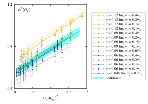
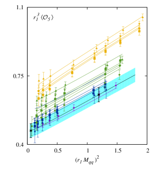
Figure 1: Chiral-continuum extrapolation of the matrix elements $\langle\mathcal{O}_{1}\rangle$ (left panel) and $\langle\mathcal{O}_{5}\rangle$ (right panel) in $r_{1}$ units. The data points are the renormalized matrix elements shown as functions of the valence taste-pion mass-squared for the different lattice spacings and sea quark masses, as indicated in the legend box. The lines indicate the result of the fit, with the black line and cyan band showing the continuum extrapolation.

4 Systematic error budget

The dominant systematic errors in our calculation are due to the chiral-continuum extrapolation, heavy-quark discretization effects, and the perturbative matching of the four-quark operators. In the two former cases, we account for the error due the truncation of the corresponding expansions by considering fits that include more (higher order) terms with Bayesian constrained coefficients until the results (central values and error bars) stabilize. In this way, the statistical fit error includes the systematic error from truncation. This is illustrated in Figure 2 for $\langle\mathcal{O}_{1}\rangle$ and $\langle\mathcal{O}_{5}\rangle$. The stability plots for the other matrix elements are very similar.

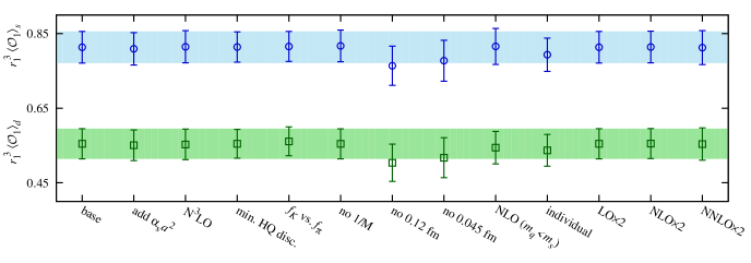
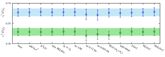
Figure 2: Stability plots for $\langle\mathcal{O}_{1}\rangle$ and $\langle\mathcal{O}_{5}\rangle$ showing the variation of the chiral-continuum fits with different choices for the fit function and parameters. The bands show the result of the preferred fits.

We see that our fits are stable under adding $O(\alpha_{s}a^{2})$ terms, adding N³LO analytic terms, dropping higher-order HQ discretization terms, using $f_{K}$ instead of $f_{\pi}$, dropping the $1/M$ terms from the heavy-meson expansion, excluding data from the coarsest (finest) lattice spacing, and increasing the prior widths.

	$\langle\mathcal{O}_{1}\rangle_{s}$		$\langle\mathcal{O}_{1}\rangle_{d}$		$\langle\mathcal{O}_{i}\rangle_{s}$ ( $i>1$)		$\langle\mathcal{O}_{i}\rangle_{d}$ ($i>1$)
source	2011	2014	2011	2014	2011	2014	2011	2014
comb. stat. $\chi$PT	7	5	15	7	3–11	4–12	4.3–16	6–15
HQ disc.	4	included	4	included	4	included	4	included
inputs	5.1	included	5.1	included	5.1	included	5.1	included
renormalization	8	6.4	8	6.4	8	6.4	8	6.4
finite volume	1	1	1	1	1	1	1	1
total	12	8	18	10	10–15	8–13	11–19	9–17

Table 1: Comparison of the error budgets for $\langle\mathcal{O}_{i}\rangle$ from Ref. [11] (2011) with this analysis (2014). Here, “included” means these errors are now included via Bayesian priors in the combined statistical, $\chi$PT error.

source	2012	2014
combined statistics, $\chi$PT	3.7	1.4
wrong spin	3.2	NA
HQ discretization	0.3	included
inputs	0.7	included
renormalization	0.5	0.5
finite volume	0.5	0.5
total	5	1.6

Table 2: Comparison of the error budgets for $\xi$ from Ref. [5] (2012) with this analysis (2014). Here, “included” means these errors are now included via Bayesian priors in the combined statistical, $\chi$PT error.

There are errors of $O(\alpha_{s}^{2})$ in our calculation since the renormalization coefficients are calculated in perturbation theory at one-loop order. The one-loop coefficients for the $B$-meson mixing operators are $O(1)$, and we therefore estimate the error as the average of $\alpha_{s}^{2}$ from all four lattice spacings. This yields the error shown in Table 1. We are currently investigating the effect of using the mostly nonperturbative renormalization method introduced in Ref. [18] for heavy-light currents. Because the MILC ensembles have large spatial volumes with $M_{\pi}L\gtrsim 3.8$, we expect finite volume errors to be a subdominant source of error, contributing at the 1% level or less. We are currently in the process of including finite volume corrections in the chiral expansion. The estimates shown in Tables 1 and 2 are from our decay constant analysis [19].

5 Conclusions and outlook

We present nearly final systematic error budgets for our analysis of the matrix elements $\langle\mathcal{O}_{i}\rangle$ and $\xi$. Tables 1 and 2 show comparisons of our current error budgets with our previous results. We find significant improvement in all cases. For $\xi$ we expect a final error of $\lesssim 2\%$, more than a factor of two smaller than our previous result. This is only in part due to the fact that Ref. [5] used a much smaller subset of MILC ensembles. Another factor is that with simultaneous fits to all three operators in our present analysis there is no ”wrong spin” error anymore. Once our results are final, we also plan to combine those for the $\langle\mathcal{O}_{i}\rangle$ with the companion analysis of the $B_{s}$ and $B_{d}$ decay constants [20] to obtain results for the corresponding bag parameters.

References

- [1] S. Aoki, et al. [FLAG], Eur. Phys. J. C 74, no. 9, 2890 (2014) [arXiv:1310.8555 [hep-lat]].
- [2] K. A. Olive et al. [Particle Data Group], Chin. Phys. C 38, 090001 (2014).
- [3] E. Gámiz et al. [HPQCD Collaboration], Phys. Rev. D 80, 014503 (2009) [arXiv:0902.1815 [hep-lat]].
- [4] C. Albertus et al. [RBC/UKQCD Collaboration], Phys. Rev. D 82, 014505 (2010) [arXiv:1001.2023 [hep-lat]]; Y. Aoki, T. Ishikawa, T. Izubuchi, C. Lehner and A. Soni, arXiv:1406.6192 [hep-lat].
- [5] A. Bazavov et al. [Fermilab Lattice and MILC Collaborations], Phys. Rev. D 86, 034503 (2012) [arXiv:1205.7013 [hep-lat]].
-
[6]
N. Carrasco et al. [ETM Collaboration],
JHEP 1403, 016 (2014)
[arXiv:1308.1851 [hep-lat]];
PoS LATTICE2013, 382 (2014) [arXiv:1310.1851 [hep-lat]]. - [7] R. J. Dowdall et al. [HPQCD Collaboration], arXiv:1411.6989 [hep-lat].
- [8] A. Bazavov et al., Rev. Mod. Phys. 82, 1349 (2010) [arXiv:0903.3598 [hep-lat]].
- [9] C.C. Chang et al. [Fermilab Lattice and MILC Collaborations], PoS LATTICE2013, 405 (2013) arXiv:1311.6820 [hep-lat].
- [10] A.X. El-Khadra, A.S. Kronfeld and P.B. Mackenzie, Phys. Rev. D 55, 3933 (1997) [hep-lat/9604004].
- [11] C.M. Bouchard et al. [Fermilab Lattice and MILC Collaborations], PoS LATTICE2011, 274 (2011) [arXiv:1112.5642 [hep-lat]].
- [12] E. D. Freeland et al. [Fermilab Lattice and MILC Collaborations], PoS LATTICE2012, 124 (2012) [arXiv:1212.5470 [hep-lat]].
- [13] M. Beneke, G. Buchalla, C. Greub, A. Lenz and U. Nierste, Phys. Lett. B 459, 631 (1999) [hep-ph/9808385].
- [14] A. J. Buras, S. Jäger and J. Urban, Nucl. Phys. B 605, 600 (2001) [hep-ph/0102316].
- [15] J. A. Bailey et al. [Fermilab Lattice and MILC Collaborations], Phys. Rev. D 89, 114504 (2014) [arXiv:1403.0635 [hep-lat]].
- [16] C. Bernard [MILC Collaboration], Phys. Rev. D 87, 114503 (2013) [arXiv:1303.0435 [hep-lat]].
- [17] C. Aubin and C. Bernard, Phys. Rev. D 73, 014515 (2006) [hep-lat/0510088].
- [18] J. Harada, S. Hashimoto, K. I. Ishikawa, A. S. Kronfeld, T. Onogi and N. Yamada, Phys. Rev. D 65, 094513 (2002) [Erratum-ibid. D 71, 019903 (2005)] [hep-lat/0112044].
- [19] A. Bazavov et al. [Fermilab Lattice and MILC Collaborations], Phys. Rev. D 85, 114506 (2012) [arXiv:1112.3051 [hep-lat]].
- [20] E.T. Neil et al. [Fermilab Lattice and MILC collaborations], these proceedings.