Deconfinement transition in SU($2$) Yang-Mills theory: A two-loop study

Abstract

In a recent work we have proposed a perturbative approach for the study of the phase transition of pure Yang-Mills theories at finite temperature. This is based on a simple massive extension of background field methods in the Landau-DeWitt gauge, where the gluon mass term is related to the existence of Gribov ambiguities. We have shown that a one-loop calculation of the background field effective potential describes well the phase structure of the SU($2$) and SU($3$) theories. Here, we present the calculation of the next-to-leading-order contribution in perturbation theory for the SU($2$) case. In particular, we compute the background field effective potential at two-loop order and the corresponding Polyakov loop, a gauge invariant order parameter of the transition, at one-loop order. We show that the two-loop correction brings the critical temperature closer to its actual value as compared to the previous one-loop result. We also compute the thermodynamic pressure as a function of the temperature and show that two-loop contributions play an important role in the vicinity of the phase transition.

I Introduction

The deconfinement transition of hadronic matter into a plasma of quarks and gluons at high temperature is a remarkable phenomenon. It is thought to have played a role in the early Universe and it is the major subject of investigation of ultrarelativistic heavy ion collisions at CERN and at RHIC. Establishing firmly the existence of this transition in QCD and characterizing its properties is a formidable task which has only been possible thanks to more than three decades of dedicated lattice studies Engels:1980ty ; McLerran:1980pk ; Kuti:1980gh ; see Refs. Petreczky:2012rq ; Philipsen:2012nu for recent reviews. Early calculations clearly established the existence of a phase transition in pure SU($N$) Yang-Mills theories, related to the spontaneous breaking of the center ($Z_{N}$) of the gauge group Engels:1981qx ; Boyd:1995zg . The inclusion of dynamical quarks, first with heavy masses and then with physical masses, has been a central issue in the field for years. Only recently have precise calculations of the thermodynamic properties of QCD with physical quark masses been achieved, with the result that the phase transition of the pure gauge theory becomes a crossover in QCD Bazavov:2014pvz ; Borsanyi:2013bia .

Thanks to asymptotic freedom, standard perturbative approaches make sense at high temperatures and an intense activity has been concerned with computing the thermodynamics and transport properties of the quark-gluon plasma by means of (semi)analytical methods Blaizot:1999ip ; Blaizot:2000fc ; Blaizot:2001vr ; Andersen:1999sf ; Andersen:2002ey ; Andersen:2011sf ; Haque:2013sja ; Arnold:2000dr ; Arnold:2003zc . In this regime, infrared divergences call for the resummation of infinite subclasses of perturbative diagrams, the so-called hard thermal loops Braaten:1989mz ; Braaten:1990az ; Braaten:1991gm . Such high temperature approaches reproduce the thermodynamic properties of the deconfined plasma down to a few times the transition temperature Blaizot:1999ip ; Blaizot:2000fc ; Blaizot:2001vr but fail to capture the physics of the phase transition. It is commonly accepted that the low temperature confining phase cannot be described by means of perturbation theory because of the existence of a Landau pole at low energy, where the running coupling diverges.

Existing nonperturbative continuum descriptions of the transition region are based on truncations of Dyson-Schwinger equations (DSE), nonperturbative/functional renormalization-group techniques Marhauser:2008fz ; Braun:2007bx ; Braun:2010cy ; Fister:2013bh ; Epple:2006hv ; Alkofer:2006gz ; Fischer:2009wc ; Fischer:2009gk , the Hamiltonian approach of Reinhardt:2012qe ; Reinhardt:2013iia , or two-particle-irreducible (2PI) inspired approaches Fukushima:2012qa ; Fister:2013bh . These have the advantage over lattice calculations that they can easily be used at finite chemical potential Fischer:2013eca ; Fischer:2014vxa ; Fischer:2011mz ; Fischer:2012vc and/or for computing real-time quantities Mueller:2010ah ; Strauss:2012dg ; Haas:2013hpa . To be trustable in these situations though, they have to be tested against lattice calculations in situations where the latter is well under control. Functional renormalization-group (FRG) methods have been shown to correctly describe the phase structure of pure gauge theories, with transition temperatures in agreement with lattice results Braun:2007bx ; Fister:2013bh . Such approaches also provide nontrivial insight concerning dynamical aspects of the deconfinement transition. For instance, an interesting connection between the confinement of static quarks and the infrared (IR) behavior of gluon and ghost correlators has been pointed out Braun:2007bx ; Fister:2013bh . Of course, neither the DSE nor the FRG can be solved exactly and one’s ability to perform actual calculations relies on several assumptions which, even when these are well motivated, can be difficult to check explicitly. A general criticism that many nonperturbative approaches have to face is that they do not always involve a systematic approximation scheme and it is often difficult to compute corrections to the obtained results. Still, the DSE/FRG provide the most powerful nonperturbative tools—apart from lattice techniques—to investigate the physics of the deconfinement transition directly at the level of the basic degrees of freedom of the theory.

In a series of recent works Tissier_10 ; Tissier_11 ; Serreau:2012cg ; Pelaez:2013cpa ; Serreau:2013ila ; Reinosa:2013twa ; Pelaez:2014mxa ; Reinosa:2014ooa , yet a different route for the study of the infrared dynamics of Yang-Mills fields has been proposed. This is based on simple massive extensions of the standard Faddeev-Popov Lagrangian in the Landau gauge and in the Landau-DeWitt gauge. This is motivated by the observation that perturbative calculations of Yang-Mills correlators in the vacuum Tissier_10 ; Tissier_11 ; Pelaez:2013cpa ; Pelaez:2014mxa and at finite temperature Reinosa:2013twa in the massive extension of the Landau gauge action agree well with lattice data down to deep IR momenta. It is worth emphasizing that, if the typical value of the gauge coupling $g$ required for such comparisons is of a few units, the relevant expansion parameter at zero temperature is $g^{2}N/(16\pi^{2})\lesssim 1$. An important feature of the massive theory is that there exist IR safe renormalization-group trajectories, with no Landau pole Tissier_11 ; Serreau:2012cg . Moreover, it has been argued in Serreau:2012cg that such a massive extension naturally arises as an effective theory for Yang-Mills correlators in a new one-parameter family of Landau gauges which, unlike the standard Faddeev-Popov construction, takes into account the existence of Gribov ambiguities. In this approach, the gluon mass term appears as a gauge-fixing parameter which lifts the degeneracy between Gribov copies.

This has been extended to the Landau-DeWitt gauge in the context of background field methods in Reinosa:2014ooa . There, we have shown that a calculation of the background field potential at first nontrivial (one-loop) order in perturbation theory correctly reproduces the phase structure of SU($N$) theories: one finds a confining phase at low temperature and a transition to a deconfined phase at high temperature which is second order for $N=2$ and first order for $N=3$, with transition temperatures in qualitative agreement with known values from lattice calculations. Our one-loop results are similar to those of the FRG studies of Braun:2007bx and actually corroborate the related findings concerning the relation between the IR behavior of gluon and ghost propagators and the existence of a confining phase at low temperature. Definite advantages of such a perturbative approach are, first, that low-order calculations are technically very simple and, second, that they can be systematically improved by computing higher orders. If at asymptotically high temperatures, the expansion parameter is $g$ due to collective infrared effects which necessitate the resummation of hard thermal loops Blaizot:2001nr , near the transition region and below, the effective gluon mass tames some of the infrared problems of the perturbative series and it is not clear what is the relevant expansion parameter. It is the purpose of the present article to study the importance of such higher-order terms by computing the background field potential, the Polyakov loop and the thermodynamic pressure at next-to-leading order in the perturbative expansion.

Before embarking in actual calculations, let us make some general comments concerning the massive extension of the Faddeev-Popov action in the class of (Landau or Landau-DeWitt) gauges considered here. What usually prevents a mass term in the gauged-fixed action is obviously not gauge invariance, but BRST symmetry. The latter is a property of the Faddeev-Popov action, which is known to be valid at best in the high energy perturbative regime. But the Faddeev-Popov construction is certainly wrong in general since it ignores the existence of Gribov copies and, hence, does not completely fix the gauge. In fact, it is well known that the only truly nonperturbative formulation of the gauge-fixed theory known so far, that is the lattice, cannot accommodate the BRST symmetry without leading to undefined zero over zero ratios Neuberger:1986vv ; Neuberger:1986xz .

A consistent quantization procedure, free of Gribov ambiguities, is likely to break the BRST symmetry. A well-known example is the minimal Landau gauge on the lattice, where one picks up a random Gribov copy on each gauge orbit Cucchieri:2014via . Examples in the continuum include the so-called (refined) Gribov-Zwanziger approach Gribov77 ; Zwanziger89 ; Zwanziger92 ; Vandersickel:2012tz ; Dudal08 or the averaging procedure of Serreau:2012cg , already mentioned. In the latter case, the bare gluon mass originates from the averaging procedure and is simply a gauge-fixing parameter which explicitly breaks the BRST symmetry. Such gauge-fixing procedures provide efficient starting points for perturbative calculations of Yang-Mills correlators and, for the latter, of the phase structure of the theory at finite temperature. In both approaches the BRST breaking is soft and the gauge-fixed actions present modified (non-nilpotent) BRST symmetries, which ensure their renormalizability. At this point, it is worth emphasizing that the continuum approaches mentioned above also introduce, in one way or another, a BRST-breaking ingredient. This typically appears through choices of boundary conditions and/or ultraviolet subtractions in the context of DSE Dudal:2014rxa , or through the infrared regulator in FRG approaches.

The plan of the paper is as follows. Section II sets the scene and briefly recalls the basics of the $Z_{N}$ transition and of static quark confinement. In Sec. III we present the massive extension of the Landau-DeWitt gauge and derive the corresponding Feynman rules. In Sec. IV, we summarize the calculation of the two-loop correction to the background field effective potential and in Sec. V, we give the corresponding expression for the one-loop correction to the Polyakov loop. Finally, in Sec. VI, we present our results concerning the order of the phase transition and the value of the transition temperature as well as the temperature dependence of the Polyakov loop and of the thermodynamic pressure. The essential steps of our calculations are presented in the main text while the technical details are gathered in the Appendixes.

Although we specify to the case $N=2$ throughout this work, some formulas are valid for arbitrary $N$. An important observation is that many steps of our calculations are similar to those in the massive extension of the Landau gauge, i.e., at vanishing background field. In fact, when expressed in an appropriate color basis, the Feynman rules of the theory have the same form as those in the Landau gauge, with the only difference that the momenta get shifted by an amount proportional to the background field. The key point is that, because of the residual global color symmetry, these shifts are conserved at the interaction vertices. This allows us to use various simplifying manipulations, detailed in Appendix A, and to reduce all the two-loop diagrams contributing to the background field potential to simple scalarlike sum-integrals; see Appendix B. The evaluation of the corresponding Matsubara sums is presented in Appendix C, which allows us to write the background field potential in a rather simple form in Appendix D. In Appendix E, we detail the calculation of the Polyakov loop at one-loop order in the presence of the nontrivial background field. In particular, this demonstrates explicitly that the Polyakov loop vanishes if and only if the minimum of the background field potential takes particular, $Z_{2}$–symmetric values. This confirms, at this order of approximation, that the background field itself can be used as an order parameter for confinement, as advocated in Braun:2007bx ; Braun:2010cy ; Fister:2013bh . Finally, we provide, in Appendix F, a general proof that the Polyakov loop vanishes when the background field takes $Z_{2}$–symmetric values. We do not have a similar proof for the converse.

II Confinement-deconfinement transition in Yang-Mills theory

We consider the Euclidean Yang-Mills action in $d=4-2\epsilon$ dimensions

$$S_{\rm YM}[A]=\frac{1}{2}\int_{x}\hbox{tr}\left\{F_{\mu\nu}F_{\mu\nu}\right\}\,,$$ (1)

where $F_{\mu\nu}=\partial_{\mu}A_{\nu}-\partial_{\nu}A_{\mu}-ig_{0}[A_{\mu},A_{\nu}]$, with $g_{0}$ the bare coupling constant and $A$ the bare gauge field, $iA$ being an element of the Lie algebra of SU($N$). We have also defined $\int_{x}\equiv\int_{0}^{\beta}d\tau\int d^{d-1}x$, with $\beta=1/T$ the inverse temperature.

Let us recall some basic aspects of the deconfinement transition to be considered below. The free energy $F_{q}$ of an isolated static quark in a thermal gluon bath is directly related to the expectation value of the traced Polyakov loop—which we refer to as the Polyakov loop for short in what follows—as Svetitsky:1985ye

$$e^{-\beta(F_{q}-F_{0})}=\frac{1}{N}\hbox{tr}\left<P\exp\left\{ig_{0}\int_{0}^{\beta}\!\!d\tau A_{0}(\tau,{\bf x})\right\}\right>\equiv\ell,$$ (2)

where $F_{0}$ is the free energy in the absence of quark. Here, $P$ orders the matrix fields $A_{0}(\tau,{\bf x})$ from left to right with decreasing value of their time arguments and the brackets refer to the average in the theory defined by the action (1). A vanishing $\ell$ signals an infinite free energy, hence a quark confining phase, while $\ell\neq 0$ is interpreted as a phase where isolated static quarks are energetically allowed.

It is well known Svetitsky:1985ye that the Polyakov loop gets multiplied by a phase under generalized gauge transformations that leave the Yang-Mills action at finite temperature invariant and which are $\beta$ periodic in imaginary time, up to an element of the center of the group. This means that the deconfined phase is necessarily a phase where this symmetry group, or more precisely the quotient of the group of generalized gauge transformations by the subgroup of standard gauge transformations—which is isomorphic to $Z_{N}$—is spontaneously broken. Note that the converse is not necessarily true: Although this is not the expected behavior, one could, in principle, imagine a situation where the center is spontaneously broken but where the Polyakov loop still vanishes, the breaking being only manifest at the level of higher-order correlations. This emphasizes the fact that the confined or deconfined nature of the system, in the sense described above, is not the breaking of the $Z_{N}$ symmetry itself but really the zero or nonzero value of the Polyakov loop (or of any equivalent order parameter). In what follows, we shall compute the Polyakov loop at one-loop order within the massive extension of the Landau-DeWitt gauge put forward in Reinosa:2014ooa .

III The massive Landau-DeWitt action

III.1 General setup

We quantize the theory using the background field method DeWitt:1967ub ; Abbott:1980hw ; Abbott:1981ke ; Weinberg:1996kr , where we introduce an a priori arbitrary background field configuration $\bar{A}_{\mu}$ and define the fluctuating field $a_{\mu}=A_{\mu}-\bar{A}_{\mu}$. The Landau-DeWitt gauge condition reads

$$\bar{D}_{\mu}a_{\mu}=0,$$ (3)

where $\bar{D}_{\mu}\varphi=\partial_{\mu}\varphi-ig_{0}[\bar{A}_{\mu},\varphi]$ for any field $i\varphi$ in the Lie algebra of the gauge group. Our gauge-fixed action reads Reinosa:2014ooa

$$S=\!\int_{x}\hbox{tr}\left\{{1\over 2}F_{\mu\nu}F_{\mu\nu}+{m_{0}^{2}}a_{\mu}a_{\mu}+2\bar{D}_{\mu}\bar{c}D_{\mu}c+2ih\bar{D}_{\mu}a_{\mu}\right\}\!,$$ (4)

with $h$ a (real) Nakanishi-Lautrup field and $c$ and $\bar{c}$ the Faddeev-Popov ghosts and antighost fields. In terms of the field $a_{\mu}$, we have

$$F_{\mu\nu} =\bar{F}_{\mu\nu}+\bar{D}_{\mu}a_{\nu}-\bar{D}_{\nu}a_{\mu}-ig_{0}[a_{\mu},a_{\nu}],$$ (5)

with $\bar{F}_{\mu\nu}^{a}=F_{\mu\nu}^{a}[\bar{A}]$ the field strength tensor evaluated at $A=\bar{A}$, and

$$D_{\mu}\varphi=\partial_{\mu}\varphi-ig_{0}[A_{\mu},\varphi]=\bar{D}_{\mu}\varphi-ig_{0}[a_{\mu},\varphi].$$ (6)

The action (4) has the obvious property

$$S[\bar{A},\varphi]=S[\bar{A}^{U},U\varphi U^{-1}],$$ (7)

where $\varphi=(a,c,\bar{c},h)$, $U$ is a local SU($N$) matrix, and

$$\bar{A}_{\mu}^{U}=U\bar{A}_{\mu}U^{-1}+\frac{i}{g_{0}}U\partial_{\mu}U^{-1}.$$ (8)

At the level of the (quantum) effective action $\Gamma$ this implies Weinberg:1996kr

$$\Gamma[\bar{A},\varphi]=\Gamma[\bar{A}^{U},U\varphi U^{-1}],$$ (9)

where the fields $\varphi$ are now to be understood as average values in the presence of sources.

In principle, to evaluate physical observables at zero sources, one should minimize $\Gamma[\bar{A},\varphi]$ with respect to $\varphi$ at a given $\bar{A}$. It can be argued, however, that one can alternatively minimize the functional

$$\tilde{\Gamma}[\bar{A}]=\Gamma[\bar{A},0]$$ (10)

with respect to the background field $\bar{A}$ Braun:2007bx ; Fister:2013bh ; Reinosa:2014ooa . This functional obeys the background gauge symmetry

$$\tilde{\Gamma}[\bar{A}]=\tilde{\Gamma}[\bar{A}^{U}],$$ (11)

which is trivially preserved in perturbation theory. The Polyakov loop can be obtained as

$$\ell(T)=\frac{1}{N}\hbox{tr}\left<P\exp\left\{ig_{0}\int_{0}^{\beta}\!\!d\tau(\bar{A}_{0}+a_{0})(x)\right\}\right>_{\rm min},$$ (12)

with $x\equiv(\tau,{\bf x})$ and where the brackets stand for an average in the gauge-fixed theory (4). The right-hand side of Eq. (12) is evaluated at an absolute minimum $\bar{A}(x)=\bar{A}_{\rm min}(x)$ of $\tilde{\Gamma}[\bar{A}]$. Because the Polyakov loop involves only the temporal component of the background field and because $\bar{A}_{\rm min}(x)=\langle A(x)\rangle_{\rm min}$ (since $\langle a(x)\rangle_{\rm min}=0$ by construction) is $x$ independent, it is sufficient to consider homogeneous background fields in the temporal direction $\bar{A}_{\mu}(x)=\bar{A}_{0}\delta_{\mu 0}$. Moreover, the Hermitian matrix $\bar{A}_{0}$ can be diagonalized by means of a global SU($N$) rotation and one can thus, with no loss of generality, restrict $\bar{A}_{0}$ to the Cartan subalgebra of the color group. We shall write $\bar{A}_{0}=\bar{A}_{0}^{k}t^{k}$, where $t^{k}$ are the SU($N$) generators in the Cartan subalgebra. We thus have to minimize the background field effective potential

$$V(T,r^{k})=\frac{\tilde{\Gamma}[\bar{A}]}{\beta\Omega}-V_{\rm vac},$$ (13)

where $r^{k}=g_{0}\beta\bar{A}_{0}^{k}$ and $\Omega$ is the spatial volume. We have subtracted $V_{\rm vac}$, the value of the potential at zero temperature which is independent of $r^{\kappa}$, as we shall see below. Finally, the thermodynamic pressure is simply given by

$$p(T)=-V(T,r_{\rm min}^{k}(T))\,,$$ (14)

where $r_{\rm min}^{k}(T)=g_{0}\beta\bar{A}^{k}_{0,{\rm min}}(T)$.

The symmetry (11) implies that the potential (13) is invariant under gauge transformations of the form

$$U(\tau,{\bf x})=\exp\{i\tau\varphi/\beta\},$$ (15)

where $\varphi$ is such that $U^{-1}(0,{\bf x})U(\beta,{\bf x})\propto\mathds{1}$. This implies that the potential is periodic along certain directions in the Cartan subalgebra. Together with the invariance under global color rotations and charge conjugation, this implies that some of the extrema of the potential have specific locations Reinosa:2014ooa . In the SU($2$) case, these considerations show that the potential is $2\pi$–periodic in $r$ and has extremas at $r=0\,({\rm mod}\,\pi)$. In Appendix F, we provide a general proof that, among those, the values $r=\pi\,({\rm mod}\,2\pi)$ are such that $\ell=0$ and thus correspond to a confined phase. This supports the general expectation Braun:2007bx ; Braun:2010cy ; Fister:2013bh that the background field itself can be used as an order parameter. Our proof is, however, not complete because the converse, i.e., $\ell=0\Rightarrow r=\pi({\rm mod}\,2\pi)$, is missing. In the present work, we shall, however, explicitly show that the equivalence holds at next-to-leading order in the loop expansion.

III.2 Renormalization

We introduce renormalized parameters and fields, related to the corresponding bare quantities in the usual way:

$$m_{0}^{2}=Z_{m^{2}}m^{2}\,,\quad g_{0}=Z_{g}g\,,$$ (16)

and

$${\bar{A}}$$ ,

,

(17)

where we have kept the same notation for bare (left) and renormalized (right) fields for simplicity. Notice that the background field $\bar{A}$ and the fluctuating field $a$ have different renormalization factors Binosi:2013cea . The background field gauge symmetry (9) implies that the product $g_{0}\bar{A}$ is finite Weinberg:1996kr . In the following we impose the renormalization condition

$$Z_{g}\sqrt{Z_{\bar{A}}}=1$$ (18)

for the finite parts as well, so that $g_{0}\bar{A}\to g\bar{A}$. From here on, we only consider renormalized quantities unless explicitly stated. The values of the parameters $m$ and $g$ must be fixed from some external input, e.g., lattice data.

To set the value of the renormalized mass $m$, one would ideally use the value of a physical observable such as a glueball mass. An easier possibility in practice is to fix this parameter by employing lattice results for gauge-dependent quantities such as the the Yang-Mills correlators. In principle, this requires lattice results in the same gauge as described above, involving an average of Gribov copies. Instead, existing gauge-fixed lattice calculations typically select a particular Gribov copy in the so-called first Gribov region, where the Faddeev-Popov operator is positive definite. Still, explicit calculations in the massive extension of the Faddeev-Popov Lagrangian in the Landau gauge show that there exists a value of the renormalized mass which allows one to quantitatively reproduce the lattice data for the Yang-Mills correlators at vanishing temperature Reinosa:2013twa .

No lattice calculation exists so far in the Landau-DeWitt gauge with homogeneous temporal background field as considered here. However, at zero temperature the background field vanishes and the latter reduces to the standard Landau gauge. In the present work, we shall thus use the values of $m$ and $g$ inferred from lattice calculations in the Landau gauge at vanishing temperature. To be consistent with the approximation order considered here, we need the one-loop expressions of the vacuum propagators. These have been computed in Tissier_11 . Using the renormalization conditions

$$\Sigma_{\rm vac}(K^{2}=\mu^{2})=\Pi_{\rm vac}(K^{2}=0)=\Pi_{\rm vac}(K^{2}=\mu^{2})=0,$$ (19)

where $\Sigma_{\rm vac}(K^{2})$ and $\Pi_{\rm vac}(K^{2})$ denote, respectively, the renormalized ghost and transverse gluon self-energies in the vacuum, the best fits to lattice data give $m\simeq 680$ MeV and $g\simeq 7.5$, with $\mu=1$ GeV for SU($2$) in $d=4$.

III.3 Feynman rules

For the homogeneous background fields considered here, $\bar{A}_{\mu}(x)=\bar{A}_{0}\delta_{\mu 0}$, the curvature term vanishes: $\bar{F}_{\mu\nu}=0$. Moreover, as emphasized above, the background field $\bar{A}_{0}$ can be taken in the Cartan subalgebra of the gauge group. For SU($2$), the latter has only one direction which we choose along the third axis in color space. It is convenient to work with the basis of generators

$$t^{0}=t^{3}\,,\quad t^{\pm}=\frac{t^{1}\pm it^{2}}{\sqrt{2}},$$ (20)

which satisfy

$$[t^{\kappa},t^{\lambda}]=\varepsilon^{\kappa\lambda\tau}t^{-\tau}\,,\quad\hbox{tr}\{t^{\kappa}t^{-\lambda}\}=\frac{\delta^{\kappa\lambda}}{2}$$ (21)

where $\varepsilon^{\kappa\lambda\tau}$ is the completely antisymmetric tensor, with $\varepsilon^{0+-}=1$. We denote any element of the gauge group Lie algebra as $\varphi=\varphi^{\kappa}t^{\kappa}$. The components of the background covariant derivative are

$$\left(\bar{D}_{\mu}\varphi\right)^{\kappa}=\left(\partial_{\mu}-i\kappa g\bar{A}_{\mu}^{3}\right)\varphi^{\kappa}\to-iK_{\mu}^{\kappa}\,\tilde{\varphi}^{\kappa}(K),$$ (22)

where our convention for the Fourier transform is

$$\tilde{\varphi}(K)=\int_{x}e^{iK\cdot x}\varphi(x),$$ (23)

such that $\partial_{\mu}\to-iK_{\mu}$. Here, we defined the shifted momentum

$$K_{\mu}^{\kappa}=K_{\mu}+\kappa g\bar{A}^{3}_{\mu},$$ (24)

which satisfies

$$(-K)_{\mu}^{-\kappa}=-K_{\mu}^{\kappa}.$$ (25)

Figure 1: Diagrammatic representation of the ghost (dashed) and gluon (curly) propagators for momentum $K$ and color charge $\kappa$. The orientation of the flow of momentum and color charge is arbitrary.

The background field breaks the global color group but there remains a residual symmetry under those color rotations that leave it invariant. In the SU($2$) theory, this is the group of SO($2$) $\sim$ U($1$) transformations, under which $\varphi^{0}\to\varphi^{0}$ and $\varphi^{\pm}\to e^{\pm i\alpha}\varphi^{\pm}$, with $\alpha$ a constant phase. Accordingly, we refer to $\varphi^{0}$ as the “neutral” component and to $\varphi^{\pm}$ as the “charged” components. The (temporal) background field plays the role of an external Abelian field coupled to the charged components, which leads to a simple shift of momentum $\pm g\bar{A}_{\mu}^{3}$. Equivalently, it can be seen as an imaginary chemical potential associated with the conserved U($1$) charge. The residual color symmetry guarantees that the corresponding charge is conserved upon propagation and at the interaction vertices.

It is an easy exercise to compute the Feynman rules of the theory in the basis (20). To each propagator and to each leg of an interaction vertex is associated a flow of color charge, which we define to follow the flow of momentum. The tree-level ghost and gluon propagators for momentum $K$ and charge state $\kappa$, represented in Fig. 1, are given by

$$\langle c^{-\kappa}(-K){\bar{c}}^{\,\kappa}(K)\rangle \equiv G^{\kappa}(K)=G_{0}(K^{\kappa}),$$ (26)

$$\langle a_{\mu}^{-\kappa}(-K)a_{\nu}^{\kappa}(K)\rangle \equiv G_{\mu\nu}^{\kappa}(K)={\cal P}_{\mu\nu}(K^{\kappa})G_{m}(K^{\kappa}),$$ (27)

where we denote the scalar propagator of mass $\alpha$ by

$$G_{\alpha}(K)\equiv\frac{1}{K^{2}+\alpha^{2}}\,,$$ (28)

and where $\smash{{\cal P}_{\mu\nu}^{\perp}(K)\equiv\delta_{\mu\nu}-K_{\mu}K_{\nu}/K^{2}}$. Note the identities $G^{\kappa}(K)=G^{-\kappa}(-K)$ and $G^{\kappa}_{\mu\nu}(K)=G^{-\kappa}_{\mu\nu}(-K)$, which follow from (25) and which simply reflect the fact that the choice of orientation of the momentum/charge flow in the diagrams of Fig. 1 is arbitrary.

Figure 2: Diagrammatic representation of the cubic derivative vertices. The momenta and color charges are either all outgoing or all incoming.

Figure 3: Diagrammatic representation of the four-gluon vertex. All momenta and color charges are either all outgoing or all incoming.

The cubic (derivative) vertices are represented on Fig. 2, with the convention that all momenta and color charges are outgoing. The ghost-antighost-gluon vertex is given by

$$g\varepsilon^{\kappa\lambda\tau}K_{\nu}^{\kappa},$$ (29)

and the three-gluon vertex reads

$$\frac{g}{6}\varepsilon^{\kappa\lambda\tau}\Big{[}\delta_{\mu\rho}\left(K^{\kappa}_{\nu}-Q^{\tau}_{\nu}\right)\!+\!\delta_{\nu\mu}\left(L^{\lambda}_{\rho}-K^{\kappa}_{\rho}\right)\!+\!\delta_{\rho\nu}\left(Q^{\tau}_{\mu}-L^{\lambda}_{\mu}\right)\!\Big{]},$$ (30)

where the various momenta, color charges, and spacetime indices are organized as in Fig. 2. The structure constant $\varepsilon^{\kappa\lambda\tau}$ guarantees that the charge is conserved at the vertex: $\kappa+\lambda+\tau=0$. Finally, the four-gluon vertex is

$$\frac{g^{2}}{24}\sum_{\omega}\Big{[}\, \varepsilon^{\kappa\lambda\omega}\varepsilon^{-\omega\tau\xi}(\delta_{\mu\rho}\delta_{\nu\sigma}-\delta_{\mu\sigma}\delta_{\nu\rho})$$

$$+ \varepsilon^{\kappa\tau\omega}\varepsilon^{-\omega\lambda\xi}(\delta_{\mu\nu}\delta_{\rho\sigma}-\delta_{\mu\sigma}\delta_{\nu\rho})$$

$$+ \varepsilon^{\kappa\xi\omega}\varepsilon^{-\omega\tau\lambda}(\delta_{\mu\rho}\delta_{\nu\sigma}-\delta_{\mu\nu}\delta_{\rho\sigma})\,\Big{]},$$ (31)

where color charge and spacetime indices are organized as in Fig. 3. Again, the combinations of the group structure constants guarantee that the color charge is conserved: $\kappa+\lambda+\tau+\xi=0$.

Written in the basis (20), the Feynman rules (26)–(31) in the presence of the background field are very similar to the standard ones, usually written in the Cartesian color basis. The essential difference stems in the different structure constants, which can be traced back to the commutation relations (20), and the role of the background field is simply to replace all momenta by shifted ones according to the corresponding color charges. As we shall discuss in a future work, these remarks generalize to any group SU($N$)—in fact to any compact Lie group with a semisimple Lie algebra. For $N=2$, one has the identities

$$\varepsilon^{(-\kappa)(-\lambda)(-\tau)}=-\varepsilon^{\kappa\lambda\tau}$$ (32)

and

$$\sum_{\omega}\varepsilon^{\kappa\lambda\omega}\varepsilon^{-\omega\tau\xi}=\delta^{\kappa,-\xi}\delta^{\lambda,-\tau}-\delta^{\kappa,-\tau}\delta^{\lambda,-\xi}.$$ (33)

Using (25) and (32), one checks that the vertices (29)–(31) are unchanged if all momenta and color charges are incoming.

IV The background field potential at ${\cal O}(g^{2})$

We consider the loop expansion of the background field potential, which corresponds to a perturbative expansion in powers of the renormalized coupling $g$ with $g\bar{A}_{0}\sim{\cal O}(1)$. We write the corresponding series as

$$V(T,r)=\sum_{n\geq 0}V^{(n)}(T,r)\,,$$ (34)

with $\smash{V^{(n)}\sim{\cal O}(g^{2n-2})}$ the $n$-loop order contribution. The classical action (4) evaluated at $c=\bar{c}=0$, $a_{\mu}=0$, and $\bar{A}_{\mu}(x)=\bar{A}_{0}\delta_{\mu 0}$ vanishes identically since $\bar{F}_{\mu\nu}=0$. The tree-level contribution to the term $V_{\rm vac}$ in (13) is thus trivially independent of the background field and the tree-level potential is trivial

$$V^{(0)}(T,r)=0\,.$$ (35)

The one-loop contribution has been obtained in Reinosa:2014ooa and the relevant two-loop diagrams are shown in Fig. 4.

Figure 4: Two-loop diagrams contributing to the background field potential.

IV.1 The one-loop contribution

We briefly recall the result of Reinosa:2014ooa . Introducing the function

$${\cal F}_{m}(T,r)=\frac{T}{\pi^{2}} \int_{0}^{\infty}\!\!dq\,q^{2}\Big{\{}\ln\left(1-e^{-\beta\varepsilon_{q}}\right)$$

$$+\ln\left(1+e^{-2\beta\varepsilon_{q}}-2e^{-\beta\varepsilon_{q}}\cos r\right)\Big{\}},$$ (36)

which is such that, for $r\in[0,2\pi]$,

$${\cal F}_{0}(T,r)=\frac{T^{4}}{6}\left[\frac{(r-\pi)^{4}}{2\pi^{2}}-(r-\pi)^{2}+\frac{\pi^{2}}{10}\right],\\$$

the one-loop background field potential can be written as

$$V^{(1)}(T,r)=\frac{3}{2}{\cal F}_{m}(T,r)-\frac{1}{2}{\cal F}_{0}(T,r),$$ (37)

where the first term on the right-hand side is the contribution from the massive gluons and the second one is due to the massless ghosts. It reduces to the well-known Weiss potential Weiss:1980rj ; Gross:1980br in the high temperature limit :

$$V^{(1)}_{T\gg m}(T,r)\approx{\cal F}_{0}(T,r),$$ (38)

whereas it gives a confining, inverted Weiss potential at low temperature, where the contribution from massive modes is suppressed Braun:2007bx ; Fister:2013bh :

$$V^{(1)}_{T\ll m}(T,r)\approx-\frac{1}{2}{\cal F}_{0}(T,r).$$ (39)

IV.2 Two-loop diagrams

Let us start with the ghost-gluon sunset diagram (second diagram of Fig. 4). A straightforward application of the Feynman rules derived above yields

$$V^{(2)}_{\rm 1g2gh}=\sum_{\kappa,\lambda,\tau}{\cal C}_{\kappa\lambda\tau}\Big{[}- \frac{g^{2}}{2}\int_{Q,K}Q_{\mu}^{\kappa}{\cal P}^{\perp}_{\mu\nu}(L_{\tau})K_{\nu}^{\lambda}$$

$$\times G_{0}(Q_{\kappa})G_{0}(K_{\lambda})G_{m}(L_{\tau})\Big{]},$$ (40)

with $Q+K+L=0$ and $\kappa+\lambda+\tau=0$. We employ the general notations $Q_{\mu}\equiv(\omega_{n},\bf q\,)$, with $\omega_{n}=2\pi nT$, and

$$\int_{Q}\equiv\mu^{2\epsilon}\,T\sum_{n\in\mathds{Z}}\int\frac{d^{d-1}q}{(2\pi)^{d-1}}\equiv\mu^{2\epsilon}\,T\sum_{n\in\mathds{Z}}\int_{\bf q},$$ (41)

with $\mu$ an arbitrary mass scale and we recall that $d=4-2\epsilon$. We have also introduced the completely symmetric tensor

$${\cal C}_{\kappa\lambda\tau}=\left(\varepsilon_{\kappa\lambda\tau}\right)^{2},$$ (42)

whose components vanish unless $\kappa+\lambda+\tau=0$ and are equal to one otherwise. It follows from Eqs. (32) and (33) that

$$\sum_{\tau}{\cal C}_{\kappa\lambda\tau}=1-\delta_{\kappa\lambda},$$ (43)

which imply ($N=2$)

$$\sum_{\lambda\tau}{\cal C}_{\kappa\lambda\tau}=N\quad{\rm and}\quad\sum_{\kappa\lambda\tau}{\cal C}_{\kappa\lambda\tau}=N(N^{2}-1)\,.$$ (44)

For a vanishing background field, the term within brackets in the right-hand side of Eq. (IV.2) is nothing but the expression of the ghost-gluon sunset in the massive extension of the Landau gauge, up to the corresponding color factor $N(N^{2}-1)=6$. The latter is recovered using (44). The expression (IV.2) illustrates that the two-loop perturbative diagram at nonvanishing background can be obtained from the corresponding one at $\bar{A}=0$ as follows: First, one writes the momentum integrals in the massive Landau gauge in terms of three momenta $Q$, $K$, and $L$, up to the color factor $N(N^{2}-1)$; then, one shifts the momenta to $Q_{\kappa}$, $K_{\lambda}$, and $L_{\tau}$ and averages with the weight ${\cal C}_{\kappa\lambda\tau}$. This property can be anticipated from the Feynman rules described above and actually generalizes to any closed diagram, with an appropriate weight factor. The conservation of color charge at the interaction vertices implies the conservation of the shifted momenta under the loop integrals, e.g., $Q_{\kappa}+K_{\lambda}+L_{\tau}=0$ in the two-loop case above. This leads to important simplifications of the calculations in the Landau-DeWitt gauge, as detailed in the Appendixes. Let us finally mention that the expression (IV.2) and the above remarks actually generalize to SU($N$), where the tensor (42) involves the appropriate structure constant. If Eq. (43) is specific to the case $N=2$, the properties (44) are true for arbitrary $N$.

For later use, we rewrite Eq. (IV.2) in a more compact form. Using the conservation of shifted momenta under the sum in (IV.2), we have

$$-Q_{\mu}^{\kappa}{\cal P}_{\mu\nu}^{\perp}(L_{\tau})K_{\nu}^{\lambda}=\frac{Q^{2}_{\kappa}K^{2}_{\lambda}-(Q_{\mu}^{\kappa}K_{\mu}^{\lambda})^{2}}{L_{\tau}^{2}}.$$ (45)

Furthermore, writing

$$\frac{G_{m}(L)}{L^{2}}=\frac{1}{m^{2}}\left[G_{0}(L)-G_{m}(L)\right],$$ (46)

we obtain

$${V^{(2)}_{\rm 1g2gh}=\frac{g^{2}}{2m^{2}}\sum_{\kappa,\lambda,\tau}{\cal C}_{\kappa\lambda\tau}\Big{[}I^{\kappa\lambda\tau}_{000}-I^{\kappa\lambda\tau}_{00m}\Big{]},}$$ (47)

in terms of the two-loop integral

$${I^{\kappa\lambda\tau}_{\alpha\beta\gamma}\equiv\int_{Q,K}\!\!\big{[}Q^{2}_{\kappa}K_{\lambda}^{2}-(Q_{\mu}^{\kappa}K_{\mu}^{\lambda})^{2}\big{]}G_{\alpha}(Q_{\kappa})G_{\beta}(K_{\lambda})G_{\gamma}(L_{\tau}),}$$ (48)

which is needed only for the case $\kappa+\lambda+\tau=0$. In Appendix B, we rewrite these integrals in terms of simpler scalarlike loop integrals; see Eq. (60) below. Here, we simply notice for later use that $I^{\kappa\lambda\tau}_{\alpha\beta\gamma}$ is invariant under the simultaneous permutation of the upper and lower indices, when the corresponding shifts of momenta add up to zero:

$$I^{\kappa\lambda\tau}_{\alpha\beta\gamma}=I^{\kappa\tau\lambda}_{\alpha\gamma\beta}=\ldots\quad{\rm for}\quad\kappa+\lambda+\tau=0.$$ (49)

The two diagrams with purely gluonic loops can be treated in a similar way. We give more details in Appendix  A and simply state the results here. The double tadpole diagram (first diagram of Fig. 4) yields

$${V^{(2)}_{\rm 2g}=\frac{g^{2}}{4}\sum_{\kappa,\lambda,\tau}{\cal C}_{\kappa\lambda\tau}\left[(d^{2}-3d+3)J_{m}^{\kappa}J_{m}^{\lambda}-J^{\kappa}_{\mu\nu}J^{\lambda}_{\mu\nu}\right],}$$ (50)

where we have defined the tadpole integrals

$$J_{\alpha}^{\kappa}\equiv\int_{Q}G_{\alpha}(Q_{\kappa})$$ (51)

and

$$J_{\mu\nu}^{\kappa}\equiv\int_{Q}\frac{Q^{\kappa}_{\mu}Q^{\kappa}_{\nu}}{Q^{2}_{\kappa}}G_{m}(Q_{\kappa}).$$ (52)

As for the gluon sunset diagram (third diagram of Fig. 4), we obtain

$$V^{(2)}_{\rm 3g} =-\frac{g^{2}}{4}\sum_{\kappa,\lambda,\tau}{\cal C}_{\kappa\lambda\tau}\Bigg{\{}J_{m}^{\kappa}J_{m}^{\lambda}-J^{\kappa}_{\mu\nu}J^{\lambda}_{\mu\nu}$$

$$-\frac{4}{m^{2}}\left[\left(d-\frac{5}{4}\right)I^{\kappa\lambda\tau}_{mmm}-(d-1)I^{\kappa\lambda\tau}_{mm0}+\frac{1}{4}I^{\kappa\lambda\tau}_{m00}\right]\Bigg{\}},$$

where (49) has been used.

IV.3 Counterterm contribution

The expressions derived in the previous section contain ultraviolet (UV) divergences. These are canceled by the counterterms from the original action, as we show explicitly in Appendix D. Here, we compute the relevant counterterm contributions to the background field potential.

Writing the renormalization factors as $Z_{i}=1+\delta Z_{i}$, $i=m^{2},g,a,c$, the counterterm action reads

$$\delta S=\int_{x}\hbox{tr}\Big{\{} \!-\delta Z_{a}\,a_{\mu}(\delta_{\mu\nu}\bar{D}^{2}-\bar{D}_{\mu}\bar{D}_{\nu})a_{\nu}+\delta m^{2}a_{\mu}a_{\mu}$$

$$\!-2\delta Z_{c}\,\bar{c}\,\bar{D}^{2}c+2ih\bar{D}_{\mu}a_{\mu}\Big{\}}+\ldots$$ (54)

where $\delta m^{2}=m^{2}(\delta Z_{m^{2}}+\delta Z_{a})$ and the dots denote terms involving the coupling counterterm $\delta g$, which are not needed in the present work.

Using (22), we obtain, for the ghost counterterm loop,

$$V^{(2)}_{\delta Z_{c}}=-\delta Z_{c}\sum_{\kappa}\int_{Q}Q^{2}_{\kappa}G_{0}(Q_{\kappa})=0\,,$$ (55)

where the last integral vanishes in dimensional regularization. The gluon counterterm loop reads

$$V^{(2)}_{\delta Z_{A},\delta m^{2}} =\frac{1}{2}\sum_{\kappa}\int_{Q}\Big{(}\delta Z_{a}Q^{2}_{\kappa}+\delta m^{2}\Big{)}G^{\kappa}_{\mu\mu}(Q)$$

$$=\frac{d-1}{2}\sum_{\kappa}\int_{Q}\Big{(}\delta Z_{a}Q^{2}_{\kappa}+\delta m^{2}\Big{)}G_{m}(Q_{\kappa})\,.$$ (56)

Then, up to an integral which vanishes in dimensional regularization, the total counterterm contribution can be written in terms of the tadpole integral (51) as

$$V^{(2)}_{\rm ct}=\frac{d-1}{2}m^{2}\delta Z_{m^{2}}\sum_{\kappa}J_{m}^{\kappa}\,.$$ (57)

IV.4 The two-loop contribution

Adding together the various two-loop pieces, we obtain [notice that the contributions from the integral (52) cancel]

$$V^{(2)}=\frac{d-1}{2}m^{2}\delta Z_{m^{2}}\sum_{\kappa}J_{m}^{\kappa}$$

$$\qquad+g^{2}\sum_{\kappa,\lambda,\tau}{\cal C}_{\kappa\lambda\tau}\left\{\frac{(d-1)(d-2)}{4}J_{m}^{\kappa}J_{m}^{\lambda}+\frac{1}{2m^{2}}I^{\kappa\lambda\tau}_{000}\right.$$

$$\qquad+\left.\frac{1}{m^{2}}\left[\left(d-\frac{5}{4}\right)I^{\kappa\lambda\tau}_{mmm}-(d-1)I^{\kappa\lambda\tau}_{mm0}-\frac{1}{4}I^{\kappa\lambda\tau}_{m00}\right]\right\}.$$ (58)

For a vanishing background field, Eq. (58) is nothing but the two-loop free energy density computed in the massive extension of the Landau gauge. As detailed in Appendix B, the integral (48) can be expressed in terms of the tadpole integrals (51) and

$$\tilde{J}_{\alpha}^{\kappa}\equiv\int_{Q}Q_{\kappa}^{0}G_{\alpha}(Q_{\kappa}),$$ (59)

and of the scalar sunset

$$S^{\kappa\lambda\tau}_{\alpha\beta\gamma}\equiv\int_{Q,K}G_{\alpha}(Q_{\kappa})G_{\beta}(K_{\lambda})G_{\gamma}(L_{\tau})\,.$$ (60)

Using Eqs. (91)–(94), our final expression for the two-loop contribution to the background field potential is

$${V^{(2)}} ={\frac{d-1}{2}m^{2}\delta Z_{m^{2}}\sum_{\kappa}J_{m}^{\kappa}}+g^{2}{\sum_{\kappa,\lambda,\tau}{\cal C}_{\kappa\lambda\tau}\Bigg{\{}\frac{1}{4}\left(d^{2}-4d+\frac{15}{4}\right)J_{m}^{\kappa}J_{m}^{\lambda}+\frac{1}{8}J_{0}^{\kappa}J_{m}^{\lambda}-\frac{1}{16}J_{0}^{\kappa}J_{0}^{\lambda}}$$

$$-\frac{1}{m^{2}}\left(d-\frac{11}{8}\right)\tilde{J}_{m}^{\kappa}\tilde{J}_{m}^{\lambda}+\frac{1}{m^{2}}\left(d-\frac{3}{4}\right)\tilde{J}_{0}^{\kappa}\tilde{J}_{m}^{\lambda}-\frac{5}{8m^{2}}\tilde{J}_{0}^{\kappa}\tilde{J}_{0}^{\lambda}+\frac{3m^{2}}{4}\left(d-\frac{5}{4}\right)S_{mmm}^{\kappa\lambda\tau}+\frac{m^{2}}{16}S^{\kappa\lambda\tau}_{m00}\Bigg{\}}\,.$$ (61)

The calculation of the various Matsubara sums and momentum integrals involved in this expression is detailed in Appendix  C. Moreover, we show in Appendix D that it is UV finite (up to an overall, temperature- and background-independent divergence) once the counterterm $\delta Z_{m^{2}}$ has been fixed from the renormalization conditions (19). We also reduce this expression to a sum of one- and two-dimensional (radial) momentum integrals involving thermal, Bose-Einstein distribution functions in the presence of the background field. Our final result for the thermal part (the only one that depends on the background) of the two-loop contribution to the background field potential is given in Eq. (144).

V The Polyakov loop at ${\cal O}(g^{2})$

We similarly expand the Polyakov loop (12) as

$$\ell(T)=\sum_{n\geq 0}\ell^{(n)}(T),$$ (62)

with the $n$-loop contribution $\ell^{(n)}\sim{\cal O}(g^{2n})$. This is obtained by expanding the path-ordered exponential in Eq. (12) in powers of the coupling with $g\bar{A}_{0}\sim{\cal O}(1)$. The tree-level and one-loop contributions are evaluated in Appendix E for arbitrary $N$ and for fields in an arbitrary representation of the gauge group. For the fundamental representation of SU(2), we obtain

$$\ell^{(0)}(T)=\cos\left(\frac{r_{\rm min}(T)}{2}\right)$$ (63)

and

$$\frac{\ell^{(1)}(T)}{\ell^{(0)}(T)}=g^{2}\beta m\left[\frac{3}{32\pi}+\frac{a(T,r_{\rm min}(T))}{4\pi^{2}}\sin^{2}\left(\frac{r_{\rm min}(T)}{2}\right)\right]$$ (64)

where $r_{\rm min}(T)$ is the absolute minimum of the two-loop background field potential and

$$a(T,r)=-\int_{0}^{\infty}\frac{k^{2}dk}{m^{3}}\left\{\frac{k^{2}/\varepsilon^{2}_{k}}{\cosh(\beta\varepsilon_{k})-\cos r}-(m\to 0)\right\}.$$ (65)

It is easily checked that $a(T,r)\geq 0$; hence

$$\ell_{\rm 1loop}(T)=0\,\Leftrightarrow\,\ell^{(0)}(T)=0\,\Leftrightarrow\,r_{\rm min}(T)=\pi\,({\rm mod}\,2\pi).$$ (66)

This confirms, at this order, that the background field $r$ itself is a good order parameter for static quark confinement Braun:2007bx ; Braun:2010cy ; Fister:2013bh .

VI Results

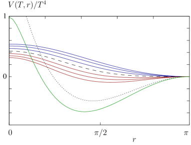
Figure 5: Rescaled two-loop background field potential $V(T,r)/T^{4}$ for various temperatures, below (blue) and above (red) the critical temperature (dashed black). The green curve corresponds to a higher temperature and shows the approach to the asymptotic high temperature limit $v_{\infty}(r)$ (dotted line); see Eq. (67). All curves have been shifted by their respective values at $r=\pi$ for clarity.

As already mentioned, we shall use the values of $m$ and $g$ inferred from lattice calculations of ghost and gluon propagators in the Landau gauge at vanishing temperature. For the present order of approximation, we fit these data to the one-loop expressions obtained in the massive Landau gauge. The best fitting values are $m\simeq 680$ MeV and $g\simeq 7.5$ with $\mu=1$ GeV. This sets the scale of the present calculation. We shall compare our findings to our earlier leading-order results Reinosa:2014ooa where the mass parameter was obtained by fitting the data to the tree-level propagators with the best fitting value $m\simeq 710$ MeV. There is of course some error related to the determination of the parameters. We have checked that the results to be presented below do not change qualitatively as we change the parameters within the error bars. Let us finally mention that we shall not consider the possible temperature dependence of the parameters. This and the implementation of renormalization-group improvement are deferred to a future work.

VI.1 Background field potential

In Fig. 5, we show the rescaled two-loop background field potential $V(T,r)/T^{4}$ in the range $[0,\pi]$ for various values of the temperature. As the temperature is increased, there is clearly a transition from a confining phase, where the minimum of the potential lies at its confining value $r=\pi$, to a deconfined phase where the location of the minimum departs from $r=\pi$. The transition is second order and the corresponding critical temperature is obtained by requiring the vanishing of the curvature of the potential at the confining point. The rescaled curvature $\partial_{r}^{2}V(T,r)/T^{4}$ at $r=\pi$ is plotted as a function of $T$ in the left panel of Fig. 6 at one- and two-loop orders. The two-loop correction leads to a larger critical temperature, $T_{\rm c}^{\rm 2loop}\simeq 284\,{\rm MeV}$, as compared to our previous one-loop result Reinosa:2014ooa , $T_{\rm c}^{\rm 1loop}\simeq 237\,{\rm MeV}$. A typical lattice result is Lucini:2012gg $T_{c}^{\rm latt}=295$ MeV. Although such comparison must be taken with care due to the issue of properly setting the scale, this shows that the two-loop corrections indeed improve the one-loop result.

It is also interesting to compare with other continuum approaches. The FRG and DSE/2PI calculations of Ref. Fister:2013bh give $T_{c}^{\rm FRG}=230\,{\rm MeV}$ and $T_{c}^{\rm DSE/2PI}=235\,{\rm MeV}$, respectively, which lie in the same ballpark as our one-loop result. The improved value of the critical temperature obtained above suggests that the present two-loop calculation efficiently captures some of the effects which have been discarded in those calculations. For instance, although the fully resummed propagators are included, some explicit two-loop contributions to the DSE for the background field potential have been neglected. As for the FRG calculation, the authors of Ref. Fister:2013bh mention that their result is modified to $T_{c}^{\rm FRG}=300\,{\rm MeV}$ when some backreaction effects—neglected in their main study—are included.

For completeness, we compare in Fig. 7 the one- and two-loop potentials at their respective critical temperatures. It is also instructive to plot the (rescaled) curvature of the potential at the origin as a function of $T$; see the right panel of Fig. 6. For the values of parameters studied here, we observe that, at one-loop order, there exists a temperature $T_{\star}\simeq 1.5T^{\rm 1loop}_{\rm c}$ above which the minimum of the potential is exactly located at $r=0$. This does not seem to be the case at two-loop order where the curvature of the potential at the origin remains negative.

To have a better analytical control on our results, we have considered the formal limit $T\to\infty$. We show in Appendix D.3 that the rescaled potential $v_{\infty}(r)=\lim_{T\to\infty}V(T,r)/T^{4}$ is a polynomial in the range $[0,\pi]$:

$$v_{\infty}(r) = \frac{\pi^{2}}{60}\left[5\left(\frac{r}{\pi}-1\right)^{4}-10\left(\frac{r}{\pi}-1\right)^{2}+1\right]$$ (67)

$$+ \frac{g^{2}}{96}\left[7\left(\frac{r}{\pi}-1\right)^{4}-2\left(\frac{r}{\pi}-1\right)^{2}-1\right],$$

which minimum is located at

$$r_{\infty}=\pi\left(1-\sqrt{\frac{8\pi^{2}+g^{2}}{8\pi^{2}+7g^{2}}}\right).$$ (68)

We discuss the consequences of the different behavior between the one- and two-loop results below.

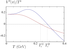
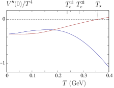
Figure 6: Rescaled curvature of the one-loop (red) and two-loop (blue) background potentials at $r=\pi$ (left) and $r=0$ (right) as functions of the temperature. The curvatures at $r=\pi$ vanish at the corresponding critical temperatures, denoted here by $T_{c}^{1l}$ and $T_{c}^{2l}$, respectively. The one-loop curvature at $r=0$ vanishes at a temperature $T_{\star}$, above which the minimum of the one-loop potential is at $r=0$. This does not happen at two loops.

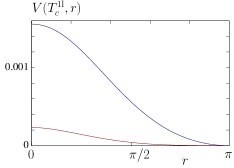
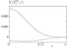
Figure 7: One-loop (red) and two-loop (blue) background field potentials as functions of $r$ at $T=T_{\rm c}^{\rm 1loop}$ (left) and $T=T_{\rm c}^{\rm 2loop}$ (right). The curves have been shifted by their respective values at $r=\pi$ for clarity.

VI.2 Polyakov loop

In Fig. 8, we compare the temperature dependence of the Polyakov loop at leading and next-to-leading order. At leading order, it saturates to its upper bound $\ell^{(0)}_{\infty}=1$ at the temperature $T_{\star}$ discussed previously, above which $r=0$ remains the absolute minimum of the potential; see Fig. 6. The Polyakov loop is singular at $T=T_{\star}$ because its second derivative is discontinuous. This has to do with the particular form of the Weiss potential, Eq. (IV.1). For small positive values of $r$, the latter behaves as

$${\cal F}_{0}(T,r)=T^{4}\left[-\frac{\pi^{2}}{15}+\frac{r^{2}}{3}-\frac{r^{3}}{3\pi}\dots\right]$$ (69)

and is thus nonanalytic in $r^{2}$. This is to be contrasted with the massive version ${\cal F}_{m}(T,r)$ of the same function which shows a regular expansion in powers of $r^{2}$ when $m\neq 0$. In the vicinity of $r=0$ and for $T$ close to $T_{\star}$, the rescaled potential is of the form $a(T)+b(T)r^{2}+cr^{3}$, where $b(T)=b_{-}(T_{\star}-T)$ with $b_{-}<0$ and $c>0$. It follows, that for $T$ approaching $T_{\star}$ from below, $r(T)\propto T_{\star}-T$ and $r(T)=0$ for $T>T_{\star}$. Thus, the first derivative of the background with respect to the temperature is discontinuous at $T=T_{\star}$. This singularity propagates to thermodynamic observables. For instance the third derivative of the free energy density with respect to the temperature is discontinuous. This is, however, a spurious discontinuity.

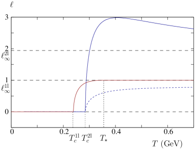
Figure 8: Temperature dependence of the Polyakov loop at leading (red) and next-to-leading (blue) orders. The horizontal dashed lines denote the corresponding asymptotic values at high temperature, denoted here by $\ell_{\infty}^{1l}$ and $\ell_{\infty}^{2l}$, respectively. The dashed blue curve shows the mean-field Polyakov loop (63) evaluated at $r=r_{\rm min}^{\rm 2loop}$.The respective one- and two-loop critical temperatures are indicated by vertical dashed lines, as well as the temperature $T_{\star}$ at which the leading-order Polyakov loop reaches its asymptotic value.

As already discussed above, at two-loop order the curvature of the potential at the origin remains negative. In this range, the Polyakov loop does not show any additional singularity, other than the one at $T^{\rm 2loop}_{\rm c}$. We also observe that, as compared to the one-loop result, the Polyakov loop at two-loop order overshoots its asymptotic ($T\to\infty$) value

$$\ell^{\rm 1loop}_{\infty}=\cos\left(\frac{r_{\infty}}{2}\right)+\frac{3g^{2}}{16\pi^{2}}(\pi-r_{\infty})\sin\left(\frac{r_{\infty}}{2}\right),$$ (70)

with $r_{\infty}$ given in (68), as computed in Appendix E.

VI.3 Pressure and entropy

The thermodynamic pressure (14) is shown in Fig. 9 as a function of the temperature in the one- and two-loop approximations. In both cases, we observe that the pressure is increasing at small temperatures, indicating a positive entropy ($s=dp/dT$). This is a welcome result although it may be surprising at first sight because the ghosts dominate in this regime and one would naively think that they contribute negatively to the entropy.

The positivity of the entropy at low temperatures is ensured by the fact that, in the confining phase with $r=\pi$, those ghosts which feel the background effectively behave as physical fermions, giving a positive contribution to the entropy. To illustrate this point more precisely, we note that the low temperature behavior of the background field potential is dominated by the one-loop contribution, as discussed in Appendix D. This is directly visible in Fig. 10. At one-loop order, in the confined phase, the entropy contribution $\Delta_{\kappa}s$ of a ghost with charge $\kappa$ is

$$\frac{\Delta_{\kappa}s}{2T^{3}}=\int_{\bf q}\ln\Big{(}1+e^{-2q}-2e^{-q}\cos(\kappa\pi)\Big{)}.$$ (71)

So we have either a bosoniclike contribution ($d=4$)

$$\frac{\Delta_{0}s}{4T^{3}}=\int_{\bf q}\ln\Big{(}1-e^{-q}\Big{)}=-\frac{\pi^{2}}{90}\,,\\$$ (72)

with a standard negative (ghostlike) sign from the neutral modes, or fermioniclike contributions

$$\frac{\Delta_{\pm}s}{4T^{3}}=\int_{\bf q}\ln\Big{(}1+e^{-q}\Big{)}=\frac{7\pi^{2}}{720}$$ (73)

with a positive sign for charged modes due to their coupling to the background. The total ghost contribution,

$$\frac{\Delta_{0}s+2\Delta_{+}s}{4T^{3}}=\frac{\pi^{2}}{120},$$ (74)

is then positive, as announced.

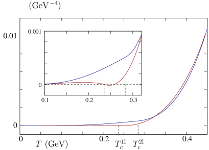
Figure 9: Thermodynamic pressure at one- (red) and two-loop (blue) orders, obtained from the minimum of the background field potential as a function of the temperature. The plot in the inset is a zoom on the low temperature region. The respective one- and two-loop critical temperatures are indicated by vertical dashed lines.

As one increases the temperature, the one-loop result violates the positivity of the entropy, slightly before reaching $T_{\rm c}^{\rm 1loop}$, as can be clearly seen in the inset plot of Fig. 9, where the thermal pressure changes its monotony and even becomes slightly negative before $T_{\rm c}^{\rm 1loop}$. The reason for this behavior is again the change of effective statistics of the relevant degrees of freedom in the presence of the background. As the temperature is increased, the massive gluons start contributing to the pressure. However, in the confined phase, the charged gluons, which feel the presence of the background, behave like “wrong” fermions, contributing negatively to the entropy Sasaki:2012bi . Remarkably this behavior is completely washed out by the two-loop correction and at two-loop order the entropy is positive (the pressure is monotonically increasing with the temperature) in the whole range of temperatures studied here; see Fig. 9.

Finally, let us comment on the $T^{4}$ behavior of the pressure at low temperature—see Fig. 10—which is at odds with the exponential suppression seen in lattice results Engels:1981qx . As discussed above, this originates from the fact that massless (ghost) modes directly contribute to the pressure, already at leading order. We mention that this is likely to be a general problem for continuum approaches, which are essentially based on using (resummed) propagators. For instance, in the Landau gauge, lattice results for the propagators Boucaud:2011ug ; Maas:2011se show that, if the gluon becomes effectively massive for infrared momenta, the ghost remains massless. This generically produces $T^{4}$ contributions in a leading-order-like—i.e., trace-log—expression for the thermodynamic pressure. The correct treatment of such unphysical massless degrees of freedom is a serious issue that needs to be further investigated.

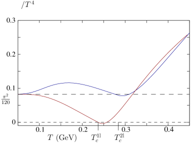
Figure 10: Thermodynamic pressure rescaled by $T^{4}$, at one-loop (red) and two-loop (blue) orders, as a function of temperature.

VI.4 Comparison with the massive Landau gauge

It is interesting to compare our results for the pressure to those obtained in the massive Landau gauge (which corresponds to a vanishing background). The corresponding one- and two-loop pressure curves are shown in Fig. 11 and compared to those discussed in the previous subsection. We observe again that the one-loop pressure contains $T^{4}$ contributions at low temperatures but this time those come with a negative prefactor which yields a negative entropy at low temperatures. The reason for this is simple: in the absence of background all ghosts contribute negatively to the entropy. In this case the two-loop correction is of no help because it does not contain any $T^{4}$ contribution at small temperature. In fact it seems that the two-loop term makes the problem even worse since the entropy remains negative in the range of temperature shown here. Furthermore, we observe in Fig. 11 that the two-loop correction is smaller in the Landau-DeWitt case than in the Landau case, indicating a better convergence.

The above remarks illustrate the importance of taking into account the order parameter of the $Z_{N}$ transition in the description. Our two-loop results show that the value $r=0$—which would correspond to the Landau gauge—is never a physical point, i.e., an absolute minimum of the background field potential. In a sense, the perturbative expansion in the (massive) Landau gauge appears as an expansion around an unstable situation. It would take infinite resummations to correctly describe the physics near the stable physical point.We believe that this remark outranges the present framework and holds for other continuum approaches as well.

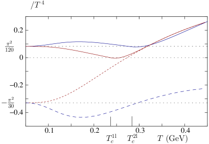
Figure 11: Comparison between one-loop (red) and two-loop (blue) results in the massive Landau-DeWitt gauge (plain) and in the massive Landau gauge (dashed). Both one-loop results coincide for $T>T_{\star}$ (see text) because in that case $r=0$. The critical temperatures indicated on the horizontal axis are those obtained from the Landau-DeWitt calculation.

VII Conclusions

To summarize, we have proposed in Reinosa:2014ooa a perturbative approach to describe the static quark confinement-deconfinement transition in Yang-Mills theories, based on a modified (massive) gauge-fixed action in the Landau-DeWitt gauge. This describes well the phase structure of SU($N$) theories at leading order and gives qualitatively good results for the transition temperatures of the $N=2$ and $N=3$ cases in $d=4$. However, this leads to a $T^{4}$ behavior of the thermodynamic pressure at low temperatures and to negative entropy and negative pressure near the transition temperature. Also the leading-order calculation leads to a spurious singularity at a temperature $T_{\star}$ above which the physical background field vanishes.

With the present work, we wish to demonstrate the interest and feasibility of a next-to-leading-order calculation in this modified perturbative scheme. We investigate the SU($2$) theory at next-to-leading order, which shows that the correction to the critical temperature goes in the right direction and actually brings the estimated value close to the lattice result—although we stress again that such a comparison must be taken with care due to the issue of scale setting. The next-to-leading-order corrections also cure the negative entropy issue and remove the spurious singularity at $T=T_{\star}$. In fact, we find that the physical point always corresponds to a nonvanishing background field. There remains the issue of unphysical $T^{4}$ contributions to the pressure from the massless (ghost) degrees of freedom, which needs to be investigated.

In a future work, we shall extend the present two-loop study to the SU($3$) theory and investigate the effect of renormalization-group improvement. Another interesting extension would be to include quark degrees of freedom at nonzero chemical potential. Finally, the present work points out the importance of taking into account a nonvanishing background field near the phase transition. We plan to extend our previous study Reinosa:2013twa of the Landau gauge ghost and gluon correlators at finite temperature to the Landau-DeWitt gauge.

Appendix A Gluon loops

Here, we detail the derivation of Eqs. (50) and (IV.2) for the purely gluonic two-loop diagrams. A straightforward application of the Feynman rules of Sec. III.3 yields, for the double gluon tadpole diagram (first diagram of Fig. 4),

$$V^{(2)}_{\rm 2g}=-\frac{g^{2}}{8} \sum_{\kappa,\lambda,\omega}\int_{Q,K}G_{\mu\nu}(Q_{\kappa})G_{\rho\sigma}(K_{\lambda})$$

$$\times\Big{[}\,\, \varepsilon^{\kappa(-\kappa)\omega}\varepsilon^{(-\omega)\lambda(-\lambda)}(\delta_{\mu\rho}\delta_{\nu\sigma}-\delta_{\mu\sigma}\delta_{\nu\rho})$$

$$+\, \varepsilon^{\kappa\lambda\omega}\varepsilon^{(-\omega)(-\kappa)(-\lambda)}(\delta_{\mu\nu}\delta_{\rho\sigma}-\delta_{\mu\sigma}\delta_{\nu\rho})$$

$$+\, \varepsilon^{\kappa(-\lambda)\omega}\varepsilon^{(-\omega)\lambda(-\kappa)}(\delta_{\mu\rho}\delta_{\nu\sigma}-\delta_{\mu\nu}\delta_{\rho\sigma})\Big{]}.$$ (75)

The contribution from the first line in the brackets vanishes and the two other lines contribute the same. Setting $\lambda\to-\lambda$ and $K\to-K$ in the third line and using (25) and $G_{\rho\sigma}(-K_{\lambda})=G_{\rho\sigma}(K_{\lambda})$, we obtain

$$V^{(2)}_{\rm 2g} =\frac{g^{2}}{4}\sum_{\kappa,\lambda,\tau}{\cal C}_{\kappa\lambda\tau}\int_{Q,K}G_{m}(Q_{\kappa})G_{m}(K_{\lambda})$$

$$\times\Big{[}{\cal P}^{\perp}_{\mu\mu}(Q_{\kappa}){\cal P}^{\perp}_{\nu\nu}(K_{\lambda})-{\cal P}^{\perp}_{\mu\nu}(Q_{\kappa}){\cal P}^{\perp}_{\mu\nu}(K_{\lambda})\Big{]},$$ (76)

where we renamed $\omega\to\tau$ and we used the definition (42). This rewrites as Eq. (50) using the integrals (51) and (52). As mentioned in Sec. IV.2 for the ghost-gluon sunset diagram, we observe that the expression (A) can be obtained from the corresponding diagram at vanishing background field by replacing the loop momenta by shifted ones and by averaging with the weight ${\cal C}_{\kappa\lambda\tau}$, where, here, the index $\tau$ is redundant since it is not associated to any internal momentum.

A similar writing applies to the gluon sunset diagram (third diagram of Fig. 4). Applying the Feynman rules of Sec. III.3, we obtain, after simple manipulations,

$$V^{(2)}_{\rm 3g}=-g^{2}\sum_{\kappa,\lambda,\tau}{\cal C}_{\kappa\lambda\tau}\int_{Q,K}{\cal B}(Q_{\kappa},K_{\lambda},L_{\tau})G_{m}(Q_{\kappa})G_{m}(K_{\lambda})G_{m}(L_{\tau}),$$ (77)

where $Q+K+L=0$ and

$${\cal B}(Q,K,L)=\left[Q\cdot{\cal P}^{\perp}(L)\cdot Q\right]\hbox{tr}\left[{\cal P}^{\perp}(K){\cal P}^{\perp}(Q)\right]-2L\cdot{\cal P}^{\perp}(Q)\cdot{\cal P}^{\perp}(L)\cdot{\cal P}^{\perp}(K)\cdot L\,.$$ (78)

As emphasized previously, because ${\cal C}_{\kappa\lambda\tau}=0$ for $\kappa+\lambda+\tau\neq 0$, the sum of shifted momenta in (77) vanishes: $Q_{\kappa}+K_{\lambda}+L_{\tau}=0$. This allows us to use a number of manipulations similar to those used in the case of a vanishing background field. First, we symmetrize the function ${\cal B}$ under the momentum integral in (77) and use the identity

$$\frac{1}{6}\left\{{\cal B}(Q,K,L)+{\rm perm.}\right\}=\frac{1}{3}\left\{\left(d-\frac{3}{2}\right)\left(\frac{1}{K^{2}}+\frac{1}{Q^{2}}+\frac{1}{L^{2}}\right)+\frac{K^{4}+L^{4}+Q^{4}}{4Q^{2}L^{2}K^{2}}\right\}\left[L^{2}K^{2}-\left(L\cdot K\right)^{2}\right],$$ (79)

where “perm.” denotes all possible permutations of the momenta $Q$, $K$, and $L$. Note that, for $Q+K+L=0$, the last factor on the right-hand side is symmetric in $Q,K,L$; that is,

$$L^{2}K^{2}-\left(L\cdot K\right)^{2}=Q^{2}K^{2}-\left(Q\cdot K\right)^{2}=L^{2}Q^{2}-\left(L\cdot Q\right)^{2}.$$ (80)

Next, we “desymmetrize” the right-hand side of Eq. (79) under the integral in (77), which amounts to replacing

$${\cal B}(Q_{\kappa},K_{\lambda},L_{\tau})\to\left\{\left(d-\frac{3}{2}\right)\frac{1}{Q_{\kappa}^{2}}+\frac{Q_{\kappa}^{2}}{4L_{\tau}^{2}K_{\lambda}^{2}}\right\}\left[L_{\tau}^{2}K_{\lambda}^{2}-\left(L_{\tau}\cdot K_{\lambda}\right)^{2}\right]$$ (81)

in (77). The momentum integral in Eq. (77) can thus be written

$$\int_{Q,K}\left[L_{\tau}^{2}K_{\lambda}^{2}-(L_{\tau}\cdot K_{\lambda})^{2}\right]\left\{\left(d-\frac{3}{2}\right)\frac{G_{m}(Q_{\kappa})}{Q_{\kappa}^{2}}G_{m}(K_{\lambda})G_{m}(L_{\tau})+\frac{1}{4}\left[1-m^{2}G_{m}(Q_{\kappa})\right]\frac{G_{m}(K_{\lambda})}{K_{\lambda}^{2}}\frac{G_{m}(L_{\tau})}{L_{\tau}^{2}}\right\},$$ (82)

where we used $Q^{2}G_{m}(Q)=1-m^{2}G_{m}(Q)$. Using the trick (46) as well as the symmetry properties of the tensor (42) and of the integral (48), we obtain Eq. (IV.2), after some simple manipulations.

Appendix B Reduction of the integral $I^{\kappa\lambda\tau}_{\alpha\beta\gamma}$ to the integrals $J^{\kappa}_{\alpha}$, $\tilde{J}^{\kappa}_{\alpha}$, and $S^{\kappa\lambda\tau}_{\alpha\beta\gamma}$

Here, we show how the integral $I^{\kappa\lambda\tau}_{\alpha\beta\gamma}$, Eq. (48), can be expressed in terms of the scalar tadpole and sunset loop integrals $J_{\alpha}^{\kappa}$, $\tilde{J}_{\alpha}^{\kappa}$ and $S^{\kappa\lambda\tau}_{\alpha\beta\gamma}$ given in Eqs. (51), (59), and (60), respectively. To do so, we work out the various pieces of the integrand in Eq. (48). We first write

$$Q^{2}K^{2}G_{\alpha}(Q)G_{\beta}(K) =(Q^{2}+\alpha^{2}-\alpha^{2})(K^{2}+\beta^{2}-\beta^{2})G_{\alpha}(Q)G_{\beta}(K)$$

$$=1-\left[\alpha^{2}G_{\alpha}(Q)+\beta^{2}G_{\beta}(K)\right]+\alpha^{2}\beta^{2}G_{\alpha}(Q)G_{\beta}(K)\,,$$ (83)

and, using the identity

$$Q\cdot K=\frac{1}{2}\Big{[}\alpha^{2}+\beta^{2}-\gamma^{2}+L^{2}+\gamma^{2}-(Q^{2}+\alpha^{2})-(K^{2}+\beta^{2})\Big{]},$$ (84)

we also have

$$(Q\cdot K)^{2}G_{\alpha}(Q)G_{\beta}(K)G_{\gamma}(L) =\left(\frac{\alpha^{2}+\beta^{2}-\gamma^{2}}{2}\right)^{2}G_{\alpha}(Q)G_{\beta}(K)G_{\gamma}(L)$$

$$+\frac{1}{2}\left(\frac{\alpha^{2}+\beta^{2}-\gamma^{2}}{2}+Q\cdot K\right)\Big{\{}G_{\alpha}(Q)G_{\beta}(K)-\left[G_{\alpha}(Q)+G_{\beta}(K)\right]G_{\gamma}(L)\Big{\}}\,.$$ (85)

Combining the above identities, we obtain

$$\left[Q^{2}K^{2}-\left(Q\cdot K\right)^{2}\right] G_{\alpha}(Q)G_{\beta}(K)G_{\gamma}(L)$$

$$=\frac{1}{2}\Big{\{}2+Q\cdot K\left[G_{\alpha}(Q)+G_{\beta}(K)\right]\Big{\}}G_{\gamma}(L)-\frac{Q\cdot K}{2}G_{\alpha}(Q)G_{\beta}(K)$$

$$-\frac{1}{4}(\alpha^{4}+\beta^{4}+\gamma^{4}-2\alpha^{2}\beta^{2}-2\alpha^{2}\gamma^{2}-2\beta^{2}\gamma^{2})G_{\alpha}(Q)G_{\beta}(K)G_{\gamma}(L)$$

$$+\frac{\gamma^{2}-\alpha^{2}-\beta^{2}}{4}G_{\alpha}(Q)G_{\beta}(K)+\frac{\beta^{2}-3\alpha^{2}-\gamma^{2}}{4}G_{\alpha}(Q)G_{\gamma}(L)+\frac{\alpha^{2}-3\beta^{2}-\gamma^{2}}{4}G_{\beta}(K)G_{\gamma}(L)\,.$$

The term in curly brackets on the right-hand side can be rewritten as

$$\Big{[}1+Q\cdot KG_{\alpha}(Q)\Big{]}+\Big{[}1+Q\cdot KG_{\beta}(K)\Big{]}=\left(\alpha^{2}-Q\cdot L\right)G_{\alpha}(Q)+\left(\beta^{2}-K\cdot L\right)G_{\beta}(K),$$ (87)

where we used the fact that $Q+K+L=0$, which, as already emphasized, holds as well for the shifted momenta in Eq. (48) under the average with weight ${\cal C}_{\kappa\lambda\tau}$. Inserting (87) in (B), we obtain the following, manifestly symmetric expression for the integrand in (48):

$$4\left[Q^{2}K^{2}-\left(Q\cdot K\right)^{2}\right]G_{\alpha}(Q)G_{\beta}(K)G_{\gamma}(L) =\left(2\alpha^{2}\beta^{2}+2\alpha^{2}\gamma^{2}+2\beta^{2}\gamma^{2}-\alpha^{4}-\beta^{4}-\gamma^{4}\right)G_{\alpha}(Q)G_{\beta}(K)G_{\gamma}(L)$$

$$+\left(\gamma^{2}-\alpha^{2}-\beta^{2}-2Q\cdot K\right)G_{\alpha}(Q)G_{\beta}(K)$$

$$+\left(\alpha^{2}-\beta^{2}-\gamma^{2}-2K\cdot L\right)G_{\beta}(K)G_{\gamma}(L)$$

$$+\left(\beta^{2}-\gamma^{2}-\alpha^{2}-2L\cdot Q\,\right)G_{\gamma}(L)G_{\alpha}(Q).$$ (88)

It is then immediate to obtain the desired relation:

$$I^{\kappa\lambda\tau}_{\alpha\beta\gamma} =\frac{1}{4}\left[\left(\gamma^{2}-\alpha^{2}-\beta^{2}\right)J_{\alpha}^{\kappa}J_{\beta}^{\lambda}+\left(\beta^{2}-\alpha^{2}-\gamma^{2}\right)J_{\alpha}^{\kappa}J_{\gamma}^{\tau}+\left(\alpha^{2}-\beta^{2}-\gamma^{2}\right)J_{\beta}^{\lambda}J_{\gamma}^{\tau}\right]$$

$$-\frac{1}{2}\Big{[}\tilde{J}_{\alpha}^{\kappa}\tilde{J}_{\beta}^{\lambda}+\tilde{J}_{\alpha}^{\kappa}\tilde{J}_{\gamma}^{\tau}+\tilde{J}_{\beta}^{\lambda}\tilde{J}_{\gamma}^{\tau}\Big{]}-\frac{1}{4}\left(\alpha^{4}+\beta^{4}+\gamma^{4}-2\alpha^{2}\beta^{2}-2\alpha^{2}\gamma^{2}-2\beta^{2}\gamma^{2}\right)S^{\kappa\lambda\tau}_{\alpha\beta\gamma}\,,$$ (89)

where we used

$$\int_{Q,K}\left(Q_{\kappa}\cdot K_{\lambda}\right)G_{\alpha}(Q_{\kappa})G_{\beta}(K_{\lambda})=\int_{Q}Q_{\kappa}^{0}G_{\alpha}(Q_{\kappa})\int_{K}K_{\lambda}^{0}G_{\beta}(K_{\lambda})=\tilde{J}_{\alpha}^{\kappa}\tilde{J}_{\beta}^{\lambda}.$$ (90)

The relation (89) reads, explicitly, for the various cases of interest,

$$I^{\kappa\lambda\tau}_{mmm} = -\frac{1}{2}\big{[}\tilde{J}_{m}^{\kappa}\tilde{J}_{m}^{\lambda}+\tilde{J}_{m}^{\kappa}\tilde{J}_{m}^{\tau}+\tilde{J}_{m}^{\lambda}\tilde{J}_{m}^{\tau}\big{]}-\frac{m^{2}}{4}\big{[}J_{m}^{\kappa}J_{m}^{\lambda}+J_{m}^{\kappa}J_{m}^{\tau}+J_{m}^{\lambda}J_{m}^{\tau}\big{]}+\frac{3m^{4}}{4}S_{mmm}^{\kappa\lambda\tau}$$ (91)

$$I^{\kappa\lambda\tau}_{m00} = -\frac{1}{2}\big{[}\tilde{J}_{m}^{\kappa}\tilde{J}_{0}^{\lambda}+\tilde{J}_{m}^{\kappa}\tilde{J}_{0}^{\tau}+\tilde{J}_{0}^{\lambda}\tilde{J}_{0}^{\tau}\big{]}-\frac{m^{2}}{4}\left[J_{m}^{\kappa}J_{0}^{\lambda}+J_{m}^{\kappa}J_{0}^{\tau}-J_{0}^{\lambda}J_{0}^{\tau}\right]-\frac{m^{4}}{4}S^{\kappa\lambda\tau}_{m00}$$ (92)

$$I^{\kappa\lambda\tau}_{mm0} = -\frac{1}{2}\big{[}\tilde{J}_{m}^{\kappa}\tilde{J}_{m}^{\lambda}+\tilde{J}_{m}^{\kappa}\tilde{J}_{0}^{\tau}+\tilde{J}_{m}^{\lambda}\tilde{J}_{0}^{\tau}\big{]}-\frac{m^{2}}{2}J_{m}^{\kappa}J_{m}^{\lambda}$$ (93)

$$I^{\kappa\lambda\tau}_{000} = -\frac{1}{2}\big{[}\tilde{J}_{0}^{\kappa}\tilde{J}_{0}^{\lambda}+\tilde{J}_{0}^{\kappa}\tilde{J}_{0}^{\tau}+\tilde{J}_{0}^{\lambda}\tilde{J}_{0}^{\tau}\big{]}.$$ (94)

Using these relations in Eq. (58), we obtain Eq. (61).

Appendix C Matsubara sums

In this section, we perform explicitly the various sums over Matsubara frequencies and angular momentum integrations involved in the one- and two-loop scalar integrals derived in the previous section and we extract the UV divergent parts using dimensional regularization. In what follows, we note $\hat{r}=rT$, such that shifted momenta read $Q_{\kappa}=(\omega_{n}+\kappa\hat{r},\bf q\,)$.

C.1 Tadpoles

We begin with the tadpole integral

$$J^{\kappa}_{\alpha}=\int_{Q}G_{\alpha}(Q_{\kappa})\,.$$ (95)

Note that $J_{\alpha}^{\kappa}=J_{\alpha}^{-\kappa}$. Standard contour integration techniques yield

$$J^{\kappa}_{\alpha} =\mu^{2\epsilon}\int_{\bf q}\frac{1}{2\varepsilon_{\alpha,q}}[n_{\varepsilon_{\alpha,q}-i\kappa\hat{r}}-n_{-\varepsilon_{\alpha,q}-i\kappa\hat{r}}]$$

$$=J^{\rm vac}_{\alpha}+\int_{\bf q}\,{\rm Re}\,\frac{n_{\varepsilon_{\alpha,q}-i\kappa\hat{r}}}{\varepsilon_{\alpha,q}}\,,$$ (96)

where $\int_{\bf q}=\int\frac{d^{d-1}q}{(2\pi)^{d-1}}$, $\varepsilon_{\alpha,q}=\sqrt{q^{2}+\alpha^{2}}$, and $n_{z}=(\exp\beta z-1)^{-1}$ is the Bose-Einstein distribution function, which satisfies $n_{-x}=-1-n_{x}$. Here, we extracted explicitly a zero temperature, background-field-independent contribution $J^{\rm vac}_{\alpha}$. For later use, we introduce the following notation

$$J^{\kappa}_{\alpha}=J_{\alpha}(0n)+J^{\kappa}_{\alpha}(1n),$$ (97)

which emphasizes the number of thermal factors (i.e., Bose-Einstein distribution functions) appearing in each term on the right-hand side of (96). In particular, $J_{\alpha}(0n)=J^{\rm vac}_{\alpha}$. In dimensional regularization $J_{0}(0n)=0$ and

$$J_{m}(0n) =\mu^{2\epsilon}\int_{\bf q}\frac{1}{2\varepsilon_{q}}=\mu^{2\epsilon}\int\frac{d^{d}Q}{(2\pi)^{d}}\frac{1}{Q^{2}+m^{2}}$$

$$=-\frac{m^{2}}{16\pi^{2}}\left[\frac{1}{\epsilon}+\ln\frac{\bar{\mu}^{2}}{m^{2}}+1+{\cal O}(\epsilon)\right],$$ (98)

where $\bar{\mu}^{2}=4\pi e^{-\gamma}\mu^{2}$, with $\gamma$ the Euler constant.

The other tadpole integral which appears in Eq. (61) is

$$\tilde{J}^{\kappa}_{\alpha}=\int_{Q}Q^{0}_{\kappa}G_{\alpha}(Q_{\kappa}).$$ (99)

The Matsubara sum in this expression is not absolutely convergent but it can be defined as the limit of the symmetric summation $\sum_{n=-N}^{N}$ for $N\to\infty$. Alternatively, we can make it an absolutely convergent sum by writing

$$\sum_{n=-N}^{N}Q_{\kappa}^{0}G_{\alpha}(Q_{\kappa})=\sum_{n=-N}^{N}\Big{[}Q_{\kappa}^{0}G_{\alpha}(Q_{\kappa})-Q^{0}G_{\alpha}(Q)\Big{]},$$ (100)

where the added term vanishes by symmetry. We can then use standard contour techniques to obtain

$$\tilde{J}^{\kappa}_{\alpha} =\int_{\bf q}\frac{1}{2i}\Big{[}n_{\varepsilon_{\alpha,q}-i\kappa\hat{r}}+n_{-\varepsilon_{\alpha,q}-i\kappa\hat{r}}-n_{\varepsilon_{\alpha,q}}-n_{-\varepsilon_{\alpha,q}}\Big{]}$$

$$=\int_{\bf q}\,{\rm Im}\,n_{\varepsilon_{\alpha,q}-i\kappa\hat{r}}\,,$$ (101)

which satisfies $\tilde{J}^{-\kappa}_{\alpha}=-\tilde{J}^{\kappa}_{\alpha}$ and, in particular, $\tilde{J}_{\alpha}^{0}=0$. The zero temperature contribution vanishes identically, $\tilde{J}^{\kappa}_{\alpha}(0n)=0$, and we also note that $\tilde{J}^{\kappa}_{\alpha}=0$ when $r$ is a multiple of $\pi$. The integral (101) is finite and never multiplies a divergent contribution, so we can safely set $d\to 4$ there.

C.2 The scalar sunset

We now treat the scalar two-loop integral

$$S^{\kappa\lambda\tau}_{\alpha\beta\gamma}\equiv\int_{Q,K}G_{\alpha}(Q_{\kappa})G_{\beta}(K_{\lambda})G_{\gamma}(L_{\tau})\,,$$ (102)

where $Q+K+L=0$, for the relevant case of conserved shifts, $\kappa+\lambda+\tau=0$, which implies $Q_{\kappa}+K_{\lambda}+L_{\tau}=0$. We extend the approach of Blaizot:2004bg . It proves useful to introduce the spectral representation of the (free) propagators

$$G_{\alpha}(Q_{\kappa})=\tilde{G}_{\alpha}(i\omega_{n}^{\kappa};q)\equiv\int_{q_{0}}\frac{\rho_{\alpha}(q_{0},q)}{q_{0}-i\omega_{n}^{\kappa}},$$ (103)

where $\int_{q_{0}}=\int dq_{0}/(2\pi)$, $\omega_{n}^{\kappa}=\omega_{n}+\kappa\hat{r}$ is the shifted Matsubara frequency, and

$$\rho_{\alpha}(q_{0},q)=2\pi\,{\rm sign}(q_{0})\delta\!\left(q^{2}_{0}-\varepsilon_{\alpha,q}^{2}\right),$$ (104)

with $\varepsilon_{\alpha,q}=\sqrt{q^{2}+\alpha^{2}}$. The double Matsubara sum in (102) yields

$$T^{2}\sum_{n,m}\frac{1}{(q_{0}-i\omega_{n}^{\kappa})(k_{0}-i\omega_{m}^{\lambda})(l_{0}+i\omega_{n}^{\kappa}+i\omega_{m}^{\lambda})}\,.$$

$$\hskip 14.22636pt=\,\frac{(n_{k_{0}-i\lambda\hat{r}}-n_{-l_{0}+i\tau\hat{r}})(n_{q_{0}-i\kappa\hat{r}}-n_{-l_{0}-k_{0}-i\kappa\hat{r}})}{l_{0}+k_{0}+q_{0}}$$

$$\hskip 14.22636pt=\,\frac{n_{k_{0}-i\lambda\hat{r}}n_{l_{0}-i\tau\hat{r}}-n_{-q_{0}+i\kappa\hat{r}}(n_{k_{0}-i\lambda\hat{r}}-n_{-l_{0}+i\tau\hat{r}})}{l_{0}+k_{0}+q_{0}},$$ (105)

where we have used the identity $(1+n_{x}+n_{y})n_{x+y}=n_{x}n_{y}$ and $\kappa+\lambda+\tau=0$. The second line of this equation makes it clear that (105) is well defined for all $k_{0}$, $q_{0}$, and $l_{0}$, including the limiting case $l_{0}+k_{0}+q_{0}\to 0$, for which both the numerator and the denominator vanish linearly. In the following, we shall decompose the fraction in the third line of (105) in different pieces whose numerators do not vanish at $l_{0}+k_{0}+q_{0}=0$, thus making the corresponding contribution to (105) formally divergent in this limit. To avoid this problem, we regulate the denominator in (105) as

$$\frac{1}{l_{0}+k_{0}+q_{0}}\to{\rm Re}\left(\frac{1}{l_{0}+k_{0}+q_{0}+i0^{+}}\right).$$ (106)

Now, we use the identities

$$n_{k_{0}-i\kappa\hat{r}} =-\theta(-k_{0})+{\rm sign}(k_{0})n_{|k_{0}|-i\,{\rm sign}(k_{0})\kappa\hat{r}}$$ (107)

$$n_{-k_{0}+i\kappa\hat{r}} =-\theta(k_{0})-{\rm sign}(k_{0})n_{|k_{0}|-i\,{\rm sign}(k_{0})\kappa\hat{r}}$$ (108)

in the third line of (105) to rewrite Eq. (102) as

$$S_{\alpha\beta\gamma}^{\kappa\lambda\tau} =S_{\alpha\beta\gamma}^{\rm vac}+\mu^{2\epsilon}\int_{q_{0},\bf q}\!\!\sigma_{\alpha}^{\kappa}(q_{0},q)\,{\rm Re}\,\tilde{I}_{\beta\gamma}(q_{0}+i0^{+};q)$$

$$+\int_{q_{0},k_{0},\bf q,\bf k}\sigma_{\alpha}^{\kappa}(q_{0},q)\sigma_{\beta}^{\lambda}(k_{0},k)\,{\rm Re}\,\tilde{G}_{\gamma}(\ell_{0}+i0^{+};\ell)$$

$$+{\rm perm.},$$ (109)

where $S_{\alpha\beta\gamma}^{\rm vac}$ is an unimportant vacuum contribution, independent of the temperature and of the background field, $\ell_{0}=q_{0}+k_{0}$, $\ell=|\bf{q}+\bf{k}|$,

$$\sigma_{\alpha}^{\kappa}(q_{0},q)=\rho_{\alpha}(q_{0},q)\,{\rm sign}(q_{0})\,n_{|q_{0}|-i\,{\rm sign}(q_{0})\kappa\hat{r}},$$ (110)

and “perm.” denotes the circular permutations of the pairs of indices $(\alpha,\kappa)$, $(\beta,\lambda)$, and $(\gamma,\tau)$ in the two integrals that appear explicitly in (109). The function $\tilde{G}_{\alpha}(z;q)$ has been defined in (103) and the function $\tilde{I}_{\alpha\beta}(z;q)$ is related to the vacuum one-loop integral [here $Q=(\omega,\bf q)$]

$$I^{\rm vac}_{\alpha\beta}(Q) =\tilde{I}_{\alpha\beta}(i\omega;q)\equiv\mu^{2\epsilon}\!\!\int\frac{d^{d}K}{(2\pi)^{d}}G_{\alpha}(K)G_{\beta}(Q+K)$$

$$=\mu^{2\epsilon}\!\!\int_{k_{0},l_{0},\bf k}\rho_{\alpha}(k_{0},k)\rho_{\beta}(l_{0},\ell)\,\frac{\theta(l_{0})-\theta(-k_{0})}{i\omega+l_{0}+k_{0}}.$$ (111)

In obtaining Eq. (109), we have used $\tilde{G}_{\alpha}(x;q)=\tilde{G}_{\alpha}(-x;q)$ and $\tilde{I}_{\alpha\beta}(x;q)=\tilde{I}_{\alpha\beta}(-x;q)$, and we have set $d\to 4$ in the second, UV finite line. In contrast, one has to keep $d$ arbitrary in the second term on the right-hand side of Eq. (109) since it contains UV divergent contributions, arising from the zero temperature loop (111).

It is now an easy matter to perform explicitly the frequency and, for the double integral on the second line, the angular integrations. As before, we decompose the result according to the number of thermal factors $n$ in each contribution as

$$S_{\alpha\beta\gamma}^{\kappa\lambda\tau}=S_{\alpha\beta\gamma}^{\kappa\lambda\tau}(0n)+S_{\alpha\beta\gamma}^{\kappa\lambda\tau}(1n)+S_{\alpha\beta\gamma}^{\kappa\lambda\tau}(2n).$$ (112)

We obtain

$$S_{\alpha\beta\gamma}^{\kappa\lambda\tau}(1n) =\mu^{2\epsilon}\int_{\bf q}\,{\rm Re}\,\frac{n_{\varepsilon_{\alpha,q}-i\kappa\hat{r}}}{\varepsilon_{\alpha,q}}\,{\rm Re}\,\tilde{I}_{\beta\gamma}(\varepsilon_{\alpha,q}+i0^{+};q)+{\rm perm.}$$ (113)

$$S_{\alpha\beta\gamma}^{\kappa\lambda\tau}(2n) =\frac{1}{32\pi^{4}}\int_{0}^{\infty}\!\!dq\,q\int_{0}^{\infty}\!\!dk\,k\,{\rm Re}\,\frac{n_{\varepsilon_{\alpha,q}-i\kappa\hat{r}}\,n_{\varepsilon_{\beta,k}-i\lambda\hat{r}}}{\varepsilon_{\alpha,q}\,\varepsilon_{\beta,k}}\,{\rm Re}\,\ln\frac{(\varepsilon_{\alpha,q}+\varepsilon_{\beta,k}+i0^{+})^{2}-(\varepsilon_{\gamma,k+q})^{2}}{(\varepsilon_{\alpha,q}+\varepsilon_{\beta,k}+i0^{+})^{2}-(\varepsilon_{\gamma,k-q})^{2}}$$

$$+\frac{1}{32\pi^{4}}\int_{0}^{\infty}\!\!dq\,q\int_{0}^{\infty}\!\!dk\,k\,{\rm Re}\,\frac{n_{\varepsilon_{\alpha,q}-i\kappa\hat{r}}\,n_{\varepsilon_{\beta,k}+i\lambda\hat{r}}}{\varepsilon_{\alpha,q}\,\varepsilon_{\beta,k}}\,{\rm Re}\,\ln\frac{(\varepsilon_{\alpha,q}-\varepsilon_{\beta,k}+i0^{+})^{2}-(\varepsilon_{\gamma,k+q})^{2}}{(\varepsilon_{\alpha,q}-\varepsilon_{\beta,k}+i0^{+})^{2}-(\varepsilon_{\gamma,k-q})^{2}}\,.$$

$$+{\rm perm.},$$ (114)

and $S_{\alpha\beta\gamma}^{\kappa\lambda\tau}(0n)=S_{\alpha\beta\gamma}^{\rm vac}$. As mentioned before, the contribution $S_{\alpha\beta\gamma}^{\kappa\lambda\tau}(2n)$ is UV finite but the contribution $S_{\alpha\beta\gamma}^{\kappa\lambda\tau}(1n)$ contains UV divergent terms which explicitly depend on the temperature and on the background field. We shall check in Appendix D that such contributions cancel after renormalization. For this purpose, it is useful to note that (113) rewrites

$$S_{\alpha\beta\gamma}^{\kappa\lambda\tau}(1n)=J_{\alpha}^{\kappa}(1n)\,\,{\rm Re}\,\tilde{I}_{\beta\gamma}(\varepsilon_{\alpha,q}+i0^{+};q)+{\rm perm.},$$ (115)

where $J_{\alpha}^{\kappa}(1n)$ is defined in (96) and (97) and where we used the fact, owing to the O($d$) invariance of the Euclidean integral (111), ${\rm Re}\,\tilde{I}_{\beta\gamma}(\varepsilon_{\alpha,q}+i0^{+};q)$ depends only on $\varepsilon_{\alpha,q}^{2}-q^{2}=\alpha^{2}$. The expression for $I^{\rm vac}_{\alpha\beta}(Q)=\tilde{I}_{\alpha\beta}(i\omega;q)$ can be found for instance in Reinosa:2013twa and reads, up to corrections of ${\cal O}(\epsilon)$,

$$I^{\rm vac}_{\alpha\beta}(Q) =\frac{1}{16\pi^{2}}\Bigg{\{}\frac{1}{2\epsilon}+1+\frac{1}{2}\ln\frac{\bar{\mu}^{2}}{Q^{2}}-\frac{1}{2}\ln\!\left({\cal C}^{2}_{\alpha\beta}(Q)-{1\over 4}\right)$$

$$+{\cal C}_{\alpha\beta}(Q)\ln\frac{{\cal C}_{\alpha\beta}(Q)-{1\over 2}}{{\cal C}_{\alpha\beta}(Q)+{1\over 2}}\Bigg{\}}+(\alpha\leftrightarrow\beta),$$ (116)

where ${\cal C}_{\alpha\beta}(Q)$ (which should not be mistaken with ${\cal C}_{\kappa\lambda\tau}$) is given by

$${\cal C}_{\alpha\beta}(Q)=\frac{B_{\alpha\beta}(Q)+\alpha^{2}-\beta^{2}}{2Q^{2}},$$ (117)

with

$$B_{\alpha\beta}(Q)=\sqrt{Q^{4}+2Q^{2}\left(\alpha^{2}+\beta^{2}\right)+\left(\alpha^{2}-\beta^{2}\right)^{2}}.$$ (118)

Using this formula and the definition (111), we get

$${\rm Re}\,\tilde{I}_{00}(\varepsilon_{q}\!+\!i0^{+};q) =\frac{1}{16\pi^{2}}\!\!\left[\frac{1}{\epsilon}+\ln\frac{\bar{\mu}^{2}}{m^{2}}+2\right]$$ (119)

$${\rm Re}\,\tilde{I}_{m0}({q}\!+\!i0^{+};q) =\frac{1}{16\pi^{2}}\!\!\left[\frac{1}{\epsilon}+\ln\frac{\bar{\mu}^{2}}{m^{2}}+1\right]$$ (120)

$${\rm Re}\,\tilde{I}_{mm}(\varepsilon_{q}\!+\!i0^{+};q) =\frac{1}{16\pi^{2}}\!\!\left[\frac{1}{\epsilon}+\ln\frac{\bar{\mu}^{2}}{m^{2}}+2-\frac{\pi}{\sqrt{3}}\right].$$ (121)

C.3 Massless integrals at finite temperature

When discussing the (formal) large temperature $T\gg m$ behavior of our results, we encounter the following integrals

$$P_{2n+1}(r) \equiv\int_{0}^{\infty}dx\,x^{2n}\,{\rm Im}\,\tilde{n}_{x-ir}$$ (122)

$$P_{2n+2}(r) \equiv\int_{0}^{\infty}dx\,x^{2n+1}\,{\rm Re}\,\tilde{n}_{x-ir}\,,$$ (123)

with $n\in\mathds{N}$ and $\tilde{n}_{z}=1/(e^{z}-1)$. For $n\geq 0$, we have

$$P_{2n+2}^{\prime}(r) =-(2n+1)P_{2n+1}(r),$$ (124)

$$P_{2n+3}^{\prime}(r) =(2n+2)P_{2n+2}(r).$$ (125)

It follows that

$$P_{n}^{(n-1)}(r)=(-1)^{\left\lfloor{n/2}\right\rfloor}(n-1)!\,P_{1}(r)\,,$$ (126)

where $\left\lfloor x\right\rfloor={\rm max}\{n\in\mathds{N}\,|\,n\leq x\}$ is the integer part of $x$. In order to obtain $P_{n}(r)$ for any $n>1$ from the knowledge of $P_{1}(r)$, Eq. (126) has to be supplemented by the conditions $P_{2n+1}(\pi)=0$ and $P_{2n+2}(0)=(2n+1)!\zeta(2n+2)$ which are easily checked from the definitions (122) and (123).

To compute $P_{1}(r)$, we note that, upon expanding the Bose-Einstein factor $\tilde{n}_{z}$ as a geometric series, $\tilde{n}_{z}=\sum_{k=0}^{\infty}e^{-(k+1)z}$, it can be rewritten as

$$P_{1}(r)=\sum_{k=-\infty}^{\infty}\frac{e^{ikr}}{2ik}(1-\delta_{k0})\,,\\$$ (127)

a Fourier series whose sum is nothing but $P_{1}(r)=(\pi-r)/2$ in the interval $]0,2\pi[$. This implies in particular that the $P_{n}(r)$’s are polynomials in the interval $]0,2\pi[$ and later we shall need the first of them:

$$P_{1}(r) =\frac{\pi-r}{2}$$ (128)

$$P_{2}(r) =\frac{(\pi-r)^{2}}{4}-\frac{\pi^{2}}{12}$$ (129)

$$P_{3}(r) =-\frac{(\pi-r)^{3}}{6}+\frac{\pi^{2}(\pi-r)}{6}$$ (130)

$$P_{4}(r) =-\frac{(\pi-r)^{4}}{8}+\frac{\pi^{2}(\pi-r)^{2}}{4}-\frac{7\pi^{4}}{120}\,.$$ (131)

Appendix D Final expression of $V^{(2)}(T,r)$

We put together the material derived in the previous sections to obtain a final, explicitly finite expression for the two-loop contribution to the background field potential in terms of one- and two-dimensional (radial) momentum integrals.

D.1 Renormalization

We perform the renormalization at $T=0$ in which case $\bar{A}_{\rm min}=0$ and the Landau-DeWitt gauge coincides with the Landau gauge. The mass counterterm $\delta Z_{m^{2}}$ has been computed in Kondo:2001tm ; Gracey:2002yt and reads

$$\delta Z_{m^{2}}=\frac{g^{2}N}{192\pi^{2}}\left[-\frac{35}{\epsilon}+z_{f}\right],$$ (132)

where the finite part $z_{f}$ depends on the renormalization scheme. With the renormalization conditions (19), one obtains Tissier_10 ; Tissier_11

$$z_{f} = -\frac{1}{s^{2}}+\frac{111}{2s}-\frac{287}{6}-35\ln\left(\bar{s}\right)-\frac{1}{2}\left(s^{2}-2\right)\ln(s)$$ (133)

$$+\left(s^{2}-10s+1\right)\left(\frac{1}{s}+1\right)^{3}\ln(s+1)+\,\frac{1}{2}(s^{2}-20s+12)\left(\frac{4}{s}+1\right)^{3/2}\ln\left(\frac{\sqrt{4/s+1}-1}{\sqrt{4/s+1}+1}\right),$$

with $s\equiv\mu^{2}/m^{2}$ and $\bar{s}\equiv\bar{\mu}^{2}/m^{2}$. Using Eqs. (61), (115), (119)–(121), and (44), one explicitly checks that the temperature- and background-field-dependent divergences cancel out. That no divergences are generated by the background field can be understood from the background gauge invariance [see Eq. (9)] as we shall discuss in a future work. Setting $d=4$ in the remaining finite expression, we obtain, for the thermal contribution,

$$V^{(2)}(T,r) =m^{2}C_{N}\sum_{\kappa}J_{m}^{\kappa}(1n)$$

$$+\frac{3g^{2}}{8}\sum_{\kappa,\lambda,\tau}{\cal C}_{\kappa\lambda\tau}\left[\frac{5}{2}U^{\kappa}V^{\lambda}-\frac{7}{m^{2}}\tilde{U}^{\kappa}\tilde{V}^{\lambda}\right]$$

$$+\frac{g^{2}m^{2}}{16}\sum_{\kappa,\lambda,\tau}{\cal C}_{\kappa\lambda\tau}\left[33S_{mmm}^{\kappa\lambda\tau}(2n)+S_{m00}^{\kappa\lambda\tau}(2n)\right],$$ (134)

where we used the symmetry of the tensor ${\cal C}_{\kappa\lambda\tau}$ and we defined

$$C_{N}=\frac{g^{2}N}{128\pi^{2}}\left(z_{f}+35\ln\bar{s}+\frac{313}{3}-\frac{99\pi}{2\sqrt{3}}\right)$$ (135)

and

$$U^{\kappa} =J_{m}^{\kappa}(1n)+\frac{1}{3}J^{\kappa}_{0}(1n)$$ (136)

$$V^{\kappa} =J_{m}^{\kappa}(1n)-\frac{1}{5}J^{\kappa}_{0}(1n)$$ (137)

$$\tilde{U}^{\kappa} =\tilde{J}_{m}^{\kappa}-\tilde{J}_{0}^{\kappa}$$ (138)

$$\tilde{V}^{\kappa} =\tilde{J}_{m}^{\kappa}-\frac{5}{21}\tilde{J}_{0}^{\kappa}.$$ (139)

Finally, we emphasize that the results derived so far do not rely on the explicit form of the tensor ${\cal C}_{\kappa\lambda\tau}$ and only use the conservation of color charge (and hence of shifted momenta) at the interaction vertices. All formulas thus hold for a general group SU($N$). Note that, in general, $r$ must be understood as a vector in the $(N-1)$–dimensional Cartan subalgebra.

D.2 Finite contributions

Here, we specify to the case $N=2$ and use the values of the tensor ${\cal C}_{\kappa\lambda\tau}$ to obtain a more explicit formula for $V^{(2)}(T,r)$. We have, for any quantity ${\cal F}^{\kappa\lambda\tau}$,

$$\sum_{\kappa,\lambda,\tau}{\cal C}_{\kappa\lambda\tau}{\cal F}^{\kappa\lambda\tau} ={\cal F}^{0+-}+{\cal F}^{+-0}+{\cal F}^{-0+}$$

$$+{\cal F}^{0-+}+{\cal F}^{-+0}+{\cal F}^{+0-}.$$ (140)

Using Eq. (114), we obtain

$$\sum_{\kappa,\lambda,\tau}{\cal C}_{\kappa\lambda\tau}S^{\kappa\lambda\tau}_{\alpha\beta\gamma}(2n) =\frac{1}{16\pi^{4}}\int_{0}^{\infty}\!\!dq\,\frac{q}{\varepsilon_{\alpha,q}}\int_{0}^{\infty}\!\!dk\,\frac{k}{\varepsilon_{\beta,k}}$$

$$\times\Bigg{\{} {\rm Re}\left(n_{\varepsilon_{\alpha,q}-i\hat{r}}n_{\varepsilon_{\beta,k}+i\hat{r}}+n_{\varepsilon_{\alpha,q}+i\hat{r}}n_{\varepsilon_{\beta,k}}+n_{\varepsilon_{\alpha,q}}n_{\varepsilon_{\beta,k}-i\hat{r}}\right)\,{\rm Re}\,\ln\frac{(\varepsilon_{\alpha,q}+\varepsilon_{\beta,k}+i0^{+})^{2}-(\varepsilon_{\gamma,k+q})^{2}}{(\varepsilon_{\alpha,q}+\varepsilon_{\beta,k}+i0^{+})^{2}-(\varepsilon_{\gamma,k-q})^{2}}$$

$$+\,\, {\rm Re}\left(n_{\varepsilon_{\alpha,q}-i\hat{r}}n_{\varepsilon_{\beta,k}-i\hat{r}}+n_{\varepsilon_{\alpha,q}+i\hat{r}}n_{\varepsilon_{\beta,k}}+n_{\varepsilon_{\alpha,q}}n_{\varepsilon_{\beta,k}+i\hat{r}}\right)\,{\rm Re}\,\ln\frac{(\varepsilon_{\alpha,q}-\varepsilon_{\beta,k}+i0^{+})^{2}-(\varepsilon_{\gamma,k+q})^{2}}{(\varepsilon_{\alpha,q}-\varepsilon_{\beta,k}+i0^{+})^{2}-(\varepsilon_{\gamma,k-q})^{2}}\Bigg{\}}$$

$$+\,\, {\rm perm.},$$ (141)

where “perm.” denotes the cyclic permutations of $(\alpha,\beta,\gamma)$. It is convenient to reorganize the Bose-Einstein distribution functions in such a way that only one contains a complex argument. Using the identities $n_{x}n_{y}=n_{x+y}(1+n_{x}+n_{y})=n_{x-y}n_{y}+n_{y-x}n_{x}$, we have

$${\rm Re}\left(n_{\varepsilon_{\alpha,q}-i\hat{r}}n_{\varepsilon_{\beta,k}+i\hat{r}}+n_{\varepsilon_{\alpha,q}+i\hat{r}}n_{\varepsilon_{\beta,k}}+n_{\varepsilon_{\alpha,q}}n_{\varepsilon_{\beta,k}-i\hat{r}}\right) =n_{\varepsilon_{\alpha,q}+\varepsilon_{\beta,k}}$$

$$+\left(n_{\varepsilon_{\alpha,q}+\varepsilon_{\beta,k}}+n_{\varepsilon_{\beta,k}}\right){\rm Re}\,n_{\varepsilon_{\alpha,q}-i\hat{r}}$$

$$+\left(n_{\varepsilon_{\alpha,q}+\varepsilon_{\beta,k}}+n_{\varepsilon_{\alpha,q}}\right){\rm Re}\,n_{\varepsilon_{\beta,k}-i\hat{r}}$$ (142)

$${\rm Re}\left(n_{\varepsilon_{\alpha,q}-i\hat{r}}n_{\varepsilon_{\beta,k}-i\hat{r}}+n_{\varepsilon_{\alpha,q}+i\hat{r}}n_{\varepsilon_{\beta,k}}+n_{\varepsilon_{\alpha,q}}n_{\varepsilon_{\beta,k}+i\hat{r}}\right) =\left(n_{\varepsilon_{\beta,k}-\varepsilon_{\alpha,q}}+n_{\varepsilon_{\beta,k}}\right){\rm Re}\,n_{\varepsilon_{\alpha,q}-i\hat{r}}$$

$$+\left(n_{\varepsilon_{\alpha,q}-\varepsilon_{\beta,k}}+n_{\varepsilon_{\alpha,q}}\right){\rm Re}\,n_{\varepsilon_{\beta,k}-i\hat{r}}$$ (143)

Putting everything together, we finally obtain

$$V^{(2)}(T,r) = m^{2}C_{2}\left[J_{m}^{0}(1n)+2J_{m}^{+}(1n)\right]+\frac{15g^{2}}{8}\left(U^{0}V^{+}+U^{+}V^{0}+U^{+}V^{+}\right)+\frac{21g^{2}}{4m^{2}}\tilde{U}^{+}\tilde{V}^{+}$$ (144)

$$+ \frac{99g^{2}m^{2}}{256\pi^{4}}\int_{0}^{\infty}dq\,\frac{q}{\varepsilon_{q}}\int_{0}^{\infty}dk\,\frac{k}{\varepsilon_{k}}\Big{[}n_{\varepsilon_{q}+\varepsilon_{k}}+2(n_{\varepsilon_{q}+\varepsilon_{k}}+n_{\varepsilon_{k}}){\rm Re}\,n_{\varepsilon_{q}-i\hat{r}}\Big{]}$$

$$\hskip 170.71652pt\times\,{\rm Re}\,\ln\frac{(\varepsilon_{q}+\varepsilon_{k}+i0^{+})^{2}-(\varepsilon_{k+q})^{2}}{(\varepsilon_{q}+\varepsilon_{k}+i0^{+})^{2}-(\varepsilon_{k-q})^{2}}$$

$$+ \frac{99g^{2}m^{2}}{256\pi^{4}}\int_{0}^{\infty}dq\,\frac{q}{\varepsilon_{q}}\int_{0}^{\infty}dk\,\frac{k}{\varepsilon_{k}}\Big{[}2(n_{\varepsilon_{k}-\varepsilon_{q}}+n_{\varepsilon_{k}}){\rm Re}\,n_{\varepsilon_{q}-i\hat{r}}\Big{]}$$

$$\hskip 170.71652pt\times\,{\rm Re}\,\ln\frac{(\varepsilon_{q}-\varepsilon_{k}+i0^{+})^{2}-(\varepsilon_{k+q})^{2}}{(\varepsilon_{q}-\varepsilon_{k}+i0^{+})^{2}-(\varepsilon_{k-q})^{2}}$$

$$+ \frac{g^{2}m^{2}}{256\pi^{4}}\int_{0}^{\infty}dq\,\int_{0}^{\infty}dk\,\Big{[}n_{q+k}+2(n_{q+k}+n_{k}){\rm Re}\,n_{q-i\hat{r}}\Big{]}$$

$$\hskip 170.71652pt\times\,{\rm Re}\,\ln\frac{(q+k+i0^{+})^{2}-(\varepsilon_{k+q})^{2}}{(q+k+i0^{+})^{2}-(\varepsilon_{k-q})^{2}}$$

$$+ \frac{g^{2}m^{2}}{256\pi^{4}}\int_{0}^{\infty}dq\,\int_{0}^{\infty}dk\,\Big{[}2(n_{k-q}+n_{k}){\rm Re}\,n_{q-i\hat{r}}\Big{]}$$

$$\hskip 170.71652pt\times\,{\rm Re}\,\ln\frac{(q-k+i0^{+})^{2}-(\varepsilon_{k+q})^{2}}{(q-k+i0^{+})^{2}-(\varepsilon_{k-q})^{2}}$$

$$+ \frac{g^{2}m^{2}}{128\pi^{4}}\int_{0}^{\infty}dq\,\frac{q}{\varepsilon_{q}}\int_{0}^{\infty}dk\,\Big{[}n_{\varepsilon_{q}+k}+(n_{\varepsilon_{q}+k}+n_{k}){\rm Re}\,n_{\varepsilon_{q}-i\hat{r}}+(n_{\varepsilon_{q}+k}+n_{\varepsilon_{q}}){\rm Re}\,n_{k-i\hat{r}}\Big{]}$$

$$\hskip 199.16928pt\times\,{\rm Re}\,\ln\frac{(\varepsilon_{q}+k+i0^{+})^{2}-(k+q)^{2}}{(\varepsilon_{q}+k+i0^{+})^{2}-(k-q)^{2}}$$

$$+ \frac{g^{2}m^{2}}{128\pi^{4}}\int_{0}^{\infty}dq\,\frac{q}{\varepsilon_{q}}\int_{0}^{\infty}dk\,\Big{[}(n_{k-\varepsilon_{q}}+n_{k}){\rm Re}\,n_{\varepsilon_{q}-i\hat{r}}+(n_{\varepsilon_{q}-k}+n_{\varepsilon_{q}}){\rm Re}\,n_{k-i\hat{r}}\Big{]}$$

$$\hskip 199.16928pt\times\,{\rm Re}\,\ln\frac{(\varepsilon_{q}-k+i0^{+})^{2}-(k+q)^{2}}{(\varepsilon_{q}-k+i0^{+})^{2}-(k-q)^{2}}\,,$$

where we used the fact that $J_{\alpha}^{+}(1n)=J_{\alpha}^{-}(1n)$, $\tilde{J}_{\alpha}^{+}(1n)=-\tilde{J}_{\alpha}^{-}(1n)$, and $\tilde{J}_{\alpha}^{0}(1n)=0$, which implies that $U^{+}=U^{-}$, $V^{+}=V^{-}$, $\tilde{U}^{+}=-\tilde{U}^{-}$, $\tilde{V}^{+}=-\tilde{V}^{-}$, and $\tilde{U}^{0}=\tilde{V}^{0}=0$. We recall that the relevant tadpole integrals are given in Eqs. (96) and (101). Finally, one has

$${\rm Re}\,n_{\varepsilon-i\hat{r}} =\frac{e^{\beta\varepsilon}\cos r-1}{e^{2\beta\varepsilon}-2e^{\beta\varepsilon}\cos r+1}$$ (145)

$${\rm Im}\,n_{\varepsilon-i\hat{r}} =\frac{e^{\beta\varepsilon}\sin r}{e^{2\beta\varepsilon}-2e^{\beta\varepsilon}\cos r+1}.$$ (146)

D.3 High and low temperature behavior of $V(T,r)$

Let us first show that, at low temperatures, $V(T,r)/T^{4}$ does not receive any two-loop contribution. Indeed, up to exponentially suppressed terms, we have

$$\frac{V^{(2)}(T,r)}{T^{4}} =-\frac{g^{2}}{32\pi^{4}}\int_{0}^{\infty}dx\,x\,(2\tilde{n}_{x}+{\rm Re}\,\tilde{n}_{x-ir})\int_{0}^{\infty}dy\,y\,{\rm Re}\,\tilde{n}_{y-ir}+\frac{5g^{2}T^{2}}{16m^{2}\pi^{4}}\left(\int_{0}^{\infty}dx\,x^{2}\,{\rm Im}\,\tilde{n}_{x-ir}\right)^{2}$$

$$+\frac{g^{2}m^{2}}{256\pi^{4}T^{2}}\int_{0}^{\infty}dx\,\int_{0}^{\infty}dy\,\Big{[}\tilde{n}_{x+y}+2(\tilde{n}_{x+y}+\tilde{n}_{y}){\rm Re}\,\tilde{n}_{x-ir}\Big{]}{\rm Re}\,\ln\frac{(x+y+i0^{+})^{2}-(\tilde{\varepsilon}_{x+y})^{2}}{(x+y+i0^{+})^{2}-(\tilde{\varepsilon}_{x-y})^{2}}$$

$$+\frac{g^{2}m^{2}}{256\pi^{4}T^{2}}\int_{0}^{\infty}dx\,\int_{0}^{\infty}dy\,\Big{[}2(\tilde{n}_{x-y}+\tilde{n}_{y}){\rm Re}\,\tilde{n}_{x-ir}\Big{]}{\rm Re}\,\ln\frac{(x-y+i0^{+})^{2}-(\tilde{\varepsilon}_{x+y})^{2}}{(x-y+i0^{+})^{2}-(\tilde{\varepsilon}_{x-y})^{2}}$$

$$+{\cal O}(e^{-m/T})\,,$$ (147)

where we have rescaled the integration variables as $q=Tx$ and $k=Ty$ and we have introduced $\tilde{n}_{x-ir}=n_{q-i\hat{r}}$ and $(\tilde{\varepsilon}_{x\pm y})^{2}=(x\pm y)^{2}+m^{2}/T^{2}$. In the limit $T\to 0$, each logarithm contributes $4xyT^{2}/m^{2}$. We can thus combine the two integrals and, after some simple manipulations that undo (D.2) and (143), we arrive at

$$\lim_{T\to 0}\frac{V^{(2)}(T,r)}{T^{4}}=0\,.$$ (148)

This shows, in particular, that the two-loop corrections to the background field potential do not yield any $T^{4}$ contribution to the pressure at low temperatures.

To discuss the high temperature behavior, we note that the only contributions that survive in this regime, of order $T^{4}$, all come from the first line of (144). One obtains

$$v_{\infty}(r) \equiv\lim_{T\to\infty}\frac{V(T,r)}{T^{4}}$$

$$=-\frac{1}{3\pi^{2}}\int_{0}^{\infty}\!\!\!dx\,x^{3}\big{(}\tilde{n}_{x}+2{\rm Re}\,\tilde{n}_{x-ir}\big{)}$$

$$\!\!\!\!\!\!\!\!+\frac{g^{2}}{2\pi^{4}}\int_{0}^{\infty}\!\!\!dx\,x\,\big{(}{\rm Re}\,\tilde{n}_{x-ir}+2\tilde{n}_{x}\big{)}\int_{0}^{\infty}\!\!\!dy\,y\,{\rm Re}\,\tilde{n}_{y-ir}$$

$$\!\!\!\!\!\!\!\!+\frac{g^{2}}{\pi^{4}}\int_{0}^{\infty}\!\!\!dx\,x^{2}\,{\rm Im}\left.\frac{\partial\tilde{n}_{\sqrt{x^{2}+z}-ir}}{\partial z}\right|_{z=0}\int_{0}^{\infty}\!\!\!dy\,y^{2}\,{\rm Im}\,\tilde{n}_{y-ir}.$$ (149)

The first line is nothing but the Weiss potential ${\cal F}_{0}(T,r)$—see Eq. (IV.1)—which we have rewritten in a more convenient way using an integration by parts. The last line comes from the contribution $\tilde{U}^{+}\tilde{V}^{+}$ in (144). We can conveniently rewrite the corresponding integral as

$$\int_{0}^{\infty}\!\!\!dx\,x^{2}\,{\rm Im}\left.\frac{\partial\tilde{n}_{\sqrt{x^{2}+z}-ir}}{\partial z}\right|_{z=0}=\frac{1}{2}\,\frac{\partial}{\partial r}\int_{0}^{\infty}\!\!\!dx\,x\,{\rm Re}\,\tilde{n}_{x-ir}.$$ (150)

We then get, in terms of the polynomials $P_{2n+1}(r)$ and $P_{2n+2}(r)$ introduced in Appendix C.3,

$$v_{\infty}(r) =-\frac{1}{3\pi^{2}}\Big{[}P_{4}(0)+2P_{4}(r)\Big{]}$$

$$+\frac{g^{2}}{2\pi^{4}}\Big{\{}\Big{[}P_{2}(r)+2P_{2}(0)\Big{]}P_{2}(r)+P_{2}^{\prime}(r)P_{3}(r)\Big{\}}\,.$$ (151)

The extrema of $v_{\infty}(r)$ obey the following equation

$$0=(\pi-r)[8\pi^{2}(2\pi-r)r+g^{2}(-6\pi^{2}+14\pi r-7r^{2})]$$ (152)

which admits the solutions $r=\pi\equiv r_{\rm conf}$ and

$$r=\pi\left(1\pm\sqrt{\frac{8\pi^{2}+g^{2}}{8\pi^{2}+7g^{2}}}\right)\equiv r^{\pm}_{\infty}\,.$$ (153)

The curvature of $v_{\infty}(r)$ at $r_{\rm conf}$ is $-(8\pi^{2}+g^{2})/(24\pi^{2})<0$ and the curvature at $r^{\pm}_{\infty}$ is $(8\pi^{2}+g^{2})/(12\pi^{2})>0$. There is another extremum at the boundary $r=0$ but it is a maximum since the derivative of $v_{\infty}(r)$ at this point is $-g^{2}/(4\pi)<0$. So the absolute minimum is located at $r^{\pm}_{\infty}$.

Appendix E The Polyakov loop

We compute the expectation value of the traced Polyakov loop matrix field at one-loop order. We first consider the general SU($N$) case with an arbitrary representation and specialize to the case of interest in this work—namely, the fundamental representation of SU($2$)—at the end of the section. The Polyakov loop matrix field in the presence of a nonvanishing background $\bar{A}_{0}$ is defined as

$$L({\bf x})\equiv P\exp\left\{ig_{0}\int_{0}^{\beta}d\tau\left[\bar{A}_{0}+a_{0}(\tau,{\bf x})\right]^{\rm bare}\right\},$$ (154)

where the (bare) field $ia_{0}=ia_{0}^{\kappa}t^{\kappa}_{R}$ belongs to a representation $R$ of dimension $d_{R}$ of the SU($N$) Lie algebra and $i\bar{A}_{0}$ is restricted to the corresponding Cartan subalgebra. Here, we have emphasized that the coupling and fields appearing in the expression of the Polyakov loop matrix are the bare ones. Finally, $P$ orders these fields from left to right, with decreasing value of their time argument. The expectation value of the traced Polyakov loop is defined as

$$\ell=\frac{\langle\hbox{tr}\,L(\bf x)\rangle}{d_{R}},$$ (155)

where the right-hand side is to be evaluated at $\bar{A}_{0}=\bar{A}_{0}^{\rm min}$ which means, in particular, that $\langle a_{0}(\tau,{\bf x})\rangle=0$.

In order to compute the loop expansion of $\ell$ in the presence of the nontrivial background field, we have to expand Eq. (154) in powers of $g_{0}$, with $g_{0}\bar{A}_{0}\sim{\cal O}(1)$. For this purpose it is useful to rewrite Eq. (154) in the following way. Consider the time-dependent gauge transformation (written in terms of bare field and coupling)

$$U(\tau)=\exp\left\{-i\tau g_{0}\bar{A}_{0}\right\},$$ (156)

under which [see Eq. (8)]

$$\bar{A}_{0}\to U(\tau)\bar{A}_{0}U^{\dagger}(\tau)+\frac{i}{g_{0}}U(\tau)\partial_{\tau}U^{\dagger}(\tau)=0$$ (157)

and

$$a_{\mu}(\tau,{\bf x})\to U(\tau)\,a_{\mu}(\tau,{\bf x})\,U^{\dagger}(\tau)\equiv a_{\mu}^{U}(\tau,{\bf x}),$$ (158)

such that $\bar{A}_{0}+a_{0}(\tau,{\bf x})\to a_{0}^{U}(\tau,{\bf x})$. Using the standard transformation law of the Wilson line under gauge transformations Svetitsky:1985ye , we deduce that

$$L({\bf x})=U^{\dagger}(\beta)\,P\exp\left\{ig_{0}\int_{0}^{\beta}d\tau\,[a_{0}^{U}(\tau,{\bf x})]_{\rm bare}\right\}U(0).$$ (159)

The loop expansion in the presence of the background field simply amounts to expanding the path-ordered exponential in Eq. (159) in powers of $a_{0}^{U}$.

Up to here, we have only considered bare fields and couplings. Turning to renormalized quantities, one has to carefully take into account the fact that the background and fluctuating fields $\bar{A}$ and $a$ renormalize differently; see Eq. (17). With our choice of renormalization condition (18), we have, in terms of renormalized quantities, $g_{0}\bar{A}_{0}^{\rm bare}=g\bar{A}_{0}$ for the background field contribution, and $g_{0}a_{0}^{\rm bare}=Z_{g}\sqrt{Z_{a}}ga_{0}$ for the fluctuating part. However, at the order of approximation considered here, i.e., ${\cal O}(g^{2}a_{0}^{2})$, the renormalization factors only appear in the correction term and can thus be safely ignored. We thus directly use renormalized quantities in the rest of this section.

In order to compute $\ell$ at one-loop order, we expand the path-ordered exponential in Eq. (159) up to quadratic order in $a_{0}^{U}$. The leading- (zeroth-) order contribution is simply

$$L^{(0)}({\bf x})=U^{\dagger}(\beta)=\exp\left\{ig\beta\bar{A}_{0}\right\}.$$ (160)

The ${\cal O}(g)$ contribution, linear in $a_{0}$, gives a vanishing contribution to $\ell$, because of the condition $\langle a_{0}\rangle=0$. Finally, the ${\cal O}(g^{2})$ (one-loop) contribution, quadratic in $a_{0}$, yields, for the trace,

$${\rm tr}\,L^{(1)}({\bf x})=(ig)^{2}\!\!\int_{0}^{\beta}\!\!\!d\sigma\!\!\int_{0}^{\sigma}\!\!\!d\tau\,{\rm tr}\!\left\{U^{\dagger}(\beta)\,a_{0}^{U}(\sigma,{\bf x})\,a_{0}^{U}(\tau,{\bf x})\right\}\!.$$ (161)

Writing $\int_{0}^{\beta}d\sigma\int_{0}^{\sigma}d\tau=\int_{0}^{\beta}d\tau\int_{\tau}^{\beta}d\sigma$, renaming $\tau\to\sigma$ and $\sigma\to\tau+\beta$, and using the periodicity property

$$U^{\dagger}(\beta)a_{0}^{U}(\tau+\beta)=a_{0}^{U}(\tau)U^{\dagger}(\beta),$$ (162)

Eq. (161) rewrites as

$${\rm tr}\,L^{(1)}({\bf x})\!=\!(ig)^{2}\!\!\int_{0}^{\beta}\!\!\!d\sigma\!\!\int_{\sigma-\beta}^{0}\!\!\!d\tau\,{\rm tr}\!\left\{U^{\dagger}(\beta)\,a_{0}^{U}(\sigma,{\bf x})\,a_{0}^{U}(\tau,{\bf x})\right\}\!.$$ (163)

The half sum of (161) and (163) thus yields, upon renaming $\tau\to\tau+\sigma-\beta$,

$${\rm tr}\,L^{(1)}({\bf x})$$

$$\,\,=\frac{(ig)^{2}}{2}\!\!\int_{0}^{\beta}\!\!d\tau\!\int_{0}^{\beta}\!\!d\sigma\,{\rm tr}\!\left\{U^{\dagger}(\beta)\,a_{0}^{U}(\tau+\sigma,{\bf x})\,a_{0}^{U}(\sigma,{\bf x})\right\}\!.$$ (164)

We thus get, for the corresponding ${\cal O}(g^{2})$ contribution to the average of the traced Polyakov loop,

$$\ell^{(1)} =\frac{\langle\hbox{tr}L^{(1)}(\bf x)\rangle}{d_{R}}$$

$$=-\frac{g^{2}\beta}{2d_{R}}\int_{0}^{\beta}\!\!d\tau\,G^{\kappa\lambda}_{00}(\tau,{\bf 0})\,\hbox{tr}\!\left\{U^{\dagger}(\beta-\tau)\,t^{\kappa}_{R}\,U^{\dagger}(\tau)\,t^{\lambda}_{R}\right\}\!,$$ (165)

where $G^{\kappa\lambda}_{\mu\nu}(\tau-\tau^{\prime},{\bf x}-{\bf x}^{\prime})=\langle a_{\mu}^{\kappa}(\tau,{\bf x})a_{\nu}^{\lambda}(\tau^{\prime},{\bf x}^{\prime})\rangle$. Equation (E) holds for an arbitrary group SU($N$) and for any representation.

We now specify to the fundamental representation of the SU(2) group: $d_{R}=N=2$ and $t^{\kappa}_{R}=t^{\kappa}=\sigma^{\kappa}/2$, with $\sigma^{0}=\sigma^{3}$ and $\sigma^{\pm}=(\sigma^{1}\pm i\sigma^{2})/\sqrt{2}$, where $\sigma^{i}$ are the Pauli matrices. Introducing standard up and down states $|s=\pm\rangle$ such that $\sigma^{0}|s\rangle=s|s\rangle$, $\sigma^{s}|s\rangle=0$, and $\sigma^{s}|-s\rangle=\sqrt{2}|s\rangle$, we have

$$\bar{A}_{0}=\frac{\bar{A}_{0}^{3}}{2}\sum_{s=\pm}s|s\rangle\langle s|$$ (166)

and thus

$$U^{\dagger}(\tau)=\sum_{s=\pm}e^{is\tau g\bar{A}_{0}^{3}/2}|s\rangle\langle s|\,.$$ (167)

It follows that

$$\hbox{tr}\!\left\{U^{\dagger}(\beta-\tau)\,t^{\kappa}\,U^{\dagger}(\tau)\,t^{\lambda}\right\}$$

$$=\sum_{s,r}e^{i\left[s(\beta-\tau)+r\tau\right]g\bar{A}_{0}^{3}/2}\langle s|t^{\kappa}|r\rangle\langle r|t^{\lambda}|s\rangle,$$ (168)

which is trivially evaluated. For the cases of interest in Eq. (E), the trace (E) gives

$$\frac{\cos(\beta g\bar{A}_{0}^{3}/2)}{2}\quad {\rm if}\quad\kappa=\lambda=0,$$ (169)

$$\frac{e^{i\kappa(\beta-2\tau)g\bar{A}_{0}^{3}/2}}{2}\quad {\rm if}\quad\kappa=-\lambda=\pm.$$ (170)

We then obtain, with $r=\beta g\bar{A}_{0}^{3}$,

$$\ell^{(1)} =-\frac{g^{2}\beta}{8}\cos\left(\frac{r}{2}\right)\int_{0}^{\beta}d\tau\,G_{00}^{00}(\tau,{\bf 0})$$

$$-\frac{g^{2}\beta}{4}\int_{0}^{\beta}d\tau\,G_{00}^{+-}(\tau,{\bf 0})e^{i(r/2)(1-2\tau/\beta)},$$ (171)

where we have used that $G_{00}^{-+}(\beta-\tau,{\bf 0})=G_{00}^{+-}(\tau,{\bf 0})$ and the change of variables $\tau\to\beta-\tau$. Equivalently, with $\hat{r}=rT$,

$$\ell^{(1)} =-\frac{g^{2}\beta}{8}\cos\left(r\over 2\right)\int_{\bf{k}}G_{00}^{0}(0,k)$$

$$-\frac{g^{2}\beta}{2}\sin\left(\frac{r}{2}\right)\int_{K}\frac{G_{00}^{+}(\omega_{n},k)}{\omega_{n}+\hat{r}},$$ (172)

in terms of the propagators in Fourier space. With the conventions of Sec. III.3 for the propagators, we have

$$G^{\kappa\lambda}_{\mu\nu}(\tau,{\bf x})=\delta^{\kappa,-\lambda}\int_{K}\,e^{-i\omega_{n}\tau-i{\bf k}\cdot{\bf x}}\,G^{\kappa}_{\mu\nu}(\omega_{n},k),$$ (173)

where $G^{\kappa}_{\mu\nu}(\omega_{n},k)=G^{\kappa}_{\mu\nu}(K)$ is defined in (27).

Now, using Eqs. (27) and (28), we have

$$G_{00}^{0}(0,k)=\frac{1}{k^{2}+m^{2}}$$ (174)

and

$$G_{00}^{+}(\omega_{n},k)=\frac{k^{2}}{(\omega_{n}+\hat{r})^{2}+k^{2}}\frac{1}{(\omega_{n}+\hat{r})^{2}+k^{2}+m^{2}},$$ (175)

and the evaluation of the Matsubara sum in (172) is straightforward. We obtain

$$\int_{K}\frac{G_{00}^{+}(\omega_{n},k)}{\omega_{n}+\hat{r}} =\frac{1}{2}{\rm cotan}\left(\frac{r}{2}\right)\int_{\bf k}\frac{1}{k^{2}+m^{2}}$$

$$+\int_{\bf k}\,\frac{k^{2}}{m^{2}}\,{\rm Im}\,\left(\frac{n_{\varepsilon_{k}-i\hat{r}}}{\varepsilon^{2}_{k}}-\frac{n_{k-i\hat{r}}}{k^{2}}\right)\!.$$ (176)

Using dimensional regularization and (146), we arrive at the following expression for the relative ${\cal O}(g^{2})$ correction to the average of the traced Polyakov loop

$$\frac{\ell^{(1)}}{\cos(r/2)}=\frac{3g^{2}\beta m}{32\pi}+\frac{g^{2}\beta}{4\pi^{2}}\sin^{2}\left(\frac{r}{2}\right)\int_{0}^{\infty}dk\,\frac{k^{2}}{m^{2}}\,\left[\frac{1}{\cosh(\beta k)-\cos r}-\frac{k^{2}}{\varepsilon_{k}^{2}}\frac{1}{\cosh(\beta\varepsilon_{k})-\cos r}\right].$$ (177)

It is positive and we check that the Polyakov loop at one-loop order vanishes if and only if $r=\pi\,({\rm mod}\,2\pi)$. Moreover, in the limit $T\to\infty$ the average of the traced Polyakov loop reads

$$\ell^{\rm 1loop}_{\infty} = \cos\left(\frac{r_{\infty}}{2}\right)-\frac{g^{2}}{4\pi^{2}}\sin\left(\frac{r_{\infty}}{2}\right)\int_{0}^{\infty}dx\,x^{4}\frac{\partial}{\partial z}\left(\frac{{\rm Im}\,\tilde{n}_{\sqrt{x^{2}+z}-ir_{\infty}}}{x^{2}+z}\right)_{z=0}$$ (178)

$$= \cos\left(\frac{r_{\infty}}{2}\right)+\frac{g^{2}}{4\pi^{2}}\sin\left(\frac{r_{\infty}}{2}\right)\Big{[}P_{1}(r_{\infty})-\frac{1}{2}P^{\prime}_{2}(r_{\infty})\Big{]}$$

$$= \cos\left(\frac{r_{\infty}}{2}\right)+\frac{3g^{2}}{16\pi^{2}}(\pi-r_{\infty})\sin\left(\frac{r_{\infty}}{2}\right)\,,$$

where $\tilde{n}$ and $r_{\infty}$ were introduced in Appendix D.3, $P_{1,2}(r)$ given in Appendix C.3, and we have used an integration by parts.

Appendix F Proof that $\ell=0$ at $r=\pi$

We show that the expectation value of the traced Polyakov loop vanishes for a background field $r=\pi$ in the SU($2$) theory. We consider bare quantities throughout this section. It proves useful to introduce the following generalization of Eq. (12):

$$\ell(T,r)=\frac{1}{2}\hbox{tr}\left<P\exp\left\{ig_{0}\int_{0}^{\beta}\!\!d\tau(\bar{A}_{0}+a_{0})\right\}\right>_{\langle a\rangle=0},$$ (179)

where the left-hand side denotes the average with the gauge-fixed action (4), evaluated at an arbitrary background $r=\beta g_{0}\bar{A}_{0}^{3}$, with the constraint $\langle a(x)\rangle=0$ (this can be imposed by an appropriate source term). The physical expectation value of the traced Polyakov loop is obtained as $\ell(T)=\ell(T,r_{\rm min}(T))$.

Now, we make use of the various transformations already invoked in Sec. III.1 to discuss the symmetry properties of the potential $V(T,r)$. We first perform a global rotation of angle $\pi$ around the axis 1 in color space, both for the integration variables $(a,c,\bar{c},ih)$ under the path integral and for the background field. For the latter, this amounts to $r\to-r$. The integration measure—including the (gauge-fixed) action and the constraint $\langle a(x)\rangle=0$—and the Polyakov loop in the brackets of (179) being invariant under global color rotations, we conclude that

$$\ell(T,r)=\ell(T,-r).$$ (180)

Next, we perform a gauge transformation of the form (7) with a local SU($2$) matrix $U(\tau)=\exp(-i\tau\sigma_{3}/\beta)$, with $\sigma_{i}$ the Pauli matrices. This matrix is periodic in the time direction up to an element of the center, i.e., $U(\beta)=-U(0)$. This produces a shift of the background field $r\to r+2\pi$ but leaves the integration measure, again including the (gauge-fixed) action and the constraint $\langle a(x)\rangle=0$, invariant, while the Polyakov loop gets multiplied by a phase $e^{i\pi}=-1$. We thus get

$$\ell(T,r)=-\ell(T,r+2\pi).$$ (181)

Combining the above identities, we get

$$\ell(T,\pi-r)=-\ell(T,\pi+r),$$ (182)

from which we conclude that $\ell(T,\pi)=0$. It follows that the physical expectation value of the Polyakov loop $\ell(T)=0$ if the minimum of the background field potential is $r_{\rm min}(T)=\pi$. This proof can easily be generalized, along similar lines to SU($N$).

References

• (1) J. Engels, F. Karsch, H. Satz and I. Montvay, Phys. Lett. B 101 (1981) 89.
• (2) L. D. McLerran and B. Svetitsky, Phys. Lett. B 98 (1981) 195.
• (3) J. Kuti, J. Polonyi and K. Szlachanyi, Phys. Lett. B 98 (1981) 199.
• (4) P. Petreczky, J. Phys. G 39 (2012) 093002.
• (5) O. Philipsen, Prog. Part. Nucl. Phys.  70 (2013) 55.
• (6) J. Engels, F. Karsch, H. Satz and I. Montvay, Nucl. Phys. B 205 (1982) 545.
• (7) G. Boyd, J. Engels, F. Karsch, E. Laermann, C. Legeland, M. Lutgemeier and B. Petersson, Phys. Rev. Lett.  75 (1995) 4169.
• (8) A. Bazavov et al. [HotQCD Collaboration], Phys. Rev. D 90 (2014) 9, 094503.
• (9) S. Borsanyi, Z. Fodor, C. Hoelbling, S. D. Katz, S. Krieg and K. K. Szabo, Phys. Lett. B 730 (2014) 99.
• (10) J. P. Blaizot, E. Iancu and A. Rebhan, Phys. Rev. Lett.  83 (1999) 2906.
• (11) J. P. Blaizot, E. Iancu and A. Rebhan, Phys. Rev. D 63 (2001) 065003.
• (12) J. P. Blaizot, E. Iancu and A. Rebhan, Phys. Lett. B 523 (2001) 143.
• (13) J. O. Andersen, E. Braaten and M. Strickland, Phys. Rev. D 61 (2000) 014017.
• (14) J. O. Andersen, E. Braaten, E. Petitgirard and M. Strickland, Phys. Rev. D 66 (2002) 085016.
• (15) J. O. Andersen, L. E. Leganger, M. Strickland and N. Su, JHEP 1108 (2011) 053.
• (16) N. Haque, J. O. Andersen, M. G. Mustafa, M. Strickland and N. Su, Phys. Rev. D 89 (2014) 061701.
• (17) P. B. Arnold, G. D. Moore and L. G. Yaffe, JHEP 0011 (2000) 001.
• (18) P. B. Arnold, G. D. Moore and L. G. Yaffe, JHEP 0305 (2003) 051.
• (19) E. Braaten and R. D. Pisarski, Nucl. Phys. B 337 (1990) 569.
• (20) E. Braaten and R. D. Pisarski, Nucl. Phys. B 339, 310 (1990).
• (21) E. Braaten and R. D. Pisarski, Phys. Rev. D 45 (1992) 1827.
• (22) F. Marhauser and J. M. Pawlowski, arXiv:0812.1144 [hep-ph].
• (23) J. Braun, H. Gies and J. M. Pawlowski, Phys. Lett. B 684 (2010) 262.
• (24) J. Braun, A. Eichhorn, H. Gies and J. M. Pawlowski, Eur. Phys. J. C 70 (2010) 689.
• (25) L. Fister and J. M. Pawlowski, Phys. Rev. D 88, 045010 (2013).
• (26) D. Epple, H. Reinhardt and W. Schleifenbaum, Phys. Rev. D 75, 045011 (2007).
• (27) R. Alkofer, C. S. Fischer and F. J. Llanes-Estrada, Mod. Phys. Lett. A 23, 1105 (2008).
• (28) C. S. Fischer, Phys. Rev. Lett.  103, 052003 (2009).
• (29) C. S. Fischer and J. A. Mueller, Phys. Rev. D 80, 074029 (2009).
• (30) H. Reinhardt and J. Heffner, Phys. Lett. B 718 (2012) 672.
• (31) H. Reinhardt and J. Heffner, Phys. Rev. D 88 (2013) 4, 045024.
• (32) K. Fukushima and K. Kashiwa, Phys. Lett. B 723 (2013) 360.
• (33) C. S. Fischer, L. Fister, J. Luecker and J. M. Pawlowski, Phys. Lett. B 732 (2014) 273.
• (34) C. S. Fischer, J. Luecker and J. M. Pawlowski, arXiv:1409.8462 [hep-ph].
• (35) C. S. Fischer, J. Luecker and J. A. Mueller, Phys. Lett. B 702 (2011) 438.
• (36) C. S. Fischer and J. Luecker, Phys. Lett. B 718 (2013) 1036.
• (37) J. A. Mueller, C. S. Fischer and D. Nickel, Eur. Phys. J. C 70 (2010) 1037.
• (38) S. Strauss, C. S. Fischer and C. Kellermann, Phys. Rev. Lett.  109 (2012) 252001.
• (39) M. Haas, L. Fister and J. M. Pawlowski, Phys. Rev. D 90 (2014) 9, 091501.
• (40) M. Tissier and N. Wschebor, Phys. Rev.  D 82 (2010) 101701.
• (41) M. Tissier and N. Wschebor, Phys. Rev.  D 84 (2011) 045018.
• (42) J. Serreau and M. Tissier, Phys. Lett. B 712 (2012) 97.
• (43) M. Peláez, M. Tissier and N. Wschebor, Phys. Rev. D 88 (2013) 125003.
• (44) J. Serreau, M. Tissier and A. Tresmontant, Phys. Rev. D 89 (2014) 125019.
• (45) U. Reinosa, J. Serreau, M. Tissier and N. Wschebor, Phys. Rev. D 89, 105016 (2014).
• (46) M. Peláez, M. Tissier and N. Wschebor, Phys. Rev. D 90 (2014) 065031.
• (47) U. Reinosa, J. Serreau, M. Tissier and N. Wschebor, Phys. Lett. B 742 (2015) 61.
• (48) G. Curci and R. Ferrari, Nuovo Cimento Soc. Ital. Fis.  A 32, 151 (1976).
• (49) J. P. Blaizot and E. Iancu, Phys. Rep.  359 (2002) 355.
• (50) H. Neuberger, Phys. Lett.  B 175, 69 (1986).
• (51) H. Neuberger, Phys. Lett.  B 183 (1987) 337.
• (52) A. Cucchieri, D. Dudal, T. Mendes and N. Vandersickel, Phys. Rev. D 90 (2014) 051501.
• (53) V. N. Gribov, Nucl. Phys.  B 139 (1978) 1.
• (54) D. Zwanziger, Nucl. Phys.  B 323, 513 (1989).
• (55) D. Zwanziger, Nucl. Phys.  B 399, 477 (1993).
• (56) N. Vandersickel and D. Zwanziger, Phys. Rep.  520 (2012) 175.
• (57) D. Dudal, J. A. Gracey, S. P. Sorella, N. Vandersickel and H. Verschelde, Phys. Rev.  D 78 (2008) 065047.
• (58) D. Dudal, M. S. Guimaraes, I. F. Justo and S. P. Sorella, arXiv:1411.2500 [hep-th].
• (59) B. Svetitsky, Phys. Rep.  132 (1986) 1.
• (60) B. S. DeWitt, Phys. Rev.  162 (1967) 1195.
• (61) L. F. Abbott, Nucl. Phys. B 185 (1981) 189.
• (62) L. F. Abbott, Acta Phys. Polon. B 13 (1982) 33.
• (63) S. Weinberg, “The quantum theory of fields. Vol. 2: Modern applications,” Cambridge, UK: Univ. Pr. (1996).
• (64) D. Binosi and A. Quadri, Phys. Rev. D 88 (2013) 085036.
• (65) A. Cucchieri and T. Mendes, Phys. Rev. D 86 (2012) 071503.
• (66) N. Weiss, Phys. Rev. D 24 (1981) 475.
• (67) D. J. Gross, R. D. Pisarski and L. G. Yaffe, Rev. Mod. Phys.  53 (1981) 43.
• (68) B. Lucini and M. Panero, Phys. Rep.  526 (2013) 93.
• (69) C. Sasaki and K. Redlich, Phys. Rev. D 86 (2012) 014007.
• (70) P. Boucaud, J. P. Leroy, A. L. Yaouanc, J. Micheli, O. Pene and J. Rodriguez-Quintero, Few-Body Syst.  53 (2012) 387.
• (71) A. Maas, Phys. Rep.  524 (2013) 203.
• (72) J. P. Blaizot and U. Reinosa, Nucl. Phys. A 764 (2006) 393.
• (73) K. I. Kondo, T. Murakami, T. Shinohara and T. Imai, Phys. Rev. D 65 (2002) 085034.
• (74) J. A. Gracey, Phys. Lett. B 552 (2003) 101.
• (75) A. Roberge and N. Weiss, Nucl. Phys. B 275 (1986) 734.