Time series photometry of the helium atmosphere pulsating white dwarf EC 04207$-$4748

Abstract

We present the analysis of 71 hours of high quality time-series CCD photometry of the helium atmosphere pulsating white dwarf (DBV) EC 04207$-$4748 obtained using the facilities at Mt John University Observatory in New Zealand. The photometric data set consists of four week-long observing sessions covering the period March to November 2011. A Fourier analysis of the lightcurves yielded clear evidence of four independent eigenmodes in the star with the dominant mode having a period of 447 s. The lightcurve variations exhibit distinct nonsinusoidal shapes, which results in significant harmonics of the dominant frequency appearing in the Fourier transforms. These observed variations are interpreted in terms of nonlinear contributions from the energy flux transmission through the subsurface convection zone in the star. Our modelling of this mechanism, using the methods first introduced by Montgomery (2005), yields a time-averaged convective response time of $\tau_{0}\sim 150$ s for the star, and this is shown to be broadly consistent with an MLT/$\alpha$ parameter value between 0.8 and 1.2. It is argued that for the DBV pulsators the measured value of $\tau_{0}$ is a better estimate of the relative stellar surface temperatures than those obtained via spectroscopic techniques.

1 Introduction

Stellar evolutionary models indicate that something approaching 98% of all stars will end their active lives as slowly cooling white dwarfs. This makes them particularly interesting astrophysical objects. The subset of white dwarfs that pulsate are even of more interest as the detected light flux variations can be used to identify stellar normal modes which can then be matched to the spectrum of possible modes predicted by theoretical models of the star. In this way the models can be constrained and improved, thus allowing us to explore stellar structure below the photosphere. This process is referred to as asteroseismology. Furthermore, as the difference between a pulsator and a non-pulsator in each class appears to be simply a matter of where it appears on the white dwarf cooling curve, what we learn from the pulsators should be applicable to all white dwarfs in that class. Good general reviews on the topic of white dwarfs, including the pulsators, can be found in Winget & Kepler (2008), Fontaine & Brassard (2008) and Althaus et al. (2010).

Currently there appear to be four classes of pulsating white dwarf stars. At the hot end of the spectrum there are the GW Vir (or PG 1159) stars with $T_{\rm eff}\sim 120$ kK and at the cool end there are the ZZ Ceti objects with T${}_{\rm eff}\sim 12$ kK. In between these two effective temperature extremes lie the V777 pulsators with T${}_{\rm eff}\sim 25$ kK and the recently discovered hot DQV objects with carbon rich atmospheres and T${}_{\rm eff}\sim 20$ kK. Strictly speaking the very hot GW Vir or DOV objects are really pre-white dwarfs, and there appears to be some debate about the origin of the variability in the DQVs.

The common physical property that explains the pulsation phenomenon in these white dwarfs, and in particular the effective temperature regimes where it occurs, is a zone of a partially ionized chemical element just below the stellar surface. For the ZZ Ceti or DAV objects it is the sub-surface H zone that is responsible for pulsation, while it is a partially ionized He zone in the case of the V777 or DBV stars.

The first DAV pulsator (HL Tau 76) was serendipitously discovered in 1968 (Landolt, 1968), and in an impressive confirmation of the partial ionization zone requirement, the first DBV pulsator was discovered after a targeted search of known helium atmosphere (DB) white dwarfs (Winget et al., 1982). Note that for the DOVs it is partial ionization of the heavier elements carbon and oxygen that is the key, and for the DQVs, with carbon rich atmospheres, an ionization state of C is predicted to drive the pulsations.

It is interesting to also note that the family of white dwarf pulsators has only recently been extended to include an extremely low mass (ELM) white dwarf (Hermes et al., 2012). These very low mass objects have a helium core and a hydrogen envelope so a sub-surface hydrogen partial ionization zone presumably drives the pulsation. Given the significant difference between an ELM helium core white dwarf and the much more common DA white dwarf with a carbon/oxygen core, it is debatable as to whether a new instability strip has been discovered or the existing DAV strip has been extended in some way.

Typical white dwarf pulsators are multi-periodic with pulsations that correspond to buoyancy-driven non-radial gravity modes. These pulsations have periods in the $\sim 10^{2}$ to $\sim 10^{3}$ second range.

The DAVs dominate the population of known pulsators as there are now almost 150 that have been discovered (e.g. Mukadam et al., 2004; Mullally et al., 2006), with a large number detected in the last decade following the identification of many faint white dwarfs in the Sloan Digital Sky Survey (SDSS). This large number of DAVs has enabled meaningful investigations of the nature of the narrow DAV instability strip in the temperature regime of T${}_{\rm eff}\sim 12$ kK for the hydrogen atmosphere white dwarfs.

In contrast, there are only 21 currently known DBVs (e.g. Nitta et al., 2009; Kilkenny et al., 2009), with the most recent object discovered in one of the Kepler fields (Østensen et al., 2011). Consequently, the white dwarf atmospheric parameters characterising the DBV instability strip in the temperature region of T${}_{\rm eff}\sim 25$ kK for the helium atmosphere objects is not very well defined. It is therefore important to investigate the properties of as many of these stars as possible.

In this paper we present approximately 71 hours of new CCD time-series photometry obtained on the pulsating DBV white dwarf EC 04207–4748 (simply EC 04207 subsequently). We also provide an analysis of the lightcurves yielding physical properties of the star.

2 Observations

2.1 Previous Work

The Edinburgh-Cape southern hemisphere survey (Stobie et al., 1997) identified EC 04207 as a 15.3 V magnitude helium atmosphere white dwarf from a low-dispersion spectrogram obtained during the survey (Kilkenny et al., 2009). The spectrum featured only broad He I absorption lines, which is a key spectral signature for DB white dwarfs in the vicinity of the instability strip.

The Hamburg European Southern Observatory survey also independently identified this object as a helium atmosphere white dwarf (which they named HE 0420–4748) and two separate spectral analyses have been performed yielding the following atmospheric parameters: (1) $T_{\rm eff}\sim 25$ kK and $\log g=8.2$ (Koester et al., 2001), and (2) $T_{\rm eff}\sim 27.3$ kK and $\log g=7.8$ (Voss et al., 2007). This spread of atmospheric parameter estimates from the analysis of DB white dwarf spectra is fairly typical.

These effective temperature values for EC 04207 place this white dwarf within the (admittedly not that well defined) DBV instability strip, so it is unsurprising that Kilkenny et al. (2009) actually identified it as a pulsator via 10 hours of time-series photometry obtained in 2002/2003. A Fourier analysis of this photometry (consisting of 3 separate runs) revealed a dominant frequency of $\sim$2235 $\mu$Hz, an apparent harmonic at twice this value and a suggestions of a few other periodicities. It is clear that a more substantial observing programme on this object should lead to an improved characterisation of its lightcurve frequency structure.

2.2 New Mt John CCD Photometry

CCD time-series photometry of EC 04207 was obtained during four separate observing sessions in 2011 using the Puoko-nui photometer attached to the one metre McLellan telescope at Mt John University Observatory (MJUO, operated by the University of Canterbury). The Puoko-nui instrument is briefly described in Section 3. We obtained 71 hours (only 56 if the useful exposure intervals are simply aggregated) of quality photometry distributed over the four observing sessions.

Weather conditions during the first (March 2011) run were average with poor seeing, while the remaining three runs (two in July 2011 and one in November 2011) featured good observing conditions. All data were acquired with an exposure time of 20 s and $2\times 2$ CCD pixel binning (see Section 3). A summary of our data set is provided in Table 1, which divides the observations into individual runs, the UT date of the observations, the UT start time of the first observation in each run, and the duration and number of 20 s CCD frames obtained in each run.

The CCD exposures were processed in the standard way, involving bias, dark current and flat field corrections. Since the field is quite sparse we extracted photometric data for the target and two comparison stars from the science frames using the synthetic aperture method. Although this procedure is relatively standard, we briefly summarise our techniques in Section 3.2.

The reduced photometry files for each individual run were aggregated into a combined file corresponding to each of the week-long observing campaigns. The resulting four files are summarised in Table 2, which includes the exposure start times in barycentric Julian days (bjd), the number of exposures and effective total observation times, and the duty cycle for each of the four campaigns.

Table 1: A summary of the observations obtained on the pulsating white dwarf EC 04207. All CCD frames were acquired with 20 s exposures and the individual observing sequences are listed with run name, UT date, UT start time of the first exposure in each run, the length of the run in hours and the number of exposures in each run.

Run Name	UT Date	UT Start	$\Delta$T	N
	(2011)		[h]
20110302	2 Mar	9:00:50	2.98	496
20110306	6 Mar	8:48:40	2.09	256
20110307	7 Mar	8:49:30	3.27	519
20110308	8 Mar	8:09:30	3.89	701
20110702	2 Jul	16:16:20	2.94	524
20110703	3 Jul	15:50:40	3.47	625
20110704	4 Jul	15:40:30	3.52	596
20110705	5 Jul	15:57:48	0.74	135
20110707	7 Jul	15:41:40	3.44	617
20110727	27 Jul	13:37:10	5.40	860
20110728a	28 Jul	13:04:30	1.01	176
20110728b	28 Jul	17:59:50	0.88	160
20110729	29 Jul	13:58:40	0.84	152
20110730	30 Jul	13:16:30	5.54	931
20110731	31 Jul	16:42:10	1.69	69
20110801	1 Aug	13:19:00	4.49	650
20110802	2 Aug	14:18:47	4.71	715
20111118a	18 Nov	10:02:20	2.90	389
20111118c	18 Nov	15:06:40	1.02	168
20111121	21 Nov	9:10:20	6.29	1080
20111123a	23 Nov	9:13:20	1.81	326
20111123b	23 Nov	11:40:20	1.49	270
20111124	24 Nov	9:28:20	6.34	1140

Table 2: Files containing the combined photometry for each of the four one week observing campaigns. Column 1 gives the file name, 2 is the start time of the first exposure in barycentric Julian day (BJD) units, 3 and 4 provide the number of useful exposures and effective observation times, while the last column states the duty cycle for each of the individual campaigns.

File Name	Start Time	N	$\Delta$T	Duty
	[BJD]		[hr]	Cycle
mar11.ts	2455622.8752867	1972	11.0	8%
jul11a.ts	2455744.2439362	2497	13.9	10%
jul11b.ts	2455770.0678829	3713	26.6	18%
nov11.ts	2455883.9212131	3373	18.7	13%

3 The puoko-nui photometer

3.1 Hardware & Firmware

The core of the Puoko-nui (meaning big eye in Maori) photometer is a Princeton Instruments (PI) Micromax $1024\times 1024$ pixel frame transfer CCD. Frame transfer CCDs operate by rapidly shifting accumulated charge into a masked region of the CCD, allowing digitization to operate in parallel with exposure of the next frame. This allows for a shutterless design with negligible deadtime. The initial plan was to develop a CCD time-series photometer largely for use on the McLellan one metre telescope at MJUO in NZ that was based on the Argos instrument (Nather & Mukadam, 2004). However, although the underlying concept of using an external GPS-conditioned signal to trigger each successive frame transfer has been retained, many of the implementation details are different. As they have not been described elsewhere it is appropriate to briefly summarise them here.

The photometer is attached at the Cassegrain f/8 focus position of the MJIO one metre telescope via an offset-guider box that was part of a previous instrument – the VUW three-channel photometer (Sullivan, 2000). At this focal position the plate scale is 25.8 arcsec per mm, so the PI camera’s 13 micron square pixels each image a 0.33 arcsec square segment of the sky, which leads to an overall field of view of 5.7 arcmin square for the CCD. Given that the typical seeing conditions at MJUO are $\sim 2$ arcsec, we typically operate the camera in $2\times 2$ pixel binning mode with 0.66 arcsec per pixel, and these frames can be downloaded in 3.2 s at the slowest (100 kHz) readout rate via USB.

The shortest periods in our usual pulsating white dwarf targets are $\sim 100$ s, so we normally employ exposure times no smaller than 10 s. However, the camera can be operated at much shorter exposure times than this without introducing significant deadtimes by using the higher available digitization rate (1 Mhz) in combination with further binning and/or reading out subsections of the CCD pixels.

As the hot white dwarfs produce relatively little flux in the red wavelength region, we filter the light to the CCD with a broad band blue BG40 glass filter in order to reduce the background introduced by sky photons.

Use of the offset guiding box to mount the instrument allows use of a wide-angle eyepiece to resolve any start-up issues that may arise. However, more importantly, the configuration facilitates use of a separate CCD camera with access to an expanded field of view, thus allowing identification of a suitable bright star for telescope autoguiding purposes separate from the main CCD. Specifically, a 45^∘ mirror with a central hole redirects an annulus around the primary light path to an SBIG ST-402ME CCD mounted on a two-dimensional slide mechanism. The CCD can be manually aligned on a nearby bright star, and the CCD-OPS software used to process acquired frames and return guide star offset information. We use this feature to autoguide the MJUO one metre telescope as there is no facility feature providing this capability.

The external frame transfer trigger signal for the camera is generated by a custom timer unit built around an AVR ATMega 1284 microprocessor. This device has inputs for a 1 Hz pulse train and RS232 serial data stream from an external GPS receiver, and it communicates with the acquisition PC via USB. The primary operating mode of the timer uses the incoming pulse train to generate accurate UT-aligned frame transfer pulses at integer-second intervals, and time information extracted from the serial data stream is sent to the acquisition PC to be matched with each acquired frame. A further function of the timer unit is to monitor the status of the camera via a provided hardware output, as this information is not made available in the PI proprietary software interface for the Micromax system.

Code for the microprocessor has been developed using the C language, and can be cross-compiled and downloaded to the timer unit via its USB connection using standard software tools. Currently the code supports the signals from the two GPS receivers we currently use – a portable Trimble Thunderbolt unit, and an older fixed installation Magellan OEM receiver. We also have developed a variant of our standard timer configuration that extends the exposure intervals into the sub-second domain. The timer unit’s processor is driven with a UT-synchronised clock signal generated by one of the GPS units to ensure stable cycles and correct UT alignment, and obtains a timing resolution of 1 msec with a precision better than 5 $\mu$sec. This function is useful for operating the camera at higher than normal duty cycles and is particularly relevant for later generation cameras such as the ProEM system marketed by Princeton Instruments.

A key design feature of the photometer is the provision of separate hardware for the timing and data acquisition/analysis functions. This modular design adds considerable flexibility, making it relatively simple to support other CCDs or GPS receivers, and places no restrictions on the control and acquisition PC (aside from those required for the CCD, and having a free USB port). In addition, the latency timing delays resulting from use of the microprocessor interrupt software mode are very small ($\sim\mu$sec) and consistent, and are completely negligible for our purposes.

3.2 Software

The software in the acquisition PC has been developed in an Ubuntu GNU/Linux environment (but can also run in the Windows or Mac OS environments if appropriate camera drivers are available). Raw CCD frames are written to disk in a compressed FITS format, with information such as timestamps and target star included in the file header. A separate program, tsreduce processes each frame as it is acquired and displays a real-time plot of the developing lightcurve and its discrete Fourier transform.

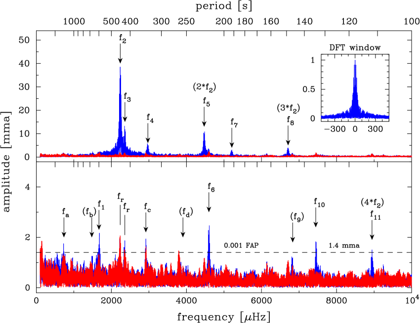
Figure 1: Discrete Fourier transform of the jul11b.ts data set (Jul 27 – Aug 2, 2011). The top panel shows the unmodified DFT (or periodogram) in blue between $10^{2}-10^{4}\mu$ Hz with the vertical scale in millimodulation amplitude (mma) units for which 10 mma represents a 1% modulation of the lightcurve. The DFT after prewhitening by the 6 labelled frequencies is shown in red (lighter shade), and expanded vertically in blue (darker shade) in the bottom panel. The frequencies marked $f_{r}$ correspond to residual power which remained after subtracting $f_{2}$ and $f_{3}$ from the lightcurve and are not considered physical. The four “frequencies” labelled $f_{a}$, $f_{b}$, $f_{c}$, $f_{d}$ represent peaks seen in the DFTs in other runs, but we are reluctant at this stage to confidently identify these as representing real power arising from a pulsation mode. The remaining power after prewhitening by all the identified peaks is again shown in red (lighter shade) in the bottom panel. The frequencies $f_{5}$, $f_{8}$ and $f_{11}$ are clearly harmonics of the 38 mma dominant frequency and have been appropriately co-labelled. (A colour version of this figure is available in the online journal.)

The initial rationale for the development of tsreduce was for the production of real-time lightcurves while observing was in progress. However, improvements made to the code mean that we now use it as part of our final reduction pipeline for our sparse field photometry, as comparisons with other available routines have verified its accuracy. We briefly outline the methodology here.

As mentioned in Section 2.2 the tsreduce software first processes each frame by subtracting a bias level (measured from an overscan region in each frame), subtracting a mean dark frame to remove dark current effects and finally dividing by an appropriate flat field to correct for non-uniform illumination. Synthetic aperture photometry is then performed on the target and (typically two) comparison stars using a central aperture of a fixed radius and a surrounding annular region to estimate the background intensity. The aperture size for the online reduction is determined from the first frame by identifying a minimum aperture radius such that the stellar flux profile is indistinguishable from the background noise level.

The impact of atmospheric effects are minimised by normalising the target light intensity with the sum of the two comparison star intensities, and a low-order polynomial fit is then used to correct for any residual effects such as differential extinction. The developing lightcurves of all three objects, along with the evolving Fourier transform (DFT, see next section) of the target star, are updated in real-time as new frames are acquired during an observing run. The FWHM of the seeing disk is also displayed on a plot as the run proceeds.

Offline analysis routines allow the aperture size to be optimized for the final reduction. In this process we take the pragmatic approach: the user is presented with the corrected lightcurve of the target star, its DFT and the signal-to-noise estimates for different aperture sizes. Thus, an informed decision about the best aperture size can be made. We have yet to find an automated algorithm that can reliably outperform the human eye and brain.

Also, if deemed appropriate, we use the program ts3fix (described in Sullivan et al., 2008) in order to remove obvious lightcurve artifacts such as resdiual transparency variations not corrected for by the polynomial fitting. Futher processing routines convert the time stamps to barycentric Julian days (BJD) and combine multiple runs as appropriate, allowing an analysis to be performed on multiple nights of photometric data.

4 Lightcurve Analysis

4.1 Fourier analysis

Visual inspection of an EC 04207 lightcurve (an example is given in Fig. 2) clearly shows shows a non-sinusoidal oscillation with a period of $\sim 450$ seconds. It is thus no surprise that the Fourier transform (shown in Fig. 1 for the jul11b.ts run) is dominated by a peak at $2236\,\mu$Hz and its harmonics. Formally, in Fig. 1 we have displayed the amplitude power spectrum in which the Fourier transform phase information has been removed; we are only interested in the amplitudes of the sinusoids here. Sometimes this plot is called a periodogram; we will simply call it a DFT (short for discrete Fourier transform). The horizontal plot scale is $\mu$Hz and the vertical plot scale employs millimodulation amplitude (mma) units, for which 10 mma corresponds to a modulation amplitude in the time domain of 1% (which matches the amplitude of a fitted sinusoid of the appropriate frequency and phase).

Table 3: Table of the detected frequencies in the four individual observing runs. The amplitudes are specified in millimodulation amplitude (mma) units and those given in parentheses are below the 0.1% false alarm probability (FAP) for the particular run, but which we believe are likely to be real (see text). The run FAP values are specified in the column headers in square brackets. Frequencies f₁ – f₁₁ labelled by numbered suffixes are well determined across all four observing runs, whereas the four items labelled with letter suffixes a – d exhibit significant power in at least one run, but we consider these only marginal detections of real power. Frequencies deduced to be associated with independent eigenmodes of the star are labelled with a ‘$\star$’.

Item	Frequency	Period	Amplitude [mma]				Assumed
	[$\mu$Hz]	[s]	mar11.ts [2.7]	jul11a.ts [1.5]	jul11b.ts [1.4]	nov11.ts [1.4]	Combinations
fa	736	1358.9	-	-	1.7	1.6	-
fb	1478	676.5	4.1	-	(1.3)	-	-
$\star$f1	1669	599.1	4.7	2.6	1.9	-
$\star$f2	2236	447.2	33.1	38.8	38.4	38.3	-
$\star$f3	2361	423.5	8.7	8.1	8.1	9.2	-
fc	2918	342.7	(1.6)	-	1.7	2.1	-
$\star$f4	2973	336.4	5.8	4.7	5.6	5.1	-
fd	3906	256.0	(2.1)	1.6	-	-	f2 + f1
f5	4473	223.6	7.7	9.0	10.7	10.4	2 f2
f6	4598	217.5	(2.1)	3.2	2.6	2.0	f2 + f3
f7	5209	192.0	2.7	2.1	3.1	2.5	f2 + f4
f8	6709	149.1	2.9	2.8	4.1	4.2	3 f2
f9	6831	146.4	-	(1.4)	(1.3)	1.5	2 f2 + f3
f10	7445	134.3	-	-	1.7	1.4	2 f2 + f4
f11	8945	111.8	-	-	1.4	1.8	4 f2

The window function (Fig. 1, inset) shows the DFT of a noise-free sinusoid sampled at the same times as the observed data. It thus shows the ‘best’ that one can do in visually identifying a frequency from the Fourier transform.

We initially identified real frequencies in the jul11b.ts lightcurve by visual inspection of the DFT. Thus the six frequencies indicated by downward arrows in the top panel of Fig. 1 were selected as real. Given the non-sinusoidal shape of the lightcurve it is clear that we expect to see harmonics of the dominant frequency (f₂) in the DFT. Hence f₅ and f₈ are clearly harmonics of f₂ as their frequency values are exactly two and three times that of f₂, respectively. These are appropriately labelled in Fig. 1.

Identification of real lower amplitude frequencies in a DFT is often complicated by the aliases that arise from significant gaps in the time domain data. This applies here as we have combined multiple nights in our single site observing runs – the frequency resolution is improved but prominent side peaks separated by $11.6\,\mu$Hz (1 day^-1) are also introduced due to the regular gaps with a period of one day. If there are real frequencies in the data with separations comparable to the alias peaks, identification can be difficult.

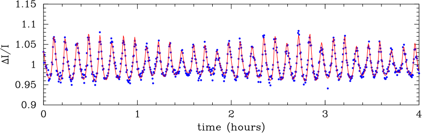
Figure 2: Four hours of a EC 04207 lightcurve that has been fitted by the convection modelling procedure discussed in the paper. The vertical axis depicts the lightcurve modulation in fractional intentity units. The non-sinusoidal pulse shapes in the lightcurve are clearly evident, and the fitting process yielded a value of $\tau_{0}=148\pm 5$ s for the convective response time parameter (see text). (A colour version of this figure is available in the online journal.)

An obvious way to reduce the impact of alias peaks is to obtain more observations during each 24 hour period. This approach led to the formation of the Whole Earth Telescope (WET, Nather et al., 1990), which is a collaboration of observers at multiple sites around the globe with the aim of improving the 24 hour coverage of a particular target over an entire multiple day observing run. EC 04207 was one of the targets during the xcov28 WET run in November 2011. We include here results from the observations obtained at MJUO during xcov28, primarily to show the variation in amplitudes of the modes over our four observing runs. Except for the disappearance and appearance of several small amplitude frequencies, none of the results presented here depend on the overall WET data set.

We have employed the technique of prewhitening to aid us in identifying low level real frequencies in our data sets. Six sinusoids with frequencies corresponding to the large amplitude signals discussed above were least squares fitted for both amplitude and phase to the lightcurve. The resulting model lightcurve was then subtracted from the data. Fixing the frequencies at the DFT derived values allows direct use of the linear least squares procedure. The results can be further optimised by iterating the frequencies using nonlinear least squares techniques, but in practice this makes little difference. Following this procedure, the signal and aliases corresponding to the above frequencies will then have been removed from the DFT of the prewhitened light curve.

This prewhitened DFT is plotted in red (lighter plot) in the top panel of Fig. 1 and is presented in the lower panel using a different vertical scale. The red (lighter) plot in the lower panel represents a DFT further prewhitened by a number of the lower amplitude frequencies.

Using this procedure, fifteen frequencies have been identified, and are presented in Table 4 as well indicated by the labelled downward arrows in Fig. 1.

For the low level signals it is important that noise peaks are not mistaken as real in the DFTs. We have used the false alarm probability (FAP) method, first introduced by Scargle (1982), to quantify this issue. With the speed of modern computers it is now straight forward to employ Monte Carlo methods in this process rather then assume some analytical noise model. To determine the FAP level for a given data set, the time series data is first prewhitened by all of the frequencies with significant amplitudes. This essentially removes the majority of the coherent signal in the data. The timestamps for the resulting measurement values are randomly shuffled, destroying any remaining coherent signal but leaving intact the incoherent noise level. The DFT of the time-shuffled data set is determined and the maximum peak amplitude is recorded. Repeating this exercise N times allows us to use the overall maximum peak value to assert that there is a probablity of 1/N of obtaining a peak in the DFT as high as this value that is due to incoherent noise. It can also be informative to plot a histogram of the collection of maximum values, such as is presented in Sullivan et al. (2008).

We have chosen N to be 1000 and therefore can say that there is a 0.1% chance of a noise “conspiracy” producing a DFT peak as high as the calculated FAP value in each data set. The calculated FAP value (1.4 mma) for the jul11b.ts data set is represented by a dashed line in the bottom panel of Fig. 1, and the mma values for all four data sets are listed in square brackets in the headings in Table 3.

The frequencies we have identified as real at the 99.9% confidence level in the different data sets are listed in Table 3 in terms of their mma values, and marked by downward arrows in Fig. 1 for the jul11b.ts data set. Both in the table and the figure we have used brackets to indicate frequencies that do not strictly meet our FAP criterion but we have other reasons to believe in their reality, such as they correspond to harmonic or sum frequency values or they appear in another data set.

We note that subtracting the large amplitude frequencies, f₂ - f₈, from the July and November runs in some cases left residual power above the 0.1% FAP threshold, particularly for the two largest signals f₂ and f₃. These peaks are labelled by f_r in the bottom panel of Fig. 1.

This residual power was centred between 2 and 6 $\mu$Hz from the subtracted frequency, with several outliers that provided a best fit as far as 50$\mu$Hz away for the DFT of the jul11a.ts data. There does not appear to be any consistent trend in the spacing of these residual peaks between runs, or between frequencies within the same run, so we are not prepared to associate them with physical stellar behaviour. The power may result from instrumental or atmospheric effects in the time domain that we have not properly modelled. The combined data set from the WET run may provide more insights.

The frequencies labelled with letter subscripts, namely $f_{a}$ – $f_{d}$, are really in our uncertain category. Their amplitudes appear in subsets of the four runs above our adopted 0.1% FAP threshhold, but there are reasons to be cautious given their low amplitudes. In particular, $f_{a}$ corresponds to an unusually long period of 1360 s for this class of pulsator and is in the regime where 1/f noise may have an impact on the data. Even though it does appear above the FAP threshhold in two data sets it is perhaps more likely to result from transparency changes.

Taking into account the harmonic and combination frequencies and setting aside the low amplitude ‘frequencies’ $f_{a}$, $f_{b}$ and $f_{c}$, it would appear that EC 04207 is a relatively simple DB pulsator with only four detected pulsation modes, $f_{1}$ – $f_{4}$ (marked with a ‘$\star$’ in Table 3), and with a lightcurve that is dominated by $f_{2}$ (447 s) and its harmonics.

4.2 Nonlinear lightcurve fitting

The Fourier analysis in the previous section clearly indicates that we have only unambiguously identified four independent pulsation modes in EC 04207 from our four photometric data sets. This is not really enough detected eigenmodes of the star for us to place useful constraints on its structure by matching these observed modes with theoretically predicted values. These detected modes could be combined with those observed in other white dwarfs in the same DBV class, and progress made by assuming they have a similar structure – ie employ the techniques of ensemble asteroseismology. Instead we will make use of an asteroseismic tool which focusses on the shape of the observed lightcurve variations that was first introduced by Montgomery (2005).

Building on work first undertaken by Brickhill (1992) and later by Goldreich & Wu (1999) that emphasised the importance of the subsurface convection zones in the white dwarf pulsators, Montgomery (2005) introduced a relatively simple model that enables the extraction of a convection zone parameter from the variations in the lightcurve shapes. In essence Montgomery’s technique models departures of the lightcurve variations from a simple sinusoidal shape with effects introduced by the energy flux transmission through the sub-surface convection zone in the star. The key derived parameter is a time-averaged convective response time $\tau_{0}$, which corresponds to an average time for energy to be trapped and then released by the convection zone by way of the convection mechanism. Montgomery (2005) first sought to model the lightcurves of mono-periodic (or nearly mono-periodic) pulsators, but this was later extended (Montgomery et al., 2010) to include the multiperiodic ones.

The technique assumes that the radiative flux variations occurring at the base of the convection zone are purely sinusoidal and that it is the convective transport process itself that leads to the emergent flux having a nonsinusoidal form. Since the response time is expected to increase with the total mass of the convective layer, the relative times can then be used to differentiate between pulsators with convection zones of various mass and therefore depth. In simple terms, the more nonsinusoidal (“nonlinear”) the measured lightcurve variations, the larger the value of $\tau_{0}$ and therefore the more extended is the convection zone.

The EC 04207 lightcurve variations are clearly non-sinusoidal, as is evident from direct inspection of the lightcurve in Fig. 2 or by viewing the harmonics of the dominant frequency in the DFT in Fig. 1. The first step in the convective lightcurve fitting is to select the independent pulsation modes to be incorporated; the fitting procedure itself introduces harmonics and sum and/or difference frequencies as required in order to match the observed lightcurve. From the amplitudes of the four detected independent pulsation modes displayed in the Fig. 1 DFT, it is clear that f₂ (and its harmonics) along with f₃ and f₄ will explain essentially all of the lightcurve variations. Consequently, these frequencies were chosen for the fit. The parameters for the best fit are given in Table 4.

Table 4: A list of the frequencies of the EC 04207 pulsation modes used in the convection fitting procedure along with the derived parameters. A key result of the lightcurve fitting is the value of $\tau_{0}=148\pm 5$ s for the average convective response time for this star.

Mode	Frequency	Period	Amplitude	$\ell$	m
	[$\mu$Hz]	[s]	[mma]
f2	2236.24	447.18	23.8	1	0
f3	2361.47	423.50	9.8	1	1
f4	2972.66	336.40	4.0	1	0

The solid line in Fig. 2 shows the result of our fitting procedure and it is clear that the model is a good fit to the observed lightcurve and, in particular, it accurately reproduces the non-sinusoidal shape. Table 4 provides a list of parameters describing the three eigenmodes for this best fit, and the time-averaged convective response time for the fit is $\tau_{0}=148\pm 5$ s. Note that the value for $\tau_{0}$ in this fitting procedure is not strongly dependent on the $\ell$ and m values for the eigenmodes used in the fit. Our fitting process also yielded an estimate for the pulsation axis inclination angle of $\theta_{i}=38.8\pm 5$ degrees.

By itself the particular $\tau_{0}$ value is perhaps not that informative, but the comparative values for different pulsators in the instability strip clearly will provide physical insights. In particular, the correlation between the increasing values of $\tau_{0}$ with the decreasing effective temperature estimates for different pulsators looks to be very useful. We discuss this feature in the next section.

5 Discussion

The nonlinear lightcurve fitting procedure has been applied to a number of stars in both the DAV and DBV instability strips, and the correlations between the derived values of $\tau_{0}$ and both the effective temperatures and mean pulsation periods for the different stars have been investigated (Montgomery et al., 2010; Provencal et al., 2012).

The most interesting correlation is the observed increase in the mean convective response time $\tau_{0}$ for a given pulsator versus the decrease in the spectroscopically measured effective temperature. The physical processes underlying this effect appear to be well understood. When a star enters the hot blue edge of the relevant instabilty strip, the convection zone is quite thin and it therefore has only a small impact on the flux variations passing through its layers. As the star cools, this convection zone deepens and becomes more massive, and its effect is to distort the sinudoidal flux variations by introducing increasing nonlinearities; these are modelled in terms of larger $\tau_{0}$ values.

Table 5: The measured convection zone parameter $\tau_{0}$ versus effective temperatures for a selection of DAV pulsators. The values have been taken from Provencal et al. (2012) with some rounding so as to reflect the various uncertainties.

DAV White Dwarf	$\tau_{0}$ [s]	Teff [K]
G 117$-$B15A	30 $\pm$ 10	$12\,000\pm 200$
EC 14012$-$1446	100 $\pm$ 10	$11\,770\pm 25$
G 29$-$38	190 $\pm$ 20	$11\,690\pm 120$
WDJ 1524$-$0030	160 $\pm$ 35	$11\,660\pm 180$
GD 154	1170 $\pm$ 200	$11\,270\pm 170$

The DAV pulsators provide a reasonable empirical test of this model as the instability strip is now well populated and the spectroscopic effective temperature estimates are sufficiently accurate to identify a range of values within it.

In the case of the DBV instability strip there are far fewer known pulsators, but even more importantly the spectroscopic determination of the T_eff values are relatively uncertain, largely due to the lack of sensitivity of the He I lines to changes in temperature in the vicinity of 25 kK (e.g. Bergeron et al., 2011). In addition, small changes in an unknown H contamination in an otherwise pure He atmosphere leads to different inferred T_eff values.

The DBV, EC 04207 being studied in this paper provides an example. The two published spectroscopic measurements of T_eff differ by $\sim$2000 K – 25,000 K (Koester et al., 2001) and 27,300 K (Voss et al., 2007).

Table 6: The measured convection zone parameters $\tau_{0}$ for five DBV white dwarfs in order of the increasing effective temperatures as gauged from the decreasing values of $\tau_{0}$. The $\tau_{0}$ value for PG 1351 is taken from Montgomery (2005) and the values for GD 358 and PG 1654 are from Montgomery et al. (2010). Note that the second entry for GD 358 with the much smaller $\tau_{0}$ = 42 s value corresponds to a surprising temporary change in the lightcurve behaviour of this well studied pulsator, which has been interpreted by Montgomery et al. (2010) as a temporary increase in the star’s T_eff of $\sim 2000$ K.

DBV White Dwarf	$\tau_{0}$ [s]
GD 358	570 $\pm$ 6
EC 04207$-$4748	148 $\pm$ 5
PG 1654$+$160	117 $\pm$ 5
PG 1351$+$489	88 $\pm$ 8
GD 358*	42 $\pm$ 2
EC 20058$-$5234	40 $\pm$ 5

It would appear to be fruitful to use the $\tau_{0}$ values established from the lightcurve fitting process to identify the various pulsators within the DBV instability strip, and then use them to act as a check on the spectroscopic temperatures or even provide an alternative indirect method of establishing their relative temperatures, and therefore their positions within the instability strip.

Montgomery et al. (2010) cite $\tau_{0}$ values extracted from the light curves of the pulsators GD 358, PG 1351+489 and PG 1654+160. We also report here premiminary results for lightcurve analysis of the DBV EC 20058$-$5234 (Sullivan et al., 2007). The lightcurve of this hot white dwarf pulsator exhibits no obvious departures from a sinusoidal form, although there is evidence in the DFTs of small contributions from harmonics and combination frequencies. Using the five dominant pulsation modes (333, 281, 257 333 and 195 [s]) in this star (Sullivan et al., 2008), we have extracted a value of $\tau_{0}\sim 40$ s for EC 20058 from lightcurve fitting.

In Table 6 we have listed these five DBVs in terms of their decreasing numerical values for the deduced average convective response times $\tau_{0}$. This table clearly suggests that EC 20058 with the smallest $\tau_{0}$ value is closest to the blue edge of the DBV instability strip and therefore has the highest T_eff, while the class prototype GD 358 (ie V777) in its normal or quiescent state (Montgomery et al., 2010) with the largest $\tau_{0}$ value is closest to the red edge and has the lowest T_eff.

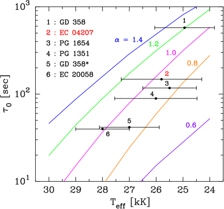
Figure 3: Model convective response times $\tau_{0}$ as a function of T_eff for different values of the $\alpha$ parameter using the ML2 convection model. Note that the measured $\tau_{0}$ value for EC 04027 is broadly consistent with $0.8\leq\alpha\leq 1.2$ using the range of possible T_eff values we have adopted for this star. (A colour version of this figure is available in the online journal.)

In Fig. 3 we have presented expected values for $\tau_{0}$ determined using the ML2 convection model (Böhm & Cassinelli, 1971; Provencal et al., 2012), and plotted these as a function of effective temperature in the vicinity of the DBV instability strip. As is depicted in the figure, we computed model $\tau_{0}$ values for five different values of the ML2 $\alpha$ parameter, which corresponds to the mixing length relative to the atmosphere pressure scale height. The various measured $\tau_{0}$ values for the five DBVs have been added to the plot along with spectroscopically estimated effective temperatures for each star. The T_eff estimates we have used are from the following sources: (1) GD 358 and PG 1351 (Bergeron et al., 2011), (2) EC 04207 and PG 1654 (Voss et al., 2007; Koester et al., 2001) and (3) EC 20058 (D. Koester, private communication). It is important to note that the error bars depicted in Fig. 3 are not really formal uncertainlty estimates, but are in reality indicative intervals for the spectroscopically estimated T_eff values.

Note also that Bergeron et al. (2011) also lists a value for PG 1654 of T${}_{\rm eff}=29\,410\pm 1613$. This appears unreasonably high to us, so either this is a mistake or given the implied range of more than 3 000 K it is very suggestive of the real difficulty of establishing a spectroscopic temperature in the DBV temperature range. In Fig. 3 we have used the lower T_eff published in Voss et al. (2007) along with an appropriate uncertainty estimate.

In a future publication we aim to relate in more detail the measured $\tau_{0}$ values to the spectroscopic measurements of the temperatures.

References

- Althaus et al. (2010) Althaus L. G., Córsico A. H., Isern J., García-Berro E., 2010, A&ARv, 18, 471
- Bergeron et al. (2011) Bergeron P., Wesemael F., Dufour P., Beauchamp A., Hunter C., Saffer R. A., Gianninas A., Ruiz M. T., Limoges M.-M., Dufour P., Fontaine G., Liebert J., 2011, ApJ, 737, 28
- Böhm & Cassinelli (1971) Böhm K. H., Cassinelli J., 1971, aa2, 12, 21B
- Brickhill (1992) Brickhill A. J., 1992, MNRAS, 259, 519
- Fontaine & Brassard (2008) Fontaine G., Brassard P., 2008, PASP, 120, 1043
- Goldreich & Wu (1999) Goldreich P., Wu Y., 1999, ApJ, 511, 904
- Hermes et al. (2012) Hermes J. J., Montgomery M. H., Winget D. E., Brown W. R., Kilic M., Kenyon S. J., 2012, apj2, 750, L28
- Kilkenny et al. (2009) Kilkenny D., O’Donoghue D., Crause L. A., Hambly N., MacGillivray H., 2009, MNRAS, 397, 453
- Koester et al. (2001) Koester D., Napiwotzki R., Christlieb N., Drechsel H., Hagen H.-J., Heber U., Homeier D., Karl C., Leibundgut B., Moehler S., Nelemans G., Pauli E.-M., Reimers D., Renzini A., Yungelson L., 2001, A&A, 378, 556
- Landolt (1968) Landolt A. U., 1968, ApJ, 153, 151
- Montgomery (2005) Montgomery M. H., 2005, ApJ, 633, 1142
- Montgomery et al. (2010) Montgomery M. H., Provencal J. L., Kanaan A., Mukadam A. S., Thompson S. E., Dalessio J., Shipman H. L., Winget D. E., Kepler S. O., Koester D., 2010, ApJ, 716, 84
- Mukadam et al. (2004) Mukadam A. S., Mullally F., Nather R. E., Winget D. E., von Hippel T., Kleinman S. J., Nitta A., Krzesinski J., et al., 2004, ApJ, 607, 982
- Mullally et al. (2006) Mullally S. E., Thompson S. E., Castanheira B. G., Winget D. E., Kepler S. O., Eisenstein D. J., Kleinman S. J., Nitta A., 2006, ApJ, 640, 956
- Nather & Mukadam (2004) Nather R. E., Mukadam A. S., 2004, ApJ, 605, 846
- Nather et al. (1990) Nather R. E., Winget D. E., Clemens J. C., Hansen C. J., Hine B. P., 1990, ApJ, 361, 309
- Nitta et al. (2009) Nitta A., Kleinman S. J., Krzesinski J., Kepler S. O., Metcalfe T. S., Mukadam A. S., Mullally F., Nather R. E., Sullivan D. J., Thompson S. E., Winget D. E., 2009, ApJ, 690, 560
- Østensen et al. (2011) Østensen R. H., Bloemen S., Vučković M., Aerts C., Oreiro R., Kinemuchi K., Still M., Koester D., 2011, apj2, 736, L39
- Provencal et al. (2012) Provencal J. L., et al., 2012, ApJ, 751, 91
- Scargle (1982) Scargle J. D., 1982, ApJ, 263, 835
- Stobie et al. (1997) Stobie R. S., Kilkenny D., O’Donoghue D., Chen A., Koen C., Morgan D. H., Barrow J., Buckley D A. H., Cannon R. D., Cass C. J. P., et al., 1997, MNRAS, 287, 848
- Sullivan (2000) Sullivan D. J., 2000, Baltic Astronomy, 9, 425
- Sullivan et al. (2008) Sullivan D. J., et al., 2008, MNRAS, 387, 137
- Sullivan et al. (2007) Sullivan D. J., Metcalfe T., O’Donoghue D., Winget D. E., et al., 2007, in Napiwotzki R., Burleigh M., eds, 15th European Workshop on White Dwarfs Vol. 372 of ASP Conf.. Astron. Soc. Pac., San Francisco, p. 629
- Voss et al. (2007) Voss B., Koester D., Napiwotzki R., Christlieb N., Reimers D., 2007, A&A, 470, 1079
- Winget & Kepler (2008) Winget D. E., Kepler S. O., 2008, Ann.Rev.Astron.Ap., 46, 157
- Winget et al. (1982) Winget D. E., Robinson E. L., Nather R. E., Fontaine G., 1982, ApJ, 262, L11