Astronomy below the Survey Threshold

Abstract:

Astronomy at or below the survey threshold has expanded significantly since the publication of the original Science with the Square Kilometer Array in 1999 and its update in 2004. The techniques in this regime may be broadly (but far from exclusively) defined as confusion or P(D) analyses (analyses of one-point statistics), and stacking, accounting for the flux-density distribution of noise-limited images co-added at the positions of objects detected/isolated in a different waveband. Here we discuss the relevant issues, present some examples of recent analyses, and consider some of the consequences for the design and use of surveys with the SKA and its pathfinders.

1 Astronomy beneath the Survey Threshold

Since the publication of the original SKA science case (Taylor & Braun, 1999), and indeed since the 2004 publication of its update by Carilli & Rawlings, more has been understood about sub-threshold astronomy and numerous detailed analyses have shown how to extract astronomical and cosmological results. We look to summarize these developments, issues and techniques, as well as to note some implications for the SKA, its precursors and pathfinders. We largely restrict our discussion to the radio continuum, while noting that sub-threshold techniques are highly applicable (a) to other wavebands (e.g. Marsden et al. 2009, Bourne et al. 2012), (b) when using polarization to investigate cosmic magnetism (Stil 2015), and (c) for HI spectral-line work (Blyth et al. 2015).

Source surface densities generally rise steeply with decreasing source intensity — i.e. the source count is ‘steep’. With this come two aspects of surveys now generally accepted. Firstly, it is very unwise to ‘push’ cataloguing and source-counting — the survey threshold — down to anywhere near the confusion limit or the noise limit; the combined effects of these plus Eddington bias require cataloguing to be limited to intensities ¿ 5$\sigma$, $\sigma$ representing the combined confusion (see below) and system noise. Second, there is much astronomy to be done with proper and rigorous statistical interpretation of survey data to levels well below this threshold.

Confusion analysis (P(D), or single-point statistics) as first proposed by Scheuer (1957) is essentially single-frequency, extending our knowledge of the source count at that frequency to intensities below the threshold. Stacking on the other hand was a conscious product of multi-waveband astronomy, to investigate bulk properties of objects above thresholds and in catalogues in one waveband, but generally (not exclusively) below survey thresholds in another band. Stacking then implies adding images in the latter band at the positions of the catalogue in the former, to discover average faint intensities. It was perhaps pioneered in the X-ray regime (Caillault & Helfand 1985) for the average X-ray properties of G-stars. By the time of the SDSS survey, sophisticated analyses were carried out to examine radio properties of radio-quiet quasars (White et al., 2007), and indeed radio-quiet galaxies (Hodge et al., 2008). Chief requirements are absolute astrometry to better than 1 arcsec in both bands and good dynamic range in the sub-threshold band.

It is essential for galaxy-formation and evolution studies to be able to investigate both faint AGN and star-formation activity (see e.g. Smolčić et al. 2008, 2009a, 2009b; Seymour et al. 2009; Bonzini et al. 2013; Padovani et al. 2014). This is particularly so in view of the now commonly accepted link between an AGN phase and the quenching of star formation (Begelman 2004; Croton et al. 2006) in order to effect cosmic downsizing. In addition, the statistical techniques discussed here bring within reach a wealth of extragalactic astrophysics considered further in Jarvis et al. (2015); Kapinska et al. (2015); McAlpine et al. (2015); Murphy et al. (2015); Smolčić et al. (2015). These make it possible to proceed from noisy flux measurements to source counts, luminosity functions, star-formation rates and their cosmic densities, all as a function of e.g. environment, stellar mass, redshift, but only when ancillary data are available. More comprehensive introductions to the science available via stacking and $P(D)$ analyses (together with comprehensive referencing) are provided in Glenn et al. (2010); Padovani (2011); Heywood et al. (2013); Zwart et al. (2014).

2 Beating the Survey Threshold

Before describing the methods of $P(D)$ and stacking — and their biases — in more detail, we set out some relevant definitions. Confusion and associated concepts are discussed in the following points, and these may be clearer on examination of Figs 1 and 2.

• Confusion is integration or blending of the background of faint sources by either (a) the finite synthesized beam (spatial response) of a telescope, or (b) the intrinsic angular extents of the sources. The anisotropies of blended background sources become visible when instrumental noise is low enough.

• Intrinsic (Natural) Confusion, also sometimes referred to as Source Blending (which has still other meanings), occurs if extended sources/objects in any image — at any wavelength — physically overlap on the sky. Note that this is independent of the resolution of the image, as it depends only on the intrinsic (distribution, angular-diameter and density) properties of the sources. For 1.4-GHz radio surveys, intrinsic confusion occurs at well below 1-$\mu$Jy rms (Windhorst, 2003).

• Instrumental Confusion occurs if the source density is so high that sources are likely to be detected in a ‘significant’ fraction of the resolution elements (PSFs/synthezised beams) in an image. This is the most commonly assumed form of confusion and it generally comes to mind when the term is used.

• Sidelobe Confusion happens if bright sources are likely to appear in the sidelobes of the synthesized beam to the extent that the Dynamic Range of the image is compromised (Makhathini et al. 2015; Smirnov et al. in prep.).

• Identification Confusion occurs when the combination of resolution and positional accuracy in the radio image and the density of sources at a cross-identification wavelength (e.g. optical or infra-red), are such that a ‘significant’ fraction of the sources cannot be reliably identified with objects seen at the other wavelength. The likelihood ratio is an example of a method that can be used to overcome this (see e.g. McAlpine et al. 2012).

• Confusion Limit There are various meanings. If used in the context of surveys for discrete sources, the term is sometimes used to signify the flux-density depth to which discrete sources can be reliably detected and their intensities measured. In the foregoing we have referred to this as the survey threshold. At the brighter end of the source count with steep slope of about $-$2.7, a safe threshold is the flux density at which the surface density is perhaps 50 beam-areas per source; at faint flux densities where the count slope is less steep, say $-$1.7, it becomes $\approx$25 beam-areas per source (Condon, 2013). The confusion limit, the level at which the background is totally blended as depicted in Fig. 1, must occur at flux densities corresponding to source densities of $>$ one source per beam area. The confusion limit is also taken at times to mean the flux density at which the confusion noise is equal to system noise.

• Confusion Noise is generally taken to be a single-point statistic describing the width of the distribution of single pixel values in a confusion-dominated image; see Figs 1 and 2. The origin of this ‘noise’ depends on which type of confusion is in question. Since the single-point distribution is usually highly skewed and very non-Gaussian (Condon, 2013), a single descriptor of it is not suitable. Theoretically the distribution for a power-law source count has an infinite tail to the positive side so that the mean and variance are infinite. (With very ‘steep’ counts approaching $-$3 in slope, the distribution does approximate Gaussian.) ‘Shallow’ slopes result in a preponderance of brighter source intensities and a long positive tail. Despite the dangers, some approximation to the core width is generally made to compare with system noise or in rough calculations of attainable survey depth. Under some circumstances (e.g. Feroz et al. 2009) an estimate of the confusion noise per beam is taken to be the second moment of the residual differential source count up to some limiting threshold, where all sources with flux densities greater than that threshold have already been subtracted; one feature of/problem with this definition is that confusion noise is then a sensitive function of survey noise i.e. integration time. Fig. 3 shows a way to scale the instrumental confusion to different resolutions and/or frequencies near 1.4 GHz (see also Condon et al. 2012).

• Eddington bias is the apparent steepening of the observed source count (Eddington, 1913) by the intensity-dependent over-estimation of intensities, due to either system noise or confusion noise or both. The process of over-estimating flux densities of faint sources is sometimes called flux boosting, a misleading term because no physical increase of observed intensity is taking place, as it is in the case of relativistic beaming. Jauncey (1968) first drew ‘flux boosting’ to our attention; it was the submm astronomers who identified it as leading to Eddington bias and grasped how to estimate unbiased flux densities (and hence counts) using a Bayesian Likelihood Analysis (BLA) and count estimates as priors (Wall & Jenkins 2003; Coppin et al. 2005).

• Estimators and biases Flux densities measured by standard techniques, e.g. PSF fitting, or average pixel value near a map peak, are not flux densities, but like all measured quantities, are estimators of flux densities. If instrumental or confusion noise is significant and the source count strongly favours faint intensities, the usual case, then such an estimator will be biased. The flux density is not boosted — the measurement is wrong. De-biasing, deboosting or however it is termed, is simply stating that a better — possibly even unbiased — estimator is being used.

• Probability of deflection, P(D), or P(D) distribution, is the full distribution of single-pixel values. P(D) analysis is the analysis of this distribution (see Section 2.1) to deduce the underlying faint source count.

• Stacking (Section 2.2) is the co-addition of maps at the positions of sources detected in another map or catalogue. In contrast to a $P(D)$ blind analysis, stacking is intrinsically prior-based source extraction, but can also be used to conquer confusion.

Figure 1: A 3-GHz image from a 57-hour integration with the Karl G. Jansky Very Large Array (VLA) in C-configuration (Condon et al., 2012), with synthesized beam 8-arcsec FWHM. The instrumental noise is 1.02 $\mu$Jy beam^-1. All features in the image, positive and negative, are on beamwidth scales and these cover the image, indicating that the background of faint sources has been completely smoothed or integrated by the beam response. The large positive deflections represent discrete radio sources, producing the long positive tail of the $P(D)$ distribution (Condon et al. 2012; Vernstrom et al. 2014b; see Fig. 2).

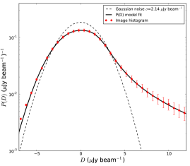
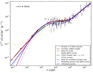
Figure 2: Left — Oversampled P(D) distribution (Vernstrom et al., 2014b) for the central 5-arcmin radius of the 3-GHz image of Fig. 1 (dots and $\sqrt{N}$ error bars), with the best-fitting 8-node model (solid curve). The dashed line represents a Gaussian of $\sigma=$1.255 $\mu$Jy, accurately describing the instrumental noise. Right — Source counts at 1.4 GHz, shown in relative differential form. Points and error bars show previous estimates of the counts from the literature. The short straight (green) line plus dashed lines above and below it show results from Condon et al. (2012), the early interpretation of the current deep survey data. Joined points plus dashed error limits show the results from the $P(D)$ analysis of Vernstrom et al. (2014b), translated from 3.0 to 1.4 GHz with a spectral index of $-$0.7. Smooth curves represent counts calculated from models of radio and infra-red luminosity functions and cosmic evolution; see Vernstrom et al. (2014b) for references.

Figure 3: 1.4-GHz ‘rms’ confusion $\sigma$ for point sources based on the Wilman et al. (2008) source count, as a function of FWHM resolution for a Gaussian beam in units of Jy beam^-1 and K of brightness temperature. The ‘rms’ is defined in this diagram as half the Jy beam^-1 or K range containing two thirds of the data points, making it a more stable statistic given the long tails of the $P(D)$ distribution. The curves can be rescaled to nearby frequencies by scaling $\sigma_{\mathrm{S}}\propto\nu^{-0.7}$ or $\sigma_{\mathrm{T}}\propto\nu^{-2.7}$.

We now discuss strategies for analysing noise-limited data, be they confusion-limited or system-noise limited. The two prevailing techniques, which are complementary, are either blind ($P(D)$ analysis) or prior-based (stacking).

2.1 Probability of Deflection (P(D)) analysis

The technique was first applied by Hewish (1961) to estimate counts at 178 MHz by forward modelling, using the 4C survey data. P(D) has been adopted to estimate source counts (with subsequent constraints on luminosity functions) at a number of wavebands other than radio, e.g. X-ray (Toffolatti & Barcons, 1992; Barcons et al., 1994); infra-red (Jenkins & Reid, 1991; Oliver et al., 1992); far infra-red (Friedmann et al., 2002); and submm (Patanchon et al., 2009). Most recently (Vernstrom et al., 2014b) it has been applied to the confusion-limited data of the VLA single-pointing Condon et al. (2012) integration (Fig. 1). A Bayesian Likelihood Analysis was used, with a multi-node count model (Patanchon et al., 2009). The results are in Fig. 2, which demonstrates how the P(D) analysis has resolved the discrepant direct counts and has extended knowledge of the 3-GHz count to nanoJy levels.

$P(D)$ analysis in the face of extended source structures is highly problematic. P(D) analyses to date have assumed no effects of resolution, i.e. assume source angular sizes ¡¡ beam sizes. It is possible to attempt such analyses on the basis of (risky) asumptions about angular structures. A different approach was adopted by Vernstrom et al. (2014a). Their analysis of ATCA data at 1.75 GHz obtained with a $\approx$ 1-arcmin beam suggested an excess of diffuse emission on scales of 1–2 arcmin. To carry out a correct $P(D)$ analysis in the face of source resolution generally requires detailed knowledge of the angular-size distribution of sources as a function of faint flux density. For example, SKA1 surveys could be used to deduce the angular-size distribution, which could then be extrapolated to fainter levels to aid the $P(D)$ analysis. But any population for which we had such detailed knowledge would probably not require data from $P(D)$ analyses. Moreover any tacit assumption that we ‘know’ the composition of the faint-source populations to be star-forming, and that therefore we can infer faint radio-source structures from optical data, is premature.

2.2 Stacking

The literature is very ambiguous on the precise definition of stacking, perhaps the most succinct being “taking the covariance of a map with a catalogue” (Marsden et al., 2009). Having made some selection of sources in an often-deeper (in terms of raw surface density) catalogue, one measures the flux in a map, usually at another wavelength, building up a distribution of map-extracted fluxes for that sample. For example, one might select sources in the near infra-red (i.e. by stellar mass; e.g. Dunne et al. 2009; Karim et al. 2011; Zwart et al. 2014) and measure their 1.4-GHz fluxes, using photometric redshifts to convert those fluxes into star-formation rates via calibration to the far-infra-red–radio correlation (e.g. Yun et al. 2001; Condon et al. 2002). Or one might stack a total-intensity catalogue in polarization in order to investigate cosmic magnetism (Stil, 2015). The flux histogram thus obtained resembles the $P(D)$ of Fig. 2 (left-hand dotted line), and can be binned by some physical quantity, e.g. stellar mass and/or redshift.

Sufficiently rich surveys (with respect to areal coverage/depth) to-date routinely beat individual detection/confusion limits by an order of magnitude to recover the average (see below) properties of pre-selected source populations. The main complications arise if the angular resolution of the map to be stacked is much coarser than in the selection band. For coarse-resolution maps, signal from more than one source can contribute to the net flux in a given pixel in the stacking band (e.g. Webb et al. 2004, Greve et al. 2010) and due consideration must be given to this as a possible source of confusion noise. However, similar problems can in principle arise even at high angular resolution as the source density increases for deeper maps. One might hence conclude that a stacking experiment suffers under low-angular-resolution conditions as well as when survey sensitivity is increasing. The effects of source crowding are negligible if the source distribution is random, following a Poisson distribution at least at the scale of the beam (Marsden et al. 2009; Viero et al. 2012). Even if the latter condition were violated, efficient deblending algorithms have been proposed (e.g. Kurczynski & Gawiser 2010).

Which average? A key difficulty (see e.g. White et al. 2007) is what summary statistic to use to describe the flux distribution (as a whole or within each bin), if any. Since the brightest discrete sources generate a long tail to higher fluxes, the median is generally preferred over the mean. But there are a number of biases that can corrupt this estimator, including the flux limits and shape of the underlying intrinsic (to the population) distribution, as well as the magnitude of the map noise (Bourne et al., 2012). Indeed, much current work is focussed on the identification and elimination of sources of bias, and even circumventing entirely the difficult need for debiasing a single summary statistic.

One promising avenue is the development of algorithms for modelling the underlying source-count distribution (or other/intrinsic physical property) parametrically in the presence of measurement noise (see e.g. Condon et al. 2013), without the use of a single (usually biased) summary statistic. Mitchell-Wynne et al. (2014) demonstrated such a technique on a COSMOS catalogue and FIRST maps, recovering the COSMOS source counts correctly from the FIRST data using a Maximum-Likelihood method to reach $0.75\sigma$ with 500 sources.

Zwart et al. (in prep.) have extended this work to a fully-Bayesian framework, allowing model selection through the Bayesian evidence, to measure 1.4-GHz source counts for a near-infrared-selected sample. Early indications are that the survey threshold can be beaten by up to two orders of magnitude. Roseboom & Best (2014) also used a BLA to measure luminosity functions, as a function of redshift, right from stacked fluxes. And Johnston, Smith and Zwart (in prep.) are incorporating redshift evolution directly into the modelling process. We also note another stacking technique (Lindroos & Knudsen 2013; Lindroos et al. 2014; Knudsen et al. 2015) in which visibilities are calculated at the positions of known sources and then co-added, with the advantage over an image-plane analysis that it leads to reduced uncertainties.

Finally, stacking and $P(D)$ can take a role in the handling of systematics. For example, in the 1–5$\sigma$ regime, P(D) has a strong signal in terms of the source count at least, and if nothing else, P(D) source-count analyses can show just what and when Eddington bias overwhelms the data, so that one can decide a posteriori whether to count discrete sources down to 6$\sigma$ or 3.2$\sigma$ (or at whichever threshold is suitable). It has played its part in the characterization of CLEAN bias in FIRST (see e.g. Stil 2015). Seymour (in prep.) has proposed stacking independent interferometer pointings in order to obtain the primary beam and total noise.

3 The Road to SKA

There are a number of systematics in $P(D)$ and stacking experiments that must be understood during the analysis of pathfinder data. Here we give a summary of the dominant systematics relevant to the sub-threshold regime about which we currently know.

1. CLEAN/snapshot bias; this pernicious effect occurs where instantaneous uv coverage is limited. This could therefore be a concern for wide-field snapshot surveys, but less of a problem for longer-integration targeted deep fields such as those envisaged for SKA1-MID. White et al. (2007) were able to correct for the bias with a simple scaling factor, appearing to be linear even to relatively faint flux densities.

2. Resolution bias; Stil et al. (2014) pointed out that a bias is introduced when the synthesized beam is undersampled. So for stacking SKA1 data, one may require higher-resolution images than allowed for by simply requiring the synthesized beam to be Nyquist-sampled. One must give due consideration to astrometry.

3. Instrumental calibration, e.g. primary beam model, will certainly be an issue for SKA1; as a sky-based phenomenon, characterization of the primary beam is critical for noise-regime analyses, especially as one wants to go to larger areas and/or mosaics and for polarization. Another example is time-dependent system temperatures (corresponding to spatially-varying map noise) for e.g. VLBI. Joint solution of sky and systematics is beginning to be investigated (Lochner et al., in prep.) but is not routine. See also Smirnov et al. (in prep.).

4. Sidelobe confusion (as opposed to classical confusion), is additional noise introduced into an image via imperfect source deconvolution within the image (i.e. by all sources below the source subtraction cut-off limit) and from the (asymmetric) array response to sources outside the imaged field-of-view. Grobler et al. (2014) give an example of artifacts buried in the thermal noise. For instruments with a large field-of-view this is particularly challenging and the instrumental artifacts are hard to separate from classical confusion. This is where an accurate $P(D)$ and careful stacking analyses (section 2.2) will couple to fully exploit the imaging of the SKA surveys.

5. Noise characterization is an issue for any survey; understanding of the noise structure is critical for obtaining the correct result in a $P(D)$ or stacking experiment. Uncertainties on source intensities could vary by position in the map (e.g. the mosaicking eggbox sensitivity pattern), by depth (if the confusion noise begins to contribute in a stacking experiment, or if the dirty synthesized beam begins to enter the stack), or by resolution (confusion noise again). If one has some idea of the functional form of the noise, it can be fitted simultaneously with the physics quantities; debiasing a single-point average is rather harder. In a fully Bayesian analysis the likelihood function should be appropriate for the distribution of the measurement uncertainties.

6. Source clustering and sample variance, which Heywood et al. (2013) showed how to limit in the survey-design phase. This has also been tackled in the submillimetre by Viero et al. (2013).

7. Simulations are of crucial importance to all these analyses (for estimating biases due to clustering to give but one example). For radio-continuum studies we use the work of Wilman et al. (2008). Note that accounting for the (possible) background excess found by ARCADE2 (Fixsen et al., 2011) may require new sub-$\mu$Jy populations (Seiffert et al., 2011; Vernstrom et al., 2011, 2014b). These in turn would require simulations differing from those available via the Wilman et al. prescription, not yet formulated as we move into the pathfinder phase.

The SKA pathfinders such as LOFAR, MWA, MeerKAT and ASKAP themselves will clearly play a key role both in allowing us to update our source-count constraints, as well as in improving statistical techniques that in turn can be adopted for SKA1 analyses, to which we now turn our attention.

4 Considerations for SKA

The integrated version of the count (Vernstrom et al., 2014a) provides important source-surface-density data for design of SKA pathfinder surveys and for development of the SKA. However, extrapolation to other survey wavelengths via a single spectral index must be restricted to a factor of 2 at most, to say 1.4 and 5.0 GHz, and even then over only a limited flux-density range. Counts outside this frequency range differ markedly, and these differences have been modelled by radio-source population syntheses, e.g. Jackson & Wall (1999); Wilman et al. (2008); Massardi et al. (2011).

While it would be speculatory at this stage to predict the confusion implications for the full SKA, various authors have made calculations for SKA1, including present authors, Prandoni & Seymour (2015), and Condon (2013). Illustrative calculations are shown in Figs 4 and 5 (for details of the reference surveys refer to Prandoni & Seymour 2015). Although the details remain to be calculated in the light of the newest deep count estimates (e.g. Vernstrom et al. 2014a, b), general statements can be made. We deal with SKA1-LOW then SKA1-MID/SUR.

Firstly, $P(D)$ experiments at full sensitivity are only anticipated for the lowest frequencies and possibly in the deepest fields, where SKA1(-LOW) will see true confusion-limited data. The SKA will be limited by dynamic range (see section 2), and maximizing this will require care in configuration design (Condon, 2013). Second, SKA1-LOW will obtain its confusion-limited data easily so that (a) survey design needs much consideration and (b) confusion or $P(D)$ experiments will be possible. These experiments may be of great significance, because of the unknown contribution of very steep-spectrum populations favoured at low frequencies. Such sources are hard to detect at faint intensities/large distances of $\approx$1.4-GHz surveys because of $K$-corrections. Their presence or otherwise in the low-frequency source count will be telling in terms of their presumed epoch-dependent luminosity function. Likewise there is likely to be unique potential to probe star-forming galaxies to higher redshifts than has previously been possible.

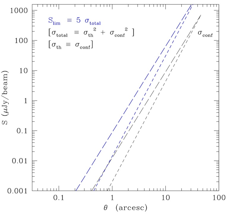
Figure 4: 1.4-GHz limits (dashed and dotted blue lines) of confusion-limited surveys, as a function of spatial resolution $\theta=$ HPBW. Two estimates of the confusion noise are considered. The first (dashed line) is the classical formulation, assuming the source counts derived by Condon et al. (2012), i.e. $N(S)\approx 9000S^{-1.7}$ Jy sr^-1 at 3 GHz translating to $N(S)\approx 12000S^{-1.7}$ Jy sr^-1 at 1.4 GHz. The second (dotted line) uses the approximation of Eq. 27 of Condon et al. (2012) assuming $\nu=1.4$ GHz.

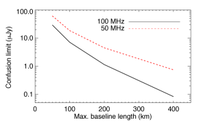
Figure 5: Left – the 1-$\sigma$ flux density at which the survey threshold/confusion limit (here taken as depth at which there is one $>3\sigma$ source per 20 beams) is reached for increasing maximum baseline. Right – integration time per pointing needed to reach this limit for increasing maximum baseline. A maximum baseline of $>100$ km is needed for surveys deeper than 10 $\mu$Jy.

Estimates for the SKA1-LOW classical-confusion limit extrapolate higher-frequency source counts (e.g. 1.4 GHz) because of the paucity of deep $\approx$150-MHz source-count data. While there is a steep slope across the $\approx$100 mJy–1 Jy 150-MHz differential source count, this will flatten if there is a sizeable, fainter source population at $S_{150\,\mathrm{MHz}}<10\,$mJy. This behaviour is predicted by the flattening of the 1.4-GHz differential source count at $S_{1.4\,\mathrm{GHz}}\lesssim 2\,$mJy. Previous work, which has adopted a standard spectral index to extrapolate from 1.4 GHz to 150 MHz in order to predict the low-frequency sky, could be naïve: it assumes that the fainter population observed at 1.4 GHz obeys a standard spectral index ($\alpha=-0.7$) and/or that there is no low frequency (only) very steep-spectrum faint population that is undetectable at 1.4 GHz.

For SKA1-MID, survey design needs careful consideration in terms of whether confusion is to be avoided, or whether it is the object of experiment (i.e. $P(D)$). The detection thresholds of SKA1-MID/SUR will be vastly lower than those of SKA1-LOW, mainly allowing for stacking probes of radio populations selected in the formers’ higher-frequency all-sky surveys. But ultra-deep probes will demand an adequate handling of source-clustering biases despite the high angular resolutions the SKA will achieve at typical (GHz) survey wavelengths.

On the subject of panchromatic data, it is anticipated that stacking will be undertaken in both wide and deep surveys, and Euclid and LSST will almost certainly play a role here (Bourke et al., 2015). If millions of sources are detected by EUCLID, for example, over a wide redshift range, and only (say) 20 per cent are directly detected in the radio, then stacking SKA1-MID data allows for the potential to capture a substantial fraction of the galaxy population in order to measure the luminosity functions of star-forming and AGN galaxies, and as a function of environment (see elsewhere in this volume).

Characterization of any SKA1-MID-detected diffuse emission (such as cluster halos and relics) that couples to shorter baselines will necessarily require a good understanding of confusion noise (see e.g. Feroz et al. 2009). Stacking itself is highly applicable for detecting such emission and constraining scaling relations (e.g. Sehgal et al. 2013).

References

- Barcons et al. (1994) Barcons, X., Raymont, G. B., Warwick, R. S., et al. 1994, Mon. Not. R. Astr. Soc., 268, 833
- Begelman (2004) Begelman, M. C. 2004, in Coevolution of Black Holes and Galaxies, 374
- Blyth et al. (2015) Blyth, S., et al. 2015, in Proceedings of “Advancing Astrophysics with the Square Kilometre Array”, \posPoS(AASKA14)128
- Bonzini et al. (2013) Bonzini, M., Padovani, P., Mainieri, V., et al. 2013, Mon. Not. R. Astr. Soc., 436, 3759
- Bourke et al. (2015) Bourke, T., et al. 2015, in Proceedings of “Advancing Astrophysics with the Square Kilometre Array”, \posPoS(AASKA14)164
- Bourne et al. (2012) Bourne, N., et al. 2012, Mon. Not. R. Astr. Soc., 421, 3027
- Caillault & Helfand (1985) Caillault, J.-P., & Helfand, D. J. 1985, Astrophys. J., 289, 279
- Carilli & Rawlings (2004) Carilli, C. L., & Rawlings, S. 2004, New Astronomy Reviews, 48, 979
- Condon (2013) Condon, J. 2013, Requirements for Continuum Surveys with SKA1, Tech. rep., NRAO
- Condon et al. (2002) Condon, J. J., Cotton, W. D., & Broderick, J. J. 2002, Astron. J., 124, 675
- Condon et al. (2013) Condon, J. J., Kellermann, K. I., Kimball, A. E., Ivezić, Ž., & Perley, R. A. 2013, Astrophys. J., 768, 37
- Condon et al. (2012) Condon, J. J., Cotton, W. D., Fomalont, E. B., et al. 2012, Astrophys. J., 758, 23
- Coppin et al. (2005) Coppin, K., Halpern, M., Scott, D., Borys, C., & Chapman, S. 2005, Mon. Not. R. Astr. Soc., 357, 1022
- Croton et al. (2006) Croton, D. J., Springel, V., White, S. D. M., et al. 2006, Mon. Not. R. Astr. Soc., 365, 11
- Dunne et al. (2009) Dunne, L., Ivison, R. J., Maddox, S., et al. 2009, Mon. Not. R. Astr. Soc., 394, 3
- Eddington (1913) Eddington, A. S. 1913, Mon. Not. R. Astr. Soc., 73, 359
- Feroz et al. (2009) Feroz, F., Hobson, M. P., Zwart, J. T. L., Saunders, R. D. E., & Grainge, K. J. B. 2009, Mon. Not. R. Astr. Soc., 398, 2049
- Fixsen et al. (2011) Fixsen, D. J., Kogut, A., Levin, S., et al. 2011, Astrophys. J., 734, 5
- Friedmann et al. (2002) Friedmann, Y., Bouchet, F., Blaizot, J., & Lagache, G. 2002, in EAS Publications Series, Vol. 4, EAS Publications Series, ed. M. Giard, J. P. Bernard, A. Klotz, & I. Ristorcelli, 357–357
- Glenn et al. (2010) Glenn, J., Conley, A., Bethermin, M., et al. 2010, Mon. Not. R. Astr. Soc., 409, 109
- Greve et al. (2010) Greve, T. R., et al. 2010, Astrophys. J., 719, 483
- Grobler et al. (2014) Grobler, T. L., Nunhokee, C. D., Smirnov, O. M., van Zyl, A. J., & de Bruyn, A. G. 2014, Mon. Not. R. Astr. Soc., 439, 4030
- Hewish (1961) Hewish, A. 1961, Mon. Not. R. Astr. Soc., 123, 167
- Heywood et al. (2013) Heywood, I., Jarvis, M. J., & Condon, J. J. 2013, Mon. Not. R. Astr. Soc., 432, 2625
- Hodge et al. (2008) Hodge, J. A., Becker, R. H., White, R. L., & de Vries, W. H. 2008, Astron. J., 136, 1097
- Jackson & Wall (1999) Jackson, C. A., & Wall, J. V. 1999, Mon. Not. R. Astr. Soc., 304, 160
- Jarvis et al. (2015) Jarvis, M. J., et al. 2015, in Proceedings of “Advancing Astrophysics with the Square Kilometre Array”, \posPoS(AASKA14)068
- Jauncey (1968) Jauncey, D. L. 1968, Astrophys. J., 152, 647
- Jenkins & Reid (1991) Jenkins, C. R., & Reid, I. N. 1991, Astron. J., 101, 1595
- Kapinska et al. (2015) Kapinska, A., et al. 2015, in Proceedings of “Advancing Astrophysics with the Square Kilometre Array”, \posPoS(AASKA14)173
- Karim et al. (2011) Karim, A., Schinnerer, E., Martínez-Sansigre, A., et al. 2011, Astrophys. J., 730, 61
- Knudsen et al. (2015) Knudsen, K. K., et al. 2015, in Proceedings of “Advancing Astrophysics with the Square Kilometre Array”, \posPoS(AASKA14)168
- Kurczynski & Gawiser (2010) Kurczynski, P., & Gawiser, E. 2010, Astron. J., 139, 1592
- Lindroos & Knudsen (2013) Lindroos, L., & Knudsen, K. K. 2013, in IAU Symposium, Vol. 295, IAU Symposium, ed. D. Thomas, A. Pasquali, & I. Ferreras, 94–94
- Lindroos et al. (2014) Lindroos, L., Knudsen, K. K., Vlemmings, W., Conway, J., & Martí-Vidal, I. 2014, ArXiv e-prints, arXiv:1411.1410
- Makhathini et al. (2015) Makhathini, S., et al. 2015, in Proceedings of “Advancing Astrophysics with the Square Kilometre Array”, \posPoS(AASKA14)081
- Marsden et al. (2009) Marsden, G., et al. 2009, Astrophys. J., 707, 1729
- Massardi et al. (2011) Massardi, M., et al. 2011, Mon. Not. R. Astr. Soc., 412, 318
- McAlpine et al. (2012) McAlpine, K., Smith, D. J. B., Jarvis, M. J., Bonfield, D. G., & Fleuren, S. 2012, Mon. Not. R. Astr. Soc., 423, 132
- McAlpine et al. (2015) McAlpine, K., et al. 2015, in Proceedings of “Advancing Astrophysics with the Square Kilometre Array”, \posPoS(AASKA14)083
- Mitchell-Wynne et al. (2014) Mitchell-Wynne, K., Santos, M. G., Afonso, J., & Jarvis, M. J. 2014, Mon. Not. R. Astr. Soc., 437, 2270
- Murphy et al. (2015) Murphy, E., et al. 2015, in Proceedings of “Advancing Astrophysics with the Square Kilometre Array”, \posPoS(AASKA14)085
- Oliver et al. (1992) Oliver, S. J., Rowan-Robinson, M., & Saunders, W. 1992, Mon. Not. R. Astr. Soc., 256, 15P
- Padovani (2011) Padovani, P. 2011, Mon. Not. R. Astr. Soc., 411, 1547
- Padovani et al. (2014) Padovani, P., Bonzini, M., Miller, N., et al. 2014, in IAU Symposium, Vol. 304, IAU Symposium, 79–85
- Patanchon et al. (2009) Patanchon, G., Ade, P. A. R., Bock, J. J., et al. 2009, Astrophys. J., 707, 1750
- Prandoni & Seymour (2015) Prandoni, I., & Seymour, N. 2015, in Proceedings of “Advancing Astrophysics with the Square Kilometre Array”, \posPoS(AASKA14)067
- Roseboom & Best (2014) Roseboom, I. G., & Best, P. N. 2014, Mon. Not. R. Astr. Soc., 439, 1286
- Scheuer (1957) Scheuer, P. A. G. 1957, Proc. Camb. Phil. Soc., 53, 764
- Sehgal et al. (2013) Sehgal, N., et al. 2013, Astrophys. J., 767, 38
- Seiffert et al. (2011) Seiffert, M., Fixsen, D. J., Kogut, A., et al. 2011, Astrophys. J., 734, 6
- Seymour et al. (2009) Seymour, N., Huynh, M., Dwelly, T., et al. 2009, Mon. Not. R. Astr. Soc., 398, 1573
- Smolčić et al. (2008) Smolčić, V., Schinnerer, E., Scodeggio, M., et al. 2008, Astophys. J. Suppl., 177, 14
- Smolčić et al. (2009a) Smolčić, V., Zamorani, G., Schinnerer, E., et al. 2009a, Astrophys. J., 696, 24
- Smolčić et al. (2009b) Smolčić, V., Schinnerer, E., Zamorani, G., et al. 2009b, Astrophys. J., 690, 610
- Smolčić et al. (2015) Smolčić, V., et al. 2015, in Proceedings of “Advancing Astrophysics with the Square Kilometre Array”, \posPoS(AASKA14)069
- Stil (2015) Stil, J. 2015, in Proceedings of “Advancing Astrophysics with the Square Kilometre Array”, \posPoS(AASKA14)112
- Stil et al. (2014) Stil, J. M., Keller, B. W., George, S. J., & Taylor, A. R. 2014, Astrophys. J., 787, 99
- Taylor & Braun (1999) Taylor, A. R., & Braun, R., eds. 1999, Science with the Square Kilometer Array : a next generation world radio observatory, ed. A. R. Taylor & R. Braun
- Toffolatti & Barcons (1992) Toffolatti, L., & Barcons, X. 1992, in X-ray Emission from Active Galactic Nuclei and the Cosmic X-ray Background, ed. W. Brinkmann & J. Truemper, 358
- Vernstrom et al. (2014a) Vernstrom, T., Norris, R. P., Scott, D., & Wall, J. V. 2014a, ArXiv e-prints, arXiv:1408.4160
- Vernstrom et al. (2011) Vernstrom, T., Scott, D., & Wall, J. V. 2011, Mon. Not. R. Astr. Soc., 415, 3641
- Vernstrom et al. (2014b) Vernstrom, T., Scott, D., Wall, J. V., et al. 2014b, Mon. Not. R. Astr. Soc., 440, 2791
- Viero et al. (2013) Viero, M. P., et al. 2013, Astrophys. J., 779, 32
- Wall & Jenkins (2003) Wall, J. V., & Jenkins, C. R. 2003, Practical Statistics for Astronomers (CUP)
- Webb et al. (2004) Webb, T. M. A., Brodwin, M., Eales, S., & Lilly, S. J. 2004, Astrophys. J., 605, 645
- White et al. (2007) White, R. L., Helfand, D. J., Becker, R. H., Glikman, E., & de Vries, W. 2007, Astrophys. J., 654, 99
- Wilman et al. (2008) Wilman, R. J., Miller, L., Jarvis, M. J., et al. 2008, Mon. Not. R. Astr. Soc., 388, 1335
- Windhorst (2003) Windhorst, R. A. 2003, New Astronomy Reviews, 47, 357
- Yun et al. (2001) Yun, M. S., Reddy, N. A., & Condon, J. J. 2001, Astrophys. J., 554, 803
- Zwart et al. (2014) Zwart, J. T. L., Jarvis, M. J., Deane, R. P., et al. 2014, Mon. Not. R. Astr. Soc., 439, 1459