The Chandra Deep Group Survey – cool core evolution in groups and clusters of galaxies

Abstract

We report the results of a study which assembles deep observations with the ACIS-I instrument on the Chandra Observatory to study the evolution in the core properties of a sample of galaxy groups and clusters out to redshifts $z\approx 1.3$. A search for extended objects within these fields yields a total of 62 systems for which redshifts are available, and we added a further 24 non-X-ray-selected clusters, to investigate the impact of selection effects and improve our statistics at high redshift. Six different estimators of cool core strength are applied to these data: the entropy ($K$) and cooling time ($t_{\rm cool}$) within the cluster core, the cooling time as a fraction of the age of the Universe ($t_{\rm cool}/t_{\rm Uni}$), and three estimators based on the cuspiness of the X-ray surface brightness profile. A variety of statistical tests are used to quantify evolutionary trends in these cool core indicators. In agreement with some previous studies, we find that there is significant evolution in $t_{\rm cool}/t_{\rm Uni}$, but little evolution in $t_{\rm cool}$, suggesting that gas is accumulating within the core, but that the cooling time deep in the core is controlled by AGN feedback. We show that this result extends down to the group regime and appears to be robust against a variety of selection biases (detection bias, archival biases and biases due to the presence of central X-ray AGN) which we consider.

1 Introduction

The hot ionized gas in clusters of galaxies, also known as intra-cluster medium (ICM), loses its thermal energy through X-ray radiation. The time scale on which an isothermal parcel of gas with uniform density can radiate away its thermal energy is inversely proportional to its density. As a result, cooling times at the centre of the clusters, where the density is high, are shorter than in the outer regions. Observations of low redshift clusters show that clusters with central cooling time shorter than their age are common in the local Universe, and they represent $\sim 50\%-90\%$ of the population (Peres et al., 1998; Sanderson et al., 2006; Chen et al., 2007; Hudson et al., 2010; Santos et al., 2010). In the light of this, clusters have been divided into two classes: cool core (CC) systems, which have a short central cooling time, a cuspy central surface brightness and usually manifest a drop in their central temperature, and non cool core (NCC) clusters, with the opposite properties.

Evidence for the existence of two distinct cluster populations came from the observation of bimodality in the distribution of the cooling time (Cavagnolo et al., 2009) or the closely related gas entropy (Cavagnolo et al., 2009; Sanderson et al., 2009; Mahdavi et al., 2013) in the central regions of clusters. On the other hand, other studies have found no clear evidence for bimodality in cluster properties, and some authors, e.g. Santos et al. (2008), have split core properties into three classes, with an intermediate weak cool core (WCC) class between strong cool cores (SCC) and NCC clusters. Whether the observed distribution is representative for the cluster population depends on the sample used for the study. Biases in sample selection can affect the observed distribution and lead to misinterpretation of the results. For example, the study of Cavagnolo et al. (2009), which is based on an X-ray selected archival sample, might have a bias against WCC clusters if observations of strong CCs and/or disturbed clusters (i. e. generally NCCs) are preferred over the regular, WCC clusters.

Different models have been put forward to explain the observed distribution in core properties in terms of the dynamical and/or thermal history of clusters. In the model of Burns et al. (2008), cluster merging is the mechanism which creates NCC clusters by destroying the cooling core in CC clusters. The natural state of a cluster is the CC one since most clusters have central cooling times which are less than their age. This model agrees with the high fraction of CC at low redshift and the observed bimodality in the central cooling state. The simulations of Burns et al. (2008) predict no evolution in the CC fraction up to a redshift of 1. Moreover they show that the probability of mergers increases with the system mass and therefore CC are more common in low mass systems. It is not yet clear whether this prediction is borne out observationally due to the substantial variation in CC fraction found by different methods used for CC/NCC classification, and the lack of statistically selected samples of galaxy groups. However, there is observational evidence in favour of this merger-driven model from the fact that most cool core clusters have a regular surface brightness, whilst many NCC clusters are disturbed (O’Hara et al., 2006; Maughan et al., 2012). Also, Rossetti & Molendi (2010) showed that none of the clusters classified as cool cores in their sample have detected radio relics, which are a sign of mergers. On the other hand, some simulations (Poole et al., 2006) suggest that CCs cannot be destroyed by mergers. If the main effect of mergers is to redistribute the core gas, rather than to raise its entropy, then the core is reassembled quite rapidly, and even the most massive mergers would only temporarily disrupt it.

Another class of models assumes that the observed thermal state of the cluster core was established early, as a result of the entropy level established in the intergalactic gas before cluster formation (McCarthy et al., 2004). NCC clusters will then be those for which the entropy of the intergalactic gas has been raised to a sufficiently high value that the cluster has not had enough time to radiate away its thermal energy and develop a cool core. Conversely, CC clusters experienced a lower level of entropy injection.

Irrespective of the mechanism which generates the distribution of core properties, there is an observed tendency for cool core clusters to host a central active galactic nucleus (AGN)(Dong et al., 2010). Moreover, it has been shown that there is a correlation between the strength of the cool core and the radio power of the central AGN (Mittal et al., 2009). The coexistence of an AGN and CC plays an important role in the thermal evolution of ICM. AGN, through their feedback, are thought to represent the main heating source for the ICM, whilst the cool gas in the cluster core constitutes the reservoir for black hole accretion (Croston et al., 2005; Rafferty et al., 2006; McNamara & Nulsen, 2007, 2012; Ma et al., 2013; Russell et al., 2013).

One way in which AGN interact with the ICM is through relatvistic plasma jets, which can push aside the ICM, creating lower density regions detectable in X-ray images of clusters as ‘cavities’ with reduced surface brightness. Cavities have been detecetd in clusters at low (Boehringer et al., 1993; Fabian et al., 2000; McNamara et al., 2000; Blanton et al., 2011; Gitti et al., 2011) and high redshift (Hlavacek-Larrondo et al., 2012), while evidence for cavities in groups is currently limited to low redshift systems (Morita et al., 2006; Gastaldello et al., 2009; Randall et al., 2009; Gitti et al., 2010; O’Sullivan et al., 2011b) due to to groups’ lower surface brightness compared to clusters. Based on the volume and pressure of these cavities, the energy input from the AGN can be estimated. Studies of cavities in clusters have shown that AGN can typically provide the necessary power to balance the energy lost through cooling in clusters (Bîrzan et al., 2004; Rafferty et al., 2006), whilst in galaxy groups their impact is even more significant, and they may be able to provide more energy than is lost through cooling (O’Sullivan et al., 2011a).

These results demonstrate that the contribution of AGN to the thermal state of the ICM cannot be ignored, and McCarthy et al. (2008) introduced a model which combines pre-heating at high redshifts and AGN feedback to explain the existence of CC and NCC systems. More recently, Voit and collaborators (Voit, 2011; Voit et al., 2014) have explored the relationship between cooling, thermal conduction, thermal instability and AGN feedback within cluster cores. They find that many properties of the gas in cluster cores can be explained in terms of the balance between these processes. We will return to this below, in the light of our results.

Studies of the evolution of cool cores face two major problems: the construction of an unbiased sample with the necessary statistics at high redshift to be able to draw any conclusion about any evolutionary trends, and the definition of a parameter that can separate a CC cluster from a NCC one for a variety of systems at different redshifts and for data with different quality.

One parameter frequently used to characterize the thermal state of a cluster core is the central cooling time (Edge et al., 1992; Peres et al., 1998; Bauer et al., 2005; Mittal et al., 2009), which is directly related to the physical definition of a cool core as one in which cooling is significant. Central entropy, which is closely related to cooling time, is another physical parameter used to characterize CCs (Cavagnolo et al., 2009). Other cool core estimators have been defined based on the observed X-ray properties associated with CC clusters, such as the central temperature drop (Maughan et al., 2012) and central surface brightness excess (Vikhlinin et al., 2007; Santos et al., 2008; Maughan et al., 2012).

How well do these various parameters perform in separating CC and NCC systems? Hudson et al. (2010) applied 16 cool core estimators to the HIFLUGCS (HIghest X-ray FLUx Galaxy Cluster Sample) sample of low redshift clusters and found that cooling time and entropy are the quantities which show the most pronounced bimodality in their distribution.

Studies of the evolution of cool cores, using X-ray selected samples, have shown that CC are common at low redshift (Peres et al., 1998). Bauer et al. (2005) showed that their fraction in X-ray luminous clusters does not change strongly up to a redshift of 0.4 when the central cooling time is used as a CC estimator. The investigation of how this fraction changes with redshift has been extended beyond redshift 0.5, mainly by studies which use CC estimators based on the surface brightness excess (Vikhlinin et al., 2007; Santos et al., 2008; Maughan et al., 2012). These studies found that the fraction of cool core clusters drops significantly, resulting in a lack of strong cool cores at high redshift. In contrast, the study of Alshino et al. (2010), which used a CC estimator based on central surface brightness excess to examine a sample of groups and clusters from the XMM-LSS survey, confirmed the lack of strong CCs in clusters at high redshift, but reported an increase in the strength of cool cores in cooler groups. Further evidence on the evolution of core properties comes from optical studies, since CC clusters have associated H_α (Bauer et al., 2005) and other optical line emission. Samuele et al. (2011) studied a sample of 77 clusters up to a redshift of 0.7 and found a lack of cool core clusters at redshifts greater than 0.5.

Recent results (Semler et al., 2012; McDonald et al., 2013) based on samples of clusters selected by the Sunyaev-Zeldovich (SZ) effect, with Chandra follow-up, demonstrate that CC clusters do exist at redshifts greater than 0.5. Moreover, McDonald et al. (2013) found that there is no evolution in central cooling time out to redshifts $\sim 1$. There are also studies on individual clusters, although not very numerous, which show that there are strong cool cores at high redshift. The WARPS cluster studied by Santos et al. (2012) is a CC cluster at redshift 1.03. Another interesting system is 3C188, studied by Siemiginowska et al. (2010), which is a strong CC system at z=1.03 with a powerful radio AGN at its centre. Signs of cooling at the centre of the cluster surrounding the $z=1.04$ powerful quasar PKS1229-021 have also been reported by Russell et al. (2012).

While most of these evolutionary studies have concentrated on rich clusters, and show a reduction in the incidence of strong CCs at high redshift, the one study (Alshino et al., 2010) which covers groups, finds a conflicting trend in less massive systems, whereby the CC strength tends to increase at high redshift. This study is based on XMM data, which has limited spatial resolution. The aim of the present paper is to present the results of a study of the evolution of CCs across the full mass range from groups to clusters using the deepest available high spatial resolution data, which we extract from the Chandra archive. This X-ray selected sample constitutes the Chandra Deep Group Survey (CDGS). The CDGS sample and our selection criteria are presented in Section 2. In Section 3 we describe the methods adopted to extract X-ray properties for each system, and we examine a number of cool core estimators. Our main results are presented in Section 4. Section 5 contains a discussion of possible selection biases which might have an impact on our results, and the addition of a set of high redshift non X-ray selected systems with which we enlarge our sample. Finally, in Section 6 we discuss the conclusions from this work. A $\Lambda$ cold dark matter cosmology with H${}_{0}=100h=70$ km s^-1 Mpc^-1 $\Omega_{M}=0.3$ and $\Omega_{\Lambda}=0.7$ is adopted throughout the paper.

2 Sample Selection and data reduction

Our study is based on a Chandra archival sample of 62 systems with temperatures between $\sim 1$ and $\sim 12$ keV and redshifts that span the range between 0.07 and 1.3, with means in temperature and redshift of 4.0 keV and 0.55 respectively. The sky coordinates of the systems in our sample together with the X-ray properties derived from our analysis are listed in Table LABEL:table:table1 and Table LABEL:table:table2.

The strategy adopted for our sample selection has a twofold motivation: firstly, the necessity of a large sample, with enough statistics to allow the study of cool core evolutionary trends in groups and clusters, and secondly, the requirement for data of sufficient quality to permit spectral and spatial analysis for all systems in the sample.

The use of Chandra data is crucial for our study because of the high resolution required to resolve the cores in our systems out to high redshifts, in order to apply different cool core estimators and also to resolve and exclude contaminating point sources. Chandra’s advantage over all other X-ray telescopes is its high angular resolution of $\sim$0.5 arcsecond (FWHM), which corresponds to 4 kpc at a redshift of 1.

The observations used by CDGS to search for extended sources, have been selected from the Chandra archive using the following criteria:

• Only ACIS-I observations are used. Chandra has two detectors which can be used for spectral imaging: ACIS-I and ACIS-S. We use only ACIS-I observations due to their larger field of view compared to ACIS-S. This allows us to maximize the number of serendipitous clusters in our sample (i.e. systems which were not the target of the Chandra observation, and are therefore free from observer selection bias). To construct a sample as large as possible we made use of all ACIS-I observations available in the archive as of September 2009 (when the analysis commenced) which meet certain criteria.

• Only high galactic latitude ($|b|>20^{\circ}$) pointings were included, to avoid heavy galactic absorption.

• Observations for which the target is a low redshift extended system that occupies most of the field of view were excluded. A consequence of this requirement is that our sample lacks very low redshift systems. This can be seen in Table LABEL:table:table1 – with the exception of one system, all sources lie at redshifts greater than 0.1.

All individual observations from the archive with the above mentioned properties have been grouped into fields (i.e. a single observation, or a group of observations with similar pointings). In order to provide data of adequate quality for our analysis out to high redshift, we considered only fields with a total exposure time of at least 70 ks, though individual areas within a field can have shorter exposures than this. These selection criteria result in a total of 66 fields, covering an area of $\sim 10$ degree².

Each observation was reprocessed starting from level 1 event files in order to use the latest calibration files for the charge transfer inefficiency and time dependent gain corrections and to create new bad pixel files with hot pixels and those affected by cosmic ray events flagged. Calibration files are taken from the Calibration Database (version 4.5) and data reprocessing and all subsequent data analysis has been performed with the Chandra software package CIAO (version 4.4). Three types of filters have been applied to the corrected level 1 events file to create a corrected and filtered level 2 events file for use in our data analysis. The first filter is for bad event grades (we used ASCA grades 0,2,4,6) and for ‘clean’ status column. The other two filters are for background cleaning. The first removes background flares, which seriously affect only a few observations. Flaring periods were removed from the eventfile by extracting a lightcurve from the whole chip, excluding sources, and eliminating periods of time in which the count rate is 20$\%$ higher than the median rate. The second background filter was applied only to observations taken in VFAINT mode. The VFAINT cleaning procedure removes events generated by high energy particles and is applied in order to reduce the level of particle background.

After reprocessing and cleaning the event file, observations with similar pointings were merged to create a single event file (field) for all overlapping observations. This file was used for all our spatial analysis, whilst individual observations were used for spectral analysis.

We searched all fields for sources using a source searching algorithm based on the Voronoi tessellation algorithm implemented in CIAO. All detected sources were tested for extension using a Bayesian extension test developed by Slack & Ponman (2014) which checks for a significant difference in fit statistic between a point source model and a beta model blurred with the point spread function. Our final candidate list includes only extended sources with at least 100 counts in the soft band (0.5-2.0 keV). This threshold is motivated by the fact that our subsequent analysis requires enough counts to construct a useful spectrum and surface brightness profile. This restriction also has the advantage of greatly simplifying selection biases, as we will see in Section LABEL:subsection:detbias. The flux corresponding to the 100 count limit varies with the exposure time of the source. Assuming a spectrum corresponding to a thermal plasma with a temperature of 3 keV and abundance 0.3 solar, at redshift 0.5, the 0.5-2.0 keV flux limit is approximately $8\times 10^{-15}t_{100}^{-1}$ $\rm erg\leavevmode\nobreak\ cm^{-2}\leavevmode\nobreak\ s^{-1}$, where $t_{100}$ is the exposure time in units of 100 ksec, which varies from 0.1 to 40 for our sources.

A number of sources which, although extended, were found to be dominated by a bright central point source (presumably an AGN) were excluded, as described in Section 3.1.3, and four apparently bona-fide extended sources were also dropped from our list because no redshift was available for them. Our total X-ray selected sample of 62 groups and clusters is listed in Table LABEL:table:table1. 33 are serendipitous detections, whilst the remaining 29 were the main target of the Chandra observation in which they were detected. The redshift value quoted in the Table for each system is derived from the literature. Note that some of these redshifts are photometric. The position given for each system corresponds to the R.A. and Declination (J2000) of the X-ray peak.

Table 1: Catalogue of groups and clusters used. Columns represent: source ID (increasing with redshift), Right Ascension (R.A.), Declination (Dec.), redshift, reference for redshift and the number of galaxies used to derive the cited redshift (when available), a source flag, alternative names given in the literature for the system and any other notes. R.A and Dec are given for J2000 and represent the position of the X-ray peak. All redshifts are spectroscopic except those marked with an asterisk which are photometric. For each source, the Flag column contains a ’t’ if the source is the target of the observation, an ’a’ if is contaminated by a central AGN and a ’c’ if the beta model fit to the surface brightness profile has been adjusted (see 3.1.3).

ID	R.A. (deg)	Dec. (deg)	z	Ngal	Flag	Literature names
CDGS1	214.4486	+52.6954	0.066	23[1]	–a–	EGSXG J1417.7+5241
CDGS2	149.8517	+01.7736	0.12∗	—[2]	–––
CDGS3	150.4316	+02.4281	0.12∗	—[2]	–––
CDGS4	26.2022	-04.5494	0.17∗	—[3]	–––
CDGS5	215.003	+53.1122	0.200	19[1]	–––	EGSXG J1420.0+5306
CDGS6	221.6679	+09.3385	0.204∗	—[6]	–––
CDGS7	212.907	+52.3147	0.21∗	—[4]	–––
CDGS8	150.1967	+01.6537	0.220	14[2]	–––
CDGS9	8.4430	-43.2917	0.223	1[5]	–––	XMMES1_145
CDGS10	255.1737	+64.2167	0.225	1[7]	––c	RXJ1700.7+6413;Abell2246;
CDGS11	214.3371	+52.5964	0.236	9[1]	–––	EGSXG J1417.3+5235
CDGS12	210.31717	+02.7534	0.245	—[8]	–––
CDGS13	235.3019	+66.4410	0.245	—[9]	–––
CDGS14	222.6074	+58.2201	0.28∗	—[10]	–––
CDGS15	150.1798	+01.7689	0.346	14[2]	–––
CDGS16	170.0304	-12.0864	0.352	13[11]	t ––
CDGS17	292.9568	-26.5761	0.352	35[12]	tac	MACSJ1931.8-2634
CDGS18	161.9225	+59.1156	0.36∗	—[10]	–––
CDGS19	170.0416	-12.1476	0.369	22[11]	t ––
CDGS20	8.6137	-43.3168	0.3925	1[5]	–––	XMMES1_224
CDGS21	29.9557	-08.8331	0.406	31[12]	tac	MACS0159
CDGS22	29.9637	-08.9219	0.407∗	—[13]	–––
CDGS23	249.1566	+41.1337	0.423	3[14]	–––
CDGS24	327.672	-05.6853	0.439	30[15]	–––
CDGS25	138.4395	+40.9412	0.442	1[16]	ta –	MACSJ0913.7+4056; CL09104+4109
CDGS26	52.4231	-02.1960	0.450	—[17]	t –c	MACSJ0329.6-0211
CDGS27	255.3481	+64.2366	0.453	—[18]	t –c	RXJ1701.3+6414
CDGS28	212.8357	+52.2027	0.460	21[19]	tac	Cl 1409+524
CDGS29	245.3532	+38.1691	0.461	—[20]	tac	MACSJ1621.3+3810
CDGS30	169.9805	-12.0402	0.479	17[21]	t ––
CDGS31	197.7571	-03.1768	0.494	—[22]	t ––	MACS1311.0-0311
CDGS32	158.8557	+57.8484	0.5∗	—[23]	–––
CDGS33	158.8076	+57.8387	0.5∗	—[23]	–––
CDGS34	109.3822	+37.7581	0.546	142[24]	t –c	MACSJ0717.5+3745
CDGS35	170.2387	+23.4462	0.562	—[25]	t ––	RXJ1120.9+2326; V1121+2327
CDGS36	132.1985	+44.9380	0.570	11[26]	t ––	RX J0848+4456; CL0848.6+4453
CDGS37	6.3736	-12.3761	0.586	108[27]	t ––	MACS0025.4-1222
CDGS38	314.0887	-04.6307	0.587	149[28]	t –c	MS2053.7-0449
CDGS39	314.0721	-04.6988	0.600	—[29]	–––
CDGS40	222.5374	+09.0802	0.644	9[30]	–––
CDGS41	52.9582	-27.8274	0.679	2[31]	–––
CDGS42	214.4736	52.5795	0.683	11[1]	–a –	EGSXG J1417.9+5235
CDGS43	61.352	-41.0057	0.686	—[32]	t ––
CDGS44	185.3565	+49.3092	0.700	—[25]	t ––	RXJ1221.4+4918; V1221+4918
CDGS45	345.6999	+08.7307	0.722	1[33]	t ––	WARPJ2302.8+0843; CLJ2302.8+0844
CDGS46	168.2731	-26.2612	0.725	2[33]	t ––	WARPS1113.0-2615 CLJ1113.1-2615
CDGS47	149.9211	+02.5229	0.730	12[2]	–––
CDGS48	53.0401	-27.7099	0.734	4[31]	–––
CDGS49	215.1388	+53.1392	0.734	17[1]	–––	EGSXG J1420.5+5308
CDGS50	349.6286	+00.5661	0.756	8[34]	t ––	RCS2318+0034
CDGS51	175.0927	+66.1374	0.784	22[35]	t ––	MS1137.5+6625
CDGS52	199.3407	+29.1889	0.805	6[36]	t ––	RDCS 1317+2911
CDGS53	214.0694	+52.0995	0.832	1[1]	–––	EGSXG J1416.2+5205
CDGS54	150.504	+02.2246	0.9∗	—[2]	–––
CDGS55	53.0803	-27.9017	0.964	2[31]	––c
CDGS56	355.3011	-51.3285	1.00	15[37]	t ––	SPT-CLJ2341-5119
CDGS57	213.7967	+36.2008	1.026	25[38]	t –c	WARPS J1415.1+3612
CDGS58	137.6857	+54.3697	1.101	20[39]	t ––
CDGS59	137.5357	+54.3163	1.103	17[40]	–––	RXJ 0910+5419
CDGS60	193.2273	-29.4546	1.237	36[41]	t ––	RDCS1252-29
CDGS61	132.2435	+44.8664	1.261	6[42]	t ––	RXJ0848.9+4452; RDCS0848.9+4452
CDGS62	132.1507	+44.8975	1.273	8[43]	t ––	RXJ0848.6+4453; RDCS0848.6+4453; CLG J0848+4453

Redshift References: 1:Finoguenov et al. 2007; 2:Knobel et al. 2012; 3:Mehrtens et al. 2012; 4:Wen & Han 2011; 5:Feruglio et al. 2008; 6:Hsieh et al. 2005; 7:Struble & Rood 1987; 8:Bonamente et al. 2012; 9:Romer et al. 2000; 10:Wen et al. 2012; 11:Tran et al. 2009; 12:Ebeling et al. 2010; 13:Hao et al. 2010; 14:Manners et al. 2003; 15:Finoguenov et al. 2009; 16:Kleinmann et al. 1988; 17:Kotov & Vikhlinin 2006; 18:Vikhlinin et al. 1998; 19:Dressler & Gunn 1992; 20:Allen et al. 2008; 21:Gonzalez et al. 2005; 22:Schmidt & Allen 2007; 23:Yang et al. 2004; 24:Ebeling et al. 2007; 25:Mullis et al. 2003; 26:Holden et al. 2001; 27:Bradač et al. 2008; 28:Tran et al. 2005; 29:Barkhouse et al. 2006; 30:Finoguenov et al. 2009; 31:Szokoly et al. 2004; 32:Burenin et al. 2007; 33:Perlman et al. 2002; 34:Stern et al. 2010; 35:Donahue et al. 1999; 36:Holden et al. 2002; 37:Song et al. 2012; 38:Huang et al. 2009; 39:Tanaka et al. 2008; 40:Rumbaugh et al. 2013; 41:Rosati et al. 2004; 42:Rosati et al. 1999; 43:Stanford et al. 1997

3 Data Analysis

Our aim is to study the evolution of CCs in groups and clusters of galaxies and compare evolutionary trends between these two classes of objects. Therefore an X-ray spectral and spatial analysis has been performed on each system in our sample in order to characterize the gas properties and derive parameters which can be used as CC estimators. We use mean gas temperature estimated from our spectral fits to distinguish between groups and clusters by applying a temperature cut of 3 keV. There is, of course, a degree of arbitrariness in this choice, and previous studies have adopted temperature thresholds between groups and clusters ranging from 1 keV to 3 keV (Sun et al., 2009; Finoguenov et al., 2001; Gastaldello et al., 2007).

3.1 X-ray derived parameters

3.1.1 $\mathrm{R_{500}}$

$\mathrm{R_{500}}$, the radius enclosing a mean density of 500 times the critical density at the system’s redshift, is estimated iteratively using the observed relation between radius and temperature derived by Sun et al. (2009) for a sample of 57 low redshift groups and clusters of galaxies:

$$hE(z)R_{500}=0.602\left(\dfrac{T_{500}}{3{\rm keV}}\right)^{0.53}\leavevmode\nobreak\ \leavevmode\nobreak\ ,$$ (1)

where the evolution factor is

$$E(z)=\sqrt{\Omega_{M}(1+z)^{3}+\Omega_{\Lambda}}\leavevmode\nobreak\ \leavevmode\nobreak\ ,$$ (2)

with $h=0.7$ for our cosmology, $z$ is the system redshift, and $T_{500}$ the gas temperature within $R_{500}$.

Sun et al. (2009) evaluate $T_{500}$ by creating a three-dimensional temperature profile and integrating it between $0.15R_{500}$ and $R_{500}$. They exclude the inner region of the system in order to remove the contribution of a CC or a central AGN which would bias the mean temperature towards lower or higher (respectively) values. In our case we lack the data quality required to create a temperature profile, so our $T_{500}$ is derived by fitting a spectrum extracted from within a circle of radius $R_{500}$, and is therefore the projected mean temperature within $R_{500}$, including the central region. The only case in which we exclude a central region is when we find evidence for the existence of an X-ray AGN, which can be detected as a point like source in the hard band (2.0-7.0 keV) image of the system. In that situation, we remove data within a circle enclosing 95$\%$ of the counts from a point spread function at the position of the AGN. Since we include the central region in our spectrum, the contribution from a CC, if it is present, will bias our temperature downwards. However, the magnitude of this bias has been shown to be at the 4-5% level for both groups and clusters (Osmond & Ponman, 2004; Pratt et al., 2009), which is much smaller that our statistical errors of $\sim$20%.

Evaluation of $R_{500}$ involves an iterative procedure. A first estimate of $T_{500}$ is derived by fitting a spectrum extracted from a region equivalent to the source detection region. This temperature is used to calculate $R_{500}$ which provides the extraction radius for a new spectrum, from which we derive a new temperature. The process is then repeated until convergence.

3.1.2 Gas temperature

The mean temperature of the gas within $R_{500}$ was obtained by fitting a spectrum extracted within a circular region of radius equal to $R_{500}$ with a model composed of two main components: one for cluster emission and the other for particle and photon background. The cluster contribution was modelled with an absorbed thermal plasma (APEC) model. The free parameters are temperature and normalization, while we fixed the redshift at the known value, the abundance at 0.3 solar (Mushotzky & Loewenstein, 1997) using the abundance table from Anders & Grevesse (1989), and the absorbing column at the Galactic value (Dickey & Lockman, 1990).

We model the background emission, instead of subtracting it, because this allows us to use the Cash statistic (Cash, 1979) in our fitting procedure, which is less biased for sparse data compared to the $\chi^{2}$ statistic (Humphrey et al., 2009). However, it can only be applied to Poisson distributed data, a condition which would not be valid after background subtraction. Our background model includes components for cosmic X-ray background (galactic and extragalactic), particle and instrumental background. Galactic emission is modelled by two thermal plasma models: one for the Galactic Halo (Snowden et al., 1998; Henley & Shelton, 2010) and one for the Local Hot Bubble. Cosmic background is modelled as a power law with a fixed slope of 1.4 (De Luca & Molendi, 2004), while to model the quiescent particle background we use a broken power law (Snowden et al., 2008). Instrumental background due to fluorescence of material in the telescope and focal plane is modelled by five Gaussians to account for the most prominent lines in the spectrum.

As we are dealing with multiple observations for each system, we have extracted background spectra from the entire field of view of each individual observation in which the system is present after excluding all sources. All extracted spectra were merged and our background model fitted to this merged spectrum. The same approach was used for the source spectra.

3.1.3 Surface brightness profiles

To characterize the spatial distribution of X-ray emission from the cluster gas we constructed azimuthally-averaged surface brightness profiles using concentric circular annuli centred on the X-ray peak, within an outer radius of $2.5R_{500}$. These profiles were fitted with a single beta-model (Cavaliere & Fusco-Femiano, 1976) to which we add a constant to allow for the background contribution:

$$S(r)=S_{0}(1+(r/r_{c})^{2})^{-3\beta+0.5}+C\leavevmode\nobreak\ \leavevmode\nobreak\ ,$$ (3)

where $S_{0}$, $r_{c}$ and $C$ are the central surface brightness, core radius and the background constant, respectively. Blurring by the Chandra point spread function (PSF) is allowed for during the fitting process using a model generated with the Chandra MARX simulator for each source, at the appropriate off-axis angle.

While the single beta model can describe well the surface brightness distribution of NCC clusters (Mohr et al., 1999; Henning et al., 2009), it represents a poor approximation for CCs because of their central surface brightness excess above the model (Neumann & Arnaud, 1999; Vikhlinin et al., 2006). Chen et al. (2007) showed that a significant improvement in the fit of CC clusters can be obtained by adding a second component to the model to account for the central excess emission. The quality of our data do not permit a more complex model to be fitted, and in practice our main aim will be to use the fitted profile to estimate the gas density in the core of each system (at r=0.01$R_{500}$) using geometrical deprojection, which has a relatively straightforward analytical form for the case of a single beta model (see Section 3.1.4 for details of the geometrical deprojection and the choice of r=0.01$R_{500}$). Because we need to obtain the density at a particular radius, our primary requirement is a good match of the model to the data around that radius. We checked the adequacy of our fit for each system and found that for most cases it matches the data well into 0.01$R_{500}$. In a few cases with strongly peaked profiles, the default fit underestimates the data at small radii. For these cases, we first fit the central region using a beta-model with a small core radius, and then fix the amplitude whilst relaxing other parameters, to achieve the best fit possible at larger radii, subject to providing a good match near the centre. Systems for which such adjustment was needed are flagged with a ‘c’ in column 6 of Table LABEL:table:table1.

It is well-established that the central galaxies in many low redshift groups and clusters display nuclear activity. Such AGN can be bright X-ray point sources, which may contaminate the cluster X-ray flux. We checked for the existence of a central AGN in three different ways: by looking for the presence of a central point source at the position of the cluster candidate in the hard band image, by comparing the surface brightness profile of the source with the point spread function, and by comparing the fit statistics of a thermal plasma plus power law model fit (to model the cluster emission plus the AGN) with a thermal plasma only model applied to the source spectrum. Cluster candidates in which we found evidence of AGN contamination were divided into three classes: (1) Sources with clear spatial extension in which the central AGN does not dominate the total flux – in this case the source was retained in the cluster list and the central AGN excised during data analysis. (2) Sources with clear extension but with a dominant central AGN. (3) Sources with only marginal extension, but with clear evidence for the presence of an AGN. In cases (2) and (3) the source was excluded from our catalogue. An example of each case is presented in Figure 1.

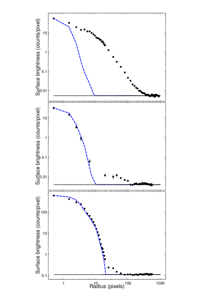
Figure 1: Three cases of AGN contamination. Top panel: the central AGN is strong but the cluster’s flux dominates; source is kept in the sample. Middle panel: AGN dominates over the clusters’ flux; the source is excluded from our sample. Bottom panel: The AGN is dominant and there is some evidence for the presence of extended emission; source is excluded from the sample. Black filled symbols represent the data while the modelled PSF is represented by the blue dashed line. The horizontal dotted line marks the background level.

3.1.4 Cooling Time

The mechanism by which gas in clusters of galaxies cools is radiation of its thermal energy through X-ray emission. One simple parameter which can characterize the thermal state of the gas is the cooling time, which is defined as the characteristic timescale on which the gas radiates away its thermal energy. The cooling time at a radius $r$ is

$$t_{cool}(r)=\dfrac{3}{2}\,\dfrac{\mu_{e}\,n_{e}\,V\,kT}{\mu\,L_{x}}\leavevmode\nobreak\ ,$$ (4)

where $kT$ and $n_{\mathrm{e}}$ are the gas temperature and electron number density in a spherical shell of volume $V$ at radius $r$, and $L_{\mathrm{x}}$ is the luminosity radiated by the shell. The mean mass per electron ($\mu_{\mathrm{e}}$) and mean mass per particle ($\mu$) have values of 1.15 and 0.597, respectively, corresponding to a fully ionized thermal plasma with metallicity 0.3 Z_⊙ (Sutherland & Dopita, 1993).

The gas density at radius $r$ is derived from the normalization of the thermal plasma fit to the source spectrum and derived counts emissivity using the following equation:

$$n_{e}(r)=\sqrt{\dfrac{(n_{e}/n_{H})\,N_{\rm spec}\,4\pi[D_{a}(1+z)]^{2}}{V\,10^{-14}}\dfrac{\epsilon(r)}{C}}\leavevmode\nobreak\ ,$$ (5)

where D_a is the angular diameter distance , $\epsilon(r)$ is the counts emissivity integrated over the volume of the shell (i.e. the total count/s from the shell) and C is the total number of counts from the source within $\mathrm{R_{500}}$. $N_{\rm spec}$ is the normalization of the thermal plasma model fitted to the spectrum extracted within $\mathrm{R_{500}}$, with all point sources excluded, which for the APEC model is related to the emission measure by

$N_{\rm spec}=\dfrac{10^{-14}}{4\pi[D_{a}(1+z)]^{2}}\int n_{e}n_{H}dV$.

The analytical expression for the counts emissivity profile

$$\epsilon(r)=\epsilon_{0}(1+(r/r_{c})^{2})^{-\eta}\leavevmode\nobreak\ ,$$ (6)

can be obtained from the surface brightness profile of the form given in Equation 3 by geometrical deprojection, assuming a spherically symmetric distribution. Since surface brightness represents the projection on the sky of emissivity, the surface brightness profile can be written as a integral along the line of sight of emissivity:

$$S(b)=2\int_{0}^{\infty}\epsilon(r)dl\leavevmode\nobreak\ ,$$ (7)

where $r^{2}=b^{2}+l^{2}$ and $l$ is the direction along the line of sight. Solving the integral, we can obtain the slope and the normalization of the emissivity profile as a function of the beta-model parameters. Hence $\eta=3\beta$ and $\epsilon_{0}=S_{0}/(2r_{c}\int_{0}^{\pi/2}\cos\alpha^{2(\eta-1)}d\alpha)$ .

The temperature of the gas is required to derive gas density from the emissivity, and hence to calculate entropy and cooling time. We use the global temperature, as our data quality does not allow us to construct temperature profiles. For CC systems, the temperature drops in the core, by a factor of up to 2 or 3 from its peak value (or a smaller factor compared to the mean global temperature). As a result, we will somewhat overestimate the central cooling time in CC systems, by a factor of approximately $\sqrt{2}$.

Clearly, the cooling time rises progressively with radius, as the density drops, so we need to pick a scale radius at which to extract the cooling time which will characterise the cluster core. We would like this radius to be as small as possible, subject to it being resolved in our observations. However, we do want the derived gas properties to represent the group/cluster core. Sun et al. (2007) has pointed out that some galaxy groups contain dense gas within the central galaxy, which he refers to as a ‘compact corona’. These small gas halos are distinct from classic cool cores and are more closely associated with the central galaxy itself. These compact coronae have sizes typically between 1-4 kpc (Vikhlinin et al., 2001; Sun et al., 2007), though they can be as large as 10 kpc. On the basis of these considerations, we pick our scale radius for calculation of the cooling time to be $0.01R_{500}$, which is deep inside the CC region even for low mass systems but generally outside the inner 4 kpc. Our surface brightness profiles have a radial resolution of $0.49\arcsec$, which is similar to the FWHM of the Chandra on-axis PSF. This corresponds to a physical scale of 4 kpc at z=1, and is smaller than $0.01R_{500}$ for all our systems apart from CDGS62 at z=1.27, for which 0.01$\mathrm{R_{500}}$ lies just inside the innermost bin. Although our cooling time is derived from the analytical emissivity profile fitted (allowing for PSF blurring) to the radial surface brightness profile, the value for CDGS62 should be regarded as slightly less robust than the others, since it involves a small extrapolation inwards from the innermost data bin.

3.1.5 Entropy

Another parameter which can be used to characterize the thermal state of the gas is its entropy, which we define here as $K=\dfrac{kT}{n_{e}^{2/3}}$. This definition is widely adopted in X-ray studies of clusters, and the standard thermodynamic definition of entropy can be obtained from it by applying a logarithm and adding a constant (Voit, 2005). To characterise the cluster core properties, we evaluate the entropy at a scale radius of $0.01R_{500}$.

3.1.6 Error calculation

Uncertainties in the values of $t_{\rm cool}$ and $K$ are estimated using Monte Carlo simulations. The density profile parameters and the temperature are perturbed in a Gaussian fashion based on their derived fitting errors. For each newly created set of parameters, a value for $t_{\rm cool}$ and $K$ at 0.01$\mathrm{R_{500}}$ is calculated. 1000 such random realisations are generated and the required errors are derived from the distribution of $t_{\rm cool}$ and $K$ which result. For the poorest quality datasets, the derived errors can be very large, as can be seen in Table 2.

3.2 Quantifying cool core status

In order to study the evolution of cooling in cluster cores, we need to choose an indicator of cool core strength. Ideally, this indicator should be able to distinguish CC and NCC systems in a way which is minimally affected by variations in redshift, temperature and data quality. As discussed earlier, several CC estimators have been used in the literature: some are based on the central temperature drop (Maughan et al., 2012), some quantify the central surface brightness excess (Maughan et al., 2012; Alshino et al., 2010; Santos et al., 2008), whilst others are based on physical characteristics like central cooling time or entropy (Peres et al., 1998; Bauer et al., 2005; Mittal et al., 2009).

Parameters that define the CC strength based on the amplitude of the central temperature drop observed in the temperature profile of the system are not accessible to us here because of the high quality data required to construct temperature profiles. As many of our systems lie not far above our 100 count lower limit, even calculating the ratio of central to outer temperature is not feasible. Central cooling leads to increased gas density, resulting in a sharp central cusp in surface brightness. This has been used to define a number of different CC diagnostics. These approaches have the advantage that they require only imaging data and can therefore be applied over a wide range in data quality. When defining these parameters, generally a size for the CC is assumed in order to separate the emission coming from the core from the larger scale emission.

Table 2: X-ray derived properties. Columns represent: 1) Source ID, which is the same as in Table LABEL:table:table1; 2) Number of soft source counts (0.5-2.0 keV); 3) $\mathrm{R_{500}}$estimated iteratively as explained in 3.1.1; 4) Gas temperature estimated from a thermal plasma model fit to a spectrum extracted within $\mathrm{R_{500}}$; 5) Cooling time; 6) Cooling time normalized by the age of the cluster which is the age of the Universe at the cluster’s redshift; 7) Entropy; 8)-10) Three cuspiness cool core indicators (see LABEL:subsection:cuspiness). All errors are $1\sigma$ errors. Errors for cooling time and entropy are calculated using Monte Carlo simulations (see 3.1.6), while errors in cuspiness cool core indicators are estimated based on error propagation. Unconstrained errors are marked with asterisks.

ID	Counts	$R_{500}$	kT	$t_{cool}$	$t_{cool}/t_{Uni}$	K	Csb	Fratio	Fc
		(Mpc)	(keV)	(Gyr)		(keV cm2)
CDGS1	2522	0.470	$0.98^{+0.18}_{-0.06}$	$1.12\pm 0.57$	$0.09\pm 0.04$	$22.95\pm 7.31$	$0.393\pm 0.606$	$0.402\pm 0.374$	$3.87\pm 0.26$
CDGS2	1008	0.519	$1.30^{+0.21}_{-0.06}$	$3.27\pm 6.12$	$0.27\pm 0.50$	$46.94\pm 42.62$	$0.139\pm 0.143$	$0.278\pm 0.208$	$1.62\pm 0.20$
CDGS3	1982	0.557	$2.08^{+1.83}_{-0.52}$	$16.81\pm 22.72$	$1.36\pm 1.85$	$156.47\pm 184.10$	$0.055\pm 0.008$	$0.173\pm 0.017$	$0.52\pm 0.08$
CDGS4	357	0.562	$1.54^{+0.46}_{-0.30}$	$1.57\pm 1.08$	$0.13\pm 0.09$	$29.48\pm 13.96$	$0.100\pm 0.024$	$0.152\pm 0.032$	$2.27\pm 0.64$
CDGS5	1047	0.492	$1.25^{+0.11}_{-0.14}$	$1.96\pm 0.91$	$0.17\pm 0.08$	$32.95\pm 9.24$	$0.153\pm 0.079$	$0.140\pm 0.105$	$1.79\pm 0.41$
CDGS6	2132	0.864	$3.42^{+0.80}_{-0.45}$	$22.19\pm 14.99$	$1.95\pm 1.32$	$244.52\pm 123.01$	$0.057\pm 0.008$	$0.195\pm 0.017$	$1.20\pm 0.19$
CDGS7	173	0.437	$1.01^{+0.19}_{-0.11}$	$4.26\pm 6.54$	$0.38\pm 0.58$	$55.70\pm 45.33$	$0.173\pm 0.055$	$0.360\pm 0.114$	$1.44\pm 0.50$
CDGS8	2413	0.708	$2.54^{+0.50}_{-0.49}$	$8.27\pm 1.99$	$0.74\pm 0.18$	$107.51\pm 28.49$	$0.048\pm 0.005$	$0.225\pm 0.013$	$0.61\pm 0.06$
CDGS9	910	0.778	$2.93^{+1.19}_{-0.62}$	$1.47\pm 1.25$	$0.13\pm 0.11$	$36.71\pm 24.66$	$0.157\pm 0.020$	$0.302\pm 0.031$	$1.88\pm 0.25$
CDGS10	17428	0.833	$3.42^{+0.20}_{-0.22}$	$1.67\pm 1.26$	$0.15\pm 0.11$	$43.69\pm 18.27$	$0.200\pm 0.004$	$0.509\pm 0.009$	$1.49\pm 0.04$
CDGS11	324	0.630	$1.83^{+1.00}_{-0.36}$	$3.80\pm 16.67$	$0.34\pm 1.51$	$56.18\pm 95.19$	$0.215\pm 0.297$	$0.343\pm 0.107$	$0.90\pm 0.21$
CDGS12	1528	0.660	$2.11^{+0.45}_{-0.27}$	$1.27\pm 0.62$	$0.12\pm 0.06$	$28.07\pm 9.81$	$0.137\pm 0.015$	$0.207\pm 0.018$	$2.39\pm 0.32$
CDGS13	1254	0.819	$3.37^{+0.95}_{-0.57}$	$9.96\pm 4.13$	$0.91\pm 0.38$	$142.31\pm 64.28$	$0.043\pm 0.008$	$0.167\pm 0.014$	$0.86\pm 0.10$
CDGS14	440	0.727	$2.77^{+2.64}_{-0.86}$	$1.27\pm 2.21$	$0.12\pm 0.21$	$32.36\pm 46.18$	$0.186\pm 0.028$	$0.357\pm 0.054$	$1.85\pm 0.27$
CDGS15	499	0.557	$1.76^{+0.55}_{-0.20}$	$0.71\pm 0.32$	$0.07\pm 0.03$	$17.79\pm 6.89$	$0.173\pm 0.029$	$0.250\pm 0.034$	$2.23\pm 0.42$
CDGS16	368	0.720	$2.99^{+1.22}_{-0.86}$	$10.07\pm 12.81$	$1.01\pm 1.29$	$133.72\pm 118.12$	$0.088\pm 0.021$	$0.295\pm 0.062$	$1.09\pm 0.36$
CDGS17	48672	1.107	$6.57^{+0.35}_{-0.22}$	$0.54\pm 0.06$	$0.05\pm 0.01$	$30.08\pm 2.79$	$0.216\pm 0.003$	$0.635\pm 0.005$	$2.17\pm 0.03$
CDGS18	733	0.662	$2.53^{+0.42}_{-0.29}$	$5.25\pm 3.00$	$0.53\pm 0.30$	$79.10\pm 31.32$	$0.085\pm 0.013$	$0.263\pm 0.027$	$0.86\pm 0.16$
CDGS19	516	0.735	$3.10^{+1.30}_{-0.73}$	$14.42\pm 9.86$	$1.47\pm 1.01$	$173.22\pm 101.88$	$0.055\pm 0.014$	$0.208\pm 0.034$	$0.77\pm 0.23$
CDGS20	1345	0.803	$3.52^{+0.76}_{-0.57}$	$6.23\pm 4.24$	$0.65\pm 0.44$	$106.58\pm 53.60$	$0.085\pm 0.010$	$0.234\pm 0.017$	$1.29\pm 0.19$
CDGS21	22738	1.221	$8.38^{+0.87}_{-0.41}$	$0.66\pm 0.05$	$0.07\pm 0.01$	$39.75\pm 4.10$	$0.224\pm 0.004$	$0.566\pm 0.006$	$1.94\pm 0.04$
CDGS22	639	0.668	$2.73^{+0.68}_{-0.51}$	$11.38\pm 5.50$	$1.20\pm 0.58$	$137.77\pm 54.19$	$0.050\pm 0.011$	$0.149\pm 0.021$	$0.86\pm 0.25$
CDGS23	203	0.558	$1.92^{+1.41}_{-0.32}$	$7.71\pm 9.43$	$0.83\pm 1.01$	$90.18\pm 88.01$	$0.084\pm 0.027$	$0.325\pm 0.073$	$0.96\pm 0.38$
CDGS24	675	0.553	$1.94^{+0.28}_{-0.22}$	$5.26\pm 3.66$	$0.57\pm 0.40$	$70.11\pm 33.75$	$0.081\pm 0.014$	$0.190\pm 0.023$	$1.25\pm 0.32$
CDGS25	14141	0.956	$5.59^{+0.25}_{-0.21}$	$0.39\pm 0.03$	$0.042\pm 0.003$	$22.06\pm 1.38$	$0.364\pm 0.006$	$0.715\pm 0.010$	$1.57\pm 0.03$
CDGS26	14546	0.956	$5.59^{+0.48}_{-0.36}$	$0.49\pm 0.03$	$0.053\pm 0.003$	$25.68\pm 2.22$	$0.272\pm 0.005$	$0.565\pm 0.008$	$1.94\pm 0.05$
CDGS27	10852	0.865	$4.59^{+0.43}_{-0.42}$	$0.76\pm 0.27$	$0.08\pm 0.03$	$30.68\pm 7.47$	$0.163\pm 0.005$	$0.324\pm 0.007$	$2.04\pm 0.09$
CDGS28	9837	0.897	$4.89^{+0.48}_{-0.25}$	$0.34\pm 0.03$	$0.038\pm 0.003$	$18.59\pm 1.91$	$0.330\pm 0.007$	$0.654\pm 0.011$	$1.91\pm 0.06$
CDGS29	17937	1.090	$7.10^{+0.58}_{-0.53}$	$0.93\pm 0.08$	$0.10\pm 0.01$	$45.50\pm 4.23$	$0.242\pm 0.005$	$0.554\pm 0.007$	$2.10\pm 0.05$
CDGS30	654	0.660	$2.66^{+0.45}_{-0.35}$	$2.84\pm 1.65$	$0.32\pm 0.19$	$54.02\pm 22.41$	$0.109\pm 0.016$	$0.311\pm 0.030$	$1.21\pm 0.26$
CDGS31	11194	1.013	$6.44^{+0.39}_{-0.55}$	$1.59\pm 0.17$	$0.18\pm 0.02$	$61.31\pm 6.64$	$0.170\pm 0.005$	$0.619\pm 0.010$	$1.27\pm 0.04$
CDGS32	205	0.476	$1.57^{+0.24}_{-0.20}$	$2.48\pm 2.80$	$0.28\pm 0.32$	$40.00\pm 25.63$	$0.095\pm 0.027$	$0.259\pm 0.054$	$1.00\pm 0.26$
CDGS33	428	0.664	$3.01^{+0.93}_{-0.94}$	$12.20\pm 7.38$	$1.40\pm 0.84$	$152.60\pm 74.42$	$0.078\pm 0.019$	$0.208\pm 0.034$	$0.99\pm 0.32$
CDGS34	20101	1.392	$12.36^{+0.73}_{-0.63}$	$7.60\pm 0.40$	$0.90\pm 0.05$	$248.07\pm 15.62$	$0.032\pm 0.002$	$0.229\pm 0.004$	$0.70\pm 0.03$
CDGS35	1745	0.763	$4.18^{+0.39}_{-0.37}$	$12.29\pm 1.06$	$1.48\pm 0.13$	$185.34\pm 19.19$	$0.029\pm 0.005$	$0.128\pm 0.010$	$0.51\pm 0.11$
CDGS36	1142	0.625	$2.87^{+0.41}_{-0.58}$	$5.05\pm 1.65$	$0.61\pm 0.20$	$82.47\pm 23.62$	$0.097\pm 0.011$	$0.282\pm 0.021$	$1.01\pm 0.17$
CDGS37	11370	1.077	$7.96^{+0.35}_{-0.36}$	$9.76\pm 0.32$	$1.20\pm 0.04$	$233.19\pm 10.84$	$0.032\pm 0.002$	$0.248\pm 0.006$	$0.59\pm 0.04$
CDGS38	1850	0.821	$4.83^{+0.85}_{-0.95}$	$1.18\pm 0.55$	$0.14\pm 0.07$	$42.45\pm 14.67$	$0.104\pm 0.009$	$0.339\pm 0.018$	$1.17\pm 0.14$
CDGS39	193	0.751	$3.58^{+9.00}_{-1.53}$	$0.63\pm 1.18$	$0.08\pm 0.15$	$23.35\pm 54.95$	$0.328\pm 0.059$	$0.713\pm 0.167$	$1.17\pm 0.19$
CDGS40	127	0.685	$3.58^{+21.56}_{-1.75}$	$4.31\pm 15.85$	$0.55\pm 2.04$	$84.13\pm 429.50$	$0.103\pm 0.037$	$0.345\pm 0.084$	$1.05\pm 0.47$
CDGS41	2725	0.507	$2.16^{+1.11}_{-0.35}$	$16.00\pm 18.03$	$2.12\pm 2.38$	$153.01\pm 134.27$	$0.046\pm 0.009$	$0.104\pm 0.072$	$0.84\pm 0.19$
CDGS42	330	0.450	$1.67^{+1.65}_{-0.93}$	$6.57\pm 49.42$	$0.87\pm 6.55$	$77.21\pm 164.94$	$0.119\pm 0.035$	$0.228\pm 0.059$	$1.60\pm 0.59$
CDGS43	1478	0.791	$4.92^{+0.48}_{-0.40}$	$3.90\pm 0.78$	$0.52\pm 0.10$	$95.14\pm 15.49$	$0.074\pm 0.008$	$0.397\pm 0.022$	$0.75\pm 0.10$
CDGS44	2526	0.972	$7.37^{+1.78}_{-1.46}$	$11.80\pm 4.08$	$1.58\pm 0.55$	$253.74\pm 83.36$	$0.035\pm 0.005$	$0.194\pm 0.010$	$0.59\pm 0.08$
CDGS45	1334	0.777	$4.98^{+0.86}_{-0.47}$	$5.76\pm 2.14$	$0.79\pm 0.29$	$124.31\pm 36.34$	$0.063\pm 0.008$	$0.292\pm 0.020$	$0.80\pm 0.13$
CDGS46	1033	0.695	$4.13^{+0.86}_{-0.74}$	$4.06\pm 1.33$	$0.56\pm 0.18$	$87.89\pm 25.12$	$0.099\pm 0.012$	$0.341\pm 0.025$	$0.80\pm 0.14$
CDGS47	1262	0.757	$5.00^{+1.56}_{-1.68}$	$16.36\pm 4.52$	$2.25\pm 0.62$	$249.86\pm 93.94$	$0.028\pm 0.006$	$0.122\pm 0.013$	$0.53\pm 0.13$
CDGS48	1496	0.610	$3.31^{+1.19}_{-0.75}$	$16.40\pm 12.87$	$2.25\pm 1.77$	$195.69\pm 121.22$	$0.080\pm 0.089$	$0.110\pm 0.034$	$0.95\pm 0.16$
CDGS49	542	0.550	$2.53^{+0.88}_{-0.60}$	$1.71\pm 2.29$	$0.24\pm 0.32$	$37.34\pm 32.01$	$0.160\pm 0.026$	$0.292\pm 0.051$	$1.53\pm 0.29$
CDGS50	1531	1.063	$9.31^{+7.81}_{-4.54}$	$8.68\pm 4.91$	$1.22\pm 0.69$	$237.14\pm 171.73$	$0.057\pm 0.007$	$0.512\pm 0.033$	$0.73\pm 0.08$
CDGS51	3730	0.882	$6.68^{+1.00}_{-0.75}$	$3.02\pm 0.48$	$0.43\pm 0.07$	$96.74\pm 16.53$	$0.097\pm 0.006$	$0.432\pm 0.014$	$0.97\pm 0.07$
CDGS52	321	0.627	$3.34^{+1.69}_{-0.80}$	$3.18\pm 3.09$	$0.46\pm 0.45$	$65.97\pm 52.96$	$0.126\pm 0.027$	$0.224\pm 0.038$	$1.49\pm 0.49$
CDGS53	340	0.566	$2.85^{+1.14}_{-0.75}$	$5.66\pm 45.89$	$0.84\pm 6.80$	$88.40\pm 163.53$	$0.120\pm 0.027$	$0.346\pm 0.083$	$0.78\pm 0.22$
CDGS54	594	0.666	$4.36^{+2.27}_{-2.15}$	$3.87\pm 4.79$	$0.60\pm 0.75$	$87.90\pm 84.47$	$0.093\pm 0.015$	$0.252\pm 0.028$	$1.07\pm 0.20$
CDGS55	620	0.679	$5.44^{+8.15}_{-2.48}$	$1.70\pm 10.42$	$0.28\pm 1.69$	$58.40\pm 216.32$	$0.242\pm 0.063$	$1.061\pm 0.367$	$1.03\pm 0.13$
CDGS56	1781	0.980	$10.43^{+5.87}_{-3.32}$	$3.41\pm 1.78$	$0.57\pm 0.30$	$136.92\pm 80.37$	$0.105\pm 0.009$	$0.406\pm 0.021$	$1.21\pm 0.12$
CDGS57	1200	0.722	$5.98^{+2.13}_{-1.03}$	$0.58\pm 0.86$	$0.10\pm 0.15$	$30.05\pm 27.71$	$0.139\pm 0.013$	$0.352\pm 0.022$	$1.39\pm 0.18$
CDGS58	385	0.577	$4.75^{+1.82}_{-1.69}$	$7.43\pm 8.63$	$1.33\pm 1.54$	$143.06\pm 102.50$	$0.098\pm 0.019$	$0.300\pm 0.042$	$0.83\pm 0.23$
CDGS59	313	0.444	$2.57^{+0.37}_{-0.33}$	$0.40\pm 8.35$	$0.07\pm 1.50$	$14.18\pm 57.47$	$0.073\pm 0.018$	$0.156\pm 0.029$	$1.88\pm 0.61$
CDGS60	757	0.664	$6.07^{+2.87}_{-1.27}$	$4.38\pm 2.59$	$0.86\pm 0.51$	$116.94\pm 67.07$	$0.090\pm 0.014$	$0.268\pm 0.026$	$0.98\pm 0.21$
CDGS61	351	0.621	$6.50^{+4.10}_{-3.05}$	$7.61\pm 23.68$	$1.51\pm 4.70$	$176.47\pm 251.38$	$0.109\pm 0.021$	$0.288\pm 0.045$	$1.00\pm 0.28$
CDGS62	124	0.331	$1.81^{+0.68}_{-0.59}$	$3.64\pm***$	$0.73\pm***$	$53.11\pm***$	$0.118\pm 0.044$	$0.147\pm 0.049$	$0.74\pm 0.55$

Table 2: continued

It is not a priori clear what scale should be chosen to separate core from cluster emission. Maughan et al. (2012) use a fraction of $\mathrm{R_{500}}$, whilst Santos et al. (2008) argue that cluster cores cannot be expected to evolve in a self-similar fashion and so use a fixed metric radius of 40 kpc.

Given the wide mass and redshift ranges spanned by our sample, the choice of core radius has a significant impact, and is therefore a disadvantage for these methods. We therefore prefer to base the bulk of our analysis on more physically motivated CC indicators. However, in Section LABEL:subsection:cuspiness, we calculate some these cuspiness indicators for our sample, and compare the results with those from our preferred methods.

Central cooling time and entropy are gas properties which are well-established to differ between CC and NCC clusters. Both are determined primarily by gas density and temperature, though cooling time is also affected by metallicity, which we take to be 0.3 solar. As a result, the two properties are closely related. Cooling time ($t_{\rm cool}$) is more directly related to the cooling status of the system, so we use this for preference. As discussed in Section 3.1.4 above, our ‘central’ cooling time is actually calculated at a radius 0.01$\mathrm{R_{500}}$.

It will be helpful for some of our analysis to adopt a threshold value for $t_{\rm cool}$ to mark the transition between CC and NCC systems. Previous studies in which central cooling time is used as a CC diagnostic have used a variety of cooling time thresholds, ranging from 0.8 Gyr up to the age of the Universe (Peres et al., 1998; Bauer et al., 2005; Mittal et al., 2009). To help motivate our own choice, we note that some studies of the distribution of central entropy in groups and clusters have shown the existence of bimodality (Cavagnolo et al., 2009; Sanderson et al., 2009; Mahdavi et al., 2013). Moreover, Cavagnolo et al. (2008) show that systems with a central entropy lower than 30 keV cm² show evidence for gas cooling at the cluster centre, in the form of optical emission lines.

Although both the Cavagnolo and Mahdavi studies show the existence of bimodality in the entropy distribution, the break between the two peaks occurs at 30-50 keV cm² for Cavagnolo et al. (2009) but 70 keV cm² for Mahdavi et al. (2013). However, the difference between these two values can be explained by the difference in the radius at which the entropy has been calculated. This is effectively the centre in the former case, but is 20 kpc for the latter.

Since our measurement is closer to the first of these, we adopt a cooling time threshold corresponding to a central entropy of 40 keV cm², which lies within the 30-50 keV cm² interval from Cavagnolo et al. (2009). The tight correlation between our cooling time and entropy values is shown in Figure LABEL:figTK. Since entropy scales as $T/n_{e}^{2/3}$, whilst cooling time scales (in the bremsstrahlung regime) as $T^{1/2}/n_{e}\propto K^{3/2}/T$, we see that there is some offset in the Figure between groups and clusters, such that the gas in clusters has a rather shorter cooling time at given entropy. Averaging over our sample, we adopt 1.5 Gyr as a sensible cooling time threshold.

An important issue, highlighted in the recent study by McDonald et al. (2013), is the distinction between the rate of current cooling and the amount of gas which has been able to cool. $t_{\rm cool}$ is a measure of the former, but for a cluster at high redshift less time has been available for cooling to take effect. Since both current cooling and the accumulated effects of cooling are of interest to us, we construct a further cool core indicator, $t_{\rm cool}/t_{\rm Uni}$, in which cooling time is divided by the age of the Universe ($t_{\rm Uni}$) in our adopted cosmology, at the redshift of the cluster. This represents the fraction of gas which could have cooled in the lifetime of the cluster, in the absence of AGN feedback. In practice, the impact of AGN feedback is believed to suppress gas cooling by an order of magnitude (McNamara & Nulsen, 2012), but cannot prevent it altogether. In these circumstances, the integrated fraction of a cluster’s gas which could have cooled over its history should still scale roughly with $t_{\rm cool}/t_{\rm Uni}$, though the impact of cyclic AGN activity on the cooling time in the core will introduce considerable scatter.

We calculate the threshold value for this parameter, separating CC from NCC systems, by dividing the threshold used for $t_{\rm cool}$ (1.5 Gyr) by the age of the Universe at the median redshift of systems from our sample (8.7 Gyr). This gives a threshold value for $t_{\rm cool}/t_{\rm Uni}$ of 0.17, which will be used below.

4 Results

4.1 Cool core evolution

The evolution of CC strength, as quantified by $t_{\rm cool}$ and $t_{\rm cool}/t_{\rm Uni}$, as well as entropy, all evaluated at radius 0.01$\mathrm{R_{500}}$, is shown in Figure LABEL:fig2. For each parameter, we plot the results obtained when using the entire sample (left panel), a subsample which contains only clusters ($T\geq 3$ keV, middle panel) and one which contains only groups (right panel). This temperature cut allows us to compare the behaviour of evolutionary trends in the two mass regimes.

In each panel, black points represent the data, whilst the contoured colour scale traces the smoothed density of points. The black dotted line shows the threshold adopted for separating CC from NCC systems (0.17 for $t_{\rm cool}/t_{\rm Uni}$, 1.5 Gyr for cooling time and 40 keV cm² for entropy). In each case, CC systems lie below the line.

A broadly similar pattern is seen in all three rows. Some bimodality is apparent in the distribution for all three parameters. This bimodality is more pronounced in the cluster sub-population, whilst in groups the pattern is quite similar, but the CC and NCC peaks move closer together and merge into a single elongated distribution.

Examining density plots such as Figure LABEL:fig2 is not a reliable way of establishing evolutionary trends. For example, the shape of the density contours can be substantially modified by transformations of the axes (plotting the cool core indicators in unlogged form, for example). We have therefore tested for correlations of our CC indicators with redshift by calculating the Spearman rank correlation coefficient. The results are shown in the first three rows of Table LABEL:Spearman. Values for our X-ray selected sample occupy the left hand side of the Table. Corresponding values for our ‘extended sample’ will be discussed later, in Section LABEL:subsec:extended_results.

	X-ray selected sample						Extended sample
Parameter	All sample		Clusters		Groups		All sample		Clusters		Groups
	Coeff	P-val	Coeff	P-val	Coeff	P-val	Coeff	P-val	Coeff	P-val	Coeff	P-val
$\mathbf{t}_{\bf\rm cool}/\mathbf{t}_{\bf\rm Uni}$	0.26	0.04	0.27	0.12	0.28	0.17	0.29	0.006	0.29	0.03	0.35	0.06
$\mathbf{t}_{\bf\rm cool}$	0.07	0.58	0.12	0.49	0.14	0.49	0.11	0.35	0.14	0.30	0.19	0.32
K	0.26	0.04	0.22	0.20	0.17	0.41	0.29	0.006	0.24	0.07	0.22	0.25
$\mathbf{c}_{\bf\rm SB}$	-0.17	0.19	-0.09	0.59	-0.31	0.12	-0.24	0.03	-0.18	0.18	-0.38	0.04
$\mathbf{F}_{\bf\rm core}$	0.04	0.74	-0.07	0.70	-0.15	0.45	-0.06	0.57	-0.16	0.24	-0.26	0.17
$\mathbf{f}_{\bf\rm c}$	-0.35	0.005	-0.35	0.03	-0.33	0.10	-0.34	0.001	-0.29	0.03	-0.36	0.05

The Table gives the values of the correlation coefficient for a trend in each CC indicator with redshift. Being a rank correlation coefficient, this is independent of any monotonic transformation of either axis. For each coefficient, the chance probability (2-tailed) of obtaining a value deviating from zero by this value or more is also quoted.

As can be seen, a significant trend ($p=0.04$) is apparent in $t_{\rm cool}/t_{\rm Uni}$ (and to a lesser extent in entropy) for both the full (cluster $+$ group) sample, and for clusters alone. The group subsample shows a correlation coefficient of similar size, but this is less significant, given the smaller number of systems involved. However, the $t_{\rm cool}$ indicator shows no significant trend with redshift.

As a further test, we examine the distribution of our two main CC indicators across the sample at low and high redshift, and apply a Kolmogorov-Smirnov (K-S) test to see whether they differ. We choose a redshift cut at 0.5 to separate the low and high redshift samples for this test, motivated by previous results in the literature which report a change in the properties of CCs at redshifts greater than 0.5 (Vikhlinin et al., 2007). However we have tested various redshift thresholds and find similar results for any cut between 0.5 and 0.65. For $t_{\rm cool}/t_{\rm Uni}$ we find a highly significant difference ($p=0.009$) between the distributions at high and low redshift. As shown in Figure LABEL:fig3, our low redshift systems are more strongly concentrated towards low values of $t_{\rm cool}/t_{\rm Uni}$, confirming the redshift trend indicated by the Spearman rank analysis. Performing a similar analysis for $t_{\rm cool}$ we find a much weaker difference between the high and low redshift distributions, though it can still be significant, depending on the value of the redshift cut. We will return to this with our larger ‘extended sample’ in Section LABEL:subsec:extended_results below.

Returning to the interpretation of our two main CC indicators as representing current cooling ($t_{\rm cool}$) and accumulated cooling ($t_{\rm cool}/t_{\rm Uni}$) in the core, our conclusion at this stage seems to be that the latter is evolving, whilst the former is not. However, before we can draw such a conclusion, we need to examine the possibility that the trends we see could be driven primarily by a changing composition in cluster richness with redshift, rather than evolution in properties for clusters at a given richness. Despite the rather similar behaviour in clusters and groups seen in Figure LABEL:figTK, it is well known that groups have gas properties which differ systematically from richer clusters – with flatter surface brightness profiles (Ponman et al., 1999) and more compact central cooling regions (Rasmussen & Ponman, 2007).

In Figure LABEL:figTz we examine the distribution in system temperature with redshift within our sample. As expected, the galaxy groups ($T<3$ keV), which are less luminous X-ray sources, are concentrated towards lower redshifts. However, interestingly this effect is largely confined to $z<0.35$, and above this redshift, the mean temperature of our sample is essentially constant, at around 4.5 keV. We have already seen that our conclusions about the trend in $t_{\rm cool}/t_{\rm Uni}$ and the lack of evolution in $t_{\rm cool}$ apply even if we exclude groups from our analysis. If we instead retain the full temperature range, but exclude all systems with $z<0.35$, a positive correlation (coefficient=0.21) remains, but its significance is reduced, due to the smaller sample and reduced redshift baseline. We conclude that our results are not being driven by redshift-dependent temperature biases in the sample.

4.2 Cuspiness cool core indicators

As we discussed earlier, most previous studies of cool core evolution have been based on an analysis of central surface brightness excess. We now apply some of these estimators to our own sample, for comparison with our above findings based on cooling time, and with results of earlier studies. We use three CC estimators defined in the literature: surface brightness concentration($c_{\rm SB}$; Santos et al. (2008)), the core flux ratio ($F_{\rm core}$; Maughan et al. (2012)) and the central excess factor($f_{\rm c}$; Alshino et al. (2010)), for which we employ the same symbols as the original authors.

The $c_{\rm SB}$ parameter is defined as the ratio between the flux measured within circular apertures with radii of 40 kpc and 400 kpc, centred on the peak of the cluster X-ray emission. These radii were found by Santos et al. (2010) to optimize the separation between CC and NCC in a sample of simulated low redshift clusters. They motivated the use of a fixed physical radius rather than a fraction of the scale radius, $\mathrm{R_{500}}$, by the fact that cool cores are the result of non-gravitational processes and therefore their sizes do not scale self-similarly. In their study, Santos et al. (2010) used $c_{\rm SB}$ to divide the sample into strong (SCC), weak (WCC) and non cool core (NCC) classes, with $c_{\rm SB}$$>0.155$, $0.075\leq$$c_{\rm SB}$$\leq 0.155$, and $c_{\rm SB}$$<0.075$, respectively.

Similar to the $c_{\rm SB}$ parameter is the $F_{\rm core}$ parameter, which is defined also as a flux ratio, but with aperture radii defined as fractions of $R_{500}$ instead of fixed physical sizes. Following Maughan et al. (2012), $F_{\rm core}$ is taken to be the ratio of flux within $0.15R_{500}$ to that within $R_{500}$. We add that while the definition of this parameter is similar to the one used by Maughan et al. (2012), the way in which we calculate the fluxes is based only upon imaging data, whilst Maughan et al. (2012) calculate the unabsorbed flux from spectra extracted within each aperture. If the core flux is greater than half of the flux within $R_{500}$ (i.e. $F_{\rm core}$$>0.5$), the system is characterized as a CC.

While $c_{\rm SB}$ and $F_{\rm core}$ are simple parameters which do not require any modelling of the data, the $f_{\rm c}$ parameter of Alshino et al. (2010) quantifies the strength of a CC using the central excess in surface brightness profile above a fitted beta model with a fixed core radius of $0.105R_{500}$. This core radius was chosen by Alshino et al. (2010) to correspond to the observed size of cores seen in the group-scale emission of well-resolved low redshift groups of galaxies by Helsdon & Ponman (2000). A CC is deemed to be present if the ratio ($f_{\rm c}$) of the observed flux within $0.05R_{500}$ to the corresponding flux derived from the fitted beta model (with core radius of $0.105R_{500}$) is greater than unity.

All three of these CC indicators have been found by their proponents to show evolutionary trends, so we investigate their relationship with our $t_{\rm cool}$ indicator. Figure LABEL:figIndicators shows in each panel the correlation between $t_{\rm cool}$ and the three surface brightness based CC estimators. Different symbol styles and colours differentiate groups and clusters, and the presence of a central black point denotes systems characterized as CC according to the y-axis parameter. (For $c_{\rm SB}$ we use the SCC criterion.) We have marked on the x-axis the value $t_{\rm cool}$=1.5 which is our adopted CC threshold.

Note that, in contrast to our calculation of $t_{\rm cool}$ and $t_{\rm cool}/t_{\rm Uni}$, no correction for any central AGN has been applied when calculating the surface brightness cuspiness indicators. Hence clusters with a bright central AGN will be biased towards showing CC properties. As we discuss later in Section LABEL:subsection:detbias, the indications are that AGN contamination is not a major problem in our sample.

Firstly, ignoring the distinction between groups and clusters, it can be seen that the best correlation with $t_{\rm cool}$ is found for $c_{\rm SB}$. We have calculated the Spearman coefficient for all parameters and find the highest coefficient for $c_{\rm SB}$ (-0.82), closely followed by $f_{\rm c}$ (-0.77), while the lowest correlation is found for the $F_{\rm core}$ parameter (Spearman coefficient of -0.60).

The correlation between $c_{\rm SB}$ and $t_{\rm cool}$ is much stronger than that between $F_{\rm core}$ and $t_{\rm cool}$, although both parameters are defined as the flux ratio between the core and the bulk of the system, the only difference being in the sizes adopted for the inner and outer regions. Before drawing any conclusions about this discrepancy, we remind the reader that each CC indicator has been optimized to be applied to samples dominated by either clusters ($c_{\rm SB}$ and $F_{\rm core}$) or groups ($f_{\rm c}$), while our sample includes both types of system. Therefore we compare the performance of each parameter on the system class for which it has been designed.

Applying $c_{\rm SB}$ and $F_{\rm core}$ to just our cluster subsample, we see that both parameters give similar strong correlations: -0.85 ($F_{\rm core}$) and -0.89 ($c_{\rm SB}$). However, for the group subsample, there is a large discrepancy in the correlation coefficients: -0.64 for $c_{\rm SB}$ and -0.17 for $F_{\rm core}$. The poor correlation seen for $F_{\rm core}$ in the case of groups can be explained by the large size of the radius chosen to characterize the core region ($0.15R_{500}$). For clusters, this is approximately the size of the cool core, when it is present, whilst in groups cores are smaller, extending to a radius of typically only $0.1R_{500}$ (Rasmussen & Ponman, 2007).

Comparing the symbols marked by black circles in Figure LABEL:figIndicators with the position of the vertical dashed line, we can examine the fraction numbers of CC systems amongst groups and clusters identified by each method. The $c_{\rm SB}$ indicator shows excellent agreement with $t_{\rm cool}$ when applied to clusters, whilst for groups it identifies a similar total number of CC systems, but not necessarily the same ones. For $F_{\rm core}$, the clusters characterized as CC are again similar to those identified by $t_{\rm cool}$, but not a single group is classified as a CC. $f_{\rm c}$ identifies fewer CC clusters than $t_{\rm cool}$, but includes some groups with rather long cooling times as being CC systems.

In Figure LABEL:figIndEvol we plot the distribution of the surface brightness based CC estimators against redshift, in a similar fashion to Figure LABEL:fig2. Note that for these three estimators high values correspond to strong cool cores, in contrast to our three previous estimators. We have therefore flipped the y axis scales so that core dominance still increases downward on each plot. For the $c_{\rm SB}$ plot, the two horizontal lines correspond to the two thresholds used by Santos et al. (2008), dividing clusters into SCC (bottom), WCC (middle) and NCC (top) classes.

The distributions for all three indicators show similarities with our earlier cooling time and entropy based parameters. In particular, all show some signs of bimodality, at least for clusters. In the case of $c_{\rm SB}$, there is the wide variety in the CC strength at low redshifts, while for redshifts greater than 0.6 the NCC and SCC classes largely disappear, leaving only WCC systems. $F_{\rm core}$ shows a similar pattern of narrowing towards intermediate core strength at $z>0.7$, whilst $f_{\rm c}$ shows less symmetrical behaviour.

Results from Spearman rank tests for correlation with redshift are shown in the bottom three rows of Table LABEL:Spearman, and confirm the visual impression from Figure LABEL:figIndEvol. For the X-ray sample (left hand side of Table LABEL:Spearman) only $f_{\rm c}$ shows a significant evolutionary trend. This correlation (negative, due to the reversed sense of the indicator compared to the physically based indicators shown in the first three rows of the Table) is apparent for clusters and groups individually, as well as for the combined sample.

4.3 Systems with photometric redshift

The majority of the sample used in this study (presented in Table LABEL:table:table1 and Table LABEL:table:table2) consists of groups and clusters, detected as extended sources in X-ray images, whose nature is confirmed through spectroscopic redshifts of galaxy members. However, for 23$\%$ (14 out of 62) of the sample no spectroscopic redshift was available in the literature, and the redshift used in our analysis is photometric.

While the accuracy of cluster photometric redshifts is typically at a level of $\sim∼0.02-0.05$ out to redshift of 1 (Bahcall et al., 2003; Koester et al., 2007; Pelló et al., 2009; Takey et al., 2013), which is perfectly adequate for our purposes, occasional ‘catastrophic errors’ in photometric redshifts can be up to an order of magnitude higher (Mullis et al., 2003; Koester et al., 2007; Pelló et al., 2009). Moreover, in the absence of spectroscopic confirmation that associated galaxies are really clustered in redshift, the identification of a cluster must be regarded as provisional.

We have therefore examined the effects of excluding the systems with photometric redshifts from our analysis. This produces no significant difference in our results. The nature of the trends seen do not change, but some become rather stronger. The most noticeable differences are found for the evolutionary trends in the cluster subsample for $t_{\rm cool}/t_{\rm Uni}$  (Spearman’s rank coefficient of 0.40; p-val=0.02), $t_{\rm cool}$(coefficient=0.25; p-val=0.16) and K(coefficient=0.34; p-val=0.06), which can be compared with the values in Table LABEL:Spearman. In addition, the trends seen in $c_{\rm SB}$for the full sample (coefficient=-0.25; p-val=0.07) and the group subsample (coefficient=-0.44; p-val=0.06) become more significant.

5 Selection biases and AGN contamination

Before drawing conclusions about the evolution of CCs in groups and clusters of galaxies we must consider first whether any differences seen between the core properties of high and low redshift systems might simply result of the way in which our sample has been selected.

Our X-ray selected sample, constructed from extended sources detected in Chandra archival observations which meet the criteria mentioned in Section 2, contains two classes of systems: (i) groups and clusters which represent the target of the Chandra observation, and (ii) serendipitously detected sources. Figure LABEL:fig:PtSer shows the $t_{\rm cool}$ distribution plot for the full X-ray sample, marking targetted and serendipitous sources with open and filled symbols respectively. It can be seen that targetted sources account for the majority of the sample at $z>0.7$.

The inclusion of deliberately targetted sources in our sample might introduce bias in favour of systems with a particular morphology or special properties, since these systems may have been observed because of these characteristics. While this kind of bias, known as archival bias affects only the non-serendipitous sources, a bias to which both types of systems are subject is detection bias. This is due to the effect of source properties on the efficiency with which they can be detected in an X-ray image. We now examine both these sources of bias in turn.

5.1 Detection biases

When constructing an X-ray selected sample of clusters, the probability that a system with a given flux and size will be included in it depends on the source detection efficiency and the ability to characterize the detected system as extended when compared to the telescope’s point spread function.

As detection probability is a function of both the flux and spatial distribution of the X-ray emission, a different detection efficiency may be expected for sources with different intrinsic properties such as core size (Eckert et al., 2011), substructure, and the presence of intracluster point sources (Vikhlinin et al., 1998; Burenin et al., 2007). For a given source flux, the detection probability may be increased by concentrating more of the flux in the core, until the concentration becomes so great that the cluster is rejected as appearing point-like.

Such an effect could, for example, account for the narrowing in core strength seen with the $c_{\rm SB}$ indicator at high redshift, if our detection method preferentially excludes systems with very large and very small core radii.

One way to check this hypothesis is by answering the following question: supposing that strong CC and NCC systems are common at high redshift, would we be able to detect such clusters with a flux value corresponding to our threshold limit of 100 soft band counts?

To answer this question we applied our detection algorithm to simulated observations of a high redshift CC and NCC cluster respectively. Observations were generated using the Chandra simulation software (MARX), which requires as input information about the system’s spectral properties and its spatial distribution, in the form of a spectrum and values for beta model parameters, respectively. We base the properties on an observed high redshift cluster, but perturb its surface brightness distribution to generate an extreme CC and NCC system. Our template system is the cluster from our sample (Table LABEL:table:table1) detected in CLJ1415.1+3612 field (CDGS57). This is a $\sim 6$ keV system at redshift 1.03. This provides the template for our input spectrum to MARX. For the spatial properties, we use the beta and normalization derived from our fit to the surface brightness profile of the CLJ1415.1+3612 cluster, but we perturb the core radius – to $0.007R_{500}$ to represent a SCC and $0.3R_{500}$ for a NCC profile, where $R_{500}$ is the overdensity radius of our template system. These two values for core radius represent the median values for the size of core radii as a fraction of $R_{500}$ for the low redshift ($z<0.3$) CC ($t_{\rm cool}$$<1.5$ Gyr) and strongly NCC (for which we adopt $t_{\rm cool}$$>7$ Gyr) systems in our sample. Having chosen the spectral and spatial parameters, we varied the exposure time of our simulations to obtain 100 soft band counts, which represents our threshold limit for source selection.

So far, these simulated observations do not include any contribution from the background, which will degrade the source detection probability. To account for this, we added our simulated images to the observed image of our template cluster. Having the background level and spectral properties of a real detected system, we can now test if detection would still be possible in the case of CC and NCC cases. When we applied our detection and extension test procedure, we were able to reliably detect as extended sources both the CC system and the NCC one. This indicates that at our 100 count limit, the sample is not significantly affected by biases in detection efficiency due to the size of the core. Had we included much fainter sources in our sample, this would undoubtedly not have been the case.

Another potential source of detection bias is the presence of intracluster point sources, especially central AGN which have a double influence on the detection efficiency. In the first case, point sources embedded in the intracluster medium can cause a positive bias, increasing the detection efficiency due to the central flux excess they add to the surface brightness distribution. On the other hand, there can be a negative bias if a bright AGN at the centre of a cluster dominates the cluster emission and leads to a misclassification of the cluster as a point source. Burenin et al. (2007) showed that the detection efficiency of a cluster varies in the presence of a central AGN according to the luminosity ratio between the AGN and the intracluster medium. The detection efficiency is raised if an AGN with a luminosity much less than that of the cluster is present. However, if the luminosity of the AGN dominates the cluster emission, the detection efficiency drops dramatically.

Our procedure for identifying central AGN was described in Section 3.1.3, and 7 cases fell into our AGN ‘class 1’, in which we were able to remove the central point source and analyse the cluster containing it. These systems are flagged with asterisks in Figure LABEL:fig:PtSer. A strong connection between the presence of a central AGN and CC status is apparent – most systems with a central point source are CCs. (Stott et al., 2012) showed that radio loud BCGs are more likely to be found in more massive systems and at the centre of CCs. Also, based on the observed correlation between the strength of CC and the radio power of the central AGN (Mittal et al., 2009), we might expect that, at least for clusters, high redshift systems dominated by strong AGN will be SCCs. Is it possible that this has introduced a bias against their inclusion in our sample?

The literature is limited in the number of X-ray studies of high redshift clusters with dominant central AGN. Two which have been studied are PKS1229-021 (Russell et al., 2012) and 3C186 (Siemiginowska et al., 2010). Both lie at $z>1$ and have been reported to contain a strong CC. Since these two systems were observed with ACIS-S, they were not included in our sample, which concentrated on ACIS-I observations. We have analysed the Chandra data for these sources and checked into which of the previously mentioned AGN classes they would fall, had they been part of our sample. They would fall into our first AGN class – sources with clear signs of extension in which the central AGN does not dominate the total flux. We conclude from this that, at least for massive systems detected in observations with exposures of at least 70 ks like ours, we are not strongly biased against CCs. This may not be the case for less massive systems.

To further examine the impact of central AGN on our results, we show in Figure LABEL:figAGN the X-ray luminosity of the cluster and AGN emission in sources which appeared from our analysis to contain both point-like and extended components, and are confirmed from the literature to involve both an AGN and a cluster.

Points marked in red correspond to the AGN (asterisk symbols) and cluster (filled circles) contributions to the 7 systems in which we were able to remove the AGN component and still perform a useful analysis on the remaining cluster emission. The green points correspond to clusters which were excluded from our sample, since the remaining cluster component after removal of the central point source did not leave enough signal/noise for a reliable analysis.

Finally, we also mark (blue labelled symbols) the location of PKS1229-021 and 3C186. The luminosities here have been estimated by fitting a point source plus beta-model distribution to the X-ray surface brightness distribution. For the green points, where the cluster contribution is weak, the cluster luminosities should be regarded as rough estimates.

Most of the systems (red points) in which we have been able to successfully remove AGN contamination contain AGN which are less luminous than the cluster gas. The only exception to this is the lowest redshift system, which is a nearby galaxy group ($T\approx 1$ keV) with a correspondingly large X-ray extent. The clusters in which we were unable to perform a useful analysis after removing the central AGN (green points) have AGN which are brighter than the cluster, apart from the two systems at $z=0.8$-1.0. These two are both observed at large off-axis angles, where the instrument point spread function is broader, and the central AGN contaminates a region about $20\arcsec$ in diameter.

In general, our results suggest that the problem of AGN contamination is a modest one in our sample. At low redshift ($z<0.5$), we find that about 19% of our detected clusters contain central X-ray AGN, and in most of these the AGN contributes less than 10% of the cluster luminosity. With the exception of PKS1229-021 and 3C186, which were not part of our sample and were specially added to examine the case of powerful central AGN at high redshift, there is little sign in Figure LABEL:figAGN that the luminosity of central AGN is increasing at redshifts above 0.3, in which case only systems with cluster luminosities $L_{X}\stackrel{{\scriptstyle<}}{{{}_{\sim}}}10^{44}$ erg s^-1 are likely to be lost from our sample due to AGN contamination. The limited impact of AGN is confirmed by the results of Santos and McDonald (private communication) who found the impact of central X-ray point sources in their cluster samples to be modest.

5.2 Archival biases

The inclusion of targetted systems introduces biases which depend upon the motivation of the observers who proposed these targets. It is very difficult to decide how serious such biases might be, or in which direction they might act, except that one would expect exceptional objects to be especially popular targets. The obvious way to avoid archival bias is by limiting the sample to serendipitous sources, though the avoidance of targetted clusters will introduce a certain bias in itself. Although we might like to include in our study only serendipitously detected systems, the lack of high redshift serendipitous sources motivates us to include targetted systems in order to improve the statistics available for evolutionary studies. It is clear from Figure LABEL:fig:PtSer that including only serendipitous sources, it will be difficult to draw conclusions about CC evolution.

We note from Figure LABEL:fig:PtSer that most targetted sources at $z>0.7$ are WCC systems. This suggests that if an archival bias exists, it is towards systems with weak cool cores. This seems rather unlikely, since observers tend to target interesting clusters, which would be expected to favour dynamical disturbance (hence probably NCC) or strong AGN activity (strong CC).

5.3 Non X-ray selected clusters

The discussion above suggests that detection bias is unlikely to be a serious problem for our survey, in which we require a minimum of 100 X-ray counts from each accepted source. AGN contamination does not generally lead to the exclusion of luminous X-ray clusters from our sample, but might affect systems with $L_{X}\stackrel{{\scriptstyle<}}{{{}_{\sim}}}10^{44}$ erg s^-1. The influence of archival bias, especially at high redshift, is difficult to assess due to the low number of high redshift systems and the shortage of serendipitous ones. If we look at the provenance of our high redshift systems we find that from 11 sources detected at a redshift greater than 0.8, only four are serendipitous systems. The other 7 systems represent the target of Chandra follow-up observation of systems detected in earlier surveys at a variety of wavelengths: near-infrared (1 system), Sunyaev-Zeldovich (SZ; 1 system), and two different ROSAT surveys (WARPS; 1 system and RDCS; 4 systems). Since the majority of high redshift sources come from ROSAT surveys, especially RDCS, we would expect any bias in the RDCS sample to be reflected in our sample. RDCS uses a wavelet-based source detection algorithm which is not expected to be substantially biased by the presence of a CC (Rosati et al., 1995). However, it is worth noting that the spatial resolution of ROSAT is an order of magnitude poorer than that of Chandra.

In case there is some bias in X-ray properties arising from any of the above factors, it is helpful to examine clusters selected in other ways. To do this, and to improve our statistics at high redshift, we added to our sample 24 systems with redshifts greater than 0.7, and with at least 100 counts in the soft band, which result from Chandra follow-up of groups and clusters selected from optical and SZ surveys. These systems were not included in our initial sample for one of three reasons: (a) they were observed for less than 70 ks, which represents the lower limit adopted for our survey, (b) they were not available in the archive at the time our sample was selected, or (c) they were observed with the ACIS-S configuration, rather than ACIS-I.

5.3.1 The South Pole Telescope (SPT) sample

The South Pole Telescope survey (Carlstrom et al., 2011) is a 2500 deg² survey that uses the distortion in the cosmic microwave background (CMB) due to inverse Compton scattering of CMB photons by electrons in the intracluster medium (Sunyaev Zeldovich effect) to detect galaxy clusters. From analysis of the first 720 deg² 224 galaxy cluster candidates have been found (Reichardt et al., 2013). A significant number of SPT detected clusters (52) have follow-up observations in the Chandra archive, and from these we have selected 17 clusters with redshifts greater than 0.7 and at least 100 soft band Chandra counts. Our SPT sample is presented in Table LABEL:SPT_RCS. Detection of clusters using the SZ effect is not expected to be significantly biased by the dynamical state of the cluster or the presence of cool cores (Motl et al., 2005).

5.3.2 The Red-Sequence Cluster Survey (RCS) sample

The red-sequence method (Gladders & Yee, 2000) is a detection technique that exploits the observed tight correlation between the colour and magnitude of the early-type galaxies in a cluster. The RCS is a large optical imaging survey which uses the red sequence method to detect clusters of galaxies out to redshift of 1. It includes RCS1 (Gladders et al., 2007) which covers an area of about 100 deg² and contains a sample of 429 cluster candidates, and RCS2 which predicts the detection of  30000 clusters from an area about 10 times larger (Gilbank et al., 2011). From these surveys, 21 clusters have been followed-up by Chandra, from which we select only the 7 clusters at redshift greater than 0.7 and with at least 100 X-ray counts detected in ACIS-I observations. Since these clusters are optically selected, they are free from any direct bias arising from their X-ray properties, including the presence of AGN. Unlike SZ-detected clusters, which are invariably massive systems, the RCS sample includes several high redshift groups.

5.3.3 Results from the extended sample

The addition of 24 non-X-ray selected clusters doubles the number of high redshift systems in our survey and creates what we refer to below as our extended sample.

Figure LABEL:fig:extended_sample shows the core evolution for our extended sample using our two primary CC indicators: $t_{\rm cool}$ and $t_{\rm cool}/t_{\rm Uni}$. SPT clusters are shown in green, RCS clusters in red, and systems from which central AGN have been removed are flagged with asterisks. Examining the distribution of both $t_{\rm cool}$ and $t_{\rm cool}/t_{\rm Uni}$ in the extended sample, there is an indication of some broadening of the high redshift distribution, especially towards NCC systems. The spread in the NCC distributions at high redshift is introduced by the existence of SPT clusters with very long cooling times. This suggests that the shortage of such systems at high redshift in our X-ray sample may be a selection effect. Possibly NCC systems are underrepresented in the ROSAT surveys on which most of our targetted high redshift observations were based. It has already been noted in the context from Planck results (Planck Collaboration et al., 2011) that SZ-selected clusters include a high proportion of morphologically disturbed systems compared to X-ray selected samples.

Field name	Ra	Dec	Redshft	Counts	R500	kT	$t_{\rm cool}$	$t_{\rm cool}/t_{\rm Uni}$	K
	(deg)	(deg)			(Mpc)	(keV)	(Gyr)		(keV cm2)
SPT-CLJ0001-5748	0.2500	-57.8093	0.702	1226	0.981	$8.01^{+3.61}_{-1.69}$	$0.48\pm 0.40$	$0.06\pm 0.05$	$31.42\pm 20.16$
SPT-CLJ2043-5035	310.8242	-50.5922	0.723	3957	0.797	$5.26^{+0.27}_{-0.23}$	$0.35\pm 0.11$	$0.05\pm 0.02$	$20.02\pm 4.25$
SPT-CLJ0324-6236	51.0483	-62.5994	0.74	1249	0.888	$6.55^{+1.45}_{-1.23}$	$5.21\pm 1.08$	$0.72\pm 0.15$	$137.44\pm 34.24$
SPT-CLJ0014-4952	3.6921	-49.8756	0.752	1600	0.951	$7.56^{+1.80}_{-1.17}$	$16.17\pm 6.09$	$2.26\pm 0.85$	$318.22\pm 108.60$
SPT-CLJ0528-5300	82.0216	-52.9971	0.768	1203	0.777	$5.14^{+1.09}_{-2.01}$	$6.83\pm 2.44$	$0.97\pm 0.34$	$142.10\pm 59.54$
SPT-CLJ0000-5010	359.9323	-50.1725	0.775	1447	0.925	$7.98^{+2.00}_{-2.17}$	$13.86\pm 3.80$	$1.97\pm 0.54$	$296.50\pm 90.42$
SPT-CLJ2337-5942	354.3574	-59.7074	0.775	1205	0.986	$8.26^{+3.77}_{-1.74}$	$6.13\pm 2.61$	$0.87\pm 0.37$	$175.76\pm 86.11$
SPT-CLJ0449-4901	72.2773	-49.0270	0.790	966	1.261	$13.66^{+0.00}_{-5.25}$	$20.00\pm 10.30$	$2.87\pm 1.48$	$504.29\pm 245.82$
SPT-CLJ0102-4915	15.7424	-49.2742	0.870	48627	1.178	$12.78^{+0.32}_{-0.34}$	$1.21\pm 0.74$	$0.18\pm 0.11$	$75.59\pm 27.75$
SPT-CLJ0534-5005	83.4071	-50.0965	0.881	342	0.702	$2.88^{+0.76}_{-1.22}$	$8.80\pm 79.28$	$1.35\pm 12.18$	$119.35\pm 201.55$
SPT-CLJ2034-5936	308.5370	-59.6051	0.92	647	0.801	$6.48^{+1.24}_{-0.76}$	$4.51\pm 1.23$	$0.71\pm 0.19$	$124.16\pm 33.51$
SPT-CLJ2146-4632	326.6450	-46.5495	0.933	1078	0.701	$5.34^{+1.34}_{-1.06}$	$13.30\pm 6.53$	$2.12\pm 1.04$	$226.65\pm 93.38$
SPT-CLJ0615-5746	93.9662	-57.7800	0.972	16236	1.143	$13.29^{+1.58}_{-0.94}$	$2.05\pm 0.94$	$0.34\pm 0.15$	$110.20\pm 33.73$
SPT-CLJ0547-5345	86.6556	-53.7606	1.066	1376	0.735	$7.12^{+5.05}_{-2.08}$	$4.32\pm 2.38$	$0.76\pm 0.42$	$127.83\pm 86.22$
SPT-CLJ2343-5411	355.6920	-54.1850	1.075	1426	0.599	$4.63^{+0.56}_{-1.13}$	$0.69\pm 0.58$	$0.12\pm 0.10$	$28.78\pm 16.77$
SPT-CLJ0446-5849	71.5210	-58.8308	1.16	281	1.001	$10.85^{+5.72}_{-5.72}$	$13.26\pm 9.10$	$2.46\pm 1.69$	$347.84\pm 227.38$
SPT-CLJ2106-5845	316.5226	-58.7424	1.132	886	0.888	$9.86^{+4.22}_{-2.14}$	$6.79\pm 2.89$	$1.24\pm 0.53$	$210.16\pm 99.20$

Field name	Ra	Dec	Redshft	Counts	R500	kT	$t_{\rm cool}$	$t_{\rm cool}/t_{\rm Uni}$	K
	(deg)	(deg)			(Mpc)	(keV)	(Gyr)		(keV cm2)
RCS2327-0204	351.8647	-02.0776	0.705	5144	1.199	$10.71^{+1.84}_{-1.85}$	$2.21\pm 1.07$	$0.30\pm 0.14$	$103.03\pm 35.03$
RCS1107-0523	166.8504	-05.3890	0.735	896	0.694	$3.97^{+1.09}_{-1.08}$	$1.42\pm 1.13$	$0.20\pm 0.16$	$42.64\pm 22.39$
RCS1325+2858	201.6322	+29.0586	0.75	110	0.393	$1.43^{+3.33}_{-0.83}$	$4.99\pm 10.05$	$0.70\pm 1.40$	$62.26\pm 130.37$
RCS0224-0002	36.1430	-00.0406	0.773	758	0.614	$3.39^{+1.96}_{-0.76}$	$8.07\pm 4.38$	$1.15\pm 0.62$	$123.70\pm 73.43$
RCS1620+2929	245.0430	+29.4898	0.870	181	0.630	$2.81^{+1.21}_{-1.21}$	$6.41\pm 3.10$	$0.98\pm 0.47$	$95.34\pm 46.60$
RCS2319+0038	349.9718	+00.6370	0.897	1247	0.680	$4.99^{+0.60}_{-0.63}$	$3.41\pm 1.31$	$0.53\pm 0.20$	$87.70\pm 24.13$
RCS0439-2905	69.9075	-29.0800	0.960	183	0.423	$1.94^{+3.36}_{-0.38}$	$3.99\pm 3.46$	$0.65\pm 0.56$	$58.08\pm 72.00$

With the addition of 24 high redshift clusters and the moderation of any archival biases in our X-ray selected sample, the extended sample forms a stronger basis for applying statistical tests for cool core evolution. The Spearman rank tests for all six CC indicators are given in the right hand half of Table LABEL:Spearman. These results confirm and strengthen the conclusions from the X-ray sample discussed in Sections LABEL:subsection:evolution and  LABEL:subsection:cuspiness. Using the full group$+$cluster sample, we see a highly significant ($p=0.006$) correlation with redshift in $t_{\rm cool}/t_{\rm Uni}$, but little trend in $t_{\rm cool}$. These results also apply to the group and cluster subsamples separately. In terms of other indicators, as for the X-ray sample, we see evolutionary trends in $K$ and $f_{\rm c}$, but now also in $c_{\rm SB}$. All these trends imply stronger cool cores at low redshift.

For our two main CC indicators, $t_{\rm cool}$ and $t_{\rm cool}/t_{\rm Uni}$, we conduct two further simple statistical tests which involve cutting the extended sample into high and low redshift halves. The choice of the cut redshift is arbitrary, and the results scatter with this choice, so we present them for a series of cuts between $z=0.5$ and $z=0.7$. For each split sample we calculate (a) the mean and standard deviation for both CC indicators, and (b) a K-S test for consistency between the distribution seen in the high and low redshift samples. Table LABEL:KS shows the results. These broadly confirm the results of the Spearman rank test; $t_{\rm cool}/t_{\rm Uni}$ is clearly evolving, wherever the cut is placed, whilst differences in $t_{\rm cool}$ between the low and high redshift subsamples are much weaker, though the cooling time does show a significant tendency to be somewhat shorter at low redshift.

	$\mathbf{t}_{\bf\rm cool}$			$\mathbf{t}_{\bf\rm cool}/\mathbf{t}_{\bf\rm Uni}$
	Mean		K-S	Mean		K-S
Redshift	low	high	p-val	low	high	p-val
0.5	$4.79\pm 0.98$	$6.29\pm 0.67$	0.03	$0.46\pm 0.09$	$0.92\pm 0.09$	0.005
0.55	$5.02\pm 0.93$	$6.23\pm 0.69$	0.08	$0.49\pm 0.09$	$0.92\pm 0.10$	0.008
0.6	$5.24\pm 0.86$	$6.16\pm 0.73$	0.13	$0.53\pm 0.08$	$0.92\pm 0.11$	0.020
0.65	$5.10\pm 0.83$	$6.32\pm 0.75$	0.08	$0.52\pm 0.08$	$0.95\pm 0.11$	0.016
0.7	$5.36\pm 0.81$	$6.14\pm 0.77$	0.19	$0.56\pm 0.08$	$0.94\pm 0.11$	0.070

6 Discussion

We conclude from the evidence presented above that most, but not all, of the cool core indicators we have employed show evidence, confirmed by a number of statistical tests, for evolution in the properties of cluster cores. Concentrating on our two primary indicators, which are based on cooling time, we see significant evolution in $t_{\rm cool}/t_{\rm Uni}$ evaluated at $r=0.01$$\mathrm{R_{500}}$, but at most a weak trend in the value of $t_{\rm cool}$ evaluated at this radius. This behaviour is apparent for both our X-ray and extended cluster samples, and it applies for clusters and groups separately and combined. (See, for example, Table LABEL:Spearman.)

There is no evidence here for a difference between the behaviour of groups and clusters, such as was suggested by Alshino et al. (2010). These authors found, using XMM-Newton data for a sample of groups and clusters detected in the XMM-LSS X-ray survey, that the cores in groups were actually more cuspy at high redshift, in contrast to the situation in clusters. Using the same indicator as Alshino et al., the central excess ($f_{\rm c}$) above a standard beta-model fit, we find evolution towards less prominent cores at high redshift in both groups and clusters, as can be seen in Figure LABEL:figIndEvol and Table LABEL:Spearman. The reason for this disagreement is unclear. The most relevant differences between the two studies seems to be the angular resolution of the X-ray data and the degree of uniformity of the survey.

Chandra has a much sharper point spread function than XMM, and so our surface brightness profiles are subject to less instrumental blurring. Although the PSF effects are modelled out during the profile fitting in both studies, the work of Alshino et al. will be much more vulnerable to any shortcomings in this process, since the impact of blurring is greater for high redshift clusters.

The second relevant difference between our survey and the XMM-LSS survey on which the results of Alshino et al. (2010) are based, is that XMM-LSS is a more uniform survey, with contiguous XMM-Newton exposures typically 10 ksec in duration, whilst CDGS is based on Chandra exposures of widely varying depth (exposure times ranging up to 4 Msec). This means that high redshift groups, having low source flux, will be amongst the lowest significance sources in XMM-LSS, but not necessarily in CDGS, especially since we have imposed a minimum count threshold of 100 counts on all our sources. A consequence is that the high redshift groups in the Alshino et al. survey will be subject to strong selection effects, which may result in more centrally peaked systems being preferentially detected. In contrast, the simulations reported above in Section LABEL:subsection:detbias establish that no such significant bias should be present in our study. This seems to us to be the most likely explanation for the contrary behaviour of high redshift groups in the two studies.

In any case, we conclude that the combination of superior resolution and the avoidance of systems close to the detection threshold, means that the results from the present study regarding CC evolution in groups should be more reliable than those reported by Alshino et al. (2010).

We have considered the impact of systematic biases on our results, and conclude that both detection bias and the effects of AGN contamination appear to be modest. Archival bias, arising from the fact that many of our X-ray selected clusters (especially those at high redshift) were deliberately targetted for Chandra observations, is of greater concern. We addressed this by adding a further 24 clusters at $z>0.7$ selected from SZ and optical surveys. These show a somewhat wider range in core properties than our high redshift X-ray sample, however the main thrust of our conclusions on core evolution are unchanged by the addition of these clusters to the sample.

Following the initial indications reported by Vikhlinin et al. (2007), subsequent studies of the cuspiness of the profiles of X-ray selected samples dominated by clusters ($T>3$ keV) by Santos et al. (2008, 2010) and Maughan et al. (2012) have found a reduction in the fraction of clusters hosting strong central surface brightness cusps at high ($z>0.5$) redshift. Our results are consistent with the existence of such a trend, which we have shown extends also to galaxy groups.

Using cool core indicators based on cooling time, a more nuanced picture emerges, which can be usefully compared with the study of McDonald et al. (2013, 2014). This examined the X-ray properties of a sample of 80 SZ-detected (hence rather rich) clusters and, like the present study, explored a variety of different CC indicators. The use of a SZ-selected sample reduces direct selection bias arising from the X-ray properties of the clusters. Indirect biases are still possible – for example, dense core gas does enhance the SZ signal, and radio-bright AGN may also increase the probability of cluster detection. McDonald et al. (2013) conclude that both are minor effects.

McDonald et al. (2013) also find no evolutionary trend in cooling time calculated within the core (in their case at a radius of $0.012$$\mathrm{R_{500}}$). They do not compute $t_{\rm cool}/t_{\rm Uni}$, but they do calculate $c_{\rm SB}$ and also find that this evolves towards increasing cuspiness, as do two other indicators: the logarithmic density slope at $0.04$$\mathrm{R_{500}}$, and the mass cooling rate integrated within a cooling radius, which itself depends upon the age of the Universe at the redshift of the cluster. These results are highly consistent with our own and suggests that these trends are rather robust against the method of cluster selection (X-ray vs SZ) and the mass range considered (our sample extends to considerably lower masses).

What do these results imply about the evolution of cluster cores? In the first place, it is clear that these cores do not follow the self-similar evolution seen in the outer regions of clusters. Here the gas density at a given scaled radius (e.g. $\mathrm{R_{500}}$) scales with the critical density of the Universe, and hence as $E(z)^{2}$, whilst from the virial theorem the characteristic temperature is related to cluster mass via $T\propto(ME(z))^{2/3}$. If the core gas followed the same scaling laws, then the cooling time at a given scaled radius would (in the approximation that thermal bremsstrahlung dominates) scale as $t_{\rm cool}$$\propto\frac{n_{e}T}{n_{e}^{2}\Lambda(T)}\propto\frac{T^{1/2}}{n_{e}}\propto T^{1/2}E(z)^{-2}$  , where the cooling function, $\Lambda(T)$, scales as $T^{1/2}$ for bremsstrahlung emission. This implies that cooling times should be significantly shorter at high redshift, which is clearly inconsistent with our observations.

Voit (2011) has proposed an interesting model for the thermal state of cluster cores whereby there exists a critical line in the radius-entropy plane, $K(r)\approx 5r_{\rm kpc}^{2/3}$, along which conductive heat transfer can balance radiative cooling. Above this line, cooling is subdominant, and the gas entropy drops inwards according to the $K\propto r^{1.1}$ relation predicted by simple models of gas accretion and shock heating. However, once this steeper radial trend intersects the conductive balance line the gas cools and ultimately becomes thermally unstable, and its entropy profile within this radius is determined by feedback processes, probably associated with a central AGN, which prevent catastrophic cooling.

The radial entropy profiles reported in a sample of low redshift groups and clusters by Panagoulia et al. (2014) seems to accord remarkably well with this model (though these authors seem not to have noticed this), and suggest that the entropy follows the conductive equilibrium line inwards in cool core systems, once the steeper outer entropy profile hits the critical equilibrium line. This might be explained if AGN feedback were able to prevent the entropy from falling much below the conductive balance value.

What evolutionary behaviour in cores would be predicted by such a model? The conductive balance $K(r)$ line is independent of redshift, but the radius at which we measure entropy ($0.01$$\mathrm{R_{500}}$) will evolve – for temperature $T$, $\mathrm{R_{500}}$ scales as $T^{1/2}E(z)^{-1}$, so the entropy at $0.01$$\mathrm{R_{500}}$ will scale as $T^{1/3}E(z)^{-2/3}$, and hence for a given temperature should be lower at high redshift (though not as much lower as for self-similar evolution). In practice (see Table LABEL:Spearman) we see the reverse – somewhat higher entropies at high redshift. This suggests that the conductive equilibrium model in its simplest form cannot account for the evolutionary trend we observe.

A more recent development of the model by Voit et al. (2014) demonstrates that low redshift cool core clusters have cooling time profiles (which closely follow from entropy profiles – see Figure LABEL:figTK) that are bracketed by the conductive balance locus (at high $t_{\rm cool}$) and a lower $t_{\rm cool}$ limit set by the point at which thermal instability causes gas to generate cool clouds which can precipitate onto a central galaxy, causing AGN feedback which heats and mixes the core gas, limiting further cooling. This lower ‘precipitation line’ corresponds to the locus along which the cooling time is approximately 10 times the free fall time, which in turn is set by the gravitational potential. This will not evolve strongly with redshift, which might again lead to an expectation that $t_{\rm cool}$($0.01$$\mathrm{R_{500}}$) would be smaller at high redshift, due to the smaller value of $\mathrm{R_{500}}$ (at a given system temperature). However, the model predicts that cooling time profiles will be distributed between the conductive balance and precipitation lines in a way which depends on details of the AGN feedback process, such as the duty cycle. This leaves open the possibility that the average cooling time over a sample of CC systems might evolve very little. Detailed entropy profiles for a sample of high redshift CC systems are required to explore the viability of the model. This may have to await the next generation of X-ray observatories.

In terms of our two main CC indicators, the fact that $t_{\rm cool}/t_{\rm Uni}$ is decreasing with time follows directly from the fact that $t_{\rm cool}$ is not evolving, since the age of the Universe (obviously) increases with time. The reason that $t_{\rm cool}$ does not evolve to any great extent must be connected to the processes which break self-similarity in cluster cores: cooling, conductive heat transfer and the feedback processes which prevent runaway cooling. It is well known that cooling in cluster cores is suppressed well below the naive rate derived from the observed X-ray luminosity. Nonetheless, some cooling does take place and, for example, star formation in central galaxies within cool cores implies that gas can cool at a rate 1-10% of the uncontrolled value, most likely due to countervailing AGN heating (O’Dea et al., 2008). If some of this gas is able to accumulate within the cluster core, outside 0.01$\mathrm{R_{500}}$, it might explain why cuspiness indicators like $c_{\rm SB}$ evolve with time, in addition to quantities like $t_{\rm cool}/t_{\rm Uni}$. This is essentially the explanation proposed by McDonald et al. (2013) to account for their results, and in McDonald et al. (2014) they show that pressure tends to rise over time within CC clusters, which they take to be a result of a build-up of gas.

We can assess the evidence for such a rise in gas density in the outer core in our clusters by examining the evolution of gas density in CC systems at a range of different radii. For this purpose, we restrict ourselves to clusters. Groups have lower gas densities than clusters over most of their radial range as a result of the action of feedback processes (Ponman et al., 1999), and since groups are concentrated at low redshift this difference will swamp any evolutionary trends if they are included. We are interested only in CC systems here, so we include only systems which have $t_{\rm cool}$$(0.01\mathrm{R_{500}})<1.5$ Gyr. Figure LABEL:densevoln shows that the mean gas density for this subsample, derived from our analytical deprojection analysis, as a function of redshift for several different overdensity radii. This confirms that density increases more strongly with time immediately outside 0.01$\mathrm{R_{500}}$. At larger radii ($>0.1$$\mathrm{R_{500}}$) this evolution reverses as it tends towards self-similar behaviour.

7 Conclusion

We have presented in this paper a study of the evolution of cluster cores, based on a sample of 62 X-ray selected systems with temperatures between 1-12 keV and redshifts up to 1.3. We have investigated the existence of evolutionary trends in the entire sample, as well as in the subsamples of 26 groups ($T<3$ keV) and 36 clusters ($T\geq 3$ keV) separately. Our main results can be summarised as follows:

• Six different parameters have been used to quantify the strength of cool cores, and different evolutionary trends are found for CC strength, depending on the CC estimator used. This behaviour is found for the entire sample and the subsamples of clusters and groups separately.

• For the entire sample of 62 systems, we find a decrease in the fraction of CC with redshift using the $t_{\rm cool}/t_{\rm Uni}$, K and $f_{\rm c}$ indicators, a weak evolution for $c_{\rm SB}$, and no significant evolution for $t_{\rm cool}$ and $F_{\rm core}$.

• Groups and clusters show similar trends irrespective of the parameter used to characterize CCs, although the statistical significance of the trends found for groups is lower than that for clusters. These trends are similar to those seen for the entire sample.

• In particular, a clear reduction in the fraction of cool cores at high redshift is found for both groups and clusters when the $f_{\rm c}$ indicator is used. This is inconsistent with the opposite trends for groups and clusters reported by Alshino et al. (2010) using this estimator.

• The impact on our results of a variety of different biases was investigated. Bias due to the impact of core properties on the ability to detect an extended X-ray source in our Chandra data appears to be modest, as do biases arising from the presence of a central AGN. The impact of archival bias, arising from the agenda of observers who targetted the non-serendipitous systems which dominate our sample at high redshift, is potentially more serious. Its impact was tested by adding 24 non-X-ray selected systems at $z>0.7$ to generate an extended sample. In general, the effect of adding these systems is to strengthen the trends seen when using only the X-ray selected sample. The most noticeable difference is for $c_{\rm SB}$, which shows a more pronounced evolutionary trend in the extended sample. Removal from our sample of systems with photometric, rather than spectroscopic, redshifts also leave our findings substantially unchanged.

• A reasonable interpretation of our results is that, in both groups and clusters, the cooling time of gas in the inner core is held at an approximately constant value by AGN feedback. However, cooling gas accumulates in the outer core, driving an increase in the cuspiness of CC systems with time. We find evidence for this behaviour in the evolution of gas density as a function of radius, within CC systems.

8 Acknowledgements

We thank Nathan Slack for the use of his Bayesian source extension software, and Michael McDonald, Mark Voit, Joanna Santos and Kathy Romer for useful discussions of cooling in cluster cores. We thank the anonymous referee for stimulating a number of clarifications in the text. AP acknowledges financial support from the School of Physics and Astronomy at the University of Birmingham.

References

- Allen et al. (2008) Allen S. W., Rapetti D. A., Schmidt R. W., Ebeling H., Morris R. G., Fabian A. C., 2008, MNRAS, 383, 879
- Alshino et al. (2010) Alshino A., Ponman T., Pacaud F., Pierre M., 2010, MNRAS, 407, 2543
- Anders & Grevesse (1989) Anders E., Grevesse N., 1989, Geochim. Cosmochim. Acta, 53, 197
- Bahcall et al. (2003) Bahcall N. A. et al., 2003, ApJ, 148, 243
- Barkhouse et al. (2006) Barkhouse W. A. et al., 2006, ApJ, 645, 955
- Bauer et al. (2005) Bauer F. E., Fabian A. C., Sanders J. S., Allen S. W., Johnstone R. M., 2005, MNRAS, 359, 1481
- Bîrzan et al. (2004) Bîrzan L., Rafferty D. A., McNamara B. R., Wise M. W., Nulsen P. E. J., 2004, ApJ, 607, 800
- Blanton et al. (2011) Blanton E. L., Randall S. W., Clarke T. E., Sarazin C. L., McNamara B. R., Douglass E. M., McDonald M., 2011, ApJ, 737, 99
- Boehringer et al. (1993) Boehringer H., Voges W., Fabian A. C., Edge A. C., Neumann D. M., 1993, MNRAS, 264, L25
- Bonamente et al. (2012) Bonamente M., Landry D., Maughan B., Giles P., Joy M., Nevalainen J., 2012, MNRAS, 177
- Bradač et al. (2008) Bradač M., Allen S. W., Treu T., Ebeling H., Massey R., Morris R. G., von der Linden A., Applegate D., 2008, ApJ, 687, 959
- Burenin et al. (2007) Burenin R. A., Vikhlinin A., Hornstrup A., Ebeling H., Quintana H., Mescheryakov A., 2007, ApJS, 172, 561
- Burns et al. (2008) Burns J. O., Hallman E. J., Gantner B., Motl P. M., Norman M. L., 2008, ApJ, 675, 1125
- Carlstrom et al. (2011) Carlstrom J. E. et al., 2011, PASP, 123, 568
- Cash (1979) Cash W., 1979, ApJ, 228, 939
- Cavagnolo et al. (2008) Cavagnolo K. W., Donahue M., Voit G. M., Sun M., 2008, ApJ, 682, 821
- Cavagnolo et al. (2009) Cavagnolo K. W., Donahue M., Voit G. M., Sun M., 2009, ApJS, 182, 12
- Cavaliere & Fusco-Femiano (1976) Cavaliere A., Fusco-Femiano R., 1976, A&A, 49, 137
- Chen et al. (2007) Chen Y., Reiprich T. H., Böhringer H., Ikebe Y., Zhang Y.-Y., 2007, A&A, 466, 805
- Croston et al. (2005) Croston J. H., Hardcastle M. J., Birkinshaw M., 2005, MNRAS, 357, 279
- De Luca & Molendi (2004) De Luca A., Molendi S., 2004, A&A, 419, 837
- Dickey & Lockman (1990) Dickey J. M., Lockman F. J., 1990, ARA&A, 28, 215
- Donahue et al. (1999) Donahue M., Voit G. M., Scharf C. A., Gioia I. M., Mullis C. R., Hughes J. P., Stocke J. T., 1999, ApJ, 527, 525
- Dong et al. (2010) Dong R., Rasmussen J., Mulchaey J. S., 2010, ApJ, 712, 883
- Dressler & Gunn (1992) Dressler A., Gunn J. E., 1992, ApJ, 78, 1
- Ebeling et al. (2007) Ebeling H., Barrett E., Donovan D., Ma C.-J., Edge A. C., van Speybroeck L., 2007, ApJ, 661, L33
- Ebeling et al. (2010) Ebeling H., Edge A. C., Mantz A., Barrett E., Henry J. P., Ma C. J., van Speybroeck L., 2010, MNRAS, 407, 83
- Eckert et al. (2011) Eckert D., Molendi S., Paltani S., 2011, A&A, 526, A79
- Edge et al. (1992) Edge A. C., Stewart G. C., Fabian A. C., 1992, MNRAS, 258, 177
- Fabian et al. (2000) Fabian A. C. et al., 2000, MNRAS, 318, L65
- Feruglio et al. (2008) Feruglio C. et al., 2008, A&A, 488, 417
- Finoguenov et al. (2009) Finoguenov A. et al., 2009, ApJ, 704, 564
- Finoguenov et al. (2007) Finoguenov A. et al., 2007, ApJ, 172, 182
- Finoguenov et al. (2001) Finoguenov A., Reiprich T. H., Böhringer H., 2001, A&A, 368, 749
- Gastaldello et al. (2007) Gastaldello F., Buote D. A., Humphrey P. J., Zappacosta L., Bullock J. S., Brighenti F., Mathews W. G., 2007, ApJ, 669, 158
- Gastaldello et al. (2009) Gastaldello F., Buote D. A., Temi P., Brighenti F., Mathews W. G., Ettori S., 2009, ApJ, 693, 43
- Gilbank et al. (2011) Gilbank D. G., Gladders M. D., Yee H. K. C., Hsieh B. C., 2011, AJ, 141, 94
- Gitti et al. (2011) Gitti M., Nulsen P. E. J., David L. P., McNamara B. R., Wise M. W., 2011, ApJ, 732, 13
- Gitti et al. (2010) Gitti M., O’Sullivan E., Giacintucci S., David L. P., Vrtilek J., Raychaudhury S., Nulsen P. E. J., 2010, ApJ, 714, 758
- Gladders & Yee (2000) Gladders M. D., Yee H. K. C., 2000, AJ, 120, 2148
- Gladders et al. (2007) Gladders M. D., Yee H. K. C., Majumdar S., Barrientos L. F., Hoekstra H., Hall P. B., Infante L., 2007, ApJ, 655, 128
- Gonzalez et al. (2005) Gonzalez A. H., Tran K.-V. H., Conbere M. N., Zaritsky D., 2005, ApJ, 624, L73
- Hao et al. (2010) Hao J. et al., 2010, ApJ, 191, 254
- Helsdon & Ponman (2000) Helsdon S. F., Ponman T. J., 2000, MNRAS, 315, 356
- Henley & Shelton (2010) Henley D. B., Shelton R. L., 2010, ApJS, 187, 388
- Henning et al. (2009) Henning J. W., Gantner B., Burns J. O., Hallman E. J., 2009, ApJ, 697, 1597
- Hlavacek-Larrondo et al. (2012) Hlavacek-Larrondo J., Fabian A. C., Edge A. C., Ebeling H., Sanders J. S., Hogan M. T., Taylor G. B., 2012, MNRAS, 421, 1360
- Holden et al. (2001) Holden B. P. et al., 2001, AJ, 122, 629
- Holden et al. (2002) Holden B. P., Stanford S. A., Squires G. K., Rosati P., Tozzi P., Eisenhardt P., Spinrad H., 2002, AJ, 124, 33
- Hsieh et al. (2005) Hsieh B. C., Yee H. K. C., Lin H., Gladders M. D., 2005, ApJ, 158, 161
- Huang et al. (2009) Huang X. et al., 2009, ApJ, 707, L12
- Hudson et al. (2010) Hudson D. S., Mittal R., Reiprich T. H., Nulsen P. E. J., Andernach H., Sarazin C. L., 2010, A&A, 513, A37
- Humphrey et al. (2009) Humphrey P. J., Liu W., Buote D. A., 2009, ApJ, 693, 822
- Kleinmann et al. (1988) Kleinmann S. G., Hamilton D., Keel W. C., Wynn-Williams C. G., Eales S. A., Becklin E. E., Kuntz K. D., 1988, ApJ, 328, 161
- Knobel et al. (2012) Knobel C. et al., 2012, ApJ, 753, 121
- Koester et al. (2007) Koester B. P. et al., 2007, ApJ, 660, 239
- Kotov & Vikhlinin (2006) Kotov O., Vikhlinin A., 2006, ApJ, 641, 752
- Ma et al. (2013) Ma C.-J., McNamara B. R., Nulsen P. E. J., 2013, ApJ, 763, 63
- Mahdavi et al. (2013) Mahdavi A., Hoekstra H., Babul A., Bildfell C., Jeltema T., Henry J. P., 2013, ApJ, 767, 116
- Manners et al. (2003) Manners J. C. et al., 2003, MNRAS, 343, 293
- Maughan et al. (2012) Maughan B. J., Giles P. A., Randall S. W., Jones C., Forman W. R., 2012, MNRAS, 2419
- McCarthy et al. (2008) McCarthy I. G., Babul A., Bower R. G., Balogh M. L., 2008, MNRAS, 386, 1309
- McCarthy et al. (2004) McCarthy I. G., Balogh M. L., Babul A., Poole G. B., Horner D. J., 2004, ApJ, 613, 811
- McDonald et al. (2014) McDonald M. et al., 2014, ApJ, 794, 67
- McDonald et al. (2013) McDonald M. et al., 2013, ApJ, 774, 23
- McNamara & Nulsen (2007) McNamara B. R., Nulsen P. E. J., 2007, ARA&A, 45, 117
- McNamara & Nulsen (2012) McNamara B. R., Nulsen P. E. J., 2012, New Journal of Physics, 14, 055023
- McNamara et al. (2000) McNamara B. R. et al., 2000, ApJ, 534, L135
- Mehrtens et al. (2012) Mehrtens N. et al., 2012, MNRAS, 423, 1024
- Mittal et al. (2009) Mittal R., Hudson D. S., Reiprich T. H., Clarke T., 2009, A&A, 501, 835
- Mohr et al. (1999) Mohr J. J., Mathiesen B., Evrard A. E., 1999, ApJ, 517, 627
- Morita et al. (2006) Morita U., Ishisaki Y., Yamasaki N. Y., Ota N., Kawano N., Fukazawa Y., Ohashi T., 2006, PASJ, 58, 719
- Motl et al. (2005) Motl P. M., Hallman E. J., Burns J. O., Norman M. L., 2005, ApJ, 623, L63
- Mullis et al. (2003) Mullis C. R. et al., 2003, ApJ, 594, 154
- Mushotzky & Loewenstein (1997) Mushotzky R. F., Loewenstein M., 1997, ApJ, 481, L63
- Neumann & Arnaud (1999) Neumann D. M., Arnaud M., 1999, A&A, 348, 711
- O’Dea et al. (2008) O’Dea C. P. et al., 2008, ApJ, 681, 1035
- O’Hara et al. (2006) O’Hara T. B., Mohr J. J., Bialek J. J., Evrard A. E., 2006, ApJ, 639, 64
- Osmond & Ponman (2004) Osmond J. P. F., Ponman T. J., 2004, MNRAS, 350, 1511
- O’Sullivan et al. (2011a) O’Sullivan E., Giacintucci S., David L. P., Gitti M., Vrtilek J. M., Raychaudhury S., Ponman T. J., 2011a, ApJ, 735, 11
- O’Sullivan et al. (2011b) O’Sullivan E., Worrall D. M., Birkinshaw M., Trinchieri G., Wolter A., Zezas A., Giacintucci S., 2011b, MNRAS, 416, 2916
- Panagoulia et al. (2014) Panagoulia E. K., Fabian A. C., Sanders J. S., 2014, MNRAS, 438, 2341
- Pelló et al. (2009) Pelló R. et al., 2009, A&A, 508, 1173
- Peres et al. (1998) Peres C. B., Fabian A. C., Edge A. C., Allen S. W., Johnstone R. M., White D. A., 1998, MNRAS, 298, 416
- Perlman et al. (2002) Perlman E. S., Horner D. J., Jones L. R., Scharf C. A., Ebeling H., Wegner G., Malkan M., 2002, ApJ, 140, 265
- Planck Collaboration et al. (2011) Planck Collaboration et al., 2011, A&A, 536, A8
- Ponman et al. (1999) Ponman T. J., Cannon D. B., Navarro J. F., 1999, Nature, 397, 135
- Poole et al. (2006) Poole G. B., Fardal M. A., Babul A., McCarthy I. G., Quinn T., Wadsley J., 2006, MNRAS, 373, 881
- Pratt et al. (2009) Pratt G. W., Croston J. H., Arnaud M., Böhringer H., 2009, A&A, 498, 361
- Rafferty et al. (2006) Rafferty D. A., McNamara B. R., Nulsen P. E. J., Wise M. W., 2006, ApJ, 652, 216
- Randall et al. (2009) Randall S. W., Jones C., Markevitch M., Blanton E. L., Nulsen P. E. J., Forman W. R., 2009, ApJ, 700, 1404
- Rasmussen & Ponman (2007) Rasmussen J., Ponman T. J., 2007, MNRAS, 380, 1554
- Reichardt et al. (2013) Reichardt C. L. et al., 2013, ApJ, 763, 127
- Romer et al. (2000) Romer A. K. et al., 2000, ApJS, 126, 209
- Rosati et al. (1995) Rosati P., Della Ceca R., Burg R., Norman C., Giacconi R., 1995, ApJ, 445, L11
- Rosati et al. (1999) Rosati P., Stanford S. A., Eisenhardt P. R., Elston R., Spinrad H., Stern D., Dey A., 1999, AJ, 118, 76
- Rosati et al. (2004) Rosati P. et al., 2004, AJ, 127, 230
- Rossetti & Molendi (2010) Rossetti M., Molendi S., 2010, A&A, 510, A83
- Rumbaugh et al. (2013) Rumbaugh N., Kocevski D. D., Gal R. R., Lemaux B. C., Lubin L. M., Fassnacht C. D., Squires G. K., 2013, ApJ, 763, 124
- Russell et al. (2012) Russell H. R., Fabian A. C., Taylor G. B., Sanders J. S., Blundell K. M., Crawford C. S., Johnstone R. M., Belsole E., 2012, MNRAS, 422, 590
- Russell et al. (2013) Russell H. R., McNamara B. R., Edge A. C., Hogan M. T., Main R. A., Vantyghem A. N., 2013, MNRAS, 432, 530
- Samuele et al. (2011) Samuele R., McNamara B. R., Vikhlinin A., Mullis C. R., 2011, ApJ, 731, 31
- Sanderson et al. (2009) Sanderson A. J. R., O’Sullivan E., Ponman T. J., 2009, MNRAS, 395, 764
- Sanderson et al. (2006) Sanderson A. J. R., Ponman T. J., O’Sullivan E., 2006, MNRAS, 372, 1496
- Santos et al. (2008) Santos J. S., Rosati P., Tozzi P., Böhringer H., Ettori S., Bignamini A., 2008, A&A, 483, 35
- Santos et al. (2010) Santos J. S., Tozzi P., Rosati P., Böhringer H., 2010, A&A, 521, A64
- Santos et al. (2012) Santos J. S., Tozzi P., Rosati P., Nonino M., Giovannini G., 2012, A&A, 539, A105
- Schmidt & Allen (2007) Schmidt R. W., Allen S. W., 2007, MNRAS, 379, 209
- Semler et al. (2012) Semler D. R. et al., 2012, ApJ, 761, 183
- Siemiginowska et al. (2010) Siemiginowska A., Burke D. J., Aldcroft T. L., Worrall D. M., Allen S., Bechtold J., Clarke T., Cheung C. C., 2010, ApJ, 722, 102
- Slack & Ponman (2014) Slack N. W., Ponman T. J., 2014, MNRAS, 439, 102
- Snowden et al. (1998) Snowden S. L., Egger R., Finkbeiner D. P., Freyberg M. J., Plucinsky P. P., 1998, ApJ, 493, 715
- Snowden et al. (2008) Snowden S. L., Mushotzky R. F., Kuntz K. D., Davis D. S., 2008, A&A, 478, 615
- Song et al. (2012) Song J. et al., 2012, ApJ, 761, 22
- Stanford et al. (1997) Stanford S. A., Elston R., Eisenhardt P. R., Spinrad H., Stern D., Dey A., 1997, AJ, 114, 2232
- Stern et al. (2010) Stern D., Jimenez R., Verde L., Stanford S. A., Kamionkowski M., 2010, ApJ, 188, 280
- Stott et al. (2012) Stott J. P. et al., 2012, MNRAS, 422, 2213
- Struble & Rood (1987) Struble M. F., Rood H. J., 1987, ApJ, 63, 543
- Sun et al. (2007) Sun M., Jones C., Forman W., Vikhlinin A., Donahue M., Voit M., 2007, ApJ, 657, 197
- Sun et al. (2009) Sun M., Voit G. M., Donahue M., Jones C., Forman W., Vikhlinin A., 2009, ApJ, 693, 1142
- Sutherland & Dopita (1993) Sutherland R. S., Dopita M. A., 1993, ApJ, 88, 253
- Szokoly et al. (2004) Szokoly G. P. et al., 2004, ApJ, 155, 271
- Takey et al. (2013) Takey A., Schwope A., Lamer G., 2013, A&A, 558, A75
- Tanaka et al. (2008) Tanaka M. et al., 2008, A&A, 489, 571
- Tran et al. (2009) Tran K.-V. H., Saintonge A., Moustakas J., Bai L., Gonzalez A. H., Holden B. P., Zaritsky D., Kautsch S. J., 2009, ApJ, 705, 809
- Tran et al. (2005) Tran K.-V. H., van Dokkum P., Illingworth G. D., Kelson D., Gonzalez A., Franx M., 2005, ApJ, 619, 134
- Vikhlinin et al. (2007) Vikhlinin A., Burenin R., Forman W. R., Jones C., Hornstrup A., Murray S. S., Quintana H., 2007, in Heating versus Cooling in Galaxies and Clusters of Galaxies, Böhringer H., Pratt G. W., Finoguenov A., Schuecker P., eds., p. 48
- Vikhlinin et al. (2006) Vikhlinin A., Kravtsov A., Forman W., Jones C., Markevitch M., Murray S. S., Van Speybroeck L., 2006, ApJ, 640, 691
- Vikhlinin et al. (2001) Vikhlinin A., Markevitch M., Forman W., Jones C., 2001, ApJ, 555, L87
- Vikhlinin et al. (1998) Vikhlinin A., McNamara B. R., Forman W., Jones C., Quintana H., Hornstrup A., 1998, ApJ, 502, 558
- Voit (2005) Voit G. M., 2005, Reviews of Modern Physics, 77, 207
- Voit (2011) Voit G. M., 2011, ApJ, 740, 28
- Voit et al. (2014) Voit G. M., Donahue M., Bryan G. L., McDonald M., 2014, ArXiv e-prints
- Wen & Han (2011) Wen Z. L., Han J. L., 2011, ApJ, 734, 68
- Wen et al. (2012) Wen Z. L., Han J. L., Liu F. S., 2012, ApJ, 199, 34
- Yang et al. (2004) Yang Y., Mushotzky R. F., Steffen A. T., Barger A. J., Cowie L. L., 2004, AJ, 128, 1501