Thermal Transport in Phononic Cayley Tree Networks

Abstract

We analytically investigate the heat current ${\cal I}$ and its thermal fluctuations $\Delta$ in a branching network without loops (Cayley tree). The network consists of two type of harmonic masses: vertex masses $M$ placed at the branching points where phononic scattering occurs and masses $m$ at the bonds between branching points where phonon propagation take place. The network is coupled to thermal reservoirs consisting of one-dimensional harmonic chains of coupled masses $m$. Due to impedance missmatching phenomena, both ${\cal I}$ and $\Delta$, are non-monotonic functions of the mass ratio $\mu=M/m$. In particular, there are cases where they are strictly zero below some critical value $\mu^{*}$.

In the last two decades considerable effort has been invested in developing appropriately engineered structures that display novel transport properties not found in nature. In the thermal transport framework, this activity has recently start gaining a lot of attention. Apart from the purely academic reasons, there are growing practical needs emerging from the efforts of the engineering community to manage heat transport on the nanoscale level. Some of the targets that are within our current nanotechnology capabilities include the generation of nanoscale heat-voltage converters, thermal transistors and rectifiers, nanoscale radiation detectors, and heat pumps.

Despite the considerable effort, the understanding of thermal transport possesses many challenges LLP03 ; D08 ; LRWZHL12 ; COGMZ08 ; NGPB09 ; ZL10 . For example, the macroscopic laws that govern heat conduction in low dimensional systems and, in particular, the conditions for validity of the Fourier law remains unclear. By now it has been clarified that chaos is neither sufficient nor necessary for the validity of Fourier law LLP97 ; LCWP04 ; PC05 . Further research indicated the importance of the spectral properties of heat baths D01 and the existence of conservation laws LLP03 ; D08 (though see SK14 ). We point out that although there is an established literature as far as the mean heat current is concerned, there are few results available about its statistics statistics1 ; statistics2 ; statistics3 .

At the same time, a variety of real structures such as biological systems D98 and artificial networks in thin-film transistors and nano-sensors HHG04 do not fall into the categories of standard one- or two-dimensional lattice geometries. Instead, they are characterized by a complex topology that, nevertheless, can be easily realized in the laboratory KMA05 ; COMZ06 ; PCWGD05 . It is therefore useful to employ analytically simple models which allow us to investigate the underlying physical mechanisms associated with heat transport in complex networks. Along this line of thinking, previously, a fully connected network (each mass is connected to all other masses) has been studied with the help of random matrix theory statistics3 .

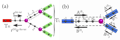
Figure 1: (Color online) (a) The schematic figure is a Cayley tree of generation $N=2$ with $N_{b}=2$ ‘small’ masses $m$ on each branch. The basic unit, is indicated with a dashed square and it consists of a branch and a vertex attached to the right end of the branch. A monochromatic incident wave $e^{ikz-i\omega t}$ is reflected back as $r^{(N)}e^{-ikz-i\omega t}$, where $r^{(N)}$ is the total reflection amplitude. For the study of thermal transport, the Cayley tree is connected to two heat baths at different temperatures, $T_{H}$ and $T_{L}$ respectively. The reservoirs consist of harmonic one-dimensional atomic chains and are assumed to be in equilibrium. (b) A scattering process occurring at a basic unit associated with the $l$th vertex. The basic unit is connected to three semi-infinite leads (blue boxes). Three incoming waves from the leads are transformed to three outgoing waves at each of the leads attached to the basic unit.

In the present paper we study heat current and its thermal fluctuations in a class of harmonic mass networks which are topologically equivalent to Cayley trees. This class of networks does not include any closed loops and has been extensively used in various areas of physics MP ; B82 . A phononic Cayley tree consists of vertices (branching points) and branches in which the metric information is introduced. To be specific, each branch is an one-dimensional chain consisting of $N_{b}$ equal masses $m$ and $(N_{b}+1)$ springs with the same equilibrium length and spring constant $\kappa$. The vertices are occupied by masses $M$. The tree is characterized by its connectivity $Z$ (number of branches emanating from a vertex) or equivalently by the associated branching number $K=Z-1$, and its generation $N$ (number of branching repetition). For each generation $N$, the total number of vertices and branches are $(K^{N}-1)/(K-1)$. We will consider trees with $Z=3$ which are connected to two heat baths $H$ and $L$ kept at temperatures $T_{H},T_{L}$ respectively with $T_{H}>T_{L}$. The bath $H$ consists of one-dimensional semi-infinite spring chain of equal masses $m$ coupled together with spring constants $\kappa$. The bath $L$ contains $K^{N}$ similar one-dimensional semi-infinite spring chains. An example of a Cayley tree for $N=2$ and $N_{b}=2$ is shown in Fig.1(a). We find that in the large $N\rightarrow\infty$ limit the transmittance, as a function of frequency of the incident wave, exhibits stop bands (total reflection) and pass bands (only partial reflection). A direct consequence is that both the heat current ${\cal I}_{\infty}$ and its thermal fluctuations $\Delta$ acquire some constant value thus reflecting the ballistic nature of the heat transport in such trees. Furthermore we show that, due to impedance mismatch phenomena, they are non-monotonic functions of the mass ratio $\mu=M/m$: they get their maxima at $\mu\sim 1$ while increasing/decreasing $\mu$ leads to a decrease of their value. In particular, there are cases where both heat current and its fluctuations are strictly zero below some critical value $\mu^{*}$. Our analysis below applies equally well to Cayley trees with and without an on-site pinning potential $\kappa_{0}$.

Theoretical Formalism -Formally, the steady-state thermal current for the Cayley tree is obtained by using the Landauer-like formula D08

$${\cal I}= \int_{0}^{\infty}\frac{\mathrm{d}\omega}{2\pi}\hbar\omega{\cal T}\left(\omega\right)\left(f_{H}\left(\omega\right)-f_{L}\left(\omega\right)\right),$$ (1)

with $f_{\alpha}=\left\{\exp\left(\hbar\omega/k_{B}T_{\alpha}\right)-1\right\}^{-1}$ being the Bose-Einstein distribution for the heat bath $\alpha=H,\>L$ and ${\cal T}(\omega)$ is the transmittance. The latter can be expressed via the total reflection amplitude $r(\omega)$ to the left reservoir as ${\cal T}(\omega)=1-|r(\omega)|^{2}$. The simplicity of the Cayley tree set-up permits us to express the full counting statistics (FCS) in terms of ${\cal T}(\omega)$. The associated steady-state cumulant generating function $\mbox{ln}Z\left(\xi\right)\equiv\mbox{ln}\left\langle e^{i\xi Q}\right\rangle$ is Li2012

$$\lim_{t_{M}\rightarrow\infty} \frac{\mbox{ln}Z\left(\xi\right)}{t_{M}}=-\int_{0}^{\infty}\frac{\mathrm{d}\omega}{2\pi}\mbox{ln}\left\{1-\mathcal{T}\left(\omega\right)F\left(\omega\right)\right\},$$ (2)

where $F\left(\omega\right)=\left(e^{i\xi\hbar\omega}-1\right)f_{H}\left(1+f_{L}\right)+\left(e^{-i\xi\hbar\omega}-1\right)f_{L}\left(1+f_{H}\right)$. The random variable $Q$ defines the total amount of heat flowing out of the heat bath $H$ during the time $t_{M}$. Note that the steady- state thermal current Eq. (1) is related to the first cumulant of $Q$ as ${\cal I}=\lim_{t_{M}\rightarrow\infty}\langle Q\rangle/t_{M}$. Likewise, the second cumulant gives the current noise

$$\Delta\equiv\frac{\left\langle\left(\Delta Q\right)^{2}\right\rangle}{t_{M}}= \int_{0}^{\infty}\frac{\mathrm{d}\omega}{2\pi}\left(\hbar\omega\right)^{2}\{\left(f_{H}+f_{L}+2f_{H}f_{L}\right)\mathcal{T}\left(\omega\right)$$

$$+\left(f_{H}-f_{L}\right)^{2}\mathcal{T}^{2}\left(\omega\right)\}.$$ (3)

Thus the analysis of the FCS of heat current in a Cayley tree reduces to the study of the transmittance $\mathcal{T}\left(\omega\right)$.

Transmission Coefficient - The analysis of the transmission coefficient of the Cayley-tree is best carried out using a wave-scattering approach S83 ; Ch90 .

We first derive the scattering matrix for a basic scattering unit. The latter consists of a mass $M$ placed at a generic vertex $l$ and $N_{b}$ masses $m$ associated with a branch attached to the left of the vertex (see Fig. 1a). The equilibrium position of the $j$-th mass is $z_{j}=aj$ where $a$ is the equilibrium distance between consequent masses and $j=1,\cdots,\left(N_{b}+1\right)$. Below we set $a=1$. The vertex $l$ is placed at the right end of the branch at $j=N_{b}+1$. The scattering problem associated with the basic unit is defined by attaching one semi-infinite lead with masses $m$ at the left end of the branch and two other identical semi-infinite leads extended at the right of the $l$-th vertex. The distance $z_{j}$ at the leads is always measured from left to right (see Fig 1b). The displacement of any of these masses can be expressed in terms of two counter-propagating waves

$$u_{n}^{(l,j)}=\left(A_{n}^{(l)}e^{ikz_{j}}+B_{n}^{(l)}e^{-ikz_{j}}\right)e^{-i\omega t},$$ (4)

where the subindex $n=1$ indicates the branch and the associated left lead and $n=2,3$ the remaining two leads extended to the right of the vertex $l$. The frequencies $\omega$ are given by the dispersion relation $\omega=\sqrt{\frac{2\kappa}{m}\left(1-\cos k\right)+\frac{\kappa_{0}}{m}}$, with $k\in[0,\pi]$, so that the propagating waves Eq. (4) satisfy the equations of motion for the masses $m$ at the branch and leads note1 . Furthermore Eq. (4) has to satisfy a consistency relation at the vertex:

$$u_{1}^{(l,N_{b}+1)}=u_{2}^{(l,0)};\quad u_{1}^{(l,N_{b}+1)}=u_{3}^{(l,0)}$$ (5)

together with the equation of motion for the mass $M$

$$M{\ddot{u}}_{2}^{(l,0)}=\kappa(u_{2}^{(l,1)}-3u_{2}^{(l,0)}+u_{3}^{(l,1)}+u_{1}^{(l,N_{b})})-\kappa_{0}u_{2}^{(l,0)}$$ (6)

Substituting into Eqs. (5,6) the expressions Eq. (4) we find the basic unit scattering matrix $S^{(l)}$ which connects incoming to outgoing waves as $(B_{1}^{(l)},A_{2}^{(l)},A_{3}^{(l)})^{T}=S^{(l)}(A_{1}^{(l)},B_{2}^{(l)},B_{3}^{(l)})^{T}$:

$$S^{(l)}= \frac{1}{3+iF}\begin{bmatrix}-(1+iF)e^{2i\alpha}&2e^{i\alpha}&2e^{i\alpha}\\ 2e^{i\alpha}&-\left(1+iF\right)&2\\ 2e^{i\alpha}&2&-\left(1+iF\right)\end{bmatrix},$$ (7)

where $F=\left(3-2\mu\right)\tan\frac{k}{2}+\frac{\kappa_{0}\left(1-\mu\right)}{\sin k}$, and $\alpha=k\left(1+N_{b}\right)$ accounts for the accumulated phase due to the wave propagation through the branch $n=1$. The scattering matrix $S^{(l)}$ satisfies the unitarity condition $(S^{(l)})^{\dagger}S^{(l)}=I$ and the time-reversal symmetry constrain $(S^{(l)})^{T}=S^{(l)}$.

Next, we build up a tree from many scattering units and calculate the total reflection amplitude to the left lead. To this end we connect two trees of $N$-generation, with identical reflection amplitudes $r^{(N)}$, into a single tree of $(N+1)$-generation. This is done with the help of a single vertex with scattering matrix $S^{(l)}$ Eq. (7). The reflection amplitude $r^{(N+1)}$ of the $(N+1)$ generation tree can be calculated in terms of the reflection amplitudes $r^{(N)}$ and the matrix $S^{(l)}$ which connects incoming to outgoing waves. Then, using the relations $B_{1}^{(l)}\equiv r^{\left(\mathrm{N}+1\right)}A_{1}^{(l)},\>A_{2}^{(l)}\equiv\frac{B_{2}^{(l)}}{r^{\left(\mathrm{N}\right)}},\>A_{3}^{(l)}\equiv\frac{B_{3}^{(l)}}{r^{\left(\mathrm{N}\right)}}$ we establish the following recursion relation

$$r^{\left(\mathrm{N}+1\right)}=x\frac{(3-iF)r^{\left(\mathrm{N}\right)}-1-iF}{3+iF-(1-iF)r^{\left(\mathrm{N}\right)}},\,r^{(1)}=-x\frac{1+iF}{3+iF}$$ (8)

where $x=e^{2i\alpha}$. The initial condition $r^{(1)}=S_{11}^{(l)}$ is provided by Eq. (7). From Eq. (8) we get

$$r^{\left(\mathrm{N}\right)}= \frac{2x\left(-i+F\right)}{\left(\frac{2}{-1+Y^{\mathrm{N}}}+1\right)U-(x+1)F-3i(x-1)},$$ (9)

where $U(\omega)=\pm\sqrt{2y}e^{i\alpha}$, $y(\omega)=\left(F^{2}-9\right)\cos 2\alpha-6F\sin\left(2\alpha\right)-F^{2}+7$ and $Y(U)=1/Y\left(-U\right)=\frac{U+F(x-1)+3i(x+1)}{-U+F(x-1)+3i(x+1)}$. The last relation can be used to show that $r^{\left(\mathrm{N}\right)}$ is insensitive to the choice of sign $\pm$ in $U$.

When $y<0$ the modulus of $Y$ is different from unity and Eq. (9) converges to a fixed point $r^{*}$ with $|r^{*}|=1$ for $\mathrm{N}\rightarrow\infty$. In contrast, when $y>0$ we have $|Y|=1$ and Eq. (9), does not converge. We conclude therefore that the convergence of the reflection amplitude $r^{(N)}$ is determined by the sign of the band-gap parameter $y$.

In the frequency domain for which Eq. (9) converges, i.e. $y<0$, we have $\mathcal{T}^{\left(\mathrm{N\rightarrow\infty}\right)}=0$. We refer to this frequency domain as Stop Bands (SB). The situation is more complicated in the frequency domain for which $y>0$. In this case $Y$ is unimodular and thus it can be written as $Y=e^{i\varphi}$. Substituting back into Eq. (9) we obtain the following expression for the transmittance

$$\mathcal{T}^{\left(\mathrm{N}\right)}=\frac{y}{y-\left(1+F^{2}\right)\left(1-\cos\left(\mathrm{N}\varphi\right)\right)}$$ (10)

which fluctuates between a maximum value $\mathcal{T}_{max}=1$ and a minimum value $\mathcal{T}_{min}=1-\frac{1+F^{2}}{\left(F\cos\alpha-3\sin\alpha\right)^{2}}$ which is independent of the generation number $N$. We refer to the frequency domain for which $y>0$ as Pass Bands (PB). Within each PB we define a smoothed version of transmittance as

$$\overline{\mathcal{T}}\equiv\frac{\mathcal{T}_{min}+\mathcal{T}_{max}}{2}=1-\frac{1+F^{2}}{2\left(F\cos\alpha-3\sin\alpha\right)^{2}},$$ (11)

while within the SB we can approximate the transmittance with its asymptotic value i.e. $\overline{\cal T}=0$. We will see below that these approximations describe well our numerical results for the heat current and its fluctuations in the limit $N\rightarrow\infty$. The transition points between a PB and a SB correspond to frequencies for which $y(\omega)=0$.

In Fig. 2 we present two typical transmission spectra for a Cayley tree network of $N=3$ and $N=8$. We see that they consist of alternating SB and PB as the wave number $k$ changes from $0$ to $\pi$. Armed with the knowledge about the transmittance of a Cayley tree we are now ready to investigate the heat current and its fluctuations Eqs. (1,3).

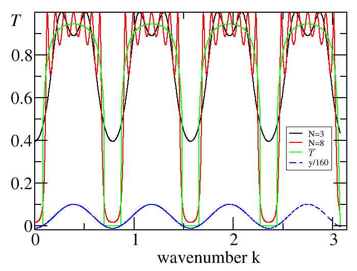
Figure 2: (Color online) Transmittance $\mathcal{T}^{(N)}=1-|r^{(N)}|^{2}$ vs wave number $k$ for various $N$-values obtained using Eq. (9). For comparison, we also plot the mean value approximation $\overline{\cal T}$ and the band-gap parameter $y$ (scaled by 160 to fit the figure). Here $m=1$, $\kappa=1$, $\mu=1.5$, $\kappa_{0}=0$ and $N_{b}=3$.

Heat Current and its fluctuations - First we consider the scaling of the steady-state thermal current ${\cal I}_{N}$, calculated using Eq. (1), with respect to the tree generation $N$. A detailed scaling analysis indicates that ${\cal I}_{N}$ converges to its asymptotic value exponentially fast i.e. ${\cal I}_{N}-{\cal I}_{N\rightarrow\infty}\sim\exp(-\gamma N)$ (see inset of Fig. 3a). Below we will be using $N=50$ as a good approximation for the asymptotic heat current ${\cal I}_{\infty}$.

In the main panels of Fig. 3 we report the dependence of ${\cal I}_{\infty}$ and its fluctuations $\Delta$, Eqs. (1,3), on the mass ratio $\mu=M/m$ for two representative values of the number of masses $N_{b}=0,3$ at the branches. The solid lines in these figures correspond to the numerical results obtained from Eq. (9). For comparison we plot the theoretical predictions (symbols) associated with the approximated expression for the transmittance $\overline{\cal T}(\omega)$ given in Eq. (11).

Generally, the asymptotic value ${\cal I}_{\infty}$ is nonzero, reflecting the ballistic nature of the thermal transport across a Cayley tree. We find that ${\cal I}_{\infty}$ is a non-monotonic function of the mass ratio $\mu$. Indeed, in the two limiting cases of $\mu\ll 1$ and $\mu\gg 1$ there is a considerable impedance miss-matching between the masses $m$ of the leads attached to the reservoirs and the mass $M$ at the vertices. This impedance miss-match is, in turn, responsible for the reflection of the energy flowing from the lead to the tree and thus for the decrease of the heat current. As the mass ratio $\mu$ approaches unity the impedance matching is restored and heat current flows from the hot reservoir towards the cold reservoirs via the Cayley tree.

Although the $N_{b}=3$ case is representative of the dependence of heat current on $\mu$, the $N_{b}=0$ case shows some non-generic features. Specifically, we find that ${\cal I}_{\infty}$ vanishes for a restricted parameter range $0\leq\mu\leq\mu^{*}$. The critical value of the mass ratio can be evaluated exactly once we take into consideration the band-gap structure of the transmittance spectrum ${\cal T}(\omega)$. Specifically for $N_{b}=0$, we find that $y(\omega)<0$, for any $\omega$ given by the dispersion relation as long as

$$\mu\leq\mu^{*}=\frac{\left(3-2\sqrt{2}\right)\kappa+\kappa_{0}}{4\kappa+\kappa_{0}}.$$ (12)

In this case we only have a SB with ${\cal T}(\omega)=0$ and thus ${\cal I}_{\infty}=0$. For Cayley trees with $N_{b}\neq 0$, the band-gap parameter $y(\omega)$ changes sign at least once as the wave number varies in the interval $[0,\pi]$. Therefore the asymptotic current is different from zero for any finite $\mu$.

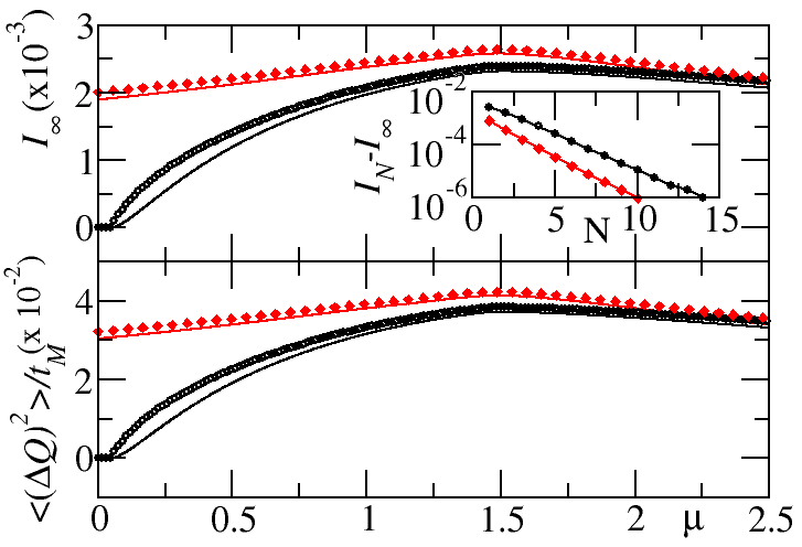
Figure 3: (Color online) (a) The steady-state thermal current ${\cal I}\left[\hbar\frac{\kappa}{m}\right]$ versus the mass ratio $\mu$ for $N_{b}=0$ (black line), and $N_{b}=3$ (red line). We have used Eq. (1) where the total transmittance has been calculated numerically using Eq. (9) for $N=50$. Black circles and red diamonds indicate the theoretical results for $N_{b}=0$ and $N_{b}=3$ when we use the mean value approximation for the transmittance. Inset: The exponential convergence of ${\cal I}$ with generation $N$ to its asymptotic value ${\cal I}_{\infty}$.Two typical cases with $\mu=0.05$ for the $N_{b}=0$ (black line) and $N_{b}=3$ (red line). (b) The same as in (a) but now for the thermal fluctuations $\Delta$. The parameters used are $T_{H}=0.41\,\frac{\hbar}{k_{B}}\sqrt{\frac{\kappa}{m}}$, $T_{R}=0.39\,\frac{\hbar}{k_{B}}\sqrt{\frac{\kappa}{m}},$ $\kappa_{0}=0$.

Finally, as an example, we report in Fig. 4 the temperature-dependence of the asymptotic conductance $\sigma^{(N\rightarrow\infty)}\equiv\lim_{T_{H}\rightarrow T_{L}}{\cal I}(T_{H},T_{L})/(T_{H}-T_{L})$ for $\kappa_{0}=0$ and $\mu=\frac{3}{2}$. In the high-temperature limit, the asymptotic current approaches its classical value leading to a saturation of the conductance. It is thus instructive to calculate the classical limit of ${\cal I}_{\infty}$. In this case the Landauer-like formula Eq. (1) reduces to

$${\cal I}_{\infty}^{Cl}= \int_{0}^{\infty}\frac{\mathrm{d}\omega}{2\pi}\mathcal{T}\left[\omega\right]k_{B}\left(T_{H}-T_{L}\right)$$ (13)

which can be analytically evaluated using the mean value approximation for the transmittance Eq. (11) within the PB frequency range. The PBs frequency range can be obtained from the analysis of the band-gap parameter $y$. The corresponding wave-numbers take values in the interval $k\in\left[\frac{\arccos\frac{7}{9}+2\pi n}{2\left(N_{b}+1\right)},\>\frac{2\pi\left(n+1\right)-\arccos\frac{7}{9}}{2\left(N_{b}+1\right)}\right]$ for $n=0,\,1,\ldots,N_{b}$. The resulting expression for the classical current is then

$$I_{\infty}^{Cl}= \frac{k_{B}\sqrt{\kappa}}{\pi\sqrt{m}}\frac{\sin\left(\frac{\delta}{4\left(N_{b}+1\right)}\right)}{\sin\left(\frac{\pi}{4\left(N_{b}+1\right)}\right)}\mathcal{\overline{T}}\Delta T\xrightarrow{N_{b}\rightarrow\infty}\frac{k_{B}\sqrt{\kappa}\delta}{\sqrt{m}\pi^{2}}\mathcal{\overline{T}}\Delta T$$ (14)

where $\delta=\pi-\arccos\frac{7}{9}$ and $\Delta T=T_{H}-T_{L}$. In Eq. (14) we have used the additional simplification that $\overline{\cal T}$ is nearly a constant in all PBs.

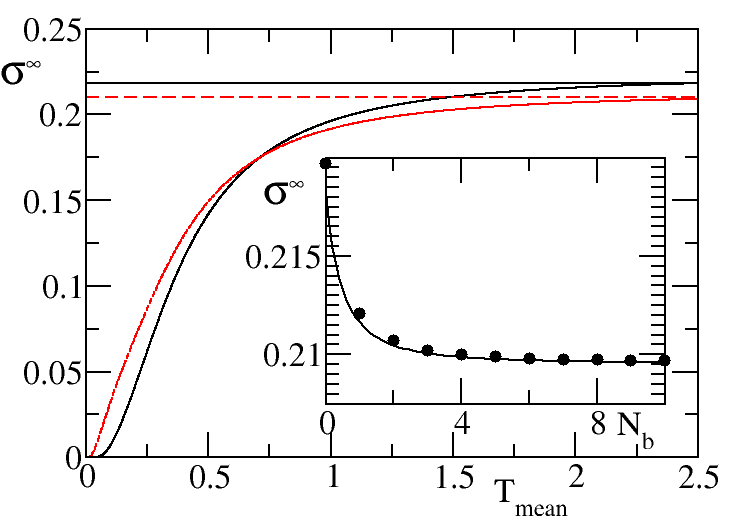
Figure 4: (Color online) Numerical values of conductance $\sigma^{\infty}\left[k_{B}\sqrt{\frac{\kappa}{m}}\right]$ versus temperature $T_{\rm mean}=(T_{H}+T_{L})/2$ $\left[\frac{\hbar}{k_{B}}\sqrt{\frac{\kappa}{m}}\right]$ for $N_{b}=0$ (black solid line) and $N_{b}=3$ (red dashed line). The horizontal lines (of the same type and color) are the classical results of Eq. (14). Inset: Numerical values (black circles) and classical values Eq. (14) (solid black line) of conductance versus $N_{b}$. The numerical results corresponds to $N=50$ and we have used Eq. (1) where the total transmittance has been calculated using Eq. (9). Other parameters are $\mu=1.5$, $\kappa_{0}=0$. For the inset we have used $T_{\rm mean}=3\left[\frac{\hbar}{k_{B}}\sqrt{\frac{\kappa}{m}}\right]$.

I Conclusion

We study heat transport through a Cayley tree. The tree is built out of masses $M$ (vertices) connected by branches which consist of masses $m$ linked by identical springs. First we calculated transmission of phonon waves through the tree and show that, depending on the frequency, waves are either totally reflected (stop band) or get partially transmitted (pass band). Then we studied the heat current through the structure and show that, in the limit of an infinite tree, both the average current and its variance approach a well defined limit which, in some particular cases, can be strictly zero.

References

- (1) S. Lepri, R. Livi, A. Politi, Phys. Rep. 377, 1 (2003).
- (2) A. Dhar, Adv. Phys. 57, 457 (2008).
- (3) C. W. Chang, D. Okawa, H. Garcia, A. Majumdar, and A. Zettl, Phys. Rev. Lett, 101, 075903 (2008).
- (4) D. L. Nika, S. Ghosh, E. P. Pokatilov, and A. A. Balandin, Appl. Phys. Lett. 94, 203103 (2009).
- (5) N. Li, J. Ren, L. Wang, G. Zhang, P. Hänggi, and B. Li, Rev. Mod. Phys. 84, 1045 (2012).
- (6) G. Zhang, B. Li, NanoScale 2, 1058 (2010).
- (7) S. Lepri, R. Livi, A. Politi, Phys. Rev. Lett. 78, 1896 (1997)
- (8) B. Li, G. Casati, J. Wang, T. Prosen, Phys. Rev. Lett. 92, 254301 (2004).
- (9) Tomaz Prosen and David K. Campbell, Chaos 15, 015117 (2005)
- (10) A. Dhar, Phys. Rev. Lett. 86, 5882 (2001).
- (11) A. V. Savin and Y. A. Kosevich, Phys. Rev. E 89, 032102 (2014).
- (12) K. Saito, A. Dhar, Phys. Rev. Lett. 99, 180601 (2007); Phys. Rev. E 83, 041121 (2011).
- (13) J. Ren, P. Hanggi, and B. Li, Phys. Rev. Lett. 104, 170601 (2010).
- (14) M. Schmidt, T. Kottos, B. Shapiro, Phys. Rev. E 88, 022126 (2013).
- (15) Diller K R (ed) 1998 Biotransport: Heat and Mass Transfer in Living Systems (New York: Academy of Sciences)
- (16) L. Hu L, D. S. Hecht, and G. Gruner, Nano Lett. 4, 2513 (2004); D. S. Hecht, L. Hu and G. Gruner, Appl. Phys. Lett. 89, 133112 (2006).
- (17) S. Kumar, J. Y. Murthy, M. A. Alam M A, Phys. Rev. Lett. 95, 066802 (2005).
- (18) C. W. Chang, D. Okawa, A. Majumdar and A. Zettl, Science 314, 1121 (2006); C. W. Chang, D. Okawa, H. Garcia, A. Majumdar and A. Zettl, Phys. Rev. Lett. 101, 075903 (2008).
- (19) E. Pop, D. Mann, J. Cao, Q. Wang, K. Goodson, and H. Dai, Phys. Rev. Lett. 95, 155505 (2005)
- (20) B. Shapiro, Phys. Rev. Lett. 50, 747 (1983).
- (21) J. T. Chalker and S. Siak, J. Phys. Condens. Matter 2, 2671 (1990).
- (22) M. Ostilli, Cayley Trees and Bethe Lattices, a concise analysis for mathematicians and physicists, Physica A 391, 3417 (2012).
- (23) R. J. Baxter, Exact Solved Models in Statistical Mechanics (Academic Press, London, 1982).
- (24) H. Li, B. K. Agarwalla, and J.-S. Wang, Phys. Rev. B 86, 165425 (2012).
- (25) E. N. Economou Green’s Functions in Quantum Physics, Springer Series in Solid State Sciences (1990).
- (26) M. Eckstein, M. Kollar, K. Byczuk, and D. Vollhardt, Phys. Rev. B 71, 235119 (2005).
- (27) We note that for the special case , the branches does not contain any small mass ‘’ and the prescribed dispersion relation is simply an ansatz for a unified treatment, which will be justified by introducing the branch-dependent amplitudes to satisfy all the required equations of motion.