Strong convergence for split-step methods in stochastic jump kinetics

Abstract.

Mesoscopic models in the reaction-diffusion framework have gained recognition as a viable approach to describing chemical processes in cell biology. The resulting computational problem is a continuous-time Markov chain on a discrete and typically very large state space. Due to the many temporal and spatial scales involved many different types of computationally more effective multiscale models have been proposed, typically coupling different types of descriptions within the Markov chain framework.

In this work we look at the strong convergence properties of the basic first order Strang, or Lie-Trotter, split-step method, which is formed by decoupling the dynamics in finite time-steps. Thanks to its simplicity and flexibility, this approach has been tried in many different combinations.

We develop explicit sufficient conditions for path-wise well-posedness and convergence of the method, including error estimates, and we illustrate our findings with numerical examples. In doing so, we also suggest a certain partition of unity representation for the split-step method, which in turn implies a concrete simulation algorithm under which trajectories may be compared in a path-wise sense.

1. Introduction

Since their introduction by Gillespie [21, 22], stochastic models of chemical reactions have become ubiquitous tools in describing the kinetics of living cells. Since complete Molecular Dynamics-type descriptions of most biochemical processes are either impractical or out of reach for complexity reasons, stochastic models have remained popular as a viable alternative. Formulated in a way which resembles the macroscopic viewpoint, but with randomness taking certain microscopic effects into account, mesoscopic stochastic models attempt to strike a balance between computational feasibility and accuracy. In fact, a common theme in several studies is the discrepancy between deterministic and stochastic descriptions [6, 31, 38].

Due to the presence of multiple scales in species abundance and in reaction rates, the computational problem of simulating well-stirred or spatially extended models has caught a lot of attention. For example, these features are the driving motivation behind the development of hybrid methods [25, 5] and the various kinds of model reduction techniques that have been proposed [24, 12, 14, 17]. Similarly, more efficient time discretization “tau-leap” methods were proposed early on [23], and has since then been modified and analyzed in various ways [1, 30, 34].

As a means to facilitate multiscale- and multiphysics coupling in method’s development in general, split-step methods have a long story. Originally developed via (finite-dimensional) operator splitting [37], in the present case these methods became particularly important in the more computationally demanding spatial stochastic reaction-diffusion setting [16]. An analysis in the sense of convergence in distribution in the master equation setting was presented in [27]. A practical method based on splitting to simulate fractional diffusion was reported in [8], and an adaptive reaction-diffusion simulator was suggested in [26]. Finally, in [4], the splitting technique was used to bring out parallelism from an otherwise strictly serial description.

In this work we look at the strong path-wise convergence of the basic first order (in the operator sense) split-step method. A key issue here is to devise a meaningful coupling between different trajectories conditioned on different split-step discretizations. We solve this by using a partition of unity representation which as a by-product also implies a practical algorithm. Sufficient conditions for strong convergence of order $1/2$ that apply notably also to open chemical systems are described and this is also confirmed in our numerical experiments. An interesting observation is that, although still only formally of strong order $1/2$, the second order (again in the operator sense) Strang splitting performs considerably better than the first order splitting.

In §2 we recapitulate the description of chemical processes as continuous-time Markov chains, in the non-spatial as well as in the spatially extended case. Our main theoretical findings, including explicit conditions for strong convergence, are reported in §3. Numerical illustrations are presented in §4, and a concluding discussion is found in §5.

2. Stochastic jump kinetics

We summarize in this section the mathematical background required in the description of biochemical processes. A recapitulation of the traditional well-stirred setting is found in §2.1. Path-wise descriptions are found in §2.2, where some fundamental tools from stochastic analysis are also reviewed. Finally, in §2.3 the required extensions to encompass also spatially extended models are indicated.

2.1. Well-stirred Markovian reactions

In a memory-less Markovian chemical system, at any instant $t$, the state is an integer vector $X(t)\in\mathbf{Z}_{+}^{D}$ counting the number of molecules of each of $D$ species. The reactions are prescribed transitions of the state according to an intensity law, or reaction propensity;

(2.1) $$w_{r}:\mathbf{Z}_{+}^{D}\to\mathbf{R}_{+},$$

(2.2) $$\mathbf{P}\left[X(t+dt)=x-\mathbb{N}_{r}|\;X(t)=x\right] =w_{r}(x)\,dt+o(dt).$$

The system is thus fully described by the pair $[\mathbb{N},w(x)]$, that is, the stoichiometric matrix $\mathbb{N}\in\mathbf{Z}^{D\times R}$, and $w(x)\equiv[w_{1}(x),\ldots,w_{R}(x)]^{T}$, the column vector of reaction propensities. An important remark is that useful physical descriptions are always conservative, for all propensities it holds that $w_{r}(x)=0$ whenever $x-\mathbb{N}_{r}\not\in\mathbf{Z}_{+}^{D}$ [10, Chap. 8.2.2, Definition 2.4].

The chemical master equation (CME) [28, Chap. V], or Kolmogorov’s forward differential system [10, Chap. 8.3] governs the law of the state $X(t)$ conditioned on some initial state. Put $p(x,t)=\mathbf{P}(X(t)=x|\;X(0)=x_{0})$. Then

(2.3) $$\frac{\partial p(x,t)}{\partial t} =\sum_{r=1}^{R}w_{r}(x+\mathbb{N}_{r})p(x+\mathbb{N}_{r},t)-w_{r}(x)p(x,t)=:\mathbb{M}^{T}p(x,t),$$

where $\mathbb{M}$ is the infinitesimal generator of the process.

2.2. Path-wise representations

The use of path-wise representations in the analysis of Markov processes on discrete state-spaces in continuous time was pioneered by Kurtz in a series of paper (see [18] and the references therein). We thus postulate the probability space $(\Omega,\mathcal{F},\mathbf{P})$, where the filtration $\mathcal{F}_{t\geq 0}$ contains $R$-dimensional Poisson processes. The transition law (2.2) implies a certain counting process which can be constructed from a standard unit-rate Poisson process $\Pi_{r}$. The state $X(t)$ can then be written

(2.4) $$X_{t} =X_{0}-\sum_{r=1}^{R}\mathbb{N}_{r}\Pi_{r}\left(\int_{0}^{t}w_{r}(X_{s-})\,ds\right).$$

This is Kurtz’s random time change representation [18, Chap. 6.2] which gives rise to the notion of operational time in the argument to each of the $R$ independent Poisson processes. Note that, in (2.4), by $X(t-)$ is meant the state before any transitions at time $t$.

It is sometimes convenient to use an equivalent construction in terms of a random counting measure [9, Chap. VIII]. We denote by $\mu_{r}(dt)=\mu_{r}(w_{r}(X_{t-})\,dt;\,\omega)$ for $\omega\in\Omega$ the random measure associated with the counting process whose intensity at any instant $t$ is $w_{r}(X_{t-})$. Thus with deterministic intensity $\operatorname{E}[\mu_{r}(dt)]=\operatorname{E}[w_{r}(X_{t-})\,dt]$, this defines an increasing sequence of exponentially distributed counts $\tau_{i}\in\mathbf{R}_{+}$. With $\boldsymbol{\mu}=[\mu_{1},\ldots,\mu_{R}]^{T}$ we can now write (2.4) in the compact differential form

(2.5) $$dX_{t} =-\mathbb{N}\boldsymbol{\mu}(dt).$$

For realistic chemical systems the number of molecules must somehow be bound a priori. We encapsulate this property by requiring the existence of a certain weighted norm

(2.6) $$\left\|x\right\|_{\boldsymbol{l}}:=\boldsymbol{l}^{T}x,\quad x\in\mathbf{Z}_{+}^{D},$$

normalized such that $\min_{i}\boldsymbol{l}_{i}=1$. Equipped with this norm we formulate, following [15] closely (see also [11, 33]),

Assumption 2.1.

For arguments $x$, $y\in\mathbf{Z}_{+}^{D}$ we assume that

1. $-\boldsymbol{l}^{T}\mathbb{N}w(x)\leq A+\alpha\left\|x\right\|_{\boldsymbol{l}}$,

2. $(-\boldsymbol{l}^{T}\mathbb{N})^{2}w(x)/2\leq B+\beta_{1}\left\|x\right\|_{\boldsymbol{l}}+\beta_{2}\left\|x\right\|_{\boldsymbol{l}}^{2}$,

3. $|w_{r}(x)-w_{r}(y)|\leq L_{r}(P)\|x-y\|$, for $r=1,\ldots,R$, and $\left\|x\right\|_{\boldsymbol{l}}\vee\left\|y\right\|_{\boldsymbol{l}}\leq P$.

With the exception of $\alpha$, all parameters $\{A,B,\beta_{1},\beta_{2},L\}$ are assumed to be non-negative.

In order to state an a priori result concerning the regularity of the solutions to (2.5), following [36, Sect. 3.1.2], we define the following family of spaces of path-wise locally bounded processes:

(2.9) $$S_{\mathcal{F}}^{p,\mathrm{loc}}(\mathbf{Z}_{+}^{D}) =\left\{X(t,\omega):\begin{array}[]{l}X_{t}\in\mathbf{Z}_{+}^{D}\mbox{ is $\mathcal{F}_{t}$-adapted such that }\\ \operatorname{E}\,\sup_{t\in[0,T]}\left\|X_{t}\right\|_{\boldsymbol{l}}^{p}<\infty\mbox{ for }\forall T<\infty\end{array}\right\}.$$

Theorem 2.1 (Theorem 4.7 in [15]).

Let $X_{t}$ be a solution to (2.5) under Assumption 2.1 (i) and (ii) with $\beta_{2}=0$. Then if $\left\|X_{0}\right\|_{\boldsymbol{l}}^{p}<\infty$, $\{X_{t}\}_{t\geq 0}\in S_{\mathcal{F}}^{p,\mathrm{loc}}(\mathbf{Z}_{+}^{D})$. If $\beta_{2}>0$ then the conclusion remains under the additional requirement that $\left\|X_{0}\right\|_{\boldsymbol{l}}^{p+1}<\infty$.

Below we will frequently use the stopping time

(2.10) $$\tau_{P}:=\inf_{t\geq 0}\{\left\|X_{t}\right\|_{\boldsymbol{l}}>P\}$$

and put $\hat{t}=t\wedge\tau_{P}$ for some finite $t$ defining an interval of interest. As an example, a differential form of Itô’s change of variables formula can be derived formally by simply summing over jump times [3, Chap. 4.4.2]

(2.11) $$df(X_{t}) =\sum_{r=1}^{R}f(X_{t-}-\mathbb{N}_{r})-f(X_{t-})\,\mu_{r}(dt).$$

More carefully, Dynkin’s formula for the stopped process is then given by [10, Chap. 9.2.2],

(2.12) $$\operatorname{E}f(X_{\hat{t}})-\operatorname{E}f(X_{0}) =\int_{0}^{\hat{t}}\sum_{r=1}^{R}\operatorname{E}\left[(f(X_{s}-\mathbb{N}_{r})-f(X_{s}))w_{r}(X_{s})\right]\,ds.$$

In order to efficiently work with the Poisson representation (2.4) in the sense of mean square, the following two lemmas which follows [13, Manuscript] very closely will be critical.

Lemma 2.2.

Let $\Pi$ be a unit-rate Poisson process and $T$ a bounded stopping time, both adapted to $\mathcal{F}_{t}$. Then

(2.13) $$\operatorname{E}[\Pi(T)] =\operatorname{E}[T],$$

(2.14) $$\operatorname{E}[\Pi^{2}(T)] =2\operatorname{E}[\Pi(T)T]-\operatorname{E}[T^{2}]+\operatorname{E}[T].$$

Proof.

Let $\tilde{\Pi}(t):=\Pi(t)-t$ be the compensated process. This is a martingale and Doob’s optional sampling theorem implies $\operatorname{E}[\tilde{\Pi}(T)]=0$ [32, Theorem 17, Chap. I.2], which is (2.13). Similarly $Z(t):=\tilde{\Pi}^{2}(t)-t$ is a martingale [32, Theorem 24, Chap. I.3] and the sampling theorem yields $\operatorname{E}[Z(T)]=0$, or,

$$0 =\operatorname{E}[\Pi^{2}(T)-2\Pi(T)T+T^{2}-T],$$

which is (2.14). ∎

Lemma 2.3.

Let $\Pi$ be a unit-rate Poisson process and $T_{1}$, $T_{2}$ bounded stopping times, all adapted to $\mathcal{F}_{t}$. Then

(2.15) $$\operatorname{E}[|\Pi(T_{2})-\Pi(T_{1})|] =\operatorname{E}[|T_{2}-T_{1}|],$$

(2.16) $$\operatorname{E}[(\Pi(T_{2})-\Pi(T_{1}))^{2}] =2\operatorname{E}[|\Pi(T_{2})-\Pi(T_{1})|(T_{1}\vee T_{2})]$$

$$\hphantom{=}-\operatorname{E}[|T_{2}^{2}-T_{1}^{2}|]+\operatorname{E}[|T_{2}-T_{1}]].$$

The formulation (2.15) was recently used in [19, Manuscript] to provide for a related analysis in the sense of convergence in mean.

Proof.

Assume first that $T_{2}\geq T_{1}$. By Lemma 2.2 (2.13),

$$\operatorname{E}[\Pi(T_{2})-\Pi(T_{1})] =\operatorname{E}[T_{2}-T_{1}].$$

For general stopping times $S_{1}$, $S_{2}$, say, (2.15) follows upon substituting $T_{1}:=S_{1}\wedge S_{2}$ and $T_{2}:=S_{1}\vee S_{2}$ into this equality.

Next put $X:=\operatorname{E}[(\Pi(T_{2})-\Pi(T_{1}))^{2}]$ and assume anew that $T_{2}\geq T_{1}$. We find

$$X =\operatorname{E}[\Pi(T_{2})^{2}+\Pi(T_{1})^{2}-2\Pi(T_{1})\Pi(T_{2})]$$

$$=\operatorname{E}[\Pi(T_{2})^{2}+\Pi(T_{1})^{2}]-2\operatorname{E}[\Pi(T_{1})\operatorname{E}[\Pi(T_{2})|\mathcal{F}_{T_{1}}]].$$

To evaluate the iterated expectation, note that

$$\operatorname{E}[\tilde{\Pi}(T_{2})|\mathcal{F}_{T_{1}}] =\tilde{\Pi}(T_{1})\Longrightarrow\operatorname{E}[\Pi(T_{2})|\mathcal{F}_{T_{1}}]=\Pi(T_{1})-T_{1}+E[T_{2}|\mathcal{F}_{T_{1}}].$$

Hence

$$\operatorname{E}[\Pi(T_{1})\operatorname{E}[\Pi(T_{2})|\mathcal{F}_{T_{1}}]] =\operatorname{E}[\Pi(T_{1})^{2}]-\operatorname{E}[\Pi(T_{1})T_{1}]+\operatorname{E}[\Pi(T_{1})T_{2}],$$

and so

$$X =\operatorname{E}[\Pi(T_{2})^{2}-\Pi(T_{1})^{2}]+2\operatorname{E}[\Pi(T_{1})T_{1}]-2\operatorname{E}[\Pi(T_{1})T_{2}].$$

Applying Lemma 2.2 (2.14) twice then yields

$$X =2\operatorname{E}[(\Pi(T_{2})-\Pi(T_{1}))T_{2}]-\operatorname{E}[T_{2}^{2}-T_{1}^{2}]+\operatorname{E}[T_{2}-T_{1}].$$

As before the substitutions $T_{1}:=S_{1}\wedge S_{2}$ and $T_{2}:=S_{1}\vee S_{2}$ implies (2.16) for general stopping times $S_{1}$, $S_{2}$. ∎

Lemma 2.3 will be applied as follows. Assuming first the a priori bound $T_{1}\vee T_{2}\leq B$ we get from (2.15)–(2.16) that

(2.17) $$\operatorname{E}[(\Pi(T_{2})-\Pi(T_{1}))^{2}] \leq(2B+1)\operatorname{E}[|T_{2}-T_{1}|].$$

Let $\mathcal{F}_{t}$ be the filtration adapted to $\{\tilde{\Pi}_{r}\}_{r=1}^{R}$. Then for any fixed time $t$, $T_{r}(t):=\int_{0}^{t}w_{r}(X(s))\,ds$ is a stopping time adapted to [2, Lemma 3.1]

$$\tilde{\mathcal{F}}^{r}_{u}:=\sigma\{\Pi_{r}(s),s\in[0,u];\;\Pi_{k\not=r}(s),s\in[0,\infty]\}.$$

Intuitively, since $X(t)=\sum_{r}\Pi_{r}(T_{r}(t))\mathbb{N}_{r}$, the event $\{T_{r}(t)<u\}$ depends on $\Pi_{r}$ during $[0,u]$ and on $\{\Pi_{k},k=1\ldots R,\,k\neq r\}$ during $[0,\infty)$. However, since $\{\Pi_{r}\}_{r=1}^{R}$ are all independent, $\tilde{\Pi}_{r}$ is still a martingale with respect to $\tilde{\mathcal{F}}^{r}_{u}$ (and not only with respect to $\mathcal{F}^{r}_{u}=\sigma\{\Pi_{r}(s),s\in[0,u]\}$). Hence we can apply the stopping time theorems to $T_{r}(t)$ and the previous lemmas apply.

For an approximating process $\tilde{X}\approx X$, say, assuming a suitable random time representation in the form of (2.4) is available, these results will remain valid for $\tilde{X}$ as well. To conclude, given the bound

(2.18) $$\int_{0}^{t}w_{r}(X(s))\,ds\vee\int_{0}^{t}\tilde{w}_{r}(\tilde{X}(s))\,ds\leq B.$$

we get from (2.17) that

$$\operatorname{E}\left[\left(\Pi_{r}\left(\int_{0}^{t}w_{r}(X(s))\,ds\right)-\Pi_{r}\left(\int_{0}^{t}\tilde{w}_{r}(\tilde{X}(s))\,ds\right)\right)^{2}\right]$$

(2.19) $$\leq(2B+1)\operatorname{E}\left[\left|\int_{0}^{t}w_{r}(X(s))\,ds-\int_{0}^{t}\tilde{w}_{r}(\tilde{X}(s))\,ds\right|\right].$$

2.3. Incorporating spatial dependence

Well-stirred modeling of chemical kinetics relies on homogeneity, that is, that the probability of finding a molecule is equal throughout the volume. There are many situations of interest where this assumption is violated, for instance, when slow molecular transport allows concentration gradients to build up. A way to approach this situation is through compartmentalization techniques [28, Chap. XIV], which leads to models with a very large number of generalized reaction channels. Since split-step methods are a particularly promising computational technique here, we briefly review this framework.

The basic premise is that, although the full volume $V$ is not well-stirred, it can be subdivided into smaller cells $V_{j}$ such that their individual volume $|V_{j}|$ is small enough that diffusion suffices to make each cell practically well-stirred.

The state of the system is thus now an array $\boldsymbol{X}\in\mathbf{Z}_{+}^{D\times K}$ consisting of $D$ chemically active species $\boldsymbol{X}_{ij}$, $i=1,\ldots,D$, in $K$ cells, $j=1,\ldots,K$. This state is changed by chemical reactions occurring in each cell (vertically in $\boldsymbol{X}$) and by diffusion where molecules move to adjacent cells (horizontally in $\boldsymbol{X}$).

Since each cell is assumed to be well-stirred, (2.5) governs the reaction dynamics,

(2.20) $$d\boldsymbol{X}_{t} =-\mathbb{N}\boldsymbol{\mu}(dt),$$

where $\boldsymbol{\mu}$ is now $R$-by-$K$ with $\operatorname{E}[\mu_{rj}]=\operatorname{E}[w_{rj}(\boldsymbol{X}_{(\cdot,j)}(t-))\,dt]$. Transport of a molecule from $V_{k}$ to $V_{j}$ can also be thought of as a special kind of reaction,

(2.21) $$\boldsymbol{X}_{ik} \xrightarrow{q_{kji}\boldsymbol{X}_{ik}}\boldsymbol{X}_{ij},$$

where the rate constant $q_{kji}$ is non-zero only for connected cells. In practice, for any given spatial discretization, numerical methods may be used to define the diffusion rates consistently [16]. We obtain from (2.21) the mesoscopic diffusion model

(2.22) $$d\boldsymbol{X}_{t} =\mathbb{S}\otimes(-\boldsymbol{\nu}^{T}+\boldsymbol{\nu})(dt),$$

where $\mathbb{S}\in\mathbf{Z}^{1\times K}$ of all 1’s, where $\boldsymbol{\nu}$ is $K$-by-$K$-by-$D$ with $\operatorname{E}[\nu_{kji}]=\operatorname{E}[q_{kji}\boldsymbol{X}_{ik}(t-)\,dt]$, and where the array operations are suitably defined. In (2.22), note how diffusion exit events are paired with entry events via the terms $-\boldsymbol{\nu}^{T}$ and $\boldsymbol{\nu}$, respectively.

By superposition of (2.20) and (2.22) we arrive at the reaction-diffusion model

(2.23) $$d\boldsymbol{X}_{t} =-\mathbb{N}\boldsymbol{\mu}(dt)+\mathbb{S}\otimes(-\boldsymbol{\nu}^{T}+\boldsymbol{\nu})(dt).$$

As was already noted in [16], part of the interest in split-step methods comes from simulating reactions and diffusions by different methods. For simplicity, in the rest of the paper we shall take the well-stirred case (2.5) as our target of study. In doing so we keep in mind that the reaction-diffusion (or reaction-transport) case (2.23) does fall under the same general class of descriptions.

3. Analysis of split-step methods

In this section we present our main theoretical findings. The splitting we choose to analyze is defined in the master equation setting in §3.1. In order to couple trajectories and obtain path-wise comparisons, the splitting is redefined in the operational time framework in §3.2, where some a priori estimates are also derived. After developing a few further preliminary results in §3.3, the theory is put together in §3.4, where our main convergence result is presented.

Throughout this section we let $C$ denote a positive constant which may be different at each occurrence.

3.1. Operator splitting and the master equation

While we take another approach below, traditionally, split-step methods are constructed via operator-splitting of the master equation (2.3). Assume the split into two sets of reaction pathways can be written as

(3.1) $$\mathbb{N} =\left[\mathbb{N}^{(1)}\;\mathbb{N}^{(2)}\right],$$

(3.2) $$w(x) =\left[w^{(1)}(x);\;w^{(2)}(x)\right],$$

where $\mathbb{N}^{(i)}$ is $D$-by-$R_{i}$, $i\in\{1,2\}$, $R_{1}+R_{2}=R$, and where the propensity column vectors have the corresponding dimensions. The simplest possible split-step method, and the one we choose to analyze in this paper, can then be written in integral form as (compare (2.3))

(3.3) $$\tilde{p}_{h}(x,t+h) =p_{h}(x,t)+\int_{t}^{t+h}\sum_{r\in\mathcal{R}_{1}}w_{r}(x+\mathbb{N}_{r})\tilde{p}_{h}(x+\mathbb{N}_{r},s)-w_{r}(x)\tilde{p}_{h}(x,s)\,ds,$$

(3.4) $$p_{h}(x,t+h) =\tilde{p}_{h}(x,t+h)+\int_{t}^{t+h}\sum_{r\in\mathcal{R}_{2}}w_{r}(x+\mathbb{N}_{r})p_{h}(x+\mathbb{N}_{r},s)-w_{r}(x)p_{h}(x,s)\,ds,$$

where $\mathcal{R}_{1}=\{1,\ldots,R_{1}\}$, $\mathcal{R}_{2}=\{R_{1}+1,\ldots,R\}$. Loosely speaking, (3.3) evolves the dynamics of the first set of reactions in an auxiliary variable $\tilde{p}_{h}$ from time $t$ to $t+h$, and (3.4) similarly evolves the second.

3.2. Splitting in operational time

To obtain a concrete path-wise formulation which is more amenable to analysis we first define the kernel step function

(3.5) $$\sigma_{h}(t) =1-2\left(\lfloor t/(h/2)\rfloor\mbox{{\footnotesize mod }}2\right),$$

for convenience also visualized in Figure 3.1. This is a piecewise constant càdlàg function which may be used to introduce ‘switching’ events into the process that does not affect the state but turns on or off selected parts of the dynamics. More precisely, the split-step method (3.3)–(3.4) for (2.4) can be written in the operational time form

(3.6) $$Y_{t} =Y_{0}-\sum_{r\in\mathcal{R}_{1}}\mathbb{N}_{r}\Pi_{r}\left(\int_{0}^{t}(1+\sigma_{h}(s))w_{r}(Y_{s-})\,ds\right)$$

$$\phantom{=Y_{0}}-\sum_{r\in\mathcal{R}_{2}}\mathbb{N}_{r}\Pi_{r}\left(\int_{0}^{t}(1-\sigma_{h}(s))w_{r}(Y_{s-})\,ds\right).$$

For convenience here and below we shall suppress the dependency on the split-step length $h$; we simply write $Y(t)$ (or $Y_{t}$) instead of $Y_{h}(t)$.

Eq. (3.6) is a partition of unity representation in that, at any instant in (3.6), one of the sets of reactions is turned off while the other operates at twice the intensity. Since the length of each interval where the same set of reactions is active is $h/2$, effectively the unit time for those channels is evolved in steps of length $h$, in agreement with (3.3)–(3.4). In §4.3.3 below we show that the same type of representation may be used when analyzing also the second order Strang split method.

The main advantage with (3.6) over (3.3)–(3.4) is that the former may be compared path-wise to (2.4). Indeed, the convergence results in §3.4 concerns the behavior of $\operatorname{E}\|(X-Y)(t)\|^{2}$ as the split-step $h\to 0$, where $X(t)$, $Y(t)$ are solutions to (2.4) and (3.6), respectively. The approach to coupling processes via the random time change representation was first used by Kurtz [29] and practically implies the Common Reaction Path (CRP) method for simulating coupled processes [35, 7] (see also §4.1 below).

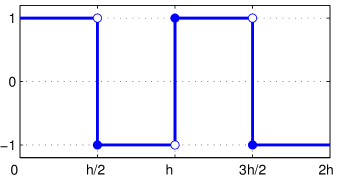
Figure 3.1. Definition of the piecewise constant càdlàg kernel function $\sigma_{h}(x)$.

Assumption 3.1.

In the following, our working assumptions will be that Assumption 2.1 holds for both sub-systems $[\mathbb{N}^{(i)},w^{(i)}(x)]$, $i\in\{1,2\}$ in (3.1)–(3.2) and with the same weight-vector $\boldsymbol{l}$. We separate the constants of the two sub-systems by using superscripts, as in $A^{(i)}$, $i\in\{1,2\}$, and additionally define $A^{(0)}:=A^{(1)}\vee A^{(2)}$.

The assumption that the weight-vector $\boldsymbol{l}$ is the same for both sub-systems as well as for the original description (2.4) is mainly for convenience as it avoids switching back and forth between equivalent norms. A further comment is that, in view of a finite time-step $h$ it makes sense to require that both sub-systems are well-posed in the sense of Theorem 2.1. However, one can rightly ask if this is really necessary as $h\to 0$; for $h$ small enough finite-time explosions are likely not going to be a problem. On balance we chose to settle with the current sufficient conditions as a complete theory likely must contain several special cases (for an illustration, see the numerical example in §4.5).

Theorem 3.1 (Moment bound).

Let $Y(t)$ satisfy (3.6) under Assumption 3.1. Then for any integer $p\geq 1$,

(3.7) $$\operatorname{E}\left\|Y_{t}\right\|_{\boldsymbol{l}}^{p} \leq(\left\|Y_{0}\right\|_{\boldsymbol{l}}^{p}+1)\exp(Ct)-1,$$

with $C>0$ a constant which depends on $p$ and on the relevant constants of the assumptions, but not on the split-step $h$.

It will be convenient to quote the following basic inequality.

Lemma 3.2 (Lemma 4.6 in [15]).

Let $H(x)\equiv(x+y)^{p}-x^{p}$ with $x\in\mathbf{R}_{+}$ and $y\in\mathbf{R}$. Then for integer $p\geq 1$ we have the bounds

(3.8) $$H(x) \leq pyx^{p-1}+2^{p-4}p(p-1)y^{2}\left[x^{p-2}+|y|^{p-2}\right],$$

(3.9) $$|H(x)| \leq p|y|2^{p-2}\left[x^{p-1}+|y|^{p-1}\right].$$

Proof of Theorem 3.1.

The starting point is Dynkin’s formula (2.12) under the stopping time on $\left\|Y_{t}\right\|_{\boldsymbol{l}}$ defined in (2.10). With $f(x)=\left\|x\right\|_{\boldsymbol{l}}^{p}=[\boldsymbol{l}^{T}x]^{p}$ we get

$$\operatorname{E}\left\|Y_{\hat{t}}\right\|_{\boldsymbol{l}}^{p} =\left\|Y_{0}\right\|_{\boldsymbol{l}}^{p}+\operatorname{E}\int_{0}^{\hat{t}}(1+\sigma_{h}(s))\overbrace{\sum_{r\in\mathcal{R}_{1}}w_{r}(Y_{s})\left[\left[\boldsymbol{l}^{T}(Y_{s}-\mathbb{N}_{r})\right]^{p}-\left[\boldsymbol{l}^{T}Y_{s}\right]^{p}\right]}^{=:G_{1}(Y_{s})}\,ds$$

(3.10) $$\hphantom{=\left\|Y_{0}\right\|_{\boldsymbol{l}}^{p}}+\operatorname{E}\int_{0}^{\hat{t}}(1-\sigma_{h}(s))\underbrace{\sum_{r\in\mathcal{R}_{2}}w_{r}(Y_{s})\left[\left[\boldsymbol{l}^{T}(Y_{s}-\mathbb{N}_{r})\right]^{p}-\left[\boldsymbol{l}^{T}Y_{s}\right]^{p}\right]}_{=:G_{2}(Y_{s})}\,ds.$$

Using the assumptions on the first sub-system $[\mathbb{N}^{(1)},w^{(1)}(x)]$ and the first part of Lemma 3.2 we obtain the bound

$$G_{1}(y) \leq p(A^{(1)}+\alpha^{(1)}\left\|y\right\|_{\boldsymbol{l}})\left\|y\right\|_{\boldsymbol{l}}^{p-1}+$$

$$\phantom{\leq}2^{p-3}p(p-1)(B^{(1)}+\beta_{1}^{(1)}\left\|y\right\|_{\boldsymbol{l}}+\beta_{2}^{(1)}\left\|y\right\|_{\boldsymbol{l}}^{2})(\left\|y\right\|_{\boldsymbol{l}}^{p-2}+\delta^{p-2})$$

$$\leq\frac{C}{2}\left(1+\left\|y\right\|_{\boldsymbol{l}}^{p}\right),$$

say, in which $\delta:=\|\boldsymbol{l}^{T}\mathbb{N}^{(1)}\|_{\infty}$ and where Young’s inequality was used several times to arrive at the second bound. A similar bound is readily found for $G_{2}$ so summing up from (3.10) we get

(3.11) $$\operatorname{E}\left\|Y_{\hat{t}}\right\|_{\boldsymbol{l}}^{p} \leq\left\|Y_{0}\right\|_{\boldsymbol{l}}^{p}+\int_{0}^{t}C(1+\operatorname{E}\left\|Y_{\hat{s}}\right\|_{\boldsymbol{l}}^{p})\,ds,$$

where $\hat{s}=s\wedge\tau_{P}$. By Grönwall’s inequality this implies the bound

(3.12) $$\operatorname{E}\left\|Y_{\hat{t}}\right\|_{\boldsymbol{l}}^{p} \leq(\left\|Y_{0}\right\|_{\boldsymbol{l}}^{p}+1)\exp(Ct)-1,$$

which is independent of $P$. We therefore arrive at (3.7) by letting $P\to\infty$ and using Fatou’s lemma. ∎

Recall that the quadratic variation of a process $(X_{t})_{t\geq 0}$ in $\mathbf{R}^{D}$ can be defined by (convergence in probability)

(3.13) $$[X]_{t} =\lim_{\|M\|\to 0}\sum_{k\in M}\left\|X_{t_{k+1}}-X_{t_{k}}\right\|^{2},$$

where the mesh $$M=\{0=t_{0}<t_{1}<\cdots<t_{n}=t\} \|M\|=\max_{k}|t_{k+1}-t_{k}|$$ and where . Similarly, we define for later use also the total variation

(3.14) $$V_{[0,t]}(X) =\lim_{\|M\|\to 0}\sum_{k\in M}\left\|X_{t_{k+1}}-X_{t_{k}}\right\|.$$

Lemma 3.3.

Let $Y(t)$ satisfy (3.6) under Assumption 3.1. Then the quadratic variation of $\left\|Y_{t}\right\|_{\boldsymbol{l}}^{p}$ is bounded by

(3.15) $$\operatorname{E}[\left\|Y\right\|_{\boldsymbol{l}}^{p}]_{t}^{1/2} \leq\operatorname{E}\int_{0}^{t}C(1+\left\|Y_{s}\right\|_{\boldsymbol{l}}^{p}+\beta_{2}^{(0)}\left\|Y_{s}\right\|_{\boldsymbol{l}}^{p+1})\,ds,$$

where $C>0$ again is independent on the split-step $h$ and where $\beta_{2}^{(0)}:=\beta_{2}^{(1)}\vee\beta_{2}^{(2)}$.

Proof.

Instead of as in (3.10), for brevity we shall use the following compact notation for sums involved in the two sub-systems which form the split-step method,

(3.16) $$\sum_{r\in\mathcal{R}_{1},\mathcal{R}_{2}}(1\pm\sigma_{h}(s))F(r) :=\sum_{r\in\mathcal{R}_{1}}(1+\sigma_{h}(s))F(r)+\sum_{r\in\mathcal{R}_{2}}(1-\sigma_{h}(s))F(r).$$

Keeping this in mind we have

(3.17) $$\operatorname{E}\,[\left\|Y\right\|_{\boldsymbol{l}}^{p}]_{\hat{t}}^{1/2} =\operatorname{E}\,\left[\left(\int_{0}^{\hat{t}}\sum_{r\in\mathcal{R}_{1},\mathcal{R}_{2}}\left(\left[\boldsymbol{l}^{T}(Y_{s}-\mathbb{N}_{r})\right]^{p}-\left[\boldsymbol{l}^{T}Y_{s}\right]^{p}\right)^{2}\,\mu_{r}(ds)\right)^{1/2}\right].$$

Writing $\mu_{r}(dt)=(1\pm\sigma_{h}(t))w_{r}(Y_{t-})\,dt+\tilde{\mu}_{r}(dt)$, and from the inequality $\|\cdot\|\leq\|\cdot\|_{1}$ we get after using that the random measure compensated with the deterministic intensity is a local martingale,

(3.18) $$\leq\operatorname{E}\left[\int_{0}^{\hat{t}}\sum_{r\in\mathcal{R}_{1},\mathcal{R}_{2}}(1\pm\sigma_{h}(s))w_{r}(Y_{s})\left|\left[\boldsymbol{l}^{T}(Y_{s}-\mathbb{N}_{r})\right]^{p}-\left[\boldsymbol{l}^{T}Y_{s}\right]^{p}\right|\,ds\right],$$

or, after using Lemma 3.2 (3.9),

$$\leq\operatorname{E}\left[\int_{0}^{\hat{t}}\sum_{r}(1\pm\sigma_{h}(s))\,p|\boldsymbol{l}^{T}\mathbb{N}_{r}|w_{r}(Y_{s})\;2^{p-2}\left[\left\|Y_{s}\right\|_{\boldsymbol{l}}^{p-1}+|\boldsymbol{l}^{T}\mathbb{N}_{r}|^{p-1}\right]\,ds\right]$$

(3.19) $$\leq\operatorname{E}\left[\int_{0}^{\hat{t}}C(B^{(0)}+\beta_{1}^{(0)}\left\|Y_{s}\right\|_{\boldsymbol{l}}+\beta_{2}^{(0)}\left\|Y_{s}\right\|_{\boldsymbol{l}}^{2})\left[\left\|Y_{s}\right\|_{\boldsymbol{l}}^{p-1}+\delta^{p-1}\right]\,ds\right]$$

by Assumption 2.1 (ii), where $\delta=\|\boldsymbol{l}^{T}\mathbb{N}\|_{\infty}$. Using Theorem 3.1 and letting $P\to\infty$ we arrive at the stated bound. ∎

Theorem 3.4.

Let $Y_{t}$ satisfy (3.6) under Assumption 3.1 with $0=\beta_{2}^{(0)}:=\beta_{2}^{(1)}\vee\beta_{2}^{(2)}$. Then if $\left\|Y_{0}\right\|_{\boldsymbol{l}}^{p}<\infty$, $\{Y_{t}\}_{t\geq 0}\in S_{\mathcal{F}}^{p,\mathrm{loc}}(\mathbf{Z}_{+}^{D})$ for all $h>0$. If $\beta_{2}^{(0)}>0$, then the conclusion remains under the additional requirement that $\left\|Y_{0}\right\|_{\boldsymbol{l}}^{p+1}<\infty$.

Note that the somewhat technical details concerning the case $\beta_{2}^{(0)}\not=0$ are shared with the solution of (2.5) itself, see Theorem 2.1.

Proof.

This result follows essentially by combining Theorem 3.1 and Lemma 3.3. We get under the same stopping time as before

$$\left\|Y_{\hat{t}}\right\|_{\boldsymbol{l}}^{p} =\left\|Y_{0}\right\|_{\boldsymbol{l}}^{p}+\int_{0}^{\hat{t}}(1+\sigma_{h}(s))G_{1}(Y_{s})+(1-\sigma_{h}(s))G_{2}(Y_{s})\,ds+M_{\hat{t}},$$

with $G_{1}$ and $G_{2}$ defined in (3.10). The quadratic variation of the local martingale $M_{\hat{t}}$ can be estimated via Lemma 3.3,

(3.20) $$\operatorname{E}\,[M]_{\hat{t}}^{1/2} \leq\operatorname{E}\int_{0}^{\hat{t}}C(1+\left\|Y_{s}\right\|_{\boldsymbol{l}}^{p}+\beta_{2}^{(0)}\left\|Y_{s}\right\|_{\boldsymbol{l}}^{p+1})\,ds.$$

The case $\beta_{2}^{(0)}=0$. Using the bound (3.11) for the drift part as obtained in the proof of Theorem 3.1 we get

$$\left\|Y_{\hat{t}}\right\|_{\boldsymbol{l}}^{p} \leq\left\|Y_{0}\right\|_{\boldsymbol{l}}^{p}+\int_{0}^{\hat{t}}C(1+\left\|Y_{s}\right\|_{\boldsymbol{l}}^{p})\,ds+|M_{\hat{t}}|,$$

combining this with (3.20) we obtain from Burkholder’s inequality [32, Chap. IV.4] that

$$\operatorname{E}\sup_{s\in[0,\hat{t}]}\left\|Y_{s}\right\|_{\boldsymbol{l}}^{p} \leq\left\|Y_{0}\right\|_{\boldsymbol{l}}^{p}+\int_{0}^{\hat{t}}C(1+\operatorname{E}\sup_{s^{\prime}\in[0,s]}\left\|Y_{s^{\prime}}\right\|_{\boldsymbol{l}}^{p})\,ds.$$

It follows that $\operatorname{E}\,\sup_{s\in[0,\hat{t}]}\left\|Y_{s}\right\|_{\boldsymbol{l}}^{p}$ is bounded in terms of the initial data and time $t$. Using Fatou’s lemma the result follows by letting $P\to\infty$.

The case $\beta_{2}^{(0)}>0$. By Theorem 3.1 we still have from (3.20) that

$$\operatorname{E}\,[M]_{\hat{t}}^{1/2} \leq\int_{0}^{\hat{t}}C(1+\operatorname{E}\left\|Y_{s}\right\|_{\boldsymbol{l}}^{p+1})\,ds\leq(e^{C\hat{t}}-1)(\left\|Y_{0}\right\|_{\boldsymbol{l}}^{p+1}+1).$$

where we similarly obtain a bound in terms of the initial data $\|Y_{0}\|^{p+1}$. ∎

3.3. Auxiliary lemmas

It is clear by now that the qualities of the kernel function $\sigma_{h}(\cdot)$ will play a role in the behavior of the split-step method. This motivates the following brief discussion.

Lemma 3.5.

Let $f:\mathbf{R}\to\mathbf{R}$ be a càdlàg piecewise constant function. Then

(3.21) $$\left|\int_{0}^{t}\sigma_{h}(s)f(s)\,ds\right| \leq\frac{h}{2}|f(t)|+\frac{h}{2}V_{[0,t]}(f),$$

where the total absolute variation may be exchanged with the square root of the quadratic variation $[f]_{t}^{1/2}$. Furthermore, if $t$ is a multiple of $h$, then the first term on the right side of (3.21) vanishes.

Proof.

Define

(3.22) $$\Sigma_{h}(t) \equiv\int_{0}^{t}\sigma_{h}(s)\,ds,$$

and observe that $|\Sigma_{h}(\cdot)|\leq h/2$. Denote the left side of (3.21) by $J$. Then with $(t_{k})_{k=0}^{N}$ the points of discontinuity of $f$ in $(0,t)$, but augmented with the two boundary points $\{0,t\}$, we obtain from summation by parts that

$$J =\left|\sum_{k=0}^{N-1}f(t_{k})\;\Delta\Sigma_{h}(t_{k})\right|=\left|f(t)\Sigma_{h}(t)-\sum_{k=0}^{N-1}\Delta f(t_{k})\;\Sigma_{h}(t_{k+1})\right|.$$

The stated result now follows from the triangle inequality and, for the case of the quadratic variation, from the Cauchy-Schwartz inequality. ∎

Lemma 3.6.

Let $G:\mathbf{R}^{D}\to\mathbf{R}$ be a globally Lipschitz continuous function with Lipschitz constant $L$ and let $f:\mathbf{R}\to\mathbf{R}^{D}$ be a piecewise constant càdlàg function. Then

(3.23) $$\left|\int_{0}^{t}\sigma_{h}(s)G(f(s))\,ds\right| \leq\frac{h}{2}|G(f(t))|+\frac{h}{2}LV_{[0,t]}(f),$$

with the same additional variants and simplifications as listed in Lemma 3.5.

Proof.

This follows because $g(t):=G(f(t))$ satisfies the requirements for $f$ in Lemma 3.5; clearly $|\Delta g(t_{k})|=|\Delta G(f(t_{k}))|\leq L\|\Delta f(t_{k})\|$. ∎

3.4. Strong convergence

We are now ready to formulate and prove our main result of the paper.

Theorem 3.7 (Strong convergence).

Let $X(t)$ and $Y(t)$ be solutions to (2.4) and (3.6) with $X_{0}=Y_{0}$ and under Assumptions 2.1 and 3.1, respectively. Then

(3.24) $$\operatorname{E}\|(Y-X)(t)\|^{2} \leq h\,C_{t},$$

for $C_{t}$ some constant dependent on the final time $t$.

In the formulation above, the actual estimate that goes into (3.24) is elaborated upon in (3.28) below. Also, for brevity and inspired by most actual use, we only consider the case of deterministic initial data.

Proof.

Under the stated assumptions both processes are well behaved (Theorem 2.1 and 3.4), so the strategy of proof is to define a suitable stopping time $\tau_{P}$ such that the probability that $t\geq\tau_{P}$ can be made arbitrarily small. We put

$$\tau_{P} :=\inf_{t\geq 0}\{\left\|X_{t}\right\|_{\boldsymbol{l}}\vee\left\|Y_{t}\right\|_{\boldsymbol{l}}>P\},$$

and as before $$\hat{t}=t\wedge\tau_{P}$$. Subtracting (2.4) from (3.6) we get

$$(Y-X)(\hat{t}) =-\sum_{r\in\mathcal{R}_{1},\mathcal{R}_{2}}\mathbb{N}_{r}\Biggl{[}\Pi_{r}\left(\int_{0}^{\hat{t}}(1\pm\sigma_{h}(s))w_{r}(Y_{s-})\,ds\right)-$$

(3.25) $$\hphantom{=-\sum_{r\in\mathcal{R}_{1},\mathcal{R}_{2}}\mathbb{N}_{r}\Biggl{[}}\Pi_{r}\left(\int_{0}^{\hat{t}}w_{r}(X_{s-})\,ds\right)\Biggr{]},$$

where the sign is to be chosen in accordance with (3.16).

Under the stopping time and using the local Lipschitz condition we first produce the basic estimates

$$\int_{0}^{\hat{t}}w_{r}(X_{s-})\,ds\leq\int_{0}^{\hat{t}}w_{r}(0)+PL_{r}\,ds\leq C_{0}^{(r)}(P)\hat{t},$$

$$\int_{0}^{\hat{t}}(1\pm\sigma_{h}(s))w_{r}(Y_{s-})\,ds\leq 2C_{0}^{(r)}(P)\hat{t},$$

with, for brevity, $L_{r}\equiv L_{r}(P)$, and using that $|1\pm\sigma_{h}|=2$.

Taking the square Euclidean norm and expectation value of (3.25) we find by Lemma 2.3 in the form of (2.19) using the above basic bounds that

(3.26) $$\operatorname{E}\|(Y-X)(\hat{t})\|^{2}\leq\|\mathbb{N}\|^{2}\sum_{r=1}^{R}(4C_{0}^{(r)}\hat{t}+1)\operatorname{E}[A_{r}],$$

in terms of

$$A_{r} =\left|\int_{0}^{\hat{t}}w_{r}(Y_{s-})-w_{r}(X_{s-})\,ds\pm\int_{0}^{\hat{t}}\sigma_{h}(s)w_{r}(Y_{s-})\,ds\right|.$$

Using Assumption 2.1 (iii) anew we get

$$A_{r} \leq\int_{0}^{\hat{t}}L_{r}\|(Y-X)(s-)\|\,ds+\underbrace{\left|\int_{0}^{\hat{t}}\sigma_{h}(s)w_{r}(Y_{s-})\,ds\right|}_{=:B_{r}}.$$

Also, by Lemma 3.6 we obtain

$$B_{r} \leq\frac{h}{2}|w_{r}(Y_{\hat{t}-})|+\frac{h}{2}L_{r}[Y]_{\hat{t}-}^{1/2}.$$

For the quadratic variation we note that, since $$\|\cdot\|\leq\|\cdot\|_{1}\leq\left\|\cdot\right\|_{\boldsymbol{l}} [Y]_{t}\leq[\left\|Y\right\|_{\boldsymbol{l}}]_{t} p=1$$, we have that , where the case of Lemma 3.3 applies. Estimating using Theorem 3.1 we get after some work,

(3.27) $$\operatorname{E}[B_{r}] \leq C_{1}^{(r)}(P)h+C_{2}^{(r)}(P)h\hat{t}\,\exp(C\hat{t}),$$

where the constants do not depend on $h$, and where $C_{1}^{(r)}$ may be taken as zero provided that $\hat{t}$ is a multiple of $h$.

Summing this over $r$ we get

$$\operatorname{E}\|(Y-X)(\hat{t})\|^{2} \leq C_{1}h+C_{2}h\hat{t}\,\exp(C\hat{t})+$$

$$\hphantom{\leq}\underbrace{\|\mathbb{N}\|^{2}\sum_{r=1}^{R}(4C_{0}^{(r)}\hat{t}+1)L_{r}}_{=:L(\hat{t})=L(\hat{t},P)}\operatorname{E}\left[\int_{0}^{\hat{t}}\|(Y-X)(s)\|^{2}\,ds\right],$$

where the “integer inequality”, $$n\leq n^{2} n\in\mathbf{Z}$$ for , was used. By Grönwall’s inequality this implies the bound

$$\operatorname{E}\|(Y-X)(\hat{t})\|^{2} \leq h\left[C_{1}+C_{2}\hat{t}\,\exp(C\hat{t})\right]\exp(\hat{t}L(\hat{t})).$$

Using brackets to denote characteristic functions we write

$$\operatorname{E}\|(Y-X)(t)\|^{2} =\operatorname{E}\left[\|(Y-X)(t)\|^{2}[t<\tau_{P}]\right]+\underbrace{\operatorname{E}\left[\|(Y-X)(t)\|^{2}[t\geq\tau_{P}]\right]}_{=:M}.$$

To bound $$M$$, note first that by Cauchy-Schwartz’s inequality,

$$M \leq\left(\operatorname{E}\|(Y-X)(t)\|^{4}\right)^{1/2}\left(\mathbf{P}[t\geq\tau_{P}]\right)^{1/2}.$$

Since $$\mathbf{P}[t\geq\tau_{P}]=\mathbf{P}[\sup_{s\in[0,t]}\left\|X_{s}\right\|_{\boldsymbol{l}}\vee\left\|Y_{s}\right\|_{\boldsymbol{l}}>P]$$ we get from Markov’s inequality

$$M \leq\left(\operatorname{E}\|(Y-X)(t)\|^{4}\right)^{1/2}P^{-1/2}\left(\operatorname{E}\sup_{s\in[0,t]}\left\|X_{s}\right\|_{\boldsymbol{l}}\vee\left\|Y_{s}\right\|_{\boldsymbol{l}}\right)^{1/2}.$$

By Theorem 2.1 and 3.4 we find that $M$ converges to zero as $P\to\infty$. In particular, for any given $\varepsilon\in(0,1)$, we can find $P$ large enough (and hence also $C_{1}$, $C_{2}$, and $L(t)$) such that

$$M \leq\varepsilon\operatorname{E}\|(Y-X)(t)\|^{2}.$$

Combining we thus get

(3.28) $$\operatorname{E}\|(Y-X)(t)\|^{2} \leq\frac{h}{1-\varepsilon}\left[C_{1}+C_{2}t\,\exp(Ct)\right]\exp(tL(t)),$$

where $C_{1}$, $C_{2}$, and $L(t)$ depend on $\varepsilon$ via the choice of $P$. ∎

We now offer some brief comments on this result. The estimated error growth in any given interval of time $[0,t]$ is clearly quite pessimistic, but is on the other hand also quite general, relying as it does mainly on the existence of local Lipschitz constants. Also, the fact that the constant $C_{1}$ may be disregarded when $t$ is a multiple of the split-step $h$, is perhaps mostly of theoretical interest as the other terms seem to dominate by far. One may simply think of this as a smaller error when the split-step solution is viewed at the discrete mesh $[0,h,2h,\ldots]$.

Finally we comment also that Theorem 3.7 may be strengthen in the direction of convergence in

(3.29) $$\operatorname{E}\sup_{s\in[0,t]}\|(Y-X)(t)\|^{2},$$

by bounding the martingale part and relying on Burkholder’s inequality. Since this is somewhat tedious and does not add much insight we have chosen to omit it altogether.

4. Numerical examples

To illustrate the theory developed in the previous sections, but also as a means to investigate the sharpness of some of the bounds, a few selected numerical examples are presented here. In §4.1 we briefly discuss the actual implementation of the method implied by (3.6), and in §4.2 and §4.3 the convergence of the split-step method applied to two one-dimensional examples is investigated. Concretely, our computational analysis investigates the convergence dependency in the presence of non-linearities, the weak convergence behavior, and the qualities of higher order split-step methods. In §4.4 convergence over longer time-intervals is discussed and in §4.5, finally, we look at a split which violates Assumption 3.1.

4.1. Implementation

The idea to use the operational time representation (2.4) to devise computational algorithms has been employed previously for time-parallel algorithms [17] and for parameter sensitivity computations [7, 35]. The Common Reaction Path Method [35] simulates (2.4) using $R$ separate streams of random numbers and can be regarded as a careful implementation of the Next Reaction Method [20] such that a consistent operational time is always defined. An additional improvement reported for spatial problems in [7] is to handle rates that become zero in a somewhat careful way. By explicitly storing the operational time $\tau^{\mathrm{old}}$ and associated rate $w^{\mathrm{old}}$ before the rate vanished we can “activate” the reaction channel by using the rescaling technique [20],

(4.1) $$\tau^{\mathrm{new}}=t_{\mathrm{current}}+\left(\tau^{\mathrm{old}}-t_{\mathrm{current}}\right)w^{\mathrm{old}}/w^{\mathrm{new}},$$

where $w^{\mathrm{new}}$ is the first non-zero rate encountered. As opposed to drawing a new random number whenever the channel is reactivated, this technique preserves the consistency of the current operational time.

All these implementation techniques transfer nicely to the split-step formulation (3.6). The kernel function $\sigma_{h}$ may be thought of as generating deterministic events at points in time which are multiples of $h/2$, where the active and passive pathways simply change roles. Besides being able to compare trajectories path-wise for different values of $h$, a great feature with this implementation strategy is of course that the limit $h\to 0$ is directly computable.

For the computations presented below we used the estimator

(4.2) $$\operatorname{E}[(Y-X)(t)]^{2} \approx M\equiv\frac{1}{N}\sum_{i=1}^{N}(Y-X)(t;\omega_{i})^{2},$$

where $$\omega_{i}$$ indicate independent trajectories coupled and computed according to the previous description. To estimate the uncertainty in (4.2) we compute

(4.3) $$S^{2} \equiv\frac{1}{N-1}\sum_{i=1}^{N}\left[(Y-X)(t;\omega_{i})^{2}-M\right]^{2},$$

and use a suitable multiple of $S/\sqrt{N}$ as a measure of the uncertainty.

4.2. Linear birth-death process

We first consider the model

(4.4) $$\emptyset\xrightleftharpoons[\mu X]{k}X,$$

with $[k,\mu]=[5,0.05]$ for time $t\in[0,100]$ and with $X(0)=50$. This model approaches a steady-state Poissonian distribution around the mean value 100 and executes about $10^{3}$ events in the given time interval. Sample illustrations of this process are displayed in Figure 4.1.

In the notation of Assumption 2.1 the birth-death model is characterized by $\alpha=-\mu$, $\beta_{1}=\mu/2$, and $\beta_{2}=0$. By the negative sign of $\alpha$, the dynamics is dissipative for states $x>k/\mu$ and we note also that the propensities are globally Lipschitz with constant $L=\mu$. Computational results are reported in comparison with the dimerization model, next to be introduced.

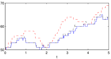
Figure 4.1. Sample trajectories of the linear birth-death model. Solid: direct simulation, dashed: split-step solution ($h=2$), dash-dot: split-step solution ($h=1/4$). For $h=2$ the periodic effect of the kernel function $\sigma_{h}$ is clearly visible.

4.3. Dimerization

As a simple nonlinear extension of (4.4) we consider

(4.5) $$\emptyset\xrightarrow{k}X,\quad X+X\xrightarrow{\nu X(X-1)}\emptyset.$$

We normalize the model such that the equilibrium mean $\sqrt{k/(2\nu)}$ coincide with that of (4.4) and we also use the same birth constant $k$. This means that for both models, about the same number of events is generated in the considered interval of time.

It is instructive to try to reason about the effect of the non-linearity in (4.5) in comparison with the fully linear model (4.4). Although by necessity $\alpha=0$ in Assumption 2.1 (i), it still holds true that the dynamics is dissipative for states larger than the equilibrium mean value. Also, due to the quadratic reaction, there is no longer a global Lipschitz constant in Assumption 2.1 (iii), but one may note that close to the equilibrium mean value, $L\sim\nu\times(x-1)\sim\mu^{2}/(2k)\times k/\mu=\mu/2$. Since the quadratic reaction involves two molecules one may argue that the effective Lipschitz constant for (4.5) approximately matches that of (4.4).

A more striking difference between the two models can be found in Assumption 2.1 (ii). Namely, for (4.5) the left side reads

(4.6) $$k/2\left[1+4\nu/k\times x(x-1)\right] \sim 3k/2,$$

whereas for (4.4) we have

(4.7) $$k/2\left[1+\mu/k\times x\right] \sim k,$$

again, assuming that $x$ is close to the equilibrium mean value.

4.3.1. Strong convergence

We first consider the strong convergence of the split-step method. The mean square error as a function of the split-step $h$ is shown in Figure 4.2 and the results show that, although both the birth-death model (4.4) and the dimerization model (4.5) are unbounded problems, the strong order is still $1/2$ as predicted by Theorem 3.7.

The interesting observation to be made is that, with the exception of the case $h=1$, the mean square error for the dimerization problem is consistently almost a factor of two larger than for the birth-death problem (the measured factor falls in the range $[1.5,2.1]$ for the cases studied). It is not easy to strictly analyze the reasons behind this phenomenon but we may argue heuristically as follows.

Let us take (3.28) in Theorem 3.7 for some fixed value of $\varepsilon$ as an estimate of the error. By the set-up of the measurements, $C_{1}=0$ in (3.28), and we have also argued previously that the effective Lipschitz constants for the two models are about the same. The difference between the two models has therefore been isolated to the expression $C_{2}ht\exp(Ct)$ in the right side of (3.28), which can be traced back to the bound of $B_{r}$ in (3.27). In turn, this estimate comes from the bound on the quadratic variation in Lemma 3.3 and relies indirectly also on the moment estimate from Theorem 3.1. In the present case the first few moments of (4.4) and (4.5) are of comparable magnitude so we thus focus our attention to the constant $C$ in (3.15) of Lemma 3.3. In the proof, this constant emerges in (3.19) and is a direct consequence of Assumption 2.1 (ii).

This assumption was investigated in (4.6)–(4.7) above where we found a difference between the two models in the form of an overall factor of $3/2$ and a factor of $2$ when considering the non-constant part, in striking agreement with the measured factor $\in[1.5,2.1]$.

It is an interesting and challenging question if the above heuristic way of reasoning can somehow be put on firm grounds. In particular, it would be very useful if the use of ‘effective’ Lipschitz constants could render a consistent analysis.

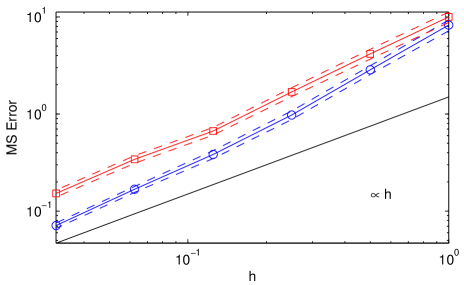
Figure 4.2. Convergence in mean square of the split-step method with decreasing $h$ for the linear birth-death model (4.4) (circles) and for the dimerization (4.5) (squares). Dashed lines indicate the estimator’s uncertainty $\pm S/\sqrt{N}$ (cf. (4.3)). For both cases the method converges faster initially but approaches the strong order $1/2$ as $h$ becomes smaller.

4.3.2. Weak convergence

We briefly look also at the weak convergence of the split-step scheme. Hence we estimate for varying split-step $h$,

(4.8) $$\left|\operatorname{E}[f(Y_{t})]-\operatorname{E}[f(X_{t})]\right|,$$

with $$f$$ some smooth function and otherwise following the computational procedure in §4.1. To be concrete we took

(4.9) $$f_{1}(x)=x,$$

(4.10) $$f_{2}(x)=x(x-1),$$

that is, the first two factorial moments. In analogy with Figure 4.2, in Figure 4.3 we report the error (4.8) for these two cases. As expected we find a first order weak error when measured in the split-step $h$. Perhaps more interesting is the observation that the errors for the two models are very similar and that there is no visible impact from the non-linearity.

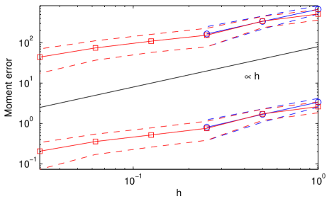
Figure 4.3. Weak convergence of the split-step method with decreasing $h$. Circles: linear birth-death model (4.4) and squares: dimerization (4.5). Top: second order factorial moment, bottom: first order factorial moment. For the birth-death model, only data for the larger values of $h$ are available as the variance was too large to determine the sign of the error within the target uncertainty.

4.3.3. The 2nd order Strang split

The second order Strang split is traditionally written in operator form in the style of (3.3)–(3.4),

(4.11) $$\tilde{p}_{h}(x,t+h/2) =p_{h}(x,t)+\int_{t}^{t+h/2}\sum_{r\in\mathcal{R}_{1}}w_{r}(x+\mathbb{N}_{r})\tilde{p}_{h}(x+\mathbb{N}_{r},s)-w_{r}(x)\tilde{p}_{h}(x,s)\,ds,$$

(4.12) $$\tilde{\tilde{p}}_{h}(x,t+h) =\tilde{p}_{h}(x,t+h/2)+\int_{t}^{t+h}\sum_{r\in\mathcal{R}_{2}}w_{r}(x+\mathbb{N}_{r})\tilde{\tilde{p}}_{h}(x+\mathbb{N}_{r},s)-w_{r}(x)\tilde{\tilde{p}}_{h}(x,s)\,ds,$$

(4.13) $$p_{h}(x,t+h) =\tilde{\tilde{p}}_{h}(x,t+h)+\int_{t+h/2}^{t+h}\sum_{r\in\mathcal{R}_{1}}w_{r}(x+\mathbb{N}_{r})p_{h}(x+\mathbb{N}_{r},s)-w_{r}(x)p_{h}(x,s)\,ds,$$

which via two intermediate steps takes us from time $t$ to $t+h$. A moments consideration gives that this is just the same thing as substituting the kernel function $\sigma_{h}(s)$ in (3.6) with the time shifted version $\sigma_{h}(s+h/4)$. Importantly, the resulting compact notation is open to the same kind of analysis performed in §3 and we draw the conclusion that also this method can be expected to converge at strong order $1/2$. We should mention though, that to strictly prove that the convergence order is not actually higher might require some more work.

A feature with the split method (4.11)–(4.13) is that it can be expected to be second order weakly convergent. This follows heuristically from the fact that it is a second order operator splitting method in the finite-dimensional case, and hence can be expected to perform as such also in cases that are of effectively bounded character.

In Figure 4.4 we display the mean square strong error as a function of the split-step $h$ for the two models considered in this section. The asymptotic behavior is quite similar to Figure 4.2 in that we still approach the strong order $1/2$ as $h\to 0$ and in that the error reduction factor between the two models is about the same, or perhaps slightly larger $\in[1.7,3.2]$.

By far the most striking difference is that the mean square error is now between 1.5 to 2 orders smaller than before. It is unfortunately quite difficult to explain this in the setting of §3.4 since the analysis there would be quite similar upon substituting $\sigma_{h}(s)\mapsto\sigma_{h}(s+h/4)$. In particular, assuming the Strang split to be second order weakly convergent, it is difficult to see where this feature could enter the analysis effectively.

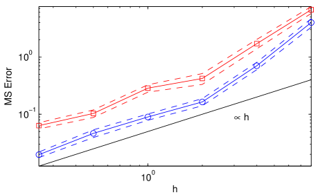
Figure 4.4. Convergence in mean square of the Strang split method (4.11)–(4.13), following closely the notation in Figure 4.2. Although the asymptotic strong order of convergence is still $1/2$, the error is considerably smaller for the same values of $h$.

4.4. Elementary bimolecular reaction, case of no equilibrium

As a slightly more involved model we consider the following bimolecular birth-death system,

(4.17) $$\left.\begin{array}[]{c}\emptyset\xrightarrow{k_{1}}X\\ \emptyset\xrightarrow{k_{1}}Y\\ X+Y\xrightarrow{k_{2}XY}\emptyset\end{array}\right\},$$

with the stoichiometric matrix

(4.18) $$\mathbb{N} =\begin{bmatrix}[r]-1&0&1\\ 0&-1&1\end{bmatrix}$$

and reaction propensities $w(x)=[k_{1},k_{1},k_{2}x_{1}x_{2}]^{T}$ for $x=[x_{1},x_{2}]^{T}$.

To get some feeling for the behavior of (4.17), we define the difference process $U(t)=(X-Y)(t)\in\mathbf{Z}$. From Itô’s formula (2.11) with $f(x)=x_{1}-x_{2}$ we get

(4.19) $$dU_{t} =df(X_{t})=-[-1,1,0]\,\boldsymbol{\mu}(dt),$$

which is equivalent to the model

(4.20) $$\emptyset\xrightleftharpoons[k_{1}]{k_{1}}U,$$

which is just a constant intensity random walk on all of $\mathbf{Z}$. One can solve this explicitly in terms of two independent Poisson distributions,

(4.21) $$U_{t} =U_{0}+\Pi_{1}(k_{1}t)-\Pi_{2}(k_{1}t)\sim U_{0}+\mathcal{N}(U_{0},2k_{1}t),\quad\mbox{$t\to\infty$,}$$

for $\mathcal{N}$ a Gaussian random variable of the indicated mean and variance. Hence the system takes longer and longer excursions away from the origin and we have an example of an equilibrium density which clearly does not exist.

We split the problem (4.17) with $\mathcal{R}_{1}=\{1,2\}$ and $\mathcal{R}_{2}=\{3\}$, that is, with the two birth processes evolved simultaneously. In Figure 4.5 we display the mean square error as a function of time for several values of the split-step parameter $h$. Experimentally we find that the strong order of convergence is still $1/2$ even for quite long simulation times and despite the fact that the behavior of the underlying process is open, visiting states further and further away.

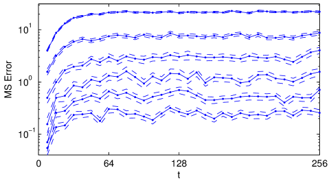
Figure 4.5. Mean square error of the split-step method for the bimolecular problem (4.17) as a function of time $t$. From top to bottom: $h=[4,2,1,1/2,1/4,1/8]$. The asymptotic strong order of the method is $q\approx[0.76,0.67,0.67,0.61,0.55]$ for the cases shown in the figure and averaging over the data for $t\in[128,256]$.

4.5. An ill-posed split

In this section we apply the split-step method to a model which does not comply with Assumption 3.1. This is quite challenging computationally and thus the model settled for was selected after trying several quite different cases. Although somewhat artificially looking, the rather simple system chosen was

(4.24) $$\left.\begin{array}[]{ll}\emptyset\xrightarrow{10}X&3X\xrightarrow{x(x-1)(x-2)/2}X\\ 3X\xrightarrow{x(x-1)(x-2)/2}X&3X\xrightarrow{x(x-1)(x-2)}4X\end{array}\right\}.$$

The stoichiometric vector is given by $\mathbb{N}=[-1,-2,-2,1]$ and hence the problem is very strongly dissipative for states large enough in view of the fact that the ingoing cubic reactions dominates. However, by splitting the system according to $\mathcal{R}_{1}=\{1,2\}$ and $\mathcal{R}_{2}=\{3,4\}$, we have that the second pair violates Assumption 3.1. In fact, this sub-system can be shown to explode in the second moment for $t\lesssim X(0)^{-3}/3$ whenever $X(0)\geq 3$ despite the fact that the net drift is zero [15, Proposition 4.1].

In the simulation we worked with the stopped process $\hat{X}(t)=X(t)\wedge P$, where $P=10^{3}$ was used and where $t\in[0,1]$ with $X(0)=10$ was considered. In Figure 4.6 we report the results of a convergence study for a selection of comparably small split-step sizes $h$. The convergence behavior is rather intriguing, with an initial much slower strong order convergence rate of about $1/4$, but which picks up speed for $h$ smaller than about $10^{-3}/3$, which is also approximately the maximum time interval over which the second sub-system does not explode in variance. Although the method still seems to converge, the effects of choosing a split containing an ill-posed sub-system are clearly visible.

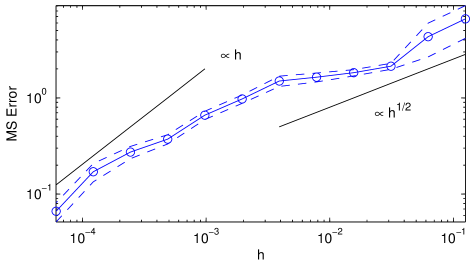
Figure 4.6. Mean square convergence for the split-step method applied to the problem (4.24), for which one of the sub-systems is ill-posed in the sense of unbounded second moments in finite time. The order of convergence is roughly $1/4$ for the range of $h$ studied here but appears to improve somewhat towards the smaller values.

5. Conclusions

We have proposed a framework for analyzing certain popular split-step methods for jump stochastic differential equations. The framework consists of a formulation of the methods in operational time via the split-step kernel function, enabling a meaningful path-wise coupling even in the limit $h\to 0$. We have also presented concrete assumptions and a priori results which together with the theoretical convergence results form a basis for the sound use and further development of these types of methods.

In performing the computational experiments we also developed an actual implementation of our formulation which is useful in assessing the split-step solution quality as a function of various parameters. For example, this is important when experimentally approaching set-ups for which the proposed sufficient conditions for convergence are violated.

The numerical experiments illustrate the theory in different ways and also open up some intriguing questions. For instance, how can the surprisingly good relative efficiency of the second order Strang method versus the simpler first order method best be explained in the setting of strong convergence? We also observed a better convergence over longer time intervals than perhaps intuitively expected, and we noted that the method converges even in a case for which one of the split sub-systems was ill-posed in the sense of finite-time moment explosions.

More practically, an important and natural extension is when the different sub-systems are evolved by specially designed approximative methods, a quite common approach in multiscale and multiphysics problems. The proposed framework should remain a viable approach as long as these methods may also be analyzed in a path-wise sense, a point to which we intend to return to in future work.

References

- Anderson [2008] D. F. Anderson. Incorporating postleap checks in tau-leaping. J. Chem. Phys., 128(5):054103–054111, 2008. doi:10.1063/1.2819665.
- Anderson et al. [2011] D. F. Anderson, A. Ganguly, and T. G. Kurtz. Error analysis of tau-leap simulation methods. Ann. Appl. Probab., 21(6):2226–2262, 2011. doi:10.1214/10-AAP756.
- Applebaum [2004] D. Applebaum. Lévy Processes and Stochastic Calculus, volume 93 of Cambridge Studies in Advanced Mathematics. Cambridge University Press, Cambridge, 2004.
- Arampatzis et al. [2014] G. Arampatzis, M. Katsoulakis, and P. Plecháč. Parallelization, processor communication and error analysis in lattice kinetic monte carlo. SIAM J. Numer. Anal., 52(3):1156–1182, 2014. doi:10.1137/120889459.
- Ball et al. [2006] K. Ball, T. G. Kurtz, L. Popovic, and G. Rempala. Asymptotic analysis of multiscale approximations to reaction networks. Ann. Appl. Probab., 16(4):1925–1961, 2006. doi:10.1214/105051606000000420.
- Barkai and Leibler [2000] N. Barkai and S. Leibler. Circadian clocks limited by noise. Nature, 403:267–268, 2000. doi:10.1038/35002258.
- Bauer and Engblom [2015] P. Bauer and S. Engblom. Sensitivity estimation and inverse problems in spatial stochastic models of chemical kinetics. In A. Abdulle, S. Deparis, D. Kressner, F. Nobile, and M. Picasso, editors, Numerical Mathematics and Advanced Applications: ENUMATH 2013, volume 103 of Lecture Notes in Computational Science and Engineering, pages 519–527, Berlin, 2015. Springer. doi:10.1007/978-3-319-10705-9_51.
- Bayati [2013] B. S. Bayati. Fractional diffusion-reaction stochastic simulations. J. Chem. Phys., 138(10):104117, 2013. doi:10.1063/1.4794696.
- Brémaud [1981] P. Brémaud. Point Processes and Queues: Martingale Dynamics. Springer Series in Statistics. Springer, New York, 1981.
- Brémaud [1999] P. Brémaud. Markov Chains: Gibbs Fields, Monte Carlo Simulation, and Queues. Number 31 in Texts in Applied Mathematics. Springer, New York, 1999.
- Briat et al. [2014] C. Briat, A. Gupta, and M. Khammash. A scalable computational framework for establishing long-term behavior of stochastic reaction networks. PLoS Comput. Biol., 10(6):e1003669, 2014. doi:10.1371/journal.pcbi.1003669.
- Cao et al. [2005] Y. Cao, D. Gillespie, and L. Petzold. Multiscale stochastic simulation algorithm with stochastic partial equilibrium assumption for chemically reacting systems. J. Comput. Phys., 206:395–411, 2005. doi:10.1016/j.jcp.2004.12.014.
- Chevallier and Engblom [2015] A. Chevallier and S. Engblom. Pathwise error bounds in multiscale variable splitting methods for spatial stochastic kinetics, 2015. Manuscript.
- E et al. [2005] W. E, D. Liu, and E. Vanden-Eijnden. Nested stochastic simulation algorithm for chemical kinetic systems with disparate rates. J. Chem. Phys., 123(19):194107, 2005. doi:10.1063/1.2109987.
- Engblom [2014] S. Engblom. On the stability of stochastic jump kinetics. Appl. Math., 5(19):3217–3239, 2014. doi:10.4236/am.2014.519300.
- S. Engblom and L. Ferm and A. Hellander and P. Lötstedt [2009] S. Engblom and L. Ferm and A. Hellander and P. Lötstedt. Simulation of stochastic reaction-diffusion processes on unstructured meshes. SIAM J. Sci. Comput., 31(3):1774–1797, 2009. doi:10.1137/080721388.
- S. Engblom [2009] S. Engblom. Parallel in time simulation of multiscale stochastic chemical kinetics. Multiscale Model. Simul., 8(1):46–68, 2009. doi:10.1137/080733723.
- Ethier and Kurtz [1986] S. N. Ethier and T. G. Kurtz. Markov Processes: Characterization and Convergence. Wiley series in Probability and Mathematical Statistics. John Wiley & Sons, New York, 1986.
- Ganguly et al. [2014] A. Ganguly, D. Altıntan, and H. Koeppl. Jump-diffusion approximation of stochastic reaction dynamics: Error bounds and algorithms, 2014. Available at http://arxiv.org/abs/1409.4303.
- Gibson and Bruck [2000] M. A. Gibson and J. Bruck. Efficient exact stochastic simulation of chemical systems with many species and many channels. J. Phys. Chem., 104(9):1876–1889, 2000. doi:10.1021/jp993732q.
- Gillespie [1976] D. T. Gillespie. A general method for numerically simulating the stochastic time evolution of coupled chemical reactions. J. Comput. Phys., 22(4):403–434, 1976. doi:10.1016/0021-9991(76)90041-3.
- Gillespie [1992] D. T. Gillespie. A rigorous derivation of the chemical master equation. Phys. A, 188:404–425, 1992. doi:10.1016/0378-4371(92)90283-V.
- Gillespie [2001] D. T. Gillespie. Approximate accelerated stochastic simulation of chemically reacting systems. J. Chem. Phys., 115(4):1716–1733, 2001. doi:10.1063/1.1378322.
- Goutsias [2005] J. Goutsias. Quasiequilibrium approximation of fast reaction kinetics in stochastic biochemical systems. J. Chem. Phys., 122(18):184102, 2005. doi:10.1063/1.1889434.
- Haseltine and Rawlings [2002] E. L. Haseltine and J. B. Rawlings. Approximate simulation of coupled fast and slow reactions for stochastic chemical kinetics. J. Chem. Phys., 117(15):6959–6969, 2002. doi:10.1063/1.1505860.
- Hellander et al. [2014] A. Hellander, M. J. Lawson, B. Drawert, and L. Petzold. Local error estimates for adaptive simulation of the reaction-diffusion master equation via operator splitting. J. Comput. Phys., 266(0):89–100, 2014. doi:10.1016/j.jcp.2014.02.004.
- Jahnke and Altıntan [2010] T. Jahnke and D. Altıntan. Efficient simulation of discrete stochastic reaction systems with a splitting method. BIT, 50(4):797–822, 2010. doi:10.1007/s10543-010-0286-0.
- N. G. van Kampen [2004] N. G. van Kampen. Stochastic Processes in Physics and Chemistry. Elsevier, Amsterdam, 2nd edition, 2004.
- Kurtz [1978] T. G. Kurtz. Strong approximation theorems for density dependent Markov chains. Stochastic Process. Appl., 6(3):223–240, 1978. doi:10.1016/0304-4149(78)90020-0.
- Li [2007] T. Li. Analysis of explicit tau-leaping schemes for simulating chemically reacting systems. Multiscale Model. Simul., 6(2):417–436, 2007. doi:10.1137/06066792X.
- Paulsson et al. [2000] J. Paulsson, O. G. Berg, and M. Ehrenberg. Stochastic focusing: Fluctuation-enhanced sensitivity of intracellular regulation. Proc. Natl. Acad. Sci. USA, 97(13):7148–7153, 2000. doi:10.1073/pnas.110057697.
- Protter [2005] P. E. Protter. Stochastic Integration and Differential Equations. Number 21 in Stochastic Modelling and Applied Probability. Springer, Berlin, 2nd edition, 2005. Version 2.1.
- Rathinam [2015] M. Rathinam. Moment growth bounds on continuous time Markov processes on non-negative integer lattices. Quart. Appl. Math., 73(2):347–364, 2015. doi:10.1090/S0033-569X-2015-01372-7.
- Rathinam et al. [2005] M. Rathinam, L. R. Petzold, Y. Cao, and D. T. Gillespie. Consistency and stability of tau-leaping schemes for chemical reaction systems. Multiscale Model. Simul., 4(3):867–895, 2005. doi:10.1137/040603206.
- Rathinam et al. [2010] M. Rathinam, P. W. Sheppard, and M. Khammash. Efficient computation of parameter sensitivities of discrete stochastic chemical reaction networks. J. Chem. Phys., 132(3):034103, 2010. doi:10.1063/1.3280166.
- Situ [2005] R. Situ. Theory of Stochastic Differential Equations with Jumps and Applications. Mathematical and Analytical Techniques with Applications to Engineering. Springer, New York, 2005.
- Strang [1968] G. Strang. On the construction and comparison of difference schemes. SIAM J. Numer. Anal., 5(3):506–517, 1968. doi:10.1137/0705041.
- Togashi and Kaneko [2004] Y. Togashi and K. Kaneko. Molecular discreteness in reaction-diffusion systems yields steady states not seen in the continuum limit. Phys. Rev. E, 70(2):020901–1, 2004. doi:10.1103/PhysRevE.70.020901.