Using Python to Dive into Signalling Data with CellNOpt and BioServices

Abstract

Systems biology is an inter-disciplinary field that studies systems of biological components at different scales, which may be molecules, cells or entire organism. In particular, systems biology methods are applied to understand functional deregulations within human cells (e.g., cancers). In this context, we present several python packages linked to CellNOptR (R package), which is used to build predictive logic models of signalling networks by training networks (derived from literature) to signalling (phospho-proteomic) data. The first package (cellnopt.wrapper) is a wrapper based on RPY2 that allows a full access to CellNOptR functionalities within Python. The second one (cellnopt.core) was designed to ease the manipulation and visualisation of data structures used in CellNOptR, which was achieved by using Pandas, NetworkX and matplotlib. Systems biology also makes extensive use of web resources and services. We will give an overview and status of BioServices, which allows one to access programmatically to web resources used in life science and how it can be combined with CellNOptR.

1 Context and Introduction

Systems biology studies systems of biological components at different scales, which may be molecules, cells or entire organisms. It is a recent term that emerged in the 2000s [IDE01], [KIT02] to describe an inter-disciplinary research field in biology. In human cells, which will be considered in this paper, systems biology helps to understand functional deregulations inside the cells that are induced either by gene mutations (in the nucleus) or extracellular signalling. Such deregulations may lead to the apparition of cancers or other diseases.

Cells are constantly stimulated by extracellular signalling. Receptors on the cell surface may be activated by those signals thereby triggering a chain of events inside the cell (signal transduction). These chains of events are also called signalling pathways. Depending on the response, the cell behaviour may be altered (shape, gene expression, etc.). These pathways are connected to dense network of interactions between proteins that propagate the external signals down to the gene expression level (see Figure 1). For simplicity, relationships between proteins are often considered to be either activation or inhibition. In addition, protein complexes may also be formed, which means that several type of proteins may be required to activate or inhibit another protein. Protein interaction networks are complex:

• the number of protein types is large (about 20,000 in human cells)

• signalling pathways are context specific and cell-type specific; there are about 200 human cell types (e.g., blood, liver)

• proteins may have different dynamic (from a few minutes to several hours).

A classical pathway example is the so-called P53 pathway (see Figure 1). In a normal cell the P53 protein is inactive (inhibited by the MDM2 protein). However, upon DNA damage or other stresses, various pathways will lead to the dissociation of this P53-MDM2 complex, thereby activating P53. Consequently, P53 will either prevent further cell growth to allow a DNA repair or initiate an apoptosis (cell death) to discard the damaged cell. A deregulation of the P53 pathway would results in an uncontrolled cell proliferation, such as cancer [HAUPT].

Figure 1: Overview of signal transduction pathways. The cell boundary (thick orange line) has receptors to external signals (e.g., survival factors IGF1). These signals propagate inside the cell via complex networks of protein interactions (e.g., activation and inhibition) down to the gene expression level inside the cell nucleus (red thick line). Image source: wikipedia.

In order to predict novel therapeutic solutions, it is essential to understand the behaviour of signalling pathways. Discrete logic modelling provides a framework to link signalling pathways to extracellular signals and drug effects [SAEZ]. Experimental data can be obtained by measuring protein responses to combination of drugs (altering normal behaviour of a protein) and stimulations. There are different type of experiments from mass-spectrometry (many proteins but few perturbations) to antibody-based experiments (few proteins but more time points and perturbations).

The software CellNOptR [CNO12] provides tools to perform logic modeling at the protein level using network of protein interactions and perturbation data sets. The core of the software consist in (1) transforming a protein network into a logical network; (2) simulating the flow of signalling in the network using for instance a boolean formalism; (3) comparing real biological data with the simulated data. The software is essentially an optimisation problem, which can be solved by various algorithms (e.g., genetic algorithm).

Although CellNOpt is originally written with the R language, we will focus on two python packages that are related to it. The first one called cellnopt.wrapper is a Python wrapper that have been written using the RPy2 package. The second package is called cellnopt.core. It combines several libraries (e.g., Pandas [MCK10], NetworkX [ARI08] and Matplotlib [HUN07]) to provide tools dedicated to the manipulation of network of proteins and perturbation data sets that are the input of CellNOptR packages.

Another important need of systems biology is to be able to access online resources and databases. In the context of logical modeling, resources of importance are signalling pathways (e.g., Wiki Pathway [WP09]) and retrieval of information about proteins (e.g., UniProt [UNI14]). In order to help us in this task, we developed BioServices [COK13] that ease programmatic access to web services in Python. It was then extended to retrieve information from other web services so as to cover the spectrum of bioinformatics resources (e.g., genomics, sequence analysis).

In the first part of this paper, we will briefly present the data structure used in CellNOptR and a typical pipeline. We will then demonstrate how cellnopt.wrapper and cellnopt.core can enhance user experience. In the second part, we will quickly present BioServices and give an update on its status and future directions.

2 CellNOpt

CellNOptR [CNO12] is a R package used for creating logic-based models of signal transduction networks using different logic formalisms but we consider boolean logic only here below. Other formalisms including differential equation formalism are covered in [MAC12] , [CNO12].

In a nutshell, CellNOptR uses information on signalling pathways encoded as a Prior Knowledge Network (PKN), and trains it against high-throughput biochemical data to create cell-specific models. The training is performed with optimisation such as genetic algorithms. For more details see also the www.cellnopt.org website.

2.1 Input data structures

2.1.1 Network and logic model

Figure 2: Prior Knowledge Network (PKN) example. Colored nodes represent (i) stimuli (green, generally on cell surface or close to), (ii) measured proteins (blue), (iii) inhibited protein by a drug (red), (iv) silent nodes (white and grey) that do not affect the logic of the model if removed. Black edges represent activation and red edges represent inhibition.

The PKNs gives a list of known relationships between proteins. It is built from literature or expertise from experimentalists. One way to store the PKNs is to use the SIF format, which list relationships between proteins within a tabulated-separated values file. Consider this example:

Input1 1 Interm
Input2 1 Interm
Interm 1 Output

Each row is a reaction where the first element is the input protein, the third element is the affected protein, and the middle element is the relationship, where 1 means activation and -1 means inhibition. A visual representation of this example is shown in Figure 5. A more realistic example is also provided in Figure 2. Such networks are directed graphs where edges can be either activation (represented by normal black edge) or inhibition (represented by the red edge).

In the SIF file provided above, only OR relationships are encoded: the protein Interm is activated by the Input1 OR Input2 protein. Within cells, complex of proteins do exist, which means that an AND relationship is also possible. Transforming the input PKN into a logical model means that AND gates have to be added (if there are several inputs).

2.1.2 Data

The data used in CellNOpt is made of measurements of protein responses to perturbations, which is a combination of stimuli (on cell receptor) and inhibition (caused by a drug treatment). These measurements are stored in a format called MIDAS [MIDAS], which is a CSV file format. Figure 3 gives an example of a MIDAS data file together with further explanations.

2.1.3 Training

Once a PKN and a MIDAS file are in place, the PKN is transformed into a logic model. Further simplifications can be applied on the model as shown in Figure 5 (e.g., compression to remove nodes/proteins that do not change the logic of the network). Finally, the training of the logic model to the data is performed by minimising an objective function written as follows:

$$\theta(M)=\theta_{f}(M)+\alpha\theta_{s}(M)$$

where

$$\theta_{f}(M)=\frac{1}{N}\sum_{k=1}^{K}\sum_{e=1}^{E}\sum_{t=1}^{T}(X_{k,e,t}-X_{k,e,t}^{s})^{2}$$

where $e$ is an experiment, $k$ a measured protein and $t$ a time point. The total number of points is $N=E.K.T$ where E, K and T are the total number of experiments, measured proteins and time points, respectively. $X_{k,e,t}$ is a measurement and $X^{s}_{e,k,t}$ the corresponding simulated measurement returned by the simulated model $M$. A model $M$ is a subset of the initial PKN where edges have been pruned (or not). Finally, $\theta_{s}$ penalises the model size by summing across the number of inputs of each edge and $\alpha$ is a tunable parameter.

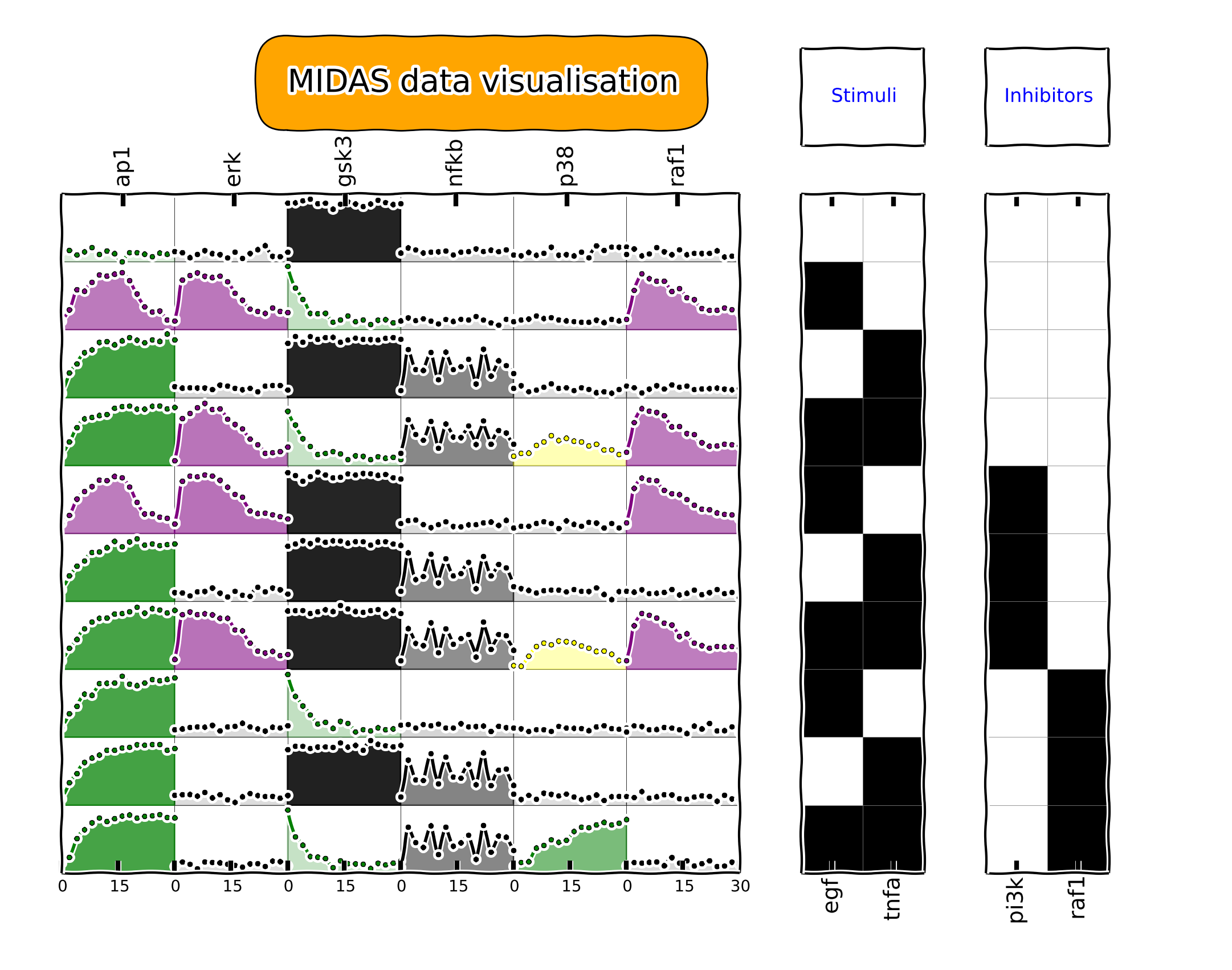
Figure 3: MIDAS data set visualised with cellnopt.core. Each row correspond to an experiment, that is a combination of stimuli and inhibitors (drug). An experiment is summarized by the two right panels where the x-axis contains the name of the stimuli and inhibitors and a black square means stimuli (or inhibitor) is on. The right panel contains the measurements made on each protein of interest over time. For example, the left bottom box gives us about 15 time points for the protein AP1 in the experimental conditions where EGF and TNFA receptors are stimulated and RAF1 is inhibited. The color in the boxes indicates the rough trend of the time series (e.g., green means activation is going up, the alpha transparency indicates the strength of the signals.).

2.2 cellnopt.wrapper

CellNOptR provides a set of R packages available on BioConductor website, which guarantees a minimal quality. Packages are indeed multi-platform and tested regularly. However, the functional approach that has been chosen limits somehow the user experience. In order to be able to use the Python language, we therefore decided to also provide a python wrapper. To do so, we used the RPY2 package. The cost for the implementation is reasonable: the R packages in CellNOptR relies on 16,000 lines of code (in R) and another 4,000 in C, while the final python wrappers requires 2000 lines of code including the documentation.

In addition to the wrappers, we also implemented a set of classes (or for each of the logical formalism) that encapsulate the R functions. The results is that cellnopt.wrapper (introduced in [CNO12]) provides a full access to the entire CellNOptR packages with an objected oriented approach.

A simple R script written with CellNOptR functions (to find the optimal model that fit the data) would look like:

1library(CellNOptR)2model = readSIF(CNOdata("PKN-ToyMMB.sif"))3data = CNOlist(CNOdata("MD-ToyMMB.csv"))4res = gaBinaryT1(data, model)5plotFit(res)6cutAndPlotResultsT1(model, res$bString, NULL, data)On the first line, we load the library. On the second and third lines, we read the PKN and MIDAS files. The optimisation is performed with a genetic algorithm (line 4). We plot the evolution of the objective function over time (line 5) and finally look at the individual fits (see Figure 4 for an example). Here below is the same code in Python using cellnopt.wrapper

1from cellnopt.wrapper import CNORbool2b = CNORbool(cnodata("PKN-ToyMMB.sif"),3             cnodata("MD-ToyMMB.csv"))4b.gaBinaryT1()5b.plotFit()6b.cutAndPlotResultsT1()The two code snippets are equivalent. The main difference appears to be that the first code is functional and the second is object-oriented. The value of the Python wrapping is that new classes can be derived, introspection of the data is possible and more importantly further manipulation of the results in Python is possible. Because an object-oriented approach is used in place of functional programming, the user interface is also simplified (no need to provide additional parameters).

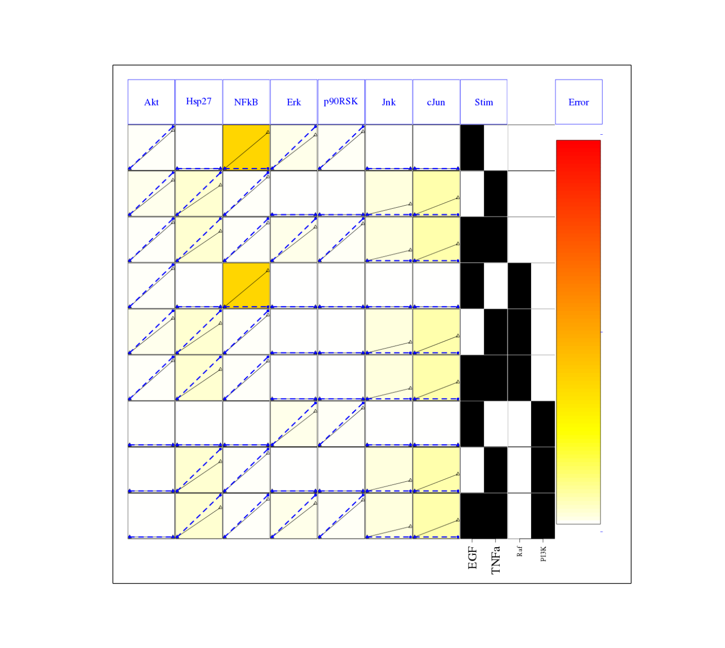
Figure 4: Fitness plot between the data and the best logical model. The plot is generated by CellNOptR via cellnopt.wrapper. See text for code snippet and more details.

Note that cellnopt.wrapper is designed to provide a full access to CellNOptR functionalities only. Yet, for end-users, it is often required to manipulate the PKN or MIDAS data structures. This was the main motivation to design cellnopt.core to complement CellNOptR.

2.3 cellnopt.core

2.3.1 PKN

The cellnopt.core package provides many tools to manipulate and visualise networks and MIDAS files. It is implemented in Python and makes use of standard scientific libraries including Pandas, Matplotlib and NetworkX.

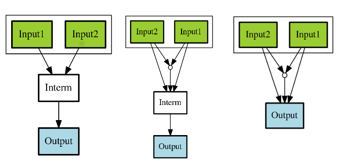
Figure 5: Toy example of a logic model (left panel). Logical and gates are represented with the small circles (middle). Logic-based models may also be compressed so as to simplify the network (right panel). Here the white node is not required. Removing it does not affect the logic in the network.

Coming back on the simple SIF example shown earlier, we could build it with the SIF class provided in cellnopt.core but will use another more advanced structure derived from the directed graph data structure provided by NetworkX. This class called CNOGraph has dedicated methods to design logic model. Although you can add nodes and edges using NetworkX methods, you can also add reactions as follows:

1from cellnopt.core import CNOGraph2c= CNOGraph()3c.add_reaction("Input2=Interm")4c.add_reaction("Input1=Output")5c.add_reaction("Interm=Output")6c._signals = ["Output"]7c._stimuli = ["Input1", "Input2"]8c.plot()where the = sign (A=B) indicates an activation. Inhibitions are encoded as !A=B, and as A^B=C and or as A+B=C. The results is shown in Figure 5 (left panel). By default all nodes are colored in white but list of stimuli, inhibitors or signals may be provided manually (line 6,7).

The training of the model to the data may also require to add AND gates, which is performed as follows:

1c.expand_and_gates()resulting in the model shown in Figure 5 (middle panel). You can also compress the network to remove nodes that do not change the logic as shown in Figure 5 (right panel):

c.compress()

On top of the graph data structure, we have also added the split/merge methods, which can be used to split/merge a protein node into its variants (e.g., AKT1 and AKT2 instead of just AKT). It can also be used in the context of mass-spectrometry where measurements of phosphorylation are made on each peptide individually rather than on the whole protein; number of peptides varies from a few to dozens of peptides per protein. Consider this simple example:

1c.split_node("Interm", ["Interm1", "Interm2"])2c.plot()The split/merge by hand would be tedious on large networks but is automated with the CNOGraph data structure taking into account AND gates and input edges (activation/inhibition). Once the PKN is designed, you can export it into SIF format:

1c.export2sif()You can also export the model into a SBML standard dedicated to logic models called SBMLQual, which keeps track of the OR and AND logical gates [CHA13].

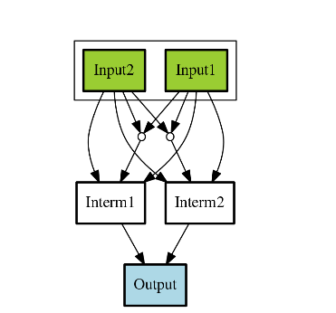
Figure 6: Starting from the middle panel of figure 5, CNOGraph data structure provides a method to split a node into several nodes (updating AND gates and edges automatically).

2.3.2 DATA

We discussed the MIDAS file format in Figure 3. CellNOptR provides tools to look at these data but cellnopt.core together with Pandas and Matplotlib gives more possiblities. Here is the code snippet to generate the Figure 3:

1from cellnopt.core import *2m = XMIDAS("MD-ToyPB.csv")3m.plot()The XMIDAS data structure contains 2 dataframes. The first one stores the experiments. It is a standard dataframe where each row is an experiment and each column is either a stimuli or an inhibitor. The second dataframe stores the measurements within a multi-index dataframe where the first dimension is the cell type, the second is the experiment name, and third is the time point. Each column corresponds to a protein. The following command shows the time-series of all proteins in the experiment labelled "experiment_0" (no stimuli, no inhibitors) as shown in Figure 7:

1>>> m.df.ix[’Cell’].ix[’experiment_0’].plot()2>>> m.experiments.ix[’experiment_0’]3egf       04tnfa      05pi3k:i    06raf1:i    07Name: experiment_0, dtype: int64

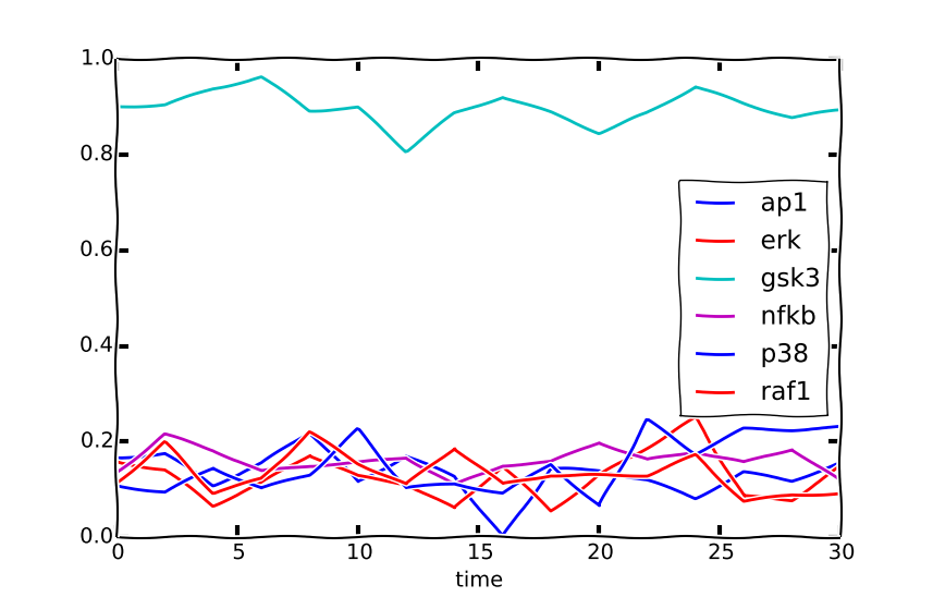
Figure 7: Example of time courses for a given combination of stimuli and inhibitors. This is the superposition of time series found in one row of Figure 3. One protein level (gsk3) is active while others are inactive when there is no stimuli and no inhibition)

One systematic issue when data is acquired is that it is stored in a non-standard format so additional scripts are required to translate into a complex data structure (e.g., MIDAS). Instead of rewriting codes, we can think about the data as a set of measurements defined by the list of stimuli and inhibitors, a time point and a value. We can then write one single script that transforms this list of measurements into a common MIDAS data structure. Here is an example:

from cellnopt.core import MIDASBuilderm = MIDASBuilder()e1 = Measurement("AKT", 0, {"EGFR":1}, {"AKT":0}, 0.1)e2 = Measurement("AKT", 5, {"EGFR":1}, {"AKT":0}, 0.5)e3 = Measurement("AKT",10, {"EGFR":1}, {"AKT":0}, 0.9)e4 = Measurement("AKT", 0, {"EGFR":0}, {"AKT":0}, 0.1)e5 = Measurement("AKT", 5, {"EGFR":0}, {"AKT":0}, 0.1)e6 = Measurement("AKT",10, {"EGFR":0}, {"AKT":0}, 0.1)for e in [e1,e2,e3,e4,e5,e6]:...     m.add_measurement(e)m.export2midas("test.csv")m.xmidas.plot()There are many more functionalities available in cellnopt.core especially to visualise the networks by adding attribute on the edges or nodes, described within the online documentation.

2.4 Discussion and future directions

In order to call the CellNOptR functionalities within Python, we decided to use RPy2. There are 16,000 lines of R code in CellNOptR and 4,000 lines of C code, that could not be re-used within Python without being altered. However, the C code is called by the R functions and therefore does not need any wrapping functions. Even though the wrapping could be written following RPy2 documentation, however, we had to take into account some considerations. First, we did not want to rewrite the documentation. The simplest solution we found was to implement a decorator (called Rsetdoc) that appends the R documentation to the python docstring. Another issue is that it is non-trivial for the end-user to figure out where to access to the R objects inside the python function. Consequently, we wrote another decorator (Rnames2attributes) that transforms the R objects into read-only attribute. So, our wrapping could be as simple as:

@Rsetdoc@Rnames2attributesdef readSIF(filename):    return rpack_CNOR.readSIF(filename)With a straightforward usage, especially for those familiar with the R commands (same function name):

from cellnopt.wrapper import readSIFs = readSIF(cnodata("PKN-ToyMMB.sif"))s.interMat<Matrix - Python:0x6c0a9e0 / R:0x68f7740>[-1.000000, 0.000000, 0.000000, ...Yet, the design and maintenance of the wrapper has a cost. From the development point of view, we have to keep in mind that the wrapper and the R code have to be closely managed either by the same developer or team of developers so that the two codes are maintained and updated synchronously. The second issue is that a high-level interface such as RPy2 may have a cost on performance. This is not apparent on a simple script with only a few function calls, but may be obvious when calling a function a million times (e.g., to perform an optimisation of a CellNOptR objective function). Although not as elegant, an alternative to RPy2 is to use the subprocess Python module, which could call a static R pipeline.

3 BioServices

3.1 Context and motivation

In order to construct the PKN required by CellNOpt, we need to access to web resources such as signalling pathways or protein identifiers. Many resources can be accessed to in a programmatic way thanks to web services. Building applications that combine several of them would benefit from a single framework. This was the main reason to develop BioServices, which is a comprehensive Python framework that provides programmatic access to major bioinformatics web services (e.g., KEGG, UniProt, BioModels, etc.).

Two protocols are used to access to web services (i) REST (Representational State Transfer) and (ii) SOAP (Simple Object Access Protocol). REST has an emphasis on readability and each resource corresponds to a unique URL. Operations are carried out via standard HTTP methods (e.g. GET, POST). SOAP uses XML-based messaging protocol to encode request and response messages using WSDL (Web Services Description Language).

In order to build applications that integrate several web services, one needs to have expertise in (i) HTTP requests, (ii) SOAP protocol, (iii) REST protocol, (iv) XML parsing to consume the XML messages and (v) related bioinformatics fields. Consequently, the composition of workflows or design of external applications based on several web services can be challenging. BioServices hides the technical aspects of accessing to web services thereby giving access to a service in a few lines of codes.

3.2 Approach and Implementation

For developers, there is a class dedicated to REST protocol, and a class dedicated to WSDL/SOAP protocol. With these classes in place, it is then straightforward to create a class dedicated to new web service given its URL. Let us consider WikiPathway [WP09], which uses a WSDL protocol:

1from bioservices import WSDLService2url ="http://www.wikipathways.org/"3url += "wpi/webservice/webservice.php?wsdl"4class WikiPath(WSDLService):5   def __init__(self):6     super(WikiPath, self).__init__("WP", url=url)7wp = WikiPath()8wp.methods # or wp.serv.methodsAll public methods are shown in the wp.methods attribute. A developer can then access directly to those methods or wrap them to add robustness, quality and documentation. Let us now use this service to obtain a list of signalling pathways that contains the protein MTOR:

1from bioservices import WikiPathway2s = WikiPathway()3pathways = s.findPathwaysByText("MTOR")We can then retrieve a particular signalling pathway and look at it (see Figure 8) to complete our prior knowledge:

1# Get a SVG representation of the pathway2image = w.getColoredPathway("WP2320")

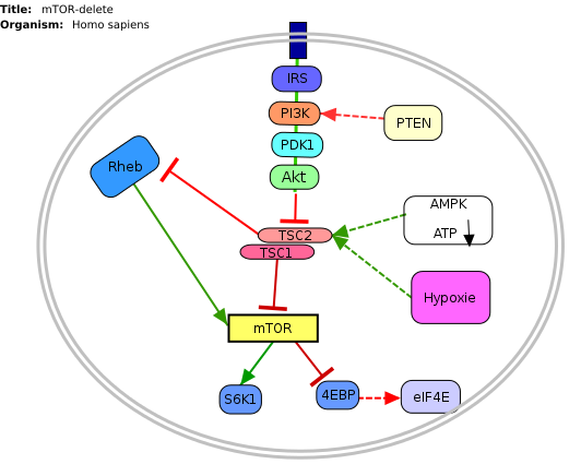
Figure 8: Image obtained from WikiPathway showing a signalling pathway that contains the mTOR protein.

3.3 Combining BioServices with standard scientific tools

In general, BioServices does not depend on scientific librairies such as Pandas so as to limit its dependencies. However, there are a few experimental methods with a local import so that Pandas is not required during the installation. In the next example, we will use one of these experimental methods. UniProt service [UNI14] is useful in CellNOpt for protein identification and mapping. Let us use it to extract the sequence length of those proteins. We will then study its distribution. Assuming you have a list of valid identifiers, just type:

1# we assume you have a list of entries.2from bioservices import UniProt3u = UniProt()4u.get_df(entries)Note that the method get_df uses Pandas: it returns a dataframe. One of the column contains the sequence length. The sequence length distribution can then be fitted to a SciPy distribution [SCIPY] (using a simple package called fitter, which is available on PyPi):

1data = df[df.Length<3000].Length2import fitter3f = fitter.Fitter(data, bins=150)4f.distributions = [’lognorm’, ’chi2’, ’rayleigh’,5    ’cauchy’, ’invweibull’6f.fit()7f.summary()In this example, it appears that a log normal distribution is a very good guess as shown in Figure 9. Code to get the entries and regenerate this results is available within BioServices documentation as an IPython [IPYTHON] notebook.

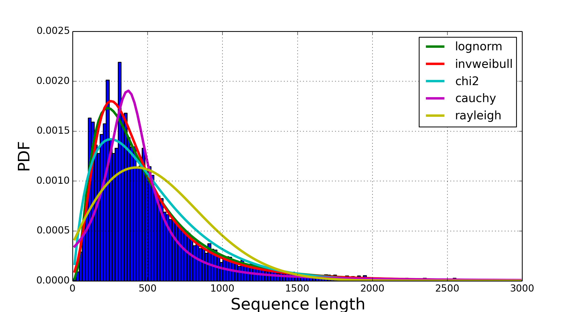
Figure 9: Distribution of the length of 20,000 protein sequence (human). Distribution was fitted to 80 distributions using SciPy distribution module and fitter package. A log normal distribution with parameters fits the length distribution. See code snippet in the text.

REST	ArrayExpress, BioMart, ChEMBL, KEGG, HGNC, PDB, PICR, PSICQUIC, QuickGO, Rhea, UniChem, UniProt, NCBIBlast, PICR, PSICQUIC
WSDL/SOAP	BioModel, ChEBI, EUtils, Miriam, WikiPathway, WSDbfetch

TABLE II: Web services accessible from BioServices (release 1.2.6).

3.4 Status and future directions

BioServices provides a comprehensive access to bioinformatics web services within a single Python library. See Table I for the current list of services.

The previous example lasts about 20 minutes depending on the network speed. There are faster way to obtain such information like downloading the database or flat files. Yet, one need to consider that such files are large (500Mb for UniProt) and that they may be updated regularly. You may also want to use several services, which means several flat files. Within a pipeline, you may not want to provide a set of 500Mb files. In BioServices, the idea is that you do not necessarily want to download flat files and are willing to wait for the requests. Future directions of BioServices are two-fold. One is to provide new web services depending on the user requests and/or contributions. The second aspect is to make the core functionalities of BioServices faster. This has been recently achieved with (i) the usage of the requests package over the urllib2 module (30% gain) and the buffering or caching of requests to speed up repetitive requests (also based on the requests package).

4 Conclusions

In this paper, we presented cellnopt.wrapper that provides a Python interface to CellNOptR software. We discussed how and why RPy2 was used to develop this wrapper. We then presented cellnopt.core that provides a set of tools to manipulate input data structures required by CellNOptR (MIDAS and SIF formats amongst others). Visualisation tools are also provided and the package is linked to Pandas, NetworkX and Matplotlib librairies making user and developer experience easier and more dynamic. Note that Python is also used to connect CellNOpt to Answer Set Programming (with the Caspo package [ASP13]) and to heuristic optimisation methods ([EGE14]).

We also briefly introduced BioServices Python package that allows a programmatic access to web services used in life sciences. The main interests of BioServices are (i) to hide technical aspects related to web resource access (GET/POST requests) so as to foster the integration of new web services (ii) to put within a single framework many web services.

Source code and extensive on-line documentation are provided on http://pypi.python.org/pypi website (bioservices, cellnot.wrapper, cellnopt.core packages). More information about CellNOptR are available on http://www.cellnopt.org.

5 Acknowledgment

Authors acknowledge support from EU BioPreDyn FP7-KBBE grant 289434.

References

- [ASP13] Guziolowski et al. Exhaustively characterizing feasible logic models of a signaling network using Answer Set Programming Bioinformatics(2013) 29 (18) 2320-2326
- [EGE14] J. Egea et al. MEIGO: an open-source software suite based on metaheuristics for global optimization in systems biology and bioinformatics BMC Bioinformatics 2014, 15:136
- [UNI14] The UniProt Consortium. Nucleic Acids Res. 42: D191-D198 (2014).
- [COK13] T. Cokelaer, D. Pultz, L.M. Harder, J. Serra-Musach and J. Saez-Rodriguez BioServices: a common Python package to access biological Web Services programmatically Bioinformatics, 29 (24) 3241-3242 (2013)
- [WP09] T. Kelder, AR. Pico, K. Hanspers, MP. van Iersel, C. Evelo, BR. Conklin. Mining Biological Pathways Using WikiPathways Web Services. PLoS ONE 4(7) (2009). doi:10.1371/journal.pone.0006447
- [CNO12] C. Terfve, T. Cokelaer, A. MacNamara, D. Henriques, E. Goncalves, M.K. Morris, M. van Iersel, D.A. Lauffenburger, J Saez-Rodriguez. CellNOptR: a flexible toolkit to train protein signaling networks to data using multiple logic formalisms. BMC Systems Biology, 2012, 6:133
- [CHA13] C. Chaouiya et al. SBML qualitative models: a model representation format and infrastructure to foster interactions between qualitative modelling formalisms and tools BMC Systems Biology 2013, 7:135
- [IPYTHON] F. Pérez and B. E. Granger. IPython: A system for interactive scientific computing. Computing in Science & Engineering, 9(3):21-29, 2007. http://ipython.org/
- [HUN07] J. D. Hunter. Matplotlib: A 2d graphics environment. Computing in Science & Engineering, 9(3):90-95, 2007. http://matplotlib.org
- [SCIPY] E. Jones, T. E. Oliphant, P. Peterson, et al. SciPy: Open source scientific tools for Python, 2001-. http://www.scipy.org
- [MCK10] W. McKinney Data Structures for Statistical Computing in Python in Proceedings of the 9th Python in Science Conference, p 51-56 2010
- [MIDAS] J. Saez-Rodriguez, A. Goldsipe, J. Muhlich, L. Alexopoulos, B. Millard, D. A. Lauffenburger, P. K. Sorger, Flexible Informatics for Linking Experimental Data to Mathematical Models via DataRail. Bioinformatics, 24:6, 840-847 (2008).
- [SAEZ] J. Saez-Rodriguez et al. Discrete logic modelling as a means to link protein signalling networks with functional analysis of mammalian signal transduction Mol. Syst. Biol. (2009), 5, 331
- [MAC12] A. MacNamara, C. Terfve, D. Henriques, B. Petilde{n}alver Bernabacute{e}, and J. Saez-Rodriguez State–time spectrum of signal transduction logic models 2012 Phys. Biol. 9 045003
- [IDE01] T. Ideker, T. Galitski, L. Hood. A new approach to decoding life: systems biology. Annual Review of Genomics and Human Genetics. 2001;2:343–372.
- [KIT02] H. Kitano. Systems biology: a brief overview. Science. 2002;295(5560):1662–1664.
- [ARI08] A.A. Hagberg, D.A. Schult and P.J. Swart, Exploring network structure, dynamics, and function using NetworkX in Proceedings of the 7th Python in Science Conference (SciPy2008), pp. 11–15, (2008)
- [HAUPT] S. Haupt, M. Berger, Z. Goldberg, Y. Haupt Apoptosis - the p53 network Journal of Cell Science, (2003), 116, 4077-4085.