DESIGN AND PERFORMANCE OF THE X-RAY POLARIMETER X-CALIBUR

Abstract

X-ray polarimetry promises to give qualitatively new information about high-energy astrophysical sources, such as binary black hole systems, micro-quasars, active galactic nuclei, neutron stars, and gamma-ray bursts. We designed, built and tested a X-ray polarimeter, X-Calibur, to be used in the focal plane of the balloon-borne InFOC$\mu$S grazing incidence X-ray telescope. X-Calibur combines a low-Z scatterer with a CZT detector assembly to measure the polarization of $20-80\,\rm{keV}$ X-rays making use of the fact that polarized photons scatter preferentially perpendicular to the electric field orientation. X-Calibur achieves a high detection efficiency of $\simeq 80\%$. The X-Calibur detector assembly is completed, tested, and fully calibrated. The response to a polarized X-ray beam was measured successfully at the Cornell High Energy Synchrotron Source. This paper describes the design, calibration and performance of the X-Calibur polarimeter. In principle, a similar space-borne scattering polarimeter could operate over the broader $2-100\,\rm{keV}$ energy band.

; ; ;

1 Introduction

Only the most violent objects in the universe are capable of producing high-energy particles in non-thermal acceleration processes and emit photons with energies in the X-ray band and above. Spectral and morphological studies in the X-ray and gamma-ray bands have become established tools to study the non-thermal emission processes of various astrophysical sources Seward & Charles [2010]. However, many of the regions of interest (black hole vicinities, formation zones of relativistic jets, etc.) are too small to be spatially resolved with current and future instruments. Spectro-polarimetric X-ray observations are capable of providing additional information – namely (i) the energy-resolved fraction of linear polarization (e.g. what fraction of emission is polarized), and (ii) the projected orientation of the polarization plane (defined by the electric field vector of the photon) with respect to the emitting source. Various emission mechanisms of compact objects lead to comparable spectral signatures, but would differ in the polarization characteristics. The measurements of polarization properties would therefore help to constrain the geometry of the inner regions of relativistic plasma jets, mass-accreting black holes (BHs) and neutron stars Lei et al. [1997]; Krawczynski et al. [2011].

So far, only a few space-borne missions have successfully measured polarization in the X-ray regime. The Crab nebula is the only source for which X-ray polarization has been established with a high level of confidence. In measurements with the OSO-8 satellite, the Crab exhibits a polarization fraction of $20\%$ at energies of $2.6-5.2\,\rm{keV}$ and a direction angle of $30^{\circ}$ with respect to the X-ray jet observed in the nebula Weisskopf et al. [1978]. At energies above $100\,\rm{keV}$, measurements resulted in a polarization fraction of $46\%\pm 10\%$ with the direction aligned with the jet Dean et al. [2008]; Forot et al. [2008]. A second astrophysical source emitting polarized X-rays was identified recently. INTEGRAL observations of the X-ray binary Cygnus X-1 indicate a high fraction of polarization of $(67\pm 30)\%$ in the $400\,\rm{keV}-2\,\rm{MeV}$ band, whereas a $20\%$ upper limit was derived for the $250-400\,\rm{keV}$ band Laurent et al. [2011]. Various authors have reported tentative evidence for polarized hard X-ray/soft gamma-ray emission from different gamma-ray bursts Coburn & Boggs [2003]; Kalemci et al. [2007]; Yonetoku et al. [2011]; Kostelecky & Mewes [2013]. However, all of these detections have somewhat marginal significance, possibly being impacted by unknown systematic effects in their respective instrumentation.

Model predictions of polarized emission for various source types lie slightly below the sensitivity of the past OSO-8 mission, making future, more sensitive polarimetry missions particularly interesting. However, there are currently no dedicated missions in orbit that are capable of measuring X-ray polarization fractions in the $<10\%$ regime, a requirement to study the corresponding emission mechanisms for a variety of astrophysical source classes (see Sec. 2). More recently, various experiments have been proposed that could change the situation as they combine broadband sensitivity with a high detection efficiency. The proposed polarimeters use focusing mirrors to collect photons from the source. Photoelectric effect polarimeters, like the Gravity and Extreme Magnetism SMEX (GEMS) mission Hill et al. [2012] and XIPE Soffitta et al. [2013], track the direction of photo electrons ejected in photoelectric effect interactions of the X-rays. The ASTRO-H mission (to be launched in 2015) will carry the Soft Gamma-Ray Imager. The detector combines an X-ray and gamma-ray collimator with a Si scatterer and CdTe absorber. The mission will be able to do scattering polarimetry at $E>50\,\rm{keV}$ energies Tajima et al. [2010]. Our group is working on a proposal of the space borne scattering polarimeter PolSTAR which uses a lower-Z LiH stick as a scatterer to enable the detection of $3-80\,\rm{keV}$ X-rays. The PolSTAR concept will be described in a forthcoming paper. Missions like GEMS, PolSTAR and XIPE aim at obtaining $1\%$ minimum detectable polarization fractions, see Eq. (4), for mCrab sources. These missions would allow very high-signal-to-noise detections of bright galactic sources (e.g. Cyg X-1, GRS 1915+105, Her X-1) and could detect $\sim 1\%$ polarization fractions for extra-galactic sources (e.g. NGC 4151).

Scattering polarimeters detect the direction into which photons scatter when interacting in the detector. Although different scattering processes dominate at different energies (coherent scattering below a few keV, Thomson scattering at intermediate energies, and Compton scattering at energies $>20\,\rm{keV}$), all scattering processes share the property that the photons scatter preferentially perpendicular to the polarization plane (electric field vector) of the incoming photon. For example, the angular dependence of Compton scattering processes is given by the Klein-Nishina cross section Evans [1955]:

$$\frac{\rm{d}\sigma}{\rm{d}\Omega}=\frac{r_{0}^{2}}{2}\frac{k_{1}^{2}}{k_{0}^{2}}\left[\frac{k_{0}}{k_{1}}+\frac{k_{1}}{k_{0}}-2\sin^{2}\theta\cos^{2}\eta\right],$$ (1)

where $\eta$ is the angle between the electric vector of the incident photon and the scattering plane, $r_{0}$ is the classical electron radius, $\bf{k}_{0}$ and $\bf{k}_{1}$ are the wave-vectors before and after scattering, and $\theta$ is the scattering angle. The azimuthal distribution of scattered events shows a sinusoidal modulation with a $180^{\circ}$ periodicity and a maximum at $\pm 90^{\circ}$ to the preferred electric field direction of a polarized X-ray signal.

In this paper we describe the design and performance of a scattering polarimeter, X-Calibur. The polarimeter utilizes a plastic scintillator as scatterer which can scatter $E>20\,\rm{keV}$ X-rays efficiently. This is ideal for the operation on a balloon where the energy threshold is well matched to the low energy cutoff of the transmissivity caused by the residual atmosphere above the balloon altitude of 125,000 feet. An assembly of Cadmium Zinc Telluride (CZT) detectors surrounds the scintillator in order to record the azimuthal distribution of the scattered photons, allowing one to reconstruct the polarization properties of the incoming X-ray beam. The background of charged particles and high-energy photons is suppressed by an active CsI shield.

The paper is structured as follows. Section 2 gives a brief overview over the scientific potential of hard X-ray polarimetry. The design of the X-Calibur polarimeter is described in Sec. 3. The data analysis methods are described in Sec. 4, followed by an outline of the simulation procedure in Sec. 5. Section 6 describes the calibration and characterization studies of the CZT detectors. Measurements with the assembled X-Calibur polarimeter to characterize the scattering scintillator and the shield are described in Sec. 7. Polarization measurements with X-Calibur are described in Sec. 8. The paper ends with a summary and outlook in Sec. 9. The X-Calibur data presented in this paper were taken (i) in a laboratory environment at Washington University, (ii) at the Cornell High Energy Synchrotron Source (CHESS), and (iii) in Ft. Sumner, NM, during a preparation campaign for an upcoming balloon flight.

2 Scientific Potential

This section discusses the scientific potential for a scattering polarimeter such as X-Calibur from a balloon platform. X-rays from cosmic sources can be polarized owing to the anisotropy in the source geometry and/or the emission characteristics of various processes Lei et al. [1997]. Non-thermal emission, like synchrotron radiation, results in a large polarization fraction $r$. Synchrotron emission will result in linearly polarized photons with their electric fields oriented perpendicular to the magnetic field lines (projected); the observed polarization map can therefore be used to trace the magnetic field structure of the source, a common practice in radio and optical polarimetry. An electron population with a spectral energy distribution of $\rm{d}N/\rm{d}E\propto E^{-p}$ emitting in a uniform magnetic field will lead to an observable fraction of polarization of Korchakov & Syrovatskii [1962]:

$$r_{\rm{sync}}=\frac{p+1}{p+7/3},\quad\rm{with}\,(p+3)=\frac{\alpha+1}{\alpha+5/3}.$$ (2)

Here, $\alpha$ is the index of the X-ray power law spectrum. An observed polarization fraction close to this limit can therefore be interpreted as an indication of a highly ordered magnetic field since non-uniformities in the magnetic field will reduce $r_{\rm{sync}}$. The polarized synchrotron photons can in turn be inverse-Compton scattered by relativistic electrons – weakening the fraction of polarization (but not erasing it) and imprinting a scattering angle dependence to the observed fraction of polarization Krawczynski [2012a]. Such inverse-Compton signals will usually (but not always) appear in hard gamma-rays, where polarimetry is difficult, due to multiple scattering in pair production detectors. Another important mechanism for polarizing photons is Thomson scattering which creates a polarization perpendicular to the scattering plane Rybicki & Lightman [1991]. Curvature radiation is polarized, as well. The scientific potentials of spectro-polarimetric observations over the broadest possible energy range are summarized below; more detailed discussions can be found in Krawczynski et al. [2011] and Lei et al. [1997].

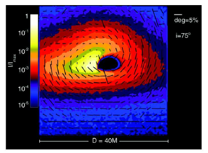
Figure 1: Ray-traced image of direct radiation from a thermal disk around a BH including returning radiation (observer located at an inclination angle of $75^{\circ}$, gas on the left side of the disk moving toward the observer causing the characteristic increase in intensity due to relativistic beaming). The image is adopted from Schnittman & Krolik [2009]. The observed intensity is color-coded on a logarithmic scale and the energy-integrated polarization vectors are projected onto the image plane with lengths proportional to the fraction of polarization.

Binary black hole systems. Particle scattering in a Newtonian accretion disk surrounding a BH will lead to the emission of polarized X-rays. Relativistic aberration and beaming, gravitational lensing, and gravito-magnetic frame-dragging will result in an energy-dependent fraction of polarization since photons with higher energies originate closer to the BH than the lower-energy photons Connors & Stark [1977]. Schnittman & Krolik [2009] calculate the expected polarization signature including (i) the effects of deflection of photons emitted in the disk by the strong gravitational forces in the regions surrounding the BH and (ii) re-scattering these photons by the accretion disk Schnittman & Krolik [2009, 2010]. The resulting effect is a swing in the polarization direction from being horizontal at low energies to vertical at high energies, i.e., parallel to the spin axis of the BH. Spectro-polarimetric observations can therefore be used to constrain the mass and spin of the BH Schnittman & Krolik [2009], as well as the inclination of the inner accretion disk and the shape of the corona Schnittman & Krolik [2010], see Fig. 1. In principle, X-ray polarization can also be used to test General Relativity in the strong gravity regime Krawczynski [2012b].

Pulsars. High-energy particles in pulsar magneto-spheres are expected to emit synchrotron and/or curvature radiation which are difficult to distinguish from one another, solely based on the observed photon energy spectrum. However, since the orbital planes for accelerating charges that govern these two radiation processes are orthogonal to each other, their polarized emission will exhibit different behavior in position angle and polarization fraction as functions of energy and the rotation phase of the pulsar Dean et al. [2008]. An illustration of the models of phase dependence of the X-ray/gamma-ray polarization signatures in pulsars can be found in Dyks et al. [2004]. In magnetars, the highly-magnetized cousins of pulsars, polarization-dependent resonant Compton up-scattering is a leading candidate for generating the observed hard X-ray tails Baring & Harding [2007]. In both these classes, phase-dependent spectro-polarimetry can probe the emission mechanism, and provide insights into the magnetospheric locale of the emission region.

Cyclotron lines arising from transitions between Landau levels in intense magnetic fields that occur in the polar regions of neutron stars and magnetars are polarized. Also, the absorption scattering cross-sections from the Landau levels are dependent on the polarization state of the X-rays, so that the radiative transfer through such plasma will lead to a polarization of the emergent radiation. The first such cyclotron feature was observed by Truemper et al. [1978] in Her X-1 and is interpreted as due to an absorption line around $40\,\rm{keV}$ Staubert et al. [2007]. Such features allow an estimate of the magnetic field strength Coburn et al. [2002]. Observations of polarized X-rays will strongly confirm that these features are indeed due to cyclotron lines in magnetic fields of $3-5\times 10^{12}\,\rm{G}$. A detailed discussion of the theoretical aspects of cyclotron radiation is given in Semionova et al. [2010].

Pulsar wind nebulae. The compact object (e.g. pulsar) resulting from a previous supernova explosion can be surrounded by a synchrotron emitting nebula. The nebula extends far beyond the magneto-sphere of the central pulsar, but its emission is believed to be driven by the pulsar which injects relativistic electrons/positrons that are further shock accelerated in the nebula. Spectro-polarimetric observations can be used to constrain the magnetic field and particle populations in such pulsar wind nebulae – such as the Crab nebula, the leading driver for this field of X-ray polarimetry. Given the more compact emission regions at high energies, these objects potentially show a higher polarization fraction at hard X-rays as compared to soft X-rays, reflecting the contrast between jet and more diffuse nebular contributions Forot et al. [2008].

Supernova remnants. Supernova remnants (SNRs) present an opportunity to perform X-ray polarimetry, as well. The remnants possess tangled magnetic fields on large scales in their interiors, as is evidenced in the classic radio polarization map of the Crab nebula Velusamy [1985]. Both, radio and X-ray signals, are believed to be due to synchrotron emission, and so it is reasonably presumed that X-ray emission from SNRs should be significantly polarized. The X-ray spectra of such remnants are typically steeper than spectra in the radio, which leads to the expectation of higher polarization fractions in the X-ray band. Yet, since the electrons generating X-rays will diffuse on larger spatial scales than their radio-emitting counterparts do, the X-ray signals should capture the field morphology on larger scales. It may or may not be more coherent than the field structure on smaller (radio) scales. Due to instrumental limitations in angular resolution at X-ray energies, however, it will not be possible to resolve individual regions – depending on the angular size of the remnant. The observational challenge will therefore be to overcome the competition between compact regions causing highly polarized emission on one hand, and on the other hand an averaging effect of different emission regions with different orientations of their magnetic fields. An example of expectations for the SNR synchrotron polarization properties can be found in Bykov et al. [2009].

Relativistic jets in active galactic nuclei. Relativistic electrons in jets of active galactic nuclei (AGN) emit polarized synchrotron radiation at radio/optical wavelengths. The same electron population is believed to produce hard X-rays by inverse-Compton scattering off a photon field. Simultaneous measurements of the polarization angle and the fraction of polarization in the radio to hard X-ray band could help to disentangle the following scenarios: (i) If the electrons mainly up-scatter the co-spatial synchrotron photon field (synchrotron self Compton), the polarization of the hard X-rays is expected to track the polarization at radio/optical wavelengths Poutanen [1994]. The fraction of X-ray polarization could be close to the fraction of polarization of the synchrotron emission measured in the radio/optical bands and the polarization directions between radio, optical and X-rays should be identical. (ii) If the electrons dominantly up-scatter an external photon field (external Compton, e.g. photons of the cosmic microwave background or from the accretion disk surrounding the super-massive black hole) the hard X-rays will have a relatively small ($<$10%) fraction of polarization McNamara et al. [2009]. Hadronic jet emission models for low-synchrotron-peaked AGN, on the other hand, predict an even higher fraction of polarization at high energies, compared to the leptonic SSC models Zhang & Böttcher [2013].

Polarization also allows one to test the structure of the magnetic field of the jet. Particles accelerated in a helical field which are moving through a standing shock can cause an X-ray synchrotron flare with a continuous (in time) swing in polarization direction. Such an event was observed from BL Lacertae at optical wavelengths Marscher et al. [2008].

Gamma-ray bursts. Gamma-ray bursts are believed to be connected to hyper-nova explosions and the formation/launch of relativistic jets Woosley [1993]. As in the case of the jets in AGN, the structure of their jets and the particle distribution responsible for gamma-ray bursts can be revealed by X-ray polarization measurements Kostelecky & Mewes [2013]. The X-ray emission of a gamma-ray burst, however, usually lasts for only a few minutes at most, so that rapid follow-up observations in the X-ray band below $30\,\rm{keV}$ would be the main challenge for studying their polarization properties.

On a one-day balloon flight, we would achieve $5-15\%$ MDPs, see Eq. (4), for between 1 and 4 sources. For the Crab, the phase resolved polarimetry would allow us to decide between emission models. For Cyg X-1 and GRS 1915+105 we could test corona models, and for Her X-1, we could get a first estimate of the polarization fraction of the X-ray emission.

3 Design of X-Calibur

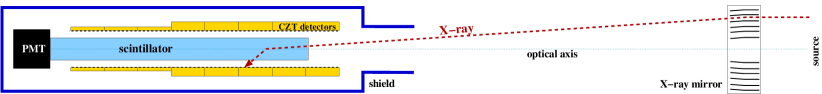
Figure 2: Schematic view of the functionality of X-Calibur (not to scale). X-rays from an astrophysical source are focused with a grazing incidence mirror onto the scattering rod of the polarimeter. The scattered X-ray is recorded in one of the surrounding CZT detectors. The polarimeter is embedded by a shield to suppress background of particles not originating from the mirror.

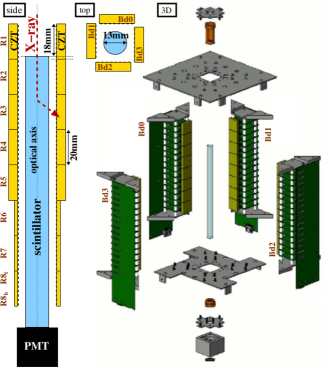
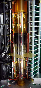
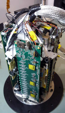
Figure 3: Design of the X-Calibur polarimeter. Left: Schematic illustration. Side view: incoming X-rays Compton-scatter in the scintillator rod (aligned with the optical axis, read out by a PMT) and are subsequently photo-absorbed in one of the surrounding CZT detectors ($8\times 8$ pixels each, see Fig. 4). A group of four detectors surrounding the scintillator at a given depth are referred to as ring (R1 to R8). Each ring can be further divided into top and bottom sub rings, as illustrated for ring R8. Top view: Detector ring viewed along the optical axis, looking into the X-ray beam. The polarization signature is imprinted in the azimuthal scattering distribution (see Fig. 6, top, for more details). The four sides of detectors are referred to as boards (Bd0 to Bd3), each board comprising all eight detectors per side. 3D view (‘exploded’): four sides of detector columns (Bd0 to Bd3) surround the central scintillator rod – covering the whole range of azimuthal scattering angles. Middle: Partly assembled polarimeter with two detector sides removed for better visibility. The red wires provide the high voltage to the detectors. The read-out electronics is stacked at the backside of the detectors. Right: Fully assembled polarimeter (flipped upside-down: X-ray entering from the bottom).

ID	Serial-No.	Date	$C_{\rm{ch}}$	$C_{\rm{wu/ft}}$
Endicott 5 mm
EN51	672992-01	01/11	0/5	0/5
EN52	672992-02	01/11	1/5	1/5
EN53	672992-03	01/11	2/5	2/5
EN54	672992-04	01/11	3/5	3/5
EN55	672994-04	02/11	0/4	0/4
EN56	672994-03	02/11	1/4	1/4
EN57	672994-02	02/11	2/4	2/4
EN58	672994-01	02/11	3/4	—
Creative Electron 5 mm
CE51	721613	03/11
QuikPak 5 mm
QP51	3627	03/11	—	3/4
QP53	3611	03/11	—	—
QP54	3834	03/11	3/1	3/1
QP56	6292	03/11	0/1	0/1
QP57	6345	03/11	2/1	2/1
QP58	721c602	03/11	1/1	1/1
QP513	6886	04/12	0/3	0/3
QP514	6977	04/12	2/3	2/3
QP516	10814	04/12	2/2	2/2
QP517	10819	04/12	0/2	0/2
QP518	10829	04/12	1/2	1/2
QP519	10847	04/12	3/3	3/3
QP520	10848	04/12	3/2	3/2
QP521	10860	04/12	1/3	1/3
Endicott 2 mm
EN21	674326-01	02/11	0/6	0/8
EN22	674327-01	02/11	2/8	2/8
EN23	674328-01	02/11	2/6	2/6
EN24	674328-02	02/11	0/8	0/6
EN25	674329-01	02/11	—	—
EN26	674330-01	02/11	1/6	1/6
EN27	674331-01	02/11	3/6	—
EN28	674332-01	02/11	—	3/8
Creative Electron 2 mm
CE21	2180	03/11	0/7	0/7
CE22	720612	03/12	3/8	3/6
CE23	720511	03/12	1/8	1/8
CE24	721541i	03/12	1/7	1/7
CE25	06172A	03/12	2/7	2/7
CE26	726712	03/12	3/7	3/7

Table 1: CZT detector sample. ID as in this paper (two letters for the company, index for the detector thickness $[\rm{mm}]$, and a number), serial number, date of delivery [MM/YY], and position in polarimeter [Bd/ring] for the configurations $C_{\rm{ch}}$ and $C_{\rm{wu/ft}}$ (see Fig. 6).

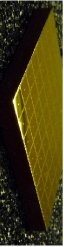
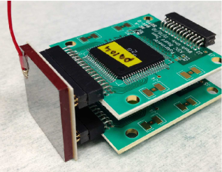
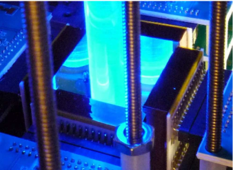
Figure 4: Definition of a detector ‘ring’. Left: $2\times 2\times 0.2\,\rm{cm}^{3}$ CZT detector with 64 pixels (anode side). Middle: $2\times 2\times 0.2\,\rm{cm}^{3}$ CZT detector bonded to a ceramic chip carrier which is plugged into 2 ASIC readout boards. The high-voltage cable is glued to the detector cathode (red wire). Right: Four CZT detectors surrounding the scintillator (blueish glow) form a unit referred to as ‘ring’ – covering the whole $360^{\circ}$ azimuthal scattering range with $4\times 8=32$ pixels. The whole polarimeter is equipped with eight rings.

The balloon-borne version of X-Calibur is a low-Z Compton scattering polarimeter that will allow one to measure polarization fractions in the $20-80\,\rm{keV}$ band down to the percentage level. X-Calibur will be used in the focal plane of the X-ray mirror of the InFOC$\mu$S telescope with a field-of-view of $10\,\rm{arcmin}$; X-Calibur does not provide imaging capabilities. Owing to the fact that a grazing incidence mirror reflects only under very shallow angles, it changes the polarization properties of X-rays by less than $1\%$ Katsuta et al. [2009]. The advantages of the X-Calibur design can be described as follows. (i) A high detection efficiency is achieved, using roughly $80\%$ of photons impinging on the polarimeter. (ii) The use of a focusing optics instead of a large detector volume results in a compact instrument design that can be shielded efficiently – strongly reducing the background level. (iii) The continuous rotation of the polarimeter strongly reduces possible systematic effects that can hamper non-rotating polarimeters due to asymmetric azimuthal detector responses. These characteristics, as outlined in the following sections, make it a well-suited experiment to study several sources mentioned in Sec. 2 in a one-day balloon flight. The energy-dependent detection efficiency of the polarimeter depends on (i) the effective area and point-spread function of the X-ray mirror, (ii) the fraction of scatterings compared to competing interactions such as photo-absorption, and (iii) the geometrical detector coverage to record a high fraction of scattered X-rays (minimization of possible escape paths) Guo et al. [2010]. This section describes the overall design of the polarimeter, as well as the characteristics of its individual components.

3.1 Design

The conceptual design of the X-Calibur polarimeter is illustrated in Figures 2 and 3. A low-Z scintillator rod aligned with the optical axis of the telescope is used as Compton-scatterer – leading to a polarization-dependent azimuthal scattering distribution that is recorded by the surrounding assembly of CZT detectors. The azimuthal distribution is resolved by $4\times 8=32$ pixels for each of the $64$ depth bins along the optical axis. Detailed information on the simulations to optimize the X-Calibur design (as presented in this paper) can be found in Krawczynski et al. [2011] and Guo et al. [2013].

Throughout the paper, we refer to a detector ring as a set of four CZT detectors surrounding the scintillator rod on four sides at a given depth along the optical axis (see Fig. 4, right). Ring R1 is situated at the polarimeter entrance (top in Fig. 3, left), and ring R8 is situated at its rear end. Each ring covers the whole $360^{\circ}$ azimuthal scattering range. A ring can further be subdivided into sub rings, eg. R8_t and R8_b for the top and bottom half, respectively (see Fig. 3, left). The smallest possible subdivision is a ring consisting of only one pixel row, referred to as single-pixel ring. All eight detectors situated on one of the four sides are referred to as detector board Bd0 to Bd3 (see Fig. 3, left).

In the scintillator, photoelectric effect interactions dominate below $\sim$$15\,\rm{keV}$. At $20\,\rm{keV}$, however, the cross section of the photoelectric absorption already drops to $0.1\,\rm{cm}^{2}/\rm{g}$ and can be neglected as compared to the cross section of Compton scattering for which X-Calibur is designed. This energy regime therefore defines the detection threshold of the polarimeter. The mean free path for Compton scattering in the scintillator material is $\approx$$4\,\rm{cm}$, so that the length of the scattering rod of $14\,\rm{cm}$ covers $\simeq 3.5$ path lengths. This translates into a $\simeq$$90\%$ probability for Compton-scattering in the energy regime of $20-80\,\rm{keV}$. For sufficiently energetic photons, the Compton interaction produces enough scintillation light to trigger a photo-multiplier tube (PMT) attached to the end of the scintillator. The trigger efficiency of the scintillator/PMT unit is discussed in Sec. 7.2. The scattered X-rays are in turn photo-absorbed in the surrounding rings of high-Z CZT detectors. This combination of scatterer/absorber leads to a high fraction of unambiguously detected Compton events – in contrast to background events not entering the polarimeter along the optical axis for which the scintillator/CZT coincidences are strongly reduced (see Sec. 7.1). Linearly polarized X-rays will preferably Compton-scatter perpendicular to their electric field vector, see Eq. (1). This will result in a modulation of the measured azimuthal scattering distribution that is used to determine the polarization properties of the X-rays (see Sec. 4.4).

3.2 The CZT Detectors

X-ray photons that penetrate a semi-conductor X-ray detector deposit their energy in the detector volume, usually through photo-electric effect interactions. A charge cloud proportional to the X-ray energy is created and accelerated by a high-voltage electric field that is applied between the detector cathode and the pixels on the anode side. The moving charge is measured and digitized and the grid position of the corresponding pixel reflects the position of the interaction. CZT is the semi-conductor material of choice for X-ray detectors operating in the $E>5\,\rm{keV}$ to MeV energy band with a high probability for photo-electric effect interactions, see for example Beilicke et al. [2013].

The CZT detectors used in X-Calibur were ordered from different companies. The sample of detectors is listed in Tab. 1. Each detector ($2\times 2\,\rm{cm}^{2}$) is contacted with a 64-pixel anode grid ($2.5\,\rm{mm}$ pixel pitch) and a monolithic cathode facing the scintillator rod. Two different detector thicknesses ($2\,\rm{mm}$ and $5\,\rm{mm}$) are used in the polarimeter (Fig. 3, left). Historically, our group had been working with detector thicknesses of $5\,\rm{mm}$ and higher. Therefore, five of the polarimeter rings are equipped with $5\,\rm{mm}$ detectors. The remaining three rings are equipped with $2\,\rm{mm}$ detectors which are still sufficient to absorb more than $99\%$ of X-rays in the energy regime relevant for X-Calibur, and at the same time measure a lower level of background (which scales roughly with the detector volume). The cathodes of the detectors are biased at $V_{\rm{bi,5}}=-500\,\rm{V}$ ($5\,\rm{mm}$ detectors) and at $V_{\rm{bi,2}}=-150\,\rm{V}$ ($2\,\rm{mm}$ detectors), respectively.

Each CZT detector is permanently bonded (anode side) to a ceramic chip carrier which is plugged into the electronic readout board. Figure 4 (left) shows a single CZT detector unit with an $8\times 8$ pixel matrix on the anode side as well as the readout electronics. Each CZT detector is read out by two digitizer boards, each consisting of a 32 channel ASIC and a 12-bit analog-to-digital converter. The ASIC was developed by G. De Geronimo (BNL) and E. Wulf (NRL) Wulf et al. [2007]. The ASICs are operated at a medium amplification (gain) of $28.5\,\rm{mV/fC}$ and a signal peaking time of $0.5\,\mu\rm{s}$. These settings are a result of a previous optimization to achieve an optimal energy resolution and low noise. Each ASIC has a built-in capacitor that allows one to directly inject a programmable amount of charge into the individual readout channels for testing purposes. The readout noise of the ASIC is as low as $2.5\,\rm{keV}$ FWHM (see Fig. 15 in Sec. 6.3). All 16 digitizer boards (reading eight CZT detectors) are read out by one harvester board (Bd0-Bd3, see Fig. 3) transmitting the data to a PC-104 computer with a rate of 6.25 Mbits/s. X-Calibur comprises 2048 data channels. The time to read and process a triggered event is about $130\,\mu\rm{s}$ (ASIC dead time). However, only the ASIC involved in the triggered event will be dead during the read-out. All other ASICs will still be sensitive and can store events that will be read out once the previous read-out cycle is completed.

3.3 The Scintillator

A plastic scintillator rod is used as Compton-scatterer. The advantage, compared to other scattering materials, is the scintillation light produced in the scattering interaction. The light is read by a PMT and can be used (optional) in the analysis. The EJ-200 scintillator (Hydrogen:Carbon ratio of $5.17:4.69$, $\left<Z\right>=3.4$, $\rho\approx 1\,\rm{g}/\rm{cm}^{3}$, decay time $2.1\,\rm{nsec}$) is used, read by a Hamamatsu R7600U-200 PMT with a high quantum efficiency super-bi-alkali photo cathode. To increase the optical yield, the scintillator is wrapped in white tyvek^® paper. The PMT signal is amplified and digitized. A discriminator tests whether the digitized PMT pulse exceeds a programmable trigger threshold and activates a corresponding flag ($f_{\rm{sci}}$). The flag is kept high for $6\,\mu\rm{s}$ and is merged into the data stream of triggered CZT detector events. The trigger efficiency of the scintillator is studied in Sec. 7.2. The $f_{\rm{sci}}$ flag allows one to select scintillator/CZT events from the data, which represent likely Compton-scattering candidates – strongly suppressing other backgrounds (see Sec. 7.1). However, the polarimeter can be operated without the PMT trigger information, with the scintillator acting only as a passive scatterer.

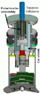
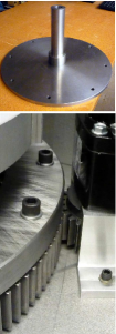
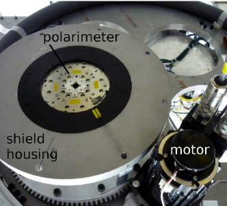
Figure 5: Active/passive shield, rotation design, and InFOC$\mu$S X-ray telescope. Left: X-Calibur polarimeter, embedded by the CsI active shield, as well as the electronic readout and azimuthal rotation bearing. 2^nd from left, top: Tungsten cap with collimator, only allowing X-rays from the mirror to enter the shield. 2^nd from left, bottom: Motor and ring bearing to rotate polarimeter/shield assembly. 2^nd from right: Opened pressure vessel with shield/X-Calibur installed (tungsten cap removed). The X-ray beam enters the polarimeter through the hole in the top plate. Right: The InFOC$\mu$S balloon gondola/truss with active pointing control and the X-ray mirror installed. The pressure vessel is installed in the back.

3.4 The Shield

During the balloon flight, the polarimeter will be hit by charged and neutral particle backgrounds with different spectral signatures and intensities. These backgrounds reduce the signal-to-noise ratio and, in the case of non-isotropic fluxes, can even lead to a fake polarization signature. In order to suppress these backgrounds, the polarimeter and the front-end readout electronics are operated inside an active CsI(Na) anti-coincidence shield. The $2.7\,\rm{cm}$ thick CsI crystal of the shield covers the sides and the bottom of the polarimeter and produces scintillation light when particles interact. The top is protected by a passive tungsten plate/collimator (Fig. 5, left), blocking X-rays and particles that do not come from the X-ray mirror. The (active) CsI scintillator of the shield is read out by four Hamamtsu PMTs R 6233 which are biased at $V_{\rm{bi}}=+800\,\rm{V}$. The analog signal of all four PMTs is merged and in turn digitized. A programmable, digital discriminator decides on whether a shield flag $f_{\rm{shld}}$ is set on the CZT readout board (kept up for $6\,\mu\rm{s}$) and is merged into the data stream. The values of the discriminator and the width of the flag were optimized using a radio-active source to maximize the shield efficiency and minimize chance coincidences (see Sec. 7.1).

In order to reduce the systematic uncertainties of the polarization measurements, the polarimeter and the active shield will be rotated around the optical axis with $\sim 2\,\rm{rpm}$ using a ring bearing (see Fig. 5). The angle between the polarimeter/shield and the mounting fixture is read out by a code wheel with the accuracy of $1^{\circ}$. A counter-rotating mass can be used to cancel the net angular momentum of the rotating polarimeter assembly during the balloon flight. The computer reading the PMT and CZT events is part of the rotating assembly, and referred to as polarimeter CPU.

3.5 The InFOC$\mu$S X-ray Telescope

The X-Calibur polarimeter will be flown in a pressurized vessel located in the focal plane of the InFOC$\mu$S X-ray telescope Ogasaka et al. [2005]. The telescope is shown in the right panel of Fig. 5. A Wolter grazing incidence mirror focuses the X-rays onto the polarimeter. The X-Calibur scintillator rod will be aligned with the optical axis of the InFOC$\mu$S X-ray telescope (see Sec. 8.2). The focal length of the mirror is $8\,\rm{m}$ and the field of view is $\rm{FWHM}=10\,\rm{arcmin}$. The telescope truss of InFOC$\mu$S is only coupled to the gondola by a ball joint in a support cup with floating oil, allowing for full inertial pointing of the telescope with an accuracy of $7^{\prime\prime}$ and $15^{\prime\prime}$ RMS in altitude and azimuth, respectively. To maintain the decoupling between truss and gondola, any communication between the two systems is done by wireless connections. In addition to the rotating polarimeter CPU (see above), a second CPU as part of the X-Calibur subsystem (motor CPU) is installed in the pressure vessel (non-rotating) and controls the motors, and a temperature system. Power and data communication between the polarimeter CPU and the motor CPU is achieved by a Mercotac^® 830-SS rotating ring of mercury sliding contacts. Communication between the pressure vessel and the telescope gondola will be done via a wireless network. The data will be stored on solid state drives and will in parallel be down-linked to the ground.

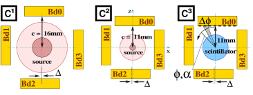
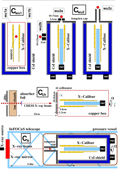
Figure 6: Different X-Calibur configurations referred to via $C_{\rm{env}}^{\rm{stp}}$. Top row: CZT detector geometries (see Fig. 3, left) viewed along the optical axis looking into the X-Ray beam. Each detector is tangentially translated by $\Delta=1\,\rm{mm}$. $C^{1}$: CZT detector cathodes being $c=16\,\rm{mm}$ away from the optical axis (regular-sized sealed radioactive source fits in between). $C^{2}$: Reduced distance of $c=11\,\rm{mm}$ (only compact sources). $C^{3}$: same as $C^{2}$ but with the scintillator rod installed. The definitions of $\Phi$ and $\Delta\Phi$ as used in Sec. 7 are illustrated. Bottom: Schematic sketches (not to scale) of X-Calibur installed in the different environments. $C_{\rm{wu}}$: Washington University; detector calibration in copper box ($C_{\rm{wu1a}}$) or in passive CsI shield ($C_{\rm{wu1b}}$); performance measurements in the active shield with different source positions ($C_{\rm{wu2a}}$, $C_{\rm{wu2b}}$, and $C_{\rm{wu2c}}$). $C_{\rm{ch}}$: X-Calibur/CHESS setup in hutch C1. The beam intensity is reduced by absorption foils; platinum ($C_{\rm{ch1}}$), or platinum and lead ($C_{\rm{ch3}}$). The X-Calibur polarimeter can be rotated around its optical axis (angle $\alpha$) which is aligned with the CHESS beam. $C_{\rm{ft}}$: X-Calibur installed in the InFOC$\mu$S X-ray telescope during a flight preparation campaign in Ft. Sumner.

3.6 X-Calibur Configurations and Data Sets

In order to characterize the different components and aspects of the X-Calibur polarimeter, different types of measurements were performed with different geometrical configurations of the instrument (e.g. with and without the shield, measurements without the scattering rod to calibrate the CZT detector response itself, illumination of the instrument with different X-ray sources from different angles, etc.). The measurements were performed at different facilities/locations (which we refer to as environments). The energy calibration and characterization of the CZT detectors was performed in the laboratory at Washington University (Sec. 6). Measurements of a polarized X-ray beam to study the performance of the polarimeter were conducted at the CHESS synchrotron facility at Cornell University (Sec. 8.1). Data were also taken with the fully integrated X-Calibur/InFOC$\mu$S telescope in a field campaign in Ft.Sumner, NM (Sec. 8.2). Measurements of the background (Sec. 7.1) were performed at Washington University, CHESS, and in Ft.Sumner. Throughout the paper, each configuration and location is referred to as $C_{\rm{env}}^{\rm{stp}}$ (‘env’ referring to the environment/location and ‘stp’ referring to the experimental setup). These different configurations are shown in Fig. 6 and will be referred to in the sections to follow in which the corresponding results are presented.

It should be noted, that some of the data presented in this paper were taken without the CsI shield (e.g. the data taken at the CHESS facility), not allowing one to use the shield veto for background suppression. Since separate background runs were taken and subtracted from the data, and the majority of measurements is signal-dominated, this does not affect any result or conclusion presented in this paper.

4 Reconstruction of Polarization Properties

The events recorded by X-Calibur consist of the digitized pulse height of one (or more) detector pixel(s), a time stamp, and flags describing whether the shield and/or the scintillator triggered. These raw events are first transformed into measured energies using the detector calibration. The reconstructed events are further processes in order to derive energy spectra and the polarization properties of the measured X-ray beam. This section outlines the corresponding procedures.

4.1 Definitions

The modulation in the measured azimuthal scattering distribution is the defining signature from which the polarization properties are derived. The modulation factor $\mu$ describes the polarimeter response to a polarized beam and is used to reconstruct the polarization properties. Assuming a $100\%$ linearly polarized X-ray beam, the minimum ($C_{\rm{min}}$) and maximum ($C_{\rm{max}}$) number of counts of the azimuthal scattering distribution define:

$$\mu=\frac{C_{\rm{max}}-C_{\rm{min}}}{C_{\rm{max}}+C_{\rm{min}}}.$$ (3)

It represents the modulation amplitude of a $100\%$ polarized beam and depends on the polarimeter design and the physics of Compton-scattering.

The performance of a polarimeter can be characterized by the minimum detectable polarization (MDP) as the minimum fraction of polarization that can be detected at the $99\%$ confidence level for a given time of observation $T$. Assuming a polarimeter that detects all Compton-scattered photons with an ideal angular resolution – in this case $\mu$ becomes the modulation amplitude averaged over all solid angles and the Klein-Nishina cross section – one can estimate the MDP by integrating the scattering probability distribution Weisskopf et al. [2011]; Kislat et al. [2015b] ($R_{\rm{src}}$ and $R_{\rm{bg}}$ are the source and background count rates, respectively):

$$\rm{MDP}\simeq\frac{4.29}{\mu R_{\rm{src}}}\sqrt{\frac{R_{\rm{src}}+R_{\rm{bg}}}{T}}.$$ (4)

4.2 X-Calibur Event Reconstruction and Selection

Each recorded X-Calibur event contains an event number, a GPS time stamp $T_{\rm{gps}}$, the orientation angle $\theta_{\rm{w}}$ of the shield/polarimeter with respect to the mounting plate (read by a code wheel), and a list of CZT detector pixels that were hit (up to nine) including their digitized pulse heights. Furthermore, two flags are merged into the data stream: (i) a flag $f_{\rm{shld}}$ that indicates whether the PMTs reading the active CsI shield got a signal exceeding the defined discriminator threshold, and (ii) a flag $f_{\rm{sci}}$ that indicates if the PMT reading the central scintillator rod of the polarimeter (see Fig. 3, left) exceeded its discriminator threshold. The average analog rise/fall times $\tau_{\rm{r}}$/$\tau_{\rm{f}}$ (time for a signal rise from $10-90\%$ of the amplitude) of the folded scintillator/PMT response were measured for the shield and for the scintillator. For the shield we find $\tau_{\rm{r}}^{\rm{shld}}\approx 70\,\rm{ns}$ and $\tau_{\rm{f}}^{\rm{shld}}\approx 2.6\,\mu\rm{s}$, respectively. The response of the scintillator rod of the polarimeter is much faster: $\tau_{\rm{r}}^{\rm{sci}}\approx 3.0\pm 1.3\,\rm{ns}$ and $\tau_{\rm{f}}^{\rm{sci}}\approx 13.7\pm 5.1\,\rm{ns}$ for cosmic rays, and $\tau_{\rm{r}}^{\rm{sci}}\approx 4.7\pm 2.7\,\rm{ns}$ and $\tau_{\rm{f}}^{\rm{sci}}\approx 13.5\pm 5.0\,\rm{ns}$ for a Cs¹³⁷ source placed at configuration $C_{\rm{wu2c}}^{3}$, respectively. Upon a CZT trigger, the event readout is delayed by $2.5-3.3\,\mu\rm{s}$ (jitter) to allow the shield and scintillator PMT signals to built-up and being converted into the corresponding flags. The flags $f_{\rm{shld}}$ and $f_{\rm{sci}}$ are kept up for a duration of $6\,\mu\rm{s}$.

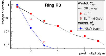
Figure 7: Distribution of pixel multiplicities $m$ for events taken with different sources (recorded in detector ring R3): Cosmic ray (CR) background in the laboratory, energy calibration using Eu¹⁵², Eu¹⁵² calibration restricting event energies to $E<80\,\rm{keV}$, and data taken at the $40\,\rm{keV}$ CHESS beam (see Sec. 8.1).

For each event, the pulse heights of all contributing channels/pixels $i=1...m$ are transformed into energies $E_{i}$ using the channel calibration, see Eq. (13) in Sec. 6.1. The total energy of the CZT event is $E=\sum_{i}E_{i}$. The number of pixels $m$ participating in the event is referred to as the pixel multiplicity. Selection cuts can be applied to the data based on the event properties mentioned above: $T_{\rm{gps}}$, $\theta_{\rm{w}}$, $E$, $m$, $f_{\rm{shld}}$, and $f_{\rm{sci}}$. Figure 7 shows the distribution of $m$ for different source types (measured in detector ring R3). It can be seen that sources with high energy contributions (such as the cosmic ray background or Eu¹⁵² with its $E>100\,\rm{keV}$ energy lines) have $m=1$ pixel event contributions of $\simeq 70\%$. Sources with energies concentrated in the $20-80\,\rm{keV}$ interval, relevant for X-Calibur, have $m=1$ contributions of $>90\%$ (e.g. the $40\,\rm{keV}$ CHESS beam, see Sec. 8.1). This is explained by the fact that low energy X-rays deposit smaller and more concentrated charge clouds in the CZT with a reduced chance of charge sharing between pixels (that would cause $m\geq 2$ events). Therefore, an event selection cut on $m=1$ is a reasonable way for background subtraction without loosing signal events at low energies. Cuts on the energy $E$ and the shield flag $f_{\rm{shld}}$ will further reduce the background (see Sec. 7.1). A selection cut on the scintillator flag $f_{\rm{sci}}$ selects a very clean sample of events that Compton-scattered in the scintillator. This has the potential to further reduce the background – however, with a loss in efficiency at low energies (see Sec. 7.2). However, a cut on $f_{\rm{sci}}$ is optional and not a requirement for sensitive polarization measurements with X-Calibur.

4.3 Energy Spectra

Energy spectra are used to study the scattering properties of the polarimeter and mark an intermediate step to derive the energy-dependent polarization properties. Energy spectra can be derived for individual pixels or for groups of pixels (e.g. a CZT detector or a detector ring R). The energy spectra shown in this paper are normalized to the acquisition time (dead time corrected), the anode detector surface covered by the corresponding pixel group and the width of the energy bins. Note, the limited dynamical range of the charge digitization of individual pixel channels will lead to discrete energies. Given the different energy calibrations of the channels, these will differ from pixel to pixel. This difference can lead to binning artifacts in energy spectra that are obtained from a small group of pixels.

4.4 Polarization Properties

The signature of a polarized beam will be imprinted in the azimuthal scattering distribution of recorded events (see for example Figs. 24 or 25 in Sec. 8.1). Either the scattering distribution itself, or a method involving the Stokes parameters, can be used to extract the polarization fraction $r$ and polarization direction $\Omega$. First, the details of the detector geometry have to be carefully considered in the analysis, as outlined below.

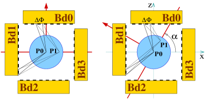
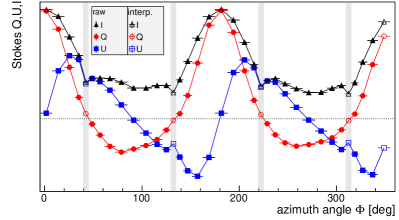
Figure 8: Left: Angular coverage of two selected CZT pixels within a single-pixel ring for different beam positions $P$. For a non-rotating detector (left) the angular coverage for each pixel only needs to be calculated once. In the rotating system (right) the beam offset in the horizon system (solid arrow) leads to varying angular coverage per pixel depending on the current rotation $\alpha$ that have to be updated on an event-by-event basis. Note, the pixel contacts are physically deposited on the backside of the detectors but are shown on the front side (facing the scintillator) for a better illustration of the angular measurement. The cyan dashed arrows indicate the $x/z$ detector coordinate system. Right: Stokes parameters $Q$, $U$, and $I$ as measured within a single-pixel ring for a polarized beam with $\Omega=90^{\circ}$. The pixels $j$ have varying angular coverage $\Delta\Phi_{j}$ (indicated by the horizontal error bars). The gray bands indicate the gaps between detector boards (see left panel). The filled data points show the measured values. The open data points show the interpolated Stokes parameters to recover the contributions missed by the gaps. Note, the entries in the figure are normalized to the solid angle $\Delta\Phi$ covered by each pixel. Therefore, the normalization leads to apparent jumps from the pixels to the values shown for the gaps. The open symbol at $\Phi\simeq 360^{\circ}$ corresponds to a dead pixel.

Azimuthal pixel coverage. The $360^{\circ}$ range in azimuth is covered by the $4\times 8=32$ pixels per single-pixel ring (see Fig. 8, left). Different pixels cover different azimuthal ranges $\Delta\Phi$ with respect to the center of the scattering rod which defines the optical axis. Therefore, the four sides of detector boards lead to a 4-fold symmetry in the scattering distribution (Fig. 24). This purely geometrical effect can be corrected for by dividing the counts $C_{j}$ in each pixel $j$ by its azimuthal coverage $\Delta\Phi_{j}$.

Azimuthal pixel coverage for beam offsets. A special situation arises if the optical axis of the X-ray beam is not aligned with the geometrical axis of the polarimeter (see $P_{1}$ in Fig. 8, left). Such an offset, if not corrected, will introduce asymmetries in the azimuthal scattering distributions and can mimic a wrong polarization signature (see Sec. 8.3 for a detailed study). Assuming a known offset vector $\vec{P}1$, the azimuthal coverage $\Delta\Phi_{p1,j}$ can be recalculated for each pixel $j$. This correction re-aligns the origin of the detector system with the beam axis and strongly reduces the systematic effect introduced by the offset. In the case of sufficient event statistics, first moments can be used to estimate the beam offset from the data itself (see Sec. 8.3). If the polarimeter is rotating, the beam offset in the horizon system will rotate in the detector system (see Fig. 8, left). In this case $\Delta\Phi_{p1,j}$ has to be updated on an event-by-event basis, taking into account the current polarimeter orientation $\alpha$ measured by the code wheel.

Pixel acceptance and flat fielding. Individual pixels have different trigger efficiencies, energy thresholds and energy resolutions affecting the number of counts derived from a given energy interval. To correct for these differences, the pixels are flat fielded using Compton-scattered events recorded from a non-polarized X-ray beam that results in a flat azimuthal scattering distribution. For a single-pixel ring the event counts per azimuthal coverage $C_{j}/\Delta\Phi_{j}$ are averaged for all $j=1...32$ pixels and are used to determine a relative azimuthal acceptance $a_{j}$:

$$w_{j}=\frac{1}{a_{j}}=\frac{\Delta\Phi_{j}}{C_{j}}\frac{1}{N}\sum_{i=1}^{N}\frac{C_{i}}{\Delta\Phi_{i}}.$$ (5)

The pixel acceptance $a_{j}$ can in turn be used to weight individual events with $w_{j}=1/a_{j}$. Implicitly, $a_{j}$ depends on the event selection cuts – so that it has to be computed for the particular set of cuts applied to the data. Dead pixels cannot be recovered by a corresponding weight since they contribute zero events. However, once the polarimeter/shield assembly is rotating with respect to the polarization plane, the pixel acceptances can be ignored since they average out throughout the measurement – this includes the treatment of dead pixels.

Polarization properties derived from the azimuthal scattering distribution. Integrating $C_{j}/\Delta\Phi_{j}$ for each pixel $j$ in a certain energy range and weighting the individual counts with $w_{j}$ will result in the azimuthal scattering distribution. Here, the angular coverage $\Delta\Phi_{j}$ determines the horizontal error bar of the data point. The scattering distribution can be derived for individual detector rings. Fitting a sinusoidal function to the distribution (e.g. left panel in Fig. 24, Sec. 8.1) allows one to reconstruct (i) the orientation of the polarization plane (minimum), as well as (ii) the modulation of the data $\mu_{\rm{data}}$ following Eq. (3). The corresponding modulation factor $\mu_{\rm{sim}}$ is derived from simulations of a $100\%$ polarized beam (see Sec. 5) that are analyzed using the same set of event selection cuts. The polarization fraction $r$ of the measured beam is in turn calculated to be:

$$r=\frac{\mu_{\rm{data}}}{\mu_{\rm{sim}}}.$$ (6)

The effect of dead detector pixels and gaps between the detector boards (see Fig. 8, left) is accounted for automatically, since the corresponding points do not show up in the distribution and will not affect the fit.

Polarization properties derived from Stokes parameters. An alternative approach to reconstruct the polarization properties is based on the Stokes parameters Chandrasekhar [1960]; Kislat et al. [2015b] that are calculated for each event $k$:

$$q_{k}=\cos(2\Phi_{k}),\quad u_{k}=\sin(2\Phi_{k}),\quad i_{k}=1.$$ (7)

The Stokes parameters can be summed for a subset of the data consisting of $N$ events (e.g. over a specific energy interval and detector ring):

$$Q=\sum_{k=1}^{N}w_{j(k)}q_{k},\quad U=\sum_{k=1}^{N}w_{j(k)}u_{k},\quad I=\sum_{k=1}^{N}w_{j(k)}.$$ (8)

Here, each event $k$ (originating from pixel $j$) is weighted with $w_{j(k)}=1/a_{j(k)}$. Since each pixel $j$ covers a range in azimuth $\Delta\Phi_{j}=\Phi_{j,\rm{max}}-\Phi_{j,\rm{min}}$, the values $q_{k}$ and $u_{k}$ derived from the mean angle $\Phi_{j(k)}$ in a non-rotating system may lead to inaccurate and/or biased results. Therefore, the mean Stokes parameters $\left<q\right>_{j(k)}$ and $\left<u\right>_{j(k)}$ are calculated based on the covered range in azimuth of the corresponding pixel $j$:

$$\begin{split}\left<q\right>_{j(k)}&=\frac{1}{\Delta\Phi_{j(k)}}\int_{\Phi_{j(k),\rm{min}}}^{\Phi_{j(k),\rm{max}}}\cos(2\Phi)\,\rm{d}\Phi,\\ \left<u\right>_{j(k)}&=\frac{1}{\Delta\Phi_{j(k)}}\int_{\Phi_{j(k),\rm{min}}}^{\Phi_{j(k),\rm{max}}}\sin(2\Phi)\,\rm{d}\Phi.\end{split}$$ (9)

The values of $\left<q\right>_{j(k)}$ and $\left<u\right>_{j(k)}$ are in turn used in Eq. (8). The proper treatment of dead pixels and gaps between the detector boards Bd0-Bd3 (see Fig. 8, left) is crucial when working with the Stokes parameters in a non-rotating coordinate system, since a lack of events from a particular azimuthal direction $\tilde{\Phi}$ will lead to an increase/decrease in $\sum_{k}\left<q\right>_{j(k)}$ and/or $\sum_{k}\left<u\right>_{j(k)}$, systematically affecting the reconstructed polarization properties (see Fig. 8, right). The amplitude and sign of the resulting effect depends on the orientation between the polarization plane and the detector plane (assuming the gaps are located at angles of $45^{\circ}$, $135^{\circ}$, $225^{\circ}$, and $315^{\circ}$, see Fig. 8, left). If the planes are exactly parallel or exactly perpendicular, the effect leads to a maximal underestimation of $r$. An angle of $45^{\circ}$ (polarization plane being aligned with two of the four gaps) leads to the maximal overestimation of $r$. At angles of $45/2=27.5^{\circ}$ (and multiples thereof) the effect of detector gaps cancels. A simulation for the X-Calibur detector layout was performed and resulted in a systematic effect of $\pm 6\%$ for a $100\%$ polarized beam. Therefore, a correction has to be applied: (i) the $m=1,2,...$ azimuthal ranges $\delta\tilde{\Phi}_{m}$ covered by the gaps have to be identified in which the detector is not sensitive (ii) The distributions of $\delta Q/\delta\Phi$, $\delta U/\delta\Phi$, and $\delta I/\delta\Phi$ have to be collected as a function of $\Phi$ (Fig. 8, right). (iii) These distributions are in turn used to interpolate the data gaps $\delta\tilde{\Phi}_{m}$ from neighboring pixel to recover the ‘missing’ contributions in Eq. (8):

$$\begin{split}Q&\rightarrow Q+\sum_{m}\Delta\tilde{Q}_{m}\delta\tilde{\Phi}_{m},\\ U&\rightarrow U+\sum_{m}\Delta\tilde{U}_{m}\delta\tilde{\Phi}_{m},\\ I&\rightarrow I+\sum_{m}\Delta\tilde{I}_{m}\delta\tilde{\Phi}_{m}.\end{split}$$ (10)

The errors on the added sums are calculated using error propagation during the interpolation. Given the scalar nature of the Stokes analysis, there is no simple way of representing the azimuthal modulation of the scattering distribution. Therefore, it is useful to compare the Stokes results with the results obtained from the azimuthal scattering distribution (previous paragraph) in order to identify possible systematic effects. Note again, that a rotating polarimeter will not require a correction for dead pixels or detector gaps.

The Stokes sums in (8) or (10) can be used to reconstruct the polarization fraction $r$ and polarization angle $\Omega$:

$$\begin{split}r&=\frac{2}{\mu_{\rm{sim}}}\frac{\sqrt{Q^{2}+U^{2}}}{I},\\ \Omega&=\frac{1}{2}\rm{atan}(U/Q).\end{split}$$ (11)

Results from $l$ independent measurements (e.g. from different detector rings) can be combined in a weighted average. Since the polarization fraction is always positive it can lead to an overestimation if the true polarization fraction is in the MDP regime of the data set, see Eq. (4), where the error bars are highly asymmetric. This systematic effect can be avoided by averaging a set of modified Stokes parameters:

$$\begin{split}Q^{\prime}&=\sum_{l}\frac{2w_{l}}{\mu_{\rm{sim,l}}}\frac{Q_{l}}{I_{l}},\quad U^{\prime}=\sum_{l}\frac{2w_{l}}{\mu_{\rm{sim,l}}}\frac{U_{l}}{I_{l}},\\ r^{\prime}&=\frac{1}{L^{\prime}}\sqrt{Q^{\prime 2}+U^{\prime 2}}\quad{\rm with}\quad L^{\prime}=\sum_{l}w_{l}.\end{split}$$ (12)

The weights $w_{l}=1/\sigma_{l}^{2}$ account for the statistical uncertainties of the individual measurements $l$.

Unfolding analysis. An unfolding analysis that takes into account the energy-dependent detector response and photon detection efficiencies and that can be used to reconstruct polarization fraction and angle as a function of true photon energy will be described in a separate paper Kislat et al. [2015a].

Forward folding. Recording the azimuthal scattering distributions with planar detectors will lead to projection effects that depend on the polar angle of the scattering in the scintillator. For most parts of the polarimeter these effects are negligible, since (i) a particular detector ring sees the superposition of different polar scattering angles canceling the effect, and (ii) the same effect is present in the simulations that are used to determine the polarization fraction following Eq. (6). Only for polarization fractions $r\ll 1$ measured in detector ring R1, which sees only back-scatter events, a second order correction may be needed. To fully take into account these effects, the data can be analyzed with a forward folding method (which is beyond the scope of this paper). The modeling of the pixel acceptance in R1, only affecting measurements with the non-rotating polarimeter, will also be slightly affected by the effect.

5 Simulations

Simulations of the energy-dependent response of the X-Calibur polarimeter are needed in order to reconstruct the polarization properties from measured data (see Sec. 4.4). The detector geometry is modeled and the X-ray flux/spectrum was simulated for the different experimental setups in which the data presented in this paper were taken. The simulations were performed in the following steps.

1. Physics interactions, scatterings, and energy depositions in the scintillator and the CZT detectors were simulated using GEANT4 with the Livermore low-energy electromagnetic model list.

2. The charge collection efficiency as a function of depth-of-interaction in the CZT detectors was determined using an in-house developed software to (i) calculate the 2D electric potential inside the detector crystals followed by (ii) the integration of the weighting potential Jung et al. [2007] along the charge transport tracks, resulting in the collected charge for each energy deposition (using a dielectric constant for CZT of $10$). The simulations are valid for detectors with strip anode contacts but will roughly resemble the response for pixelated detectors, as well. A mobility of electrons/holes of $\mu_{\rm{e}}=1000\,\rm{cm}^{2}/\rm{V}/\rm{s}$, and $\mu_{\rm{h}}=-120\,\rm{cm}^{2}/\rm{V}/\rm{s}$ is assumed, as well as life times of $\tau_{\rm{e}}=10^{-6}\,\rm{s}$ and $\tau_{\rm{h}}=4\cdot 10^{-6}\,\rm{s}$, respectively. This corresponds to a mobility-lifetime product of $\mu_{\rm{e}}\tau_{\rm{e}}=10^{-3}$ which is in reasonable agreement with the values measured for a selection of the detectors used in X-Calibur (see Fig. 13, bottom).

3. The energy resolution (asymmetric Gaussian function, implicitly including the electronic readout noise) and energy threshold were measured from real data (Sec. 6.2) and were folded into the simulations on a pixel-by-pixel basis. However, differences in channel trigger efficiencies were not simulated. Using the reversed energy calibration in Eq. (13), the simulated events were in turn converted into the X-Calibur data format (ASIC/channel ID and digitized raw pulse height) and can be analyzed in the same way as the measured data.

4. Since we find that the simulations do not properly account for low energy tails in the detector response (see next paragraph), an empirical model was used to scatter an exponential tail $T(E)=A\cdot\exp(E/E_{\rm{t}})$ into the simulations with a relative fraction of $f=0.45$ per energy deposit. The parameter $E_{\rm{t}}=15\,\rm{keV}$ (at $E=40\,\rm{keV}$) and $E_{\rm{t}}=30\,\rm{keV}$ (at $E=120\,\rm{keV}$) was interpolated in $\log E$ for the energy range covered.

5. The scintillator trigger flag $f_{\rm{sci}}$ was generated for each event based on the scintillator trigger efficiency determined from real data (see Fig. 20 in Sec. 7.2).

Different scenarios/setups were simulated, reflecting the measurements and studies presented in this paper.

CZT detector response. To test the validity of the simulation chain, the direct illumination of a single CZT detector with a Eu¹⁵² point source was simulated – corresponding to the experimental setup used for the detector calibration measurements presented in Sec. 6.1. The comparison between the simulations and data (Fig. 10, right) shows reasonable agreement in terms of line positions, widths, and threshold effects. However, if ignoring step (4) of the simulation chain (‘Sim’ in the legend of Fig. 10), a lack in continuum emission can be seen in the simulations. This motivated the introduction of step (4) which leads to a reasonable agreement between data and simulations over the whole energy band relevant for X-Calibur (‘Sim+’ in the figure legend). Possible reasons for the continuum in the data may be related to details in the detector response or back-reflection of emitted X-rays from the source off the surrounding fixture that is not simulated. It should be noted that the goal of the CZT simulations is not to find an accurate model for the detector response – but rather a suited parameterization that reproduces the integral spectral response for the different energy bins.

CHESS beam. X-Calibur performance measurements were performed at the highly polarized synchrotron X-ray beam at the CHESS facility – providing a strong, mono-energetic X-ray beam (Sec. 8.1). A corresponding set of simulations was performed using steps (1)-(5), resembling the CHESS setup of pencil-beam X-rays (polarized and non-polarized) at $40\,\rm{keV}$, $80\,\rm{keV}$, and $120\,\rm{keV}$ entering the polarimeter along the optical axis of the scintillator. Detector pixels that were excluded during the CHESS data runs were also excluded in the simulations to resemble a configuration close to the one used for the measurements. The trigger efficiency of the scintillator as a function of energy deposition was derived from the CHESS data (see Fig. 20 in Sec. 7.2) and was fed into the simulations in step (5) to generate the trigger flag $f_{\rm{sci}}$ on an event-by-event basis. No backgrounds were simulated in the case of the CHESS measurements since the measurements were completely signal-dominated.

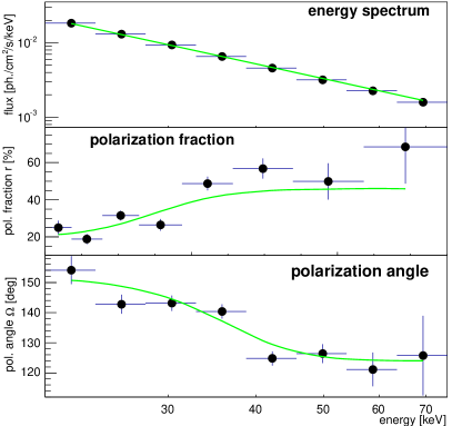
Figure 9: Simulated X-Calibur observations of the Crab nebula ($5.6\,\rm{h}$), taken from Guo et al. [2010]. The data points show the reconstructed flux (top), the fraction of polarization (middle), and polarization angle (bottom). The lines show the assumed flux, polarization fraction and polarization direction.

Balloon flight. A balloon flight in the focal plane of the InFOC$\mu$S mirror assembly was assumed in an earlier simulation Guo et al. [2010] that only involved step (1) in the above chain. The effective detection areas of the X-ray mirror are $95/60/40\,\rm{cm}^{2}$ at $20/30/40\,\rm{keV}$, respectively. We accounted for atmospheric absorption at a floating altitude of $130,000$ feet using the NIST XCOM attenuation coefficients and an atmospheric depth of $2.9\,\rm{g/cm}^{2}$ (observations performed at zenith); the atmospheric transmissivity rapidly increases from $0$ to $0.6$ in the $20-80\,\rm{keV}$ range. The trigger efficiency of the scintillator scatterer was assumed to be $f_{\rm{sci}}=1$ above an energy deposition of $2\,\rm{keV}$ and $f_{\rm{sci}}=0$ below.

We simulated the most important backgrounds such as the cosmic X-ray background Ajello et al. [2008], albedo photons and cosmic ray protons and electrons Mizuno et al. [2004]. The neutron background was not modeled since a detailed study of Parsons et al. [2004] showed that the contribution in CZT can be neglected. Different shield configurations and shield thicknesses were simulated. The configuration shown in Fig. 5 (left) represents an optimized compromise balancing the background rejection power and the mass/complexity of the shield. A Crab-like source was simulated for a $5.6\,\rm{hr}$ balloon flight. We assumed a power law energy spectrum, and a continuous change of the polarization fraction and angle between the values measured at $5.2\,\rm{keV}$ with OSO-8 Weisskopf et al. [1978] and at $E>100\,\rm{keV}$ with INTEGRAL Dean et al. [2008] by modeling a transition following a Fermi distribution.

For a Crab-like source the simulations predict an event rate of $1.1(3.2)\,\rm{Hz}$ with (without) requiring a triggered scintillator coincidence ($f_{\rm{sci}}=1$). Figure 9 compares the simulation results with the assumed model curves; the errors were computed in a similar way as described by Weisskopf et al. [2010]. Simulations performed at different zenith angles $\theta$ show that the source rate scales with $(\cos\theta)^{1.3}$ which is taken into account for simulating astrophysical observations. More details about these simulations are discussed in Guo et al. [2010] and Guo et al. [2013].

6 CZT Detector Characterization

The performance of the individual CZT detectors used in X-Calibur is coupled to the performance of the polarimeter as a whole – including its energy threshold and its energy resolution. This section describes the energy calibration of the individual CZT detectors (Sec. 6.1), as well as measurements of the energy threshold and energy resolution (Sec. 6.2). The CZT performance serves as important input for the simulations described in Sec. 5. In contrast to the laboratory, the polarimeter will be operated in an environment of varying temperature conditions during the balloon flight which motivates the study of the temperature dependence of the CZT detector performance which will be described in Sec. 6.3.

In order to quantify the characteristics of individual pixels, the emission lines in the calibrated energy spectra are fitted with a Gaussian function. The peak position is described by the mean $E_{\rm{p}}$. To account for the asymmetric shape of the peaks (see for example Fig. 10), the fitted function allows for asymmetric spectral continua levels ($c_{1}$, $c_{2}$) and asymmetric peak widths ($\sigma_{1}$, $\sigma_{2}$) for the $E<E_{\rm{p}}$ (1) and $E>E_{\rm{p}}$ (2) regimes, respectively. The fit parameters are used to characterize the measured peak. The energy resolution is calculated as the full width half maximum, $\Delta E=\rm{FWHM}=2\sqrt{2\ln 2}\cdot\frac{1}{2}(\sigma_{1}+\sigma_{2})$. The peak rate is determined by counting the events in the interval $\pm 2\,\rm{FWHM}$ centered around $E_{\rm{p}}$, normalized by the observation time.

A Eu¹⁵² source is used as calibration/test source in a variety of studies presented in this paper. Eu¹⁵² emits X-ray lines at $39.5\,\rm{keV}$ ($\rm{K}_{\alpha 2}$), $40.12\,\rm{keV}$ ($\rm{K}_{\alpha 1}$), $45.7\,\rm{keV}$, $122.78\,\rm{keV}$, $244.7\,\rm{keV}$, $344.28\,\rm{keV}$, and at higher energies. The line at $40.12\,\rm{keV}$ is the strongest in the low energy triplet; relative to the $40.12\,\rm{keV}$ line, the $39.5\,\rm{keV}$ line is emitted at $55\%$ intensity and the $45.5\,\rm{keV}$ line at $31\%$ intensity. The $40.12\,\rm{keV}$, used as low-energy performance marker, is therefore fitted jointly with the two close-by lines that are set at fixed distance $\Delta E$ and fixed intensity relative to the $40.12\,\rm{keV}$ peak (with the free fit parameter $\sigma$ being the same for all three lines since the energy resolution of a detector pixel is not expected to change within a few keV). Including the two neighboring lines avoids systematic shifts and artificial broadening of the fitted peak (see Fig. 10, left).

6.1 Energy Calibration

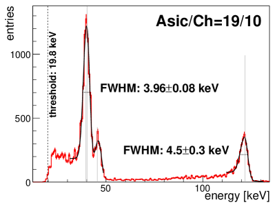
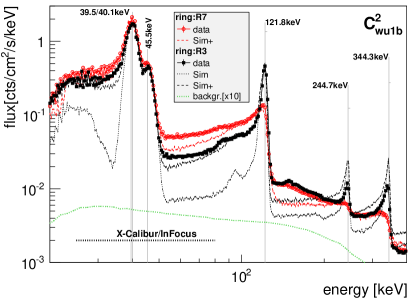
Figure 10: Eu¹⁵² energy spectra (direct CZT illumination). The vertical lines indicate the nominal X-ray line energies; relative heights indicate the emission intensity folded with the absorption probability in $5\,\rm{mm}$ CZT and $2\,\rm{mm}$ CZT (small tick), respectively. Data were taken with X-Calibur configuration $C_{\rm{wu1}}$ (see Fig. 6). Left: Spectrum of an individual detector pixel (linear energy axis, $C_{\rm{wu1a}}^{1}$). The dashed vertical line indicates the trigger energy threshold. The fitted functions ($40.1\,\rm{keV}$ and $121.8\,\rm{keV}$) are used to determine the peak position and energy resolution (FWHM). Right: Energy spectra summed over all pixels of the detectors in ring R3 ($5\,\rm{mm}$ thickness) and ring R7 ($2\,\rm{mm}$ thickness), respectively. Also shown are the simulated spectra with/without (Sim+/Sim) additional continuum (see Sec. 5). A CR background spectrum (scaled by a factor of $10$) is shown for reference. The horizontal dotted line indicates the energy range relevant for X-Calibur.

The energy calibration of the individual CZT detector pixels is done with a compact Eu¹⁵² source (cylindrical emitting volume with a diameter of $\simeq$$3\,\rm{mm}$) in the X-Calibur configuration $C_{\rm{wu1b}}^{2}$ in which the the scintillator rod is not installed (see Fig. 6). The source was successively placed at the centers of the detector rings – allowing to calibrate rings R1 to R8, one at a time. In a first step, an automatic routine is used to optimize the pixel trigger thresholds: data are taken in a special acquisition mode that adjusts ASIC/channel discriminators based on measured event rates for each pixel, such that the trigger threshold is as low as possible (maximizing the integral trigger rate), but at the same time is safely above the electronic noise regime. The noise regime leads to very high (artificial) trigger rates and differs from channel to channel. The routine works reliably for most channels. However, a visual inspection of all 2048 recorded energy spectra was performed to assure that channels with trigger thresholds set too high or too low (failed automatic detection of the noise regime) were adjusted manually.

About 5 million events were taken for each CZT detector (20 million events per ring R), and the known energy lines at $40.1\,\rm{keV}$ and $122\,\rm{keV}$ were used to determine the pedestal $p_{0}$ and amplification slope $a$ for each channel. The energy of a measured pulse height $p$ is in turn calculated using

$$E(p)=(p-p_{0})/a.$$ (13)

The left panel of Figure 10 shows the calibrated energy spectrum of a single pixel. The right panel shows the averaged calibration spectra of two chosen detector rings ($4\times 64$ pixels each). Also shown are the energy spectra obtained from the simulations of the corresponding setup (see Sec. 5). It can be seen, that the $2\,\rm{mm}$ detectors (ring R7) loose performance at energies $E>100\,\rm{keV}$, as compared to the detectors with $5\,\rm{mm}$ thickness (ring R3). However, in the $20-80\,\rm{keV}$ energy band, relevant for X-Calibur, both types of detector thickness perform at a similar level.

In addition to the temperature-dependence of the detector performance discussed in Sec. 6.3, another consideration has to be made when applying the calibration to the data. The CZT detectors used in X-Calibur are not setup for measuring the depth position of the X-ray interaction/absorption between the detector cathode and anode – referred to as the depth-of-interaction (DOI). The energy calibration in Eq. (13), however, depends on the average DOI of a given energy. The mean DOI, however, changes with the cosine of the inclination angle measured between the absorbed X-ray and the detector plane. The calibration was determined with the X-ray source located $c\simeq 11\,\rm{mm}$ above the center of the detector cathode (see Fig. 6, top). Depending on their geometrical locations, the pixels are hit under angles between $0-45^{\circ}$. X-rays Compton-scattering in the X-Calibur scintillator, on the other hand, can hit the CZT detectors at angles between $0-90^{\circ}$, which adds a systematic error/uncertainty to the reconstructed energy for small incident angles. However, in the $20-80\,\rm{keV}$ band the DOI distribution is very narrow and localized close to the cathode. Therefore, the angle dependence is negligible – the systematic shift of the reconstructed $40.1\,\rm{keV}$ line was experimentally constrained to be less than $1\%$ for shallow inclination angles.

A $<3\%$ fraction of ASIC channels were found to be dead, too noisy, or did not make contact to the detector pixel. These channels were excluded from the analysis and are marked with ‘x’ in the corresponding 2D plots shown in this paper (e.g. Fig. 11).

6.2 Energy Resolution and Threshold

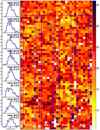
Figure 11: 2D distribution of energy thresholds of all X-Calibur pixels. In this representation, the four detector sides surrounding the scintillator (Bd0 to Bd3, see Fig. 3, left) are unfolded into a plane. The segments enclosed by dashed and dotted lines indicate the CZT detectors ($8\times 8$ pixels each). The elongated box (solid line in Bd0 to Bd3, each) indicates the position of the scintillator, even though it was not installed for this particular data set (configuration $C_{\rm{wu1b}}^{2}$, see Fig. 6, top). Pixels marked with ‘x’ were not included in the analysis. The left panels show the threshold distributions per detector ring R (the gray distribution shows the scaled average of all pixels).

To study the performance of the X-Calibur CZT detectors, the calibration data (Sec. 6.1) were used to characterize the energy spectra of individual pixels (see left panel of Fig. 10 for reference). The relevant properties studied in this section are the energy threshold, the fitted line/peak position, and the energy resolution (FWHM). As for the energy calibration, the data were taken with the configuration $C_{\rm{wu1b}}^{2}$ (see Fig. 6).

The energy threshold of a pixel is defined as the reconstructed energy $E_{\rm{thr}}$ above which the corresponding ASIC channel starts to trigger on events (see Fig. 10, left). The distribution of thresholds for all X-Calibur pixels is shown in Fig. 11. The thresholds vary from pixel to pixel, but no significant geometrical trends can be identified if comparing edge pixels versus central pixels, or pixels of detectors with different thickness ($5\,\rm{mm}$, rings R1-R5 versus $2\,\rm{mm}$, rings R6-R8). About $50\%$ of all pixels have an energy threshold of $E<20\,\rm{keV}$. It should be noted that one has to account for the energy resolution of a pixel in order to determine the analysis threshold that is about $3-4\,\rm{keV}$ higher. The thresholds shown in Fig. 11 reflect the status of the compact X-Calibur configuration. The thresholds of the detectors operated as a single unit are up to $5\,\rm{keV}$ lower (see Fig. 13).

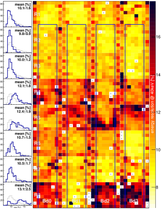
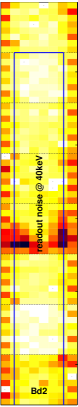
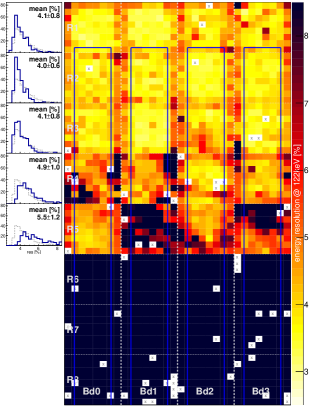
Figure 12: 2D distribution of the pixel-by-pixel energy resolution (compare with Fig. 11). Left: Energy resolution at $40.1\,\rm{keV}$. Middle: Electronic readout noise at $40\,\rm{keV}$ as determined using the ASICs internal test pulse generator (only shown for Bd2). The same range of the color scale as in the left panel is used. Right: Energy resolution at $121.8\,\rm{keV}$. This energy line is not well-defined in the energy spectra measured with the $2\,\rm{mm}$ detectors (see Fig. 10) so that results are only shown for the $5\,\rm{mm}$ rings R1 to R5.

Figure 12 shows the energy resolutions at $40.1\,\rm{keV}$ and $121.8\,\rm{keV}$, respectively. Detector rings R2 and R3 are the most sensitive ones when it comes to detecting the Compton-scattered X-rays in the polarization measurements (see Sec. 8.1). Therefore, the best performing $5\,\rm{mm}$ detectors were positioned in these rings accordingly. Some of the lower detector rings (R4 to R8) show regions with clearly poorer-than-average energy resolution. However, any asymmetry in azimuthal detector performance will cancel out due to the rotation of the polarimeter in the final mode of operation. The energy line at $121.8\,\rm{keV}$ is not well-defined in the spectra measured with the $2\,\rm{mm}$ detectors (see Fig. 10, right). Therefore, Fig. 12 only shows the $121.8\,\rm{keV}$ energy resolutions for the $5\,\rm{mm}$ detectors. The average energy resolution in rings R1 to R3 at $40.1\,\rm{keV}$ amounts to $4.0\,\rm{keV}$ ($10.0\%$); the corresponding value at $121.8\,\rm{keV}$ is $4.9\,\rm{keV}$ ($\simeq 4\%$). The average performance of rings R4 to R7 at $40.1\,\rm{keV}$ amounts to $4.6\,\rm{keV}$ ($\simeq 11\%$). The performance of the detectors in ring R8 is modest.

The energy resolution of a detector pixel is mainly determined by two factors – the quality of the CZT crystal and the noise of the read-out electronics. The electronic readout noise was determined for all channels using the ASICs internal pulse generator (see Sec. 3). The generator injects charge into the amplifier of the corresponding channel and allows one to test the trigger/digitization chain on a chennel-by-channel basis. 1000 events were taken per channel with the detectors connected and biased at nominal operation voltage (to also account for noise introduced by dark currents in the CZT). The results are shown in the middle panel of Fig. 12 for one of the four boards. More details on the electronic noise studies are presented in Sec. 6.3. Note, that the internal ASIC capacitor does not allow to inject charges that correspond to energies lower than $\approx 200\,\rm{keV}$. However, the noise versus energy trend seems to level off for energies lower than $\simeq 500\,\rm{keV}$ (see Fig. 15). Therefore, the absolute noise resolution measured at $\simeq 200\,\rm{keV}$ was used to estimate the relative noise contribution at $40\,\rm{keV}$, as shown in the middle panel of Fig. 12.

A comparison between the electronic noise and the energy resolution determined from the spectral lines shows that the low-energy resolution is dominated by the electronic noise. This kind of comparison can in general assist in localizing the cause for modestly performing detectors, e.g. by disentangling the contributions of electronic noise versus CZT crystal quality. The detector located in ring R5 of Bd2, for example, shows noisy regions in both, the Eu¹⁵² data, as well as in the electronic noise measurement – indicating a high leakage current as the reason for the sub-optimal performance. The ring R8 detector in the same board, on the other hand, does not exhibit a poorer energy resolution than others in terms of noise – therefore, the poor performance visible in the Eu¹⁵² data is probably related to a low CZT crystal quality.

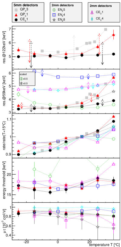
Figure 13: Temperature-dependent performance of individual CZT detectors. Each data point represents the average of $64$ pixels of a detector. Vertical arrows indicate the shift of the curve if considering only edge pixels of a detector (dashed direction), or only central pixels of a detector (solid direction). Top: Energy resolution at $122\,\rm{keV}$ (only shown for the $5\,\rm{mm}$ detectors). 2^nd from top: Energy resolution at $59\,\rm{keV}$. 3^rd from top: Peak detection rate of the $59\,\rm{keV}$ line normalized to the rate measured at $T=15^{\circ}\,\rm{C}$. 4^th from top: Energy threshold as determined after threshold optimization performed at the corresponding temperature. Bottom: Mobility-lifetime product $\mu_{\rm{e}}\tau_{\rm{e}}$ measured based on the $59\,\rm{keV}$ line.

On average, the side pixels of individual detectors exhibit a poorer than average energy resolution. At low energies, this shows up as a periodic structure on the left and right side of each detector. The same pattern can be seen in the electronic noise measurement (Fig. 12, left versus middle), and can therefore be attributed to the readout noise. This hypothesis is supported by the fact that the leads between the corresponding edge pixels and the ASIC channels are located on the ‘outside’ region of the printed circuit board – being more susceptible to noise pick up from the surrounding electronics. Subtracting the readout noise, these edge pixels do no longer show poorer energy resolution at low energies as compared to the other pixels. For energies $E>100\,\rm{keV}$ (not relevant for X-Calibur), the detector edge pixels show a reduced resolution in addition to the electronic noise component (‘frame-like’ structure surrounding each detector in Fig. 12, right). This is a known issue with CZT detectors and can be explained by a less homogeneous electric field in the edge regions of a detector, affecting the charge collection. The effect is less prominent (if visible at all) for the horizontal edge pixels, for which the field is stabilized by the neighboring detectors located in the same plane.

6.3 CZT Performance at different Temperatures

During a balloon flight the pressure vessel housing the polarimeter will undergo several changes in temperature that can potentially affect its performance. At float altitude, the vessel will be in an outside temperature environment of around $-20^{\circ}\rm{C}$. During daytime, the thermal radiation fields of the sun and the earth will provide additional sources of energy. During the night, the thermal radiation of the earth is the only external source of heat flow. The electronics inside the vessel generate heat at a rate of less than $100\,\rm{W}$. The outside of the vessel will be insulated using a layer of aluminized mylar (reflection of sun light and high emittance of thermal radiation) that will be contact-separated from the surface of the vessel with a layer of Dacron mesh. Furthermore, heater bands with a total power of $175\,\rm{W}$ are installed inside the vessel to guarantee a controllable temperature in the range of $0$ to $25^{\circ}\rm{C}$. This thermal design will prevent overheating during day-time and will avoid cold temperatures during the night. Nonetheless, variations in temperature of the polarimeter during flight are expected to some extent. Therefore, it is important to understand the temperature-dependent performance of the CZT detectors.

Individual CZT detectors were used to quantify the temperature dependence of the energy resolution, the energy threshold and the detection rate. Data were taken in a temperature chamber in the range of $T\in[-25;+35]^{\circ}\,\rm{C}$ with the detectors being illuminated with an Am²⁴¹ source ($59\,\rm{keV}$) and a Co⁵⁷ source ($122\,\rm{keV}$). The sources were located at a distance of $\simeq 2\,\rm{cm}$ above the detector cathode. The data were used to re-calibrate each detector (pixel-by-pixel) for each environment temperature in order to cancel temperature-dependent calibration effects. Since these measurements were time-intensive and could only be done for one detector at a time, the study was limited to a representative subset of the detectors shown in Tab. 1.

Temperature-dependent detector characteristics. The results of the measurements are shown in Fig. 13, averaged over all 64 pixels per detector. The $122\,\rm{keV}$ line is not well defined in the $2\,\rm{mm}$ detectors, so that the high-energy results are only shown for the $5\,\rm{mm}$ detectors. Given the limited sample of detectors, we cannot expect to attribute observed trends to a specific detector class (such as the brand); however, some general findings can be identified and are described in the following.

The energy resolution generally improves if reducing the temperature from $T=35^{\circ}\,\rm{C}$ to $T=0^{\circ}\,\rm{C}$. This effect is most prominent for the two tested Quikpak detectors and amounts to an improvement of up to $50\%$/$30\%$ at $59/122\,\rm{keV}$, respectively. The effect is much weaker for the Creative Electron detectors. For temperatures $T<0^{\circ}\,\rm{C}$, the resolution levels out. For some of the Endicott detectors ($2\,\rm{mm}$) it even gets poorer again; however, the two detectors showing this effect (EN₂4 and EN₂5) show very poor performance in general. All three $5\,\rm{mm}$ detectors show a much better energy resolution at $122\,\rm{keV}$ in the central pixels (indicated by the downward arrow in the top panel of Fig. 13) as compared to the edge pixels (upward arrow). Here, the aspect ratio allows for E-field lines to bulge out of the sides of the detector (see also Fig. 12). This difference is clearly less pronounces at $59\,\rm{keV}$ where the charge collection is much more concentrated in the cathode region of the detector crystal.

The peak detection rate at $59\,\rm{keV}$ (3^rd panel from the top in Fig. 13) shows a clear trend for all detectors: a reduced detection efficiency with decreasing temperature. This effect is not understood. Although the measurements were carefully set up, it cannot be excluded that a temperature-dependent contraction of the casing/fixture could have lead to a slight change in distance between the source and the detector as a function of environment temperature.

For each temperature, the energy thresholds were re-optimized. The results are shown in the 4^th panel of Fig. 13. No clear trends can be identified – the average energy threshold of the studied detectors lies between $15-20\,\rm{keV}$.

Measurements at different bias voltages $V_{\rm{bi}}$ were used to determine the mobility lifetime product $\mu_{\rm{e}}\tau_{\rm{e}}$. Data were taken at $V_{\rm{bi}}=-200\,\rm{V}$, $-500\,\rm{V}$, and $-700\,\rm{V}$ ($5\,\rm{mm}$ detectors) and at $V_{\rm{bi}}=-100\,\rm{V}$, $-150\,\rm{V}$, and $-200\,\rm{V}$ ($2\,\rm{mm}$ detectors), respectively. The shift of the line position with increasing $V_{\rm{bi}}$ was used to calculate $\mu_{\rm{e}}\tau_{\rm{e}}$ Lachish [2000]. The results are shown in the bottom panel of Fig. 13. No significant change in $\mu_{\rm{e}}\tau_{\rm{e}}$ can be identified for the temperature range studied. Jung et al. [2007] discuss the temperature dependence of Imarad High-Pressure Bridgman CZT detectors and find a decreasing trend of $\mu_{\rm{e}}\tau_{\rm{e}}$ for temperatures $T>10^{\circ}\,\rm{C}$ and for $T<-25^{\circ}\,\rm{C}$.

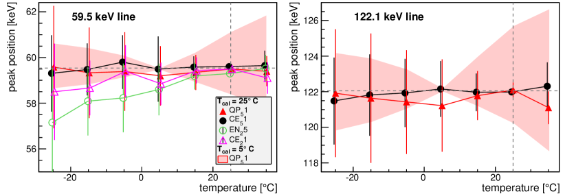
Figure 14: Reconstructed line energy for different temperatures using the calibration obtained at $T_{\rm{cal}}=25^{\circ}\,\rm{C}$ (dashed vertical line). The data points indicate the mean of the peak positions of all 64 pixels and the error bars represent the standard deviation of that distribution (separately derived for each temperature). The dashed horizontal line indicates the nominal line energy.

Temperature-stability of the calibration. In the studies shown in Fig. 13 all detector pixels were re-calibrated at each temperature. It is important to understand how the calibration itself changes with temperature. To study this effect, a reference calibration at $T_{\rm{cal}}=25^{\circ}\,\rm{C}$ was applied to the measurements taken at the different temperatures. The line positions at $59.5\,\rm{keV}$ and $122.1\,\rm{keV}$ were determined for the individual pixels. Each distribution (one per temperature) of reconstructed line positions was in turn characterized by its mean and its standard deviation. The results are illustrated in Fig. 14, where the standard deviation (spread of the corresponding distribution) is represented as error bar. For reference, the spectra of detector QP₅1 were corrected with the calibration obtained at $T_{\rm{cal}}=5^{\circ}\,\rm{C}$. While the mean reconstructed line energy does not change significantly, the widening of the error band indicates that individual channels show a temperature-dependent upward/downward drift of the line position. This makes it difficult to globally correct for temperature-dependent changes in the calibration – unless calibration data are taken for all 2048 X-Calibur channels at a variety of temperatures. The calibration changes by up to $\simeq 2\%$ for temperatures varying around $\pm 10^{\circ}\,\rm{C}$ relative to the reference calibration $T_{\rm{cal}}$.

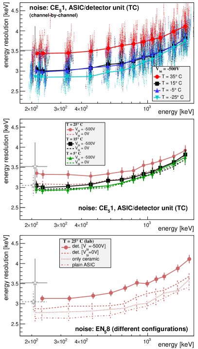
Figure 15: Electronic readout noise measured with the ASIC’s internal test pulser for different temperatures and different energies (detector CE₅1 and EN₅8). For reference, the gray asterisk marker indicates the 1 std.dev. range of all 2048 channels as operated in the X-Calibur assembly at room temperature of $T\approx 25^{\circ}\,\rm{C}$ with/without biased detectors (solid/dashed line). Top: Channel-by-channel noise (vertical dotted lines) and detector average with the detector being biased at $V_{\rm{bi}}=-500\,\rm{V}$. Middle: Detector averages for three different temperatures with and without the cathode bias $V_{\rm{bi}}$. Bottom: A series of $T\approx 25^{\circ}\,\rm{C}$ measurements with different configurations as described in the text.

Electronic noise. The read-out electronic contributes a certain amount of jitter to the measured energy resolution of a detector pixel. In order to quantify this contribution, a series of measurements was taken with detectors CE₅1 and EN₅8 (see Tab. 1) at different temperatures using the internal pulse generator of the ASIC (see Sec. 3). The detectors were operated in an electrically shielded copper box. With the detector being plugged into the ASIC, the measurements actually reflect the readout noise of the ASIC/detector assembly, rather than the noise of the ASIC alone. Different amounts of charge were injected (corresponding to different energies). The measured pulse heights were transformed to energies using the corresponding energy calibration determined for each temperature. For each configuration and channel, a total of 1000 events were injected. The calibrated distribution was fitted in order to determine the corresponding mean energy and energy resolution.

The results are shown in Fig. 15. At energies of around $200\,\rm{keV}$ the electronic noise of the ASIC/detector unit increases by $(21\pm 6)\%$ in the studied temperature range of $-25^{\circ}\,\rm{C}$ to $+35^{\circ}\,\rm{C}$. The shape of the energy-dependent noise curve depends on the temperature. At room temperature, the noise increases by $(20\pm 4)\%$ if going from $200\,\rm{keV}$ to $1.7\,\rm{MeV}$ and levels out around $3\,\rm{keV}$ at low energies. This suggests, that the energy resolution in the X-Calibur range ($\approx 4\,\rm{keV}$ at $40\,\rm{keV}$, see Fig. 12) is dominated by the electronic readout noise, rather than charge transport properties in the CZT crystal. The gray asterisk marker in Fig. 15 shows the 1 std.dev. range of the noise distribution of all 2048 data channels as measured at room temperature ($\approx 25^{\circ}\,\rm{C}$) in the final X-Calibur configuration, compare with Fig. 12 (middle).

The middle panel of Fig. 15 illustrates the effect of the bias voltage of the detector. A biased cathode at $T=25^{\circ}\,\rm{C}$ increases the low-energy noise by $(8\pm 5)\%$, whereas no noticeable change can be measured for temperatures lower than that. Therefore, the cathode bias only seems to systematically affect the readout noise for temperatures higher than $\simeq 15^{\circ}\,\rm{C}$.

The bottom panel in Fig. 15 shows the electronic noise measured at room temperature for different configurations: (i) the detector/ASIC unit with biased cathode, (ii) the detector/ASIC unit with unbiased cathode, (iii) the ASIC with a ceramic chip carrier but no detector bonded to it, and (iv) only the plain ASIC. It can be seen that steps (i)–(iii) each add $\approx 0.2\,\rm{keV}$ readout noise to the single-detector system. The average readout noise of the whole X-Calibur assembly (gray asterisk in Fig. 15) is shown for reference. Another series of measurements was performed with the plain ASIC at different temperatures (not shown). No significant noise trend could be identified in the $T=-20^{\circ}\,\rm{C}$ to $+25^{\circ}\,\rm{C}$ temperature range which leads to the conclusion that the temperature dependence of the readout noise of the ASIC/detector unit (top panel of Fig. 15) is mostly a result of the temperature dependence of the dark currents in the CZT crystal.

Caveats: The electronic readout noise varies from ASIC to ASIC and depends on the electronic shielding environment in which the ASIC is operated. Therefore, the comparison between the absolute noise levels of the single ASIC system shown in Fig. 15 and the average readout noise in the X-Calibur assembly should be treated with care; the relative noise trends found, however, can likely be applied to whole X-Calibur assembly. It should also be mentioned, that the cooling aggregates of the temperature chamber (increased activity at low temperatures) can potentially introduce external noise pick-up in the ASIC.

6.4 Summary of the Detector Calibration and Tests

Each detector pixel has been energy calibrated according to Eq. (13). With the current readout electronics and the compact X-Calibur configuration, the CZT detectors achieve a mean trigger threshold of $\simeq 21\,\rm{keV}$. The mean energy resolution at $40\,\rm{keV}$ in the three front-side detector rings R1-R3 (detecting most of the scattered events in the polarization measurements) is found to be $\Delta E_{\rm{czt}}\simeq 4\,\rm{keV}$ FWHM, when operated at room temperature. The energy resolution of the polarimeter as a whole is determined by the energy resolution of the individual detectors and by the energy deposited/lost in the scintillator ($\Delta E_{\rm{sci}}=0-5.4\,\rm{keV}$ at $40\,\rm{keV}$). The energy resolution of the detectors is thus not entirely negligible and X-Calibur would benefit from an optimized readout ASIC. We are currently working on modifying and adopting the HD-3 ASIC de Geronimo et al. [2003]; Vernon et al. [2010]. Using a pre-amplifier chain optimized for the $2-100\,\rm{keV}$ energy range, we expect a trigger threshold of $1.7\,\rm{keV}$ and electronic readout noise of $\simeq 550\,\rm{eV}$ RMS. The noise contribution of the new ASIC to the energy resolution of the polarimeter would be negligible for all energies above $20\,\rm{keV}$. The low energy threshold can potentially be used on a satellite-borne version of the polarimeter.

The effective energy threshold of the polarimeter is slightly higher than the energy threshold of the individual CZT detectors, as a $25\,\rm{keV}$ photon looses up to $2.2\,\rm{keV}$ in the scatterer. However, the polarimeter will detect a large fraction of the X-rays at 125,000 feet flight altitude, as the residual atmosphere only transmits photons above $\simeq 25\,\rm{keV}$.

Even though the temperature-dependent trends in energy resolution would favor operating the detectors at $T\leq 0^{\circ}\,\rm{C}$ (Fig. 13, top), the thermal design of the X-Calibur assembly and local internal heat built-up of the polarimeter during the balloon flight makes an operation at $T\simeq(15\pm 10)^{\circ}\,\rm{C}$ a more likely scenario – still guaranteeing a reasonable energy resolution for most of the detectors. A change in temperature, which will be monitored during flight, leads to a shift in reconstructed energy – which can go either way (Fig. 14). Ideally, one should use a data base of temperature-dependent calibration values on a pixel-by-pixel basis to correct for the temperature trends. If ignoring the temperature-dependence of the calibration, a systematic error on the reconstructed energy of a few percent has to be accounted for in the temperature interval of $\pm 10^{\circ}\,\rm{C}$ around the calibration temperature. For the first X-Calibur flight, we will choose the second option.

7 X-Calibur: Instrument Characterization

This section describes measurements of the fully assembled polarimeter installed in the CsI shield. The goal of the measurements is to characterize the efficiency of the shield, and to estimate the background levels in the different (ground-based) environments the polarimeter was operated in (Sec. 7.1). The reduction of the background is crucial in order to perform sensitive measurements of the polarization properties of astrophysical sources, see Eq. (4).

The X-rays that enter the polarimeter along the optical axis will produce a certain amount of scintillation light when scattering in the scintillator rod which is read out by a PMT. The efficiency curve, describing the trigger probability for different energy depositions in the scatterer, is discussed in Sec. 7.2. As will be shown in Sec. 7.1, a high trigger efficiency of the scintillator will allow a further reduction of the background. The efficiency curve is fed into the simulations that were discussed in Sec. 5. The measurements described in this chapter were done with disk-like radioactive sources with a diameter of $\simeq 0.5\,\rm{cm}$.

7.1 Shield Performance and Cosmic Ray Background

The shielding and suppression of backgrounds is a crucial task for sensitive polarimetry measurements. The background in the ground-based measurements presented in this paper (non-flight) results mostly from secondary particles produced in air showers in the earth’s atmosphere, induced by cosmic rays (CRs). The flux of the secondary particles depends on the geographical location at which the measurement is performed, and on the structure/materials of the building in which the polarimeter is operated (partly shielding the secondary particles). As can be seen in Fig. 7, the CR background has a higher fraction of multiplicity $m\geq 2$ pixel events as compared to Compton-scattered X-rays in the $E<100\,\rm{keV}$ regime, relevant for the X-Calibur polarimetry measurements. In general, the distribution of $m$ depends on the energy and the kind of interaction; high-energy muons (ionization), for example, trigger events along a row of pixels (unless they cross the detector perpendicular to the pixel plane). Low energy X-rays, on the other hand, are photo-absorbed with a charge deposition usually contained well within one pixel. Therefore, a requirement of $m=1$ pixel events already suppresses the background for the polarization measurements by a certain amount.

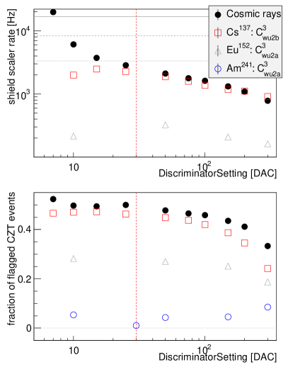
Figure 16: Optimization of the shield discriminator using three different data runs (a)-(c), as described in the text. The background contribution is subtracted for the runs with Cs¹³⁷ outside shield (b), and for Am²⁴¹/Eu¹⁵² on the optical axis (c). The dashed vertical line indicates the optimal discriminator setting. Top: Shield trigger rate for different threshold settings. The horizontal lines indicate the rates corresponding to $10/5/2\%$ (from top to bottom) dead time produced by the shield vetoes. The noise regime starts to dominate around DAC $<20$; this in turn leads to an underestimation of the Cs¹³⁷/Eu¹⁵² trigger contribution since the CR background is subtracted. In the case of the Am²⁴¹ source, no significant trigger rate above background was measured. Bottom: Fraction of detected CZT events that are vetoed with $f_{\rm{shld}}=1$.

Optimization of the shield trigger threshold. A particle crossing the active shield (see Fig. LABEL:fig:ActiveShieldAndTelescope,_left)_produces_scintillation_light_in_the_CsI_crystal._The_crystal_is_read_by_four_PMTs_which_signals_are_summed_and_digitized. A programmable discriminator decides whether the shield veto flag $f_{\rm{shld}}$ is activated ($f_{\rm{shld}}$ is kept active for $6\,\mu\rm{s}$ per trigger) and merged into the data stream. Events with the corresponding flag can in turn be filtered out in the data analysis. In order to optimize the shield trigger efficiency, a series of measurements was performed with different settings of the discriminator. The measurements comprise: (a) cosmic ray background only, (b) a collimated Cs¹³⁷ source aimed from outside the shield at the X-Calibur CZT detector assembly (configuration $C_{\rm{wu2b}}^{3}$ in Fig. 6), and (c) collimated Am²⁴¹/Eu¹⁵² sources placed on the optical axis of the polarimeter (configuration $C_{\rm{wu2a}}^{3}$) to simulate X-rays from the X-ray mirror entering the polarimeter without interaction in the shield. Two shield characteristics were measured: (i) the raw trigger rate of the shield, and (ii) the fraction of triggered CZT events with $f_{\rm{shld}}=1$. The results are shown in Fig. 16. Since the cosmic ray background was present in all three runs, the X-ray data runs (b) and (c) were corrected for the rates measured in run (a). The setting of the discriminator was optimized according to the following criteria.

1. The dead time produced by noise triggers should not exceed a few percent (horizontal lines in Fig. 16). The Am²⁴¹/Eu¹⁵² sources located on the optical axis (c) should result in CZT events with a $f_{\rm{shld}}=1$ contribution as low as possible (no signal suppression).

2. For the CR (a) and Cs¹³⁷ (b) runs, the fraction of CZT triggers with $f_{\rm{shld}}=1$ should be as high as possible, reflecting a high rejection power.

We determined an optimal shield discriminator setting of $\rm{DACQ}=30$ which is indicated by the vertical line in Fig. 16. Note, the fraction of Eu¹⁵² events with $f_{\rm{shld}}=1$ is around $25\%$, which is probably due to X-rays that Compton scatter and interact with the shield and CZT – a result of not having a well collimated X-ray beam entering the polarimeter in this measurement.

Data set	$\left<T_{5\,\rm{mm}}\right>$	$\left<T_{2\,\rm{mm}}\right>$
	[mHz]	[mHz]
CZT initial calibration (Washington Univ.): $C_{\rm{wu1a}}^{1}$
Eu152 illumination	$7100$	$6200$
Background	$59$	$35$
Scintillator characterization (Wash. Univ.): $C_{\rm{wu2a}}^{3}$
Eu152 on optical axis∗	$31$	$8.7$
Background in shield (active)	$9.9(5.4)$	$4.9(2.0)$
CHESS synchrotron beam (Cornell Univ.): $C_{\rm{ch}}^{3}$
$40\,\rm{keV}$ X-ray beam	$1100$	$300$
Background	$13$	$8.4$
X-Calibur/shield/InFocus (Ft. Sumner): $C_{\rm{ft}}^{3}$
X-ray source∗	$853$	$190$
Background in shield (active)	$8.5(3.9)$	$4.7(1.6)$
X-Calibur flight (simulations)
Crab∗	$1.25$	$0.3$

Table 2: Average event trigger rates per CZT detector pixel for $5\,\rm{mm}$ detectors $\left<T_{5\,\rm{mm}}\right>$ and for $2\,\rm{mm}$ detectors $\left<T_{2\,\rm{mm}}\right>$. Rates are shown for the different measurements/environments presented in this paper (see Fig. 6). No event selection cuts are applied. Rates marked with a ‘*’ are background subtracted. The corresponding background spectra for the different data sets are shown in Fig. 17.

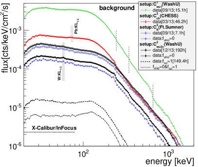
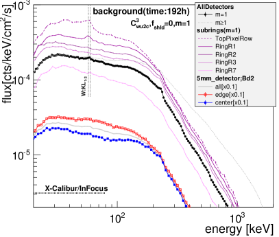
Figure 17: Cosmic ray background spectra (events with pixel multiplicity $m=1$, if not mentioned otherwise). The dotted vertical lines indicate the ranges of the $\rm{KL}_{1-3}$ transition energies of tungsten (W) and lead (Pb) which show up in some of the spectra. The X-Calibur/InFOC$\mu$S sensitive energy range is indicated, as well. Left: Spectra measured in different environments (see Fig. 6). Date and duration of the runs is given in square brackets. The (passive/active) CsI shield strongly reduces the background. The three dashed vertical lines on the $C_{\rm{wu1a}}^{1}$ spectrum represent the high-energy lines of Eu¹⁵² ($244.7\,\rm{keV}$ and $344.3\,\rm{keV}$) and Cs¹³⁷ ($661.7\,\rm{keV}$) for which an onset indication can be seen; the sources were stored in a lead bunker $\sim$$2\,\rm{m}$ away during the background measurements and were probably contributing to the spectrum at a low level. Right: Energy spectra for individual detector rings measured at Washington University in the active shield (after shield veto, $f_{\rm{shld}}=0$). We also show energy spectra (scaled by a factor of 0.1) from different pixels of the detectors on the readout board Bd2 to illustrate the difference between central pixels and pixels located on the edge of detectors, see also Fig. 18 for reference.

Cosmic ray background levels. Figure 17 shows the CR energy spectra ($m=1$ pixel multiplicity) measured in the CZT detectors at the different locations: the laboratory at Washington University ($C_{\rm{wu}}$), the CHESS X-ray beam facility ($C_{\rm{ch}}$, Sec. 8.1), and in Ft. Sumner ($C_{\rm{ft}}$, Sec. 8.2). For reference, the corresponding event trigger rates ($m\geq 1$) per pixel are summarized in Tab. 2. Note, that the actual pixel rates can vary quite substantial, since different pixels see different income fluxes depending on the type of measurement (e.g. an X-ray beam Compton scattered in the scintillator leads to a strongly depth-dependent illumination of CZT detectors, compare with Fig. 25). However, it can be seen that for most measurements presented in this paper the background can be neglected. During the balloon flight, however, the expected source-to-background ratio will be much lower and a proper understanding and the background suppression will be crucial Guo et al. [2010, 2013].

Even though the background at flight altitude will be different as compared to the ground-based CR background, some characteristics in the detector response can be discussed qualitatively based on the spectra shown in Fig. 17. While $\alpha$-particles interact close to the surface of the detector, muons as well as primary and secondary high-energy gamma rays will penetrate deeper and their energy deposition is proportional to the detector volume. This volume-dependent background rate can be seen by comparing the spectra (and trigger rates) measured with $5\,\rm{mm}$ versus $2\,\rm{mm}$ detectors. Note, that the spectra shown in Fig. 17 represent particle fluxes folded with the energy-dependent response of the CZT detectors (with an energy calibration derived from, and valid for, X-rays). The drop in event rate below $30\,\rm{keV}$, for example, is an effect of the superposition of the different trigger thresholds of the pixels contributing to the spectrum. The dynamical energy range covered by a single pixel saturates around $2000\,\rm{keV}$ (differing from pixel to pixel), so that the combined $m=1$ pixel spectra shown in Fig. 17 drop off around this energy. Allowing events with $m\geq 1$ multiplicities will extend the energy range (see Fig. 17, right) which is, however, not relevant for the operation of X-Calibur.

The CsI shield efficiency. Figure 18 shows the 2D distribution of event count rates from background data taken with X-Calibur installed in the CsI shield at Washington University. The rates are shown for two different energy bands. The left panels show the raw rates and the right panels show the rates after rejecting events that triggered the active shield, only allowing non-vetoed events ($f_{\rm{shld}}=0$). It again becomes obvious that the $5\,\rm{mm}$ detectors (R1-R5) collect more background compared to the $2\,\rm{mm}$ detectors (R6-R8). Furthermore, the edge pixels of the detector rows on the individual boards Bd0-Bd3 see a higher background rate as compared to central pixels (likely because of the higher exposed surface area detecting charged particles and low energy X-rays). The energy-resolved difference between edge and central pixels can be seen in Fig. 17, right ($5\,\rm{mm}$ detectors of boards Bd2): the central pixels show an almost two times lower background compared to edge pixels in the energy regime relevant for X-Calibur.

The background distribution after shield veto (Fig. 18, right) exhibits a spatial gradient with more background events being detected closer to the front side of the experiment, as that side is only shielded by the passive tungsten cap (see Fig. 5, left). In particular, the front-side (top) pixel row of ring R1, with its exposed detector side walls, suffers strongly from primary radiation leaking through the tungsten, as well as secondary particles being produced in the tungsten. Here, spectral signatures of the tungsten KL transitions can be identified in the measured spectra shown in Fig. 17 (right). Since this single pixel row is not crucial for the polarimetry sensitivity it can be excluded from the analysis.

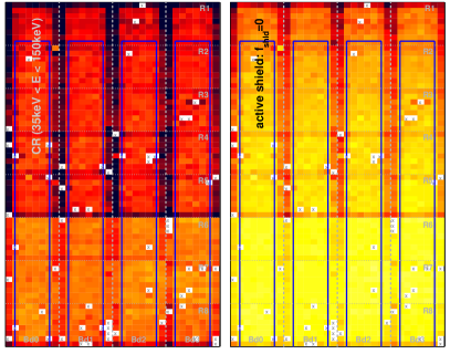
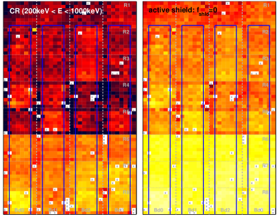
Figure 18: 2D maps of the CR count rates (pixel-by-pixel, representation same as in Fig. 11) of a $192\,\rm{h}$ background run with X-Calibur being installed in the active CsI shield ($C_{\rm{wu2c}}^{3}$ in Fig. 6). The tungsten cap is located at the top of each panel. The count rate is derived by integrating the corresponding energy spectra ($m=1$ events) in the given energy range: $35-150\,\rm{keV}$ (top) and $200-1000\,\rm{keV}$ (bottom). The left panel shows the measured rate (passive shield rejection only) and the right panel shows the non-vetoed events with $f_{\rm{shld}}=0$ (active and passive rejection). Left and right panels are shown with the same axis/color ranges, each.

The passive/active rejection efficiency of the CsI shield becomes obvious if comparing the different background spectra in Fig. 17, left. Moving the polarimeter from its copper housing (used in the initial test measurements, $C_{\rm{wu1}}^{1}$) into the CsI shield ($C_{\rm{wu2c}}^{3}$) reduces the background by roughly one order of magnitude due to passive shielding. Applying the $f_{\rm{shld}}=0$ veto from the active shield leads to an additional background rejection by a factor of $\sim$$2$. Note, that the recombination of the tungsten and lead $\rm{KL}_{1,2,3}$ transition energies (probably activated by CRs) can be identified in the background spectra. This feature is most prominent in the spectrum of ring R1 (Fig. 17, right) which is located closest to the tungsten cap.

It should be noted that an additional cut on the scintillator rod coincidence flag $f_{\rm{sci}}=1$ reduces the background by another $1.5$ orders of magnitude (Fig. 17, left) – strongly rejecting events that did not enter the polarimeter along the optical axis and interacted in the scintillator, see Sec. 7.2.

7.2 Compton-scattering and Scintillator Trigger Efficiency

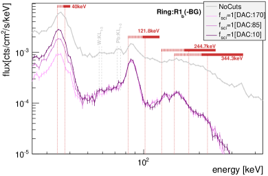
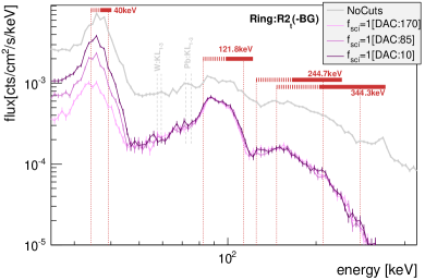
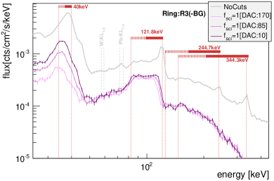
Figure 19: A lead-collimated Eu¹⁵² source enters the polarimeter along the optical axis and Compton-scatterers in the scintillator rod ($C_{\rm{wu2a}}^{3}$ in Fig. 6). The resulting CZT spectra ($m=1$, background subtracted) are shown for different rings. The horizontal lines indicate the complete range of possible energies $E_{\rm{czt}}$ after Compton-scattering (dotted: $180-90^{\circ}$, solid: $90-0^{\circ}$). The attached vertical dotted lines indicate the sub range for the particular ring – given its geometrical coverage of the scintillator. Spectra are measured with different scintillator trigger thresholds settings (Digital to Analog Converter, DAC) and are compared to the spectra without coincidence requirement (no cuts). The lead collimator prevents direct source hits (rings R1-R3), but scattered X-rays and/or activation of the $\rm{KL}_{1-3}$ transitions in tungsten (W) and lead (Pb) partly contaminate the spectra.

The central scintillator rod of the polarimeter (Fig. 3) acts as a Compton-scatterer for the incoming X-ray beam. At the same time, it produces scintillation light that is read out by a PMT. In order to characterize the Compton-scattering and the trigger response of the scintillator, a collimated Eu¹⁵² source was placed at the polarimeter entrance, illuminating the scintillator along the optical axis (see setup $C_{\rm{wu2a}}^{3}$ in Fig. 6). The Compton-scattered X-rays are recorded by the surrounding CZT detector rings. An X-ray enters the polarimeter with a certain energy $E_{\rm{line}}$, deposits the energy $\Delta E_{\rm{sci}}$ in the scintillator and is absorbed in a CZT detector with its post-scattering energy of $E_{\rm{czt}}=E_{\rm{line}}-\Delta E_{\rm{sci}}$. The amount of scintillation light can be assumed to be proportional to $\Delta E_{\rm{sci}}$.

Data were taken with different settings of the scintillator/PMT discriminator threshold (DAC). As can be seen in Tab. 2, the background level is not negligible in this measurement, so that background spectra without a X-ray source were recorded and subtracted. It should be noted, however, that X-rays scattered in the lead collimator and activation/recombination of the $\rm{KL}_{1,2,3}$ electron transitions in the lead collimator and the tungsten cap lead to a slight contamination of the measured spectra. These corresponding spectral features do not cancel out after CR background subtraction since they are (indirectly) introduced by the Eu¹⁵² source itself. Since those features will over-proportionally affect the data without the $f_{\rm{sci}}=1$ coincidence (X-ray paths that do not necessarily cross the scintillator), this may lead to an underestimation of the trigger efficiency (which in the ideal case would only compare Compton-scattered events in the scintillator with and without the $f_{\rm{sci}}=1$ trigger coincidence). The scintillator trigger efficiency for different energies $\Delta E_{\rm{sci}}$ is derived as follows.

Compton spectra. The resulting Compton-scattered energy spectra $E_{\rm{czt}}$ are shown in Fig. 19 for different CZT detector rings. Data are shown with and without the scintillator coincidence requirement. The energy $\Delta E_{\rm{sci}}$ deposited in the scintillator depends on the scattering kinematics, including the primary energy of the X-ray $E_{\rm{line}}$ and its scattering angle. The theoretical range of energies after $0-180^{\circ}$ Compton scattering is indicated by horizontal lines for the four main Eu¹⁵² energy lines. Due to geometrical reasons, some of the detector rings can only detect X-rays originating from a limited range of Compton-scattering angles. With the scintillator starting at ring R2 (Fig. 3, left), the sub rings R1_t, and R1_b, for example, can only detect back-scattered X-rays which deposit/loose the highest amount of energy $\Delta E_{\rm{sci}}$ in the scintillator – leading to a higher trigger probability. For a given incoming energy $E_{\rm{line}}$, the range of possible scattering angles translates into a range of possible Compton-scattered energies $E_{\rm{czt}}$. These ring-dependent sub ranges in scattered energy are indicated by the vertical lines in Fig. 19. Note, however, that the scattering angles/energies will not be equally distributed within these boundaries. One can qualitatively discuss the X-Calibur response to Compton-scattering for the different scattered energy lines.

$E_{\rm{line}}=40\,\rm{keV}$: The Compton-scattered energy range of the Eu¹⁵² line doublet ($39.52\,\rm{keV}$ and $40.12\,\rm{keV}$) only covers $E_{\rm{czt}}=34.2-40.1\,\rm{keV}$ at an energy resolution of $\Delta E_{40}\simeq 4\,\rm{keV}$. This makes it difficult to resolve structures in the scattered energy spectrum. However, the geometrical coverage of ring R1_b constraints the energy deposition in the scintillator to $\Delta E_{\rm{sci}}=2.4-5.4\,\rm{keV}$ since only back-scattering angles of $80-180^{\circ}$ are possible (top panel in Fig. 19). A clear improvement in trigger efficiency is obvious when lowering the scintillator DAC threshold from 170 to 10.

$E_{\rm{line}}=121.8\,\rm{keV}$: This well-defined line at higher energy leads to a broader Compton-continuum which can be tested at different energies $\Delta E_{\rm{sci}}$. While ring R1_b again only sees the back-scattered X-rays, the rings further down cover a broad continuum range. The trigger efficiency for the back-scattering of the $121.8\,\rm{keV}$ line ($\Delta E_{\rm{sci}}=23-39\,\rm{keV}$) does not seem to depend on the scintillator DAC setting and is therefore already at its maximum. In the close-to forward scattering regime ($\Delta E_{\rm{sci}}$ a few keV) in ring R3 (bottom panel in Fig. 19) a lower DAC threshold leads to a broader Compton continuum in the $f_{\rm{sci}}=1$ data, reflecting the increase in trigger efficiency. Starting at ring R3, however, the effective thickness of the lead collimator at the polarimeter entrance is not high enough to fully absorb all X-rays; this leads to some direct detector hits in the raw energy spectrum – and therefore an underestimation of the trigger efficiency at the corresponding value of $\Delta E_{\rm{sci}}$.

$E_{\rm{line}}=244.7\,\rm{keV}$ and $344.3\,\rm{keV}$: These two high-energy (but lower intensity) lines lead to partially overlapping Compton-continua. This makes it difficult to study the response in more detail. It can also be seen, that $344.3\,\rm{keV}$ direct CZT hits are not fully prevented by the lead collimator (peak in raw spectra).

Scintillator efficiency. The scintillator trigger efficiency as a function of $\Delta E_{\rm{sci}}=E_{\rm{line}}-E_{\rm{czt}}$ was estimated from the flux ratio at energy $E_{\rm{czt}}$ with and without the $f_{\rm{sci}}=1$ coincidence requirement (after continuum subtraction). This can be done independently for the different line energies and for different detector rings. Although the different Eu¹⁵² energies are ideal to test different values of $\Delta E_{\rm{sci}}$, the reflection and re-processing of the high energy lines contaminates the raw spectrum hampering the quantitative determination of the trigger efficiency (underestimation). Therefore, additional data were taken with an Am²⁴¹ source which has a line at $59.5\,\rm{keV}$, but no significant emission above. The trigger efficiencies determined from the different source lines and detector rings are summarized in Fig. 20 for the optimized discriminator threshold of DAC=10. The trigger distribution was fitted by a function

$$f(\Delta E_{\rm{sci}})=\frac{a}{1+e^{-b(\Delta E_{\rm{sci}}-E_{0})}+e^{-c(\Delta E_{\rm{sci}}-E_{0})}}.$$ (14)

For the optimized setting of DAC=10, the trigger efficiency reaches $50\%$ at $\Delta E_{\rm{sci}}\simeq 4.6\,\rm{keV}$. Note, that the trigger fraction does not level out at $a=1$ ($100\%$). This is potentially a result of the contamination of the spectrum (direct detector hits) – caused by the non-ideal measurement setup that leads to a systematic underestimation of the efficiency. For the simulations in Sec. 5, we therefore assumed the same trigger function, however with a value of $a=1$. Note, that we currently do not model any depth-dependence of $f(\Delta E_{\rm{sci}})$ which becomes important when looking at the different detector rings. In a detailed Monte Carlo study, T. Mizuno [2009] simulate the trigger efficiency of a similar scintillator material (EJ-204) and find a threshold of $2-3\,\rm{keV}$. The authors also find a $13\%$ drop in light yield along a $20\,\rm{cm}$ long scintillator rod (from close to the PMT towards the distant end).

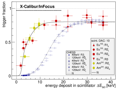
Figure 20: Fraction of CZT events with a scintillator coincidence trigger ($f_{\rm{sci}}=1$) as a function of energy deposition $\Delta E_{\rm{sci}}$. Data were taken with Am²⁴¹, Eu¹⁵², and at the CHESS beam (Sec. 8.1, however with a much higher scintillator threshold). The Compton-scattered continua (above background, see for example Fig. 19) were used to derive the trigger efficiency for different $\Delta E_{\rm{sci}}$. The distribution was fitted by a function shown in Eq. (14). The dashed horizontal line indicates the range of scintillator energy depositions for incoming X-rays in the $20-80\,\rm{keV}$ band.

The raw scintillator trigger rate (independent of CZT event triggers) of the optimized threshold setting of DAC=10 was measured to be only a few hundred Hz – a further reduction in trigger threshold by updating the signal amplifier seems possible and is work in progress.

A cleaner setup to measure the scintillator response is the well-collimated X-ray beam at CHESS (see Sec. 8.1). The results are also shown in Fig. 20 for a non-polarized beam at $40\,\rm{keV}$ and $120\,\rm{keV}$, respectively. However, the amplifier for the PMT reading the scintillator was not optimized at the time of the CHESS measurements, so that the $50\%$ trigger probability is only reached around $\Delta E_{\rm{sci}}\simeq 15\,\rm{keV}$. The corresponding fitted trigger efficiency (again with the $a=1$ assumption) was fed into the simulations that were done for the CHESS measurements discussed in Sec. 8.1.

7.3 Summary of the Instrument Characteristics

The rejection power of the active shield was studied in the laboratory. It reduces the background by more than one order of magnitude in the energy range relevant for X-Calibur.

When we require a scintillator trigger ($f_{\rm{sci}}=1$), the effective energy threshold of the polarimeter increases to $\simeq 25\,\rm{keV}$ (with the current scintillator threshold of $\sim$$5\,\rm{keV}$). We are working on a further reduction of the scintillator threshold Fabiani et al. [2013]. Above an energy of $30\,\rm{keV}$, we can detect a high fraction of events with a coincident scintillator signal. For ground-based background measurements, the scintillator coincidence reduces the background by another factor of $\sim$$30$. On upcoming balloon flights, we will use events with (for best high-energy signal to noise ratio) and without (for best low-energy response) scintillator coincidences.

8 X-Calibur: Polarization Measurements

This section discusses measurements performed with the fully assembled and calibrated X-Calibur polarimeter. Measurements of non-polarized and polarized X-ray beams at the CHESS facility at Cornell University are described in Sec. 8.1 and are compared to simulations. The results illustrate the functionality of X-Calibur as an X-ray polarimeter. Section 8.2 describes X-Calibur measurements that were taken with the fully integrated X-Calibur/InFOC$\mu$S X-ray telescope in Ft. Sumner during a test integration of a flight-ready balloon setup.

Systematic effects and asymmetries in the detector response can, under certain circumstances, cause measurements of aparent polatization fractions, even if the measured X-ray beam itself is non-polarized. It is therefore crucial to understand and control these kinds of systematic effects in order to correctly study the polarization properties of astrophysical sources. The systematic effects (and corrections thereof) caused by a X-ray beam hitting the polarimeter off-center are discussed in Sec. 8.3.

8.1 Polarized X-rays from the CHESS Beam

In order to measure the response to a polarized X-ray beam, the X-Calibur polarimeter was operated at the Cornell High Energy Synchrotron Source (CHESS) for one week in March 2013. CHESS provides a highly collimated and highly polarized beam of synchrotron X-rays. Using Bragg reflection from a 2-bounce silicon (220) monochromator, a $40\,\rm{keV}$ beam was generated with the 2^nd/3^rd harmonics at $80/120\,\rm{keV}$, respectively. The measurements were performed in hutch C1. The polarimeter was mounted on an adjustable X/Y/Z stage table with the scintillator being aligned with the X-ray beam (using X-ray fluorescence paper). The setup, referred to as $C_{\rm{ch}}$, is shown in Fig. 6. X-Calibur was mounted in a fixture that allowed us to rotate the polarimeter around the optical/beam axis, in order to test the response at different orientations between the polarization plane and the detector. The rotation angle is referred to as $\alpha$ with detector board Bd0 located at the top position at $\alpha=0^{\circ}$ (see $C^{3}$ in the top panel of Fig. 6). Looking into the beam, a positive angle $\alpha$ corresponds to a counter clock-wise rotation. The accuracy of setting the angle was estimated to be $\Delta\alpha\simeq 2^{\circ}$. It should be noted that we did not use a high precision rotation mechanism (as will be used during the balloon flight). Therefore, an $\alpha$ dependent mis-alignment/tilt of the scintillator during the measurements cannot be excluded.

The CHESS X-ray flux. A total of 30 synchrotron-emitting electron bunches cycle the CHESS accelerator ring. The relative intensity of the X-ray beam entering the C1 hutch is controlled by a system of slits, as well as the tunable orientation of the Bragg reflection crystals. The intensity, however, varies with (i) decaying electron population in the ring during a run (re-charged every $\sim$$2\,\rm{h}$), (ii) local heat built-up on the Bragg crystals, and (iii) the position stability of the electron beam in the ring. The intensity of the monochromatic beam entering the hutch was monitored using an argon ion chamber ($6\,\rm{cm}$ in length along the beam, set to a counter range of $10^{-8}\,\rm{A}/\rm{V}$). The absolute flux calibration of X-Calibur was not a major objective of the measurements; therefore, we did not setup a system to automatically stabilize the beam intensity entering the hutch – but rather kept it manually in the ballpark of $1-2\cdot 10^{8}\,\rm{cts}/\rm{s}$ (ion chamber) throughout the measurements and logged the average intensity for each data run. Absorber foils placed behind the ion chamber further reduced the beam intensity by several orders of magnitude. This brought the X-ray flux hitting the polarimeter down to the level of $1-2\,\rm{kHz}$, a regime that can be well handled by the readout electronics of the polarimeter.

Configurations. An aluminum collimator plate of thickness $0.5^{\prime\prime}$ was placed directly in front of the X-Calibur polarimeter with an entrance hole of $0.25^{\prime\prime}$ in diameter. The CZT detector configuration used for the CHESS measurements is listed in Tab. 1. CHESS data presented in this paper were taken with three configurations (variations of $C_{\rm{ch}}$ as depicted in Fig. 6).

$C_{\rm{ch1}}$: the absorber foils consist of platinum (Pt), a $125\,\mu\rm{m}$ layer placed directly after the ion chamber and a stack of four $90\,\mu\rm{m}$ layers placed between the ion chamber and X-Calibur. This setup is optimized for a band-pass at $40\,\rm{keV}$.

$C_{\rm{ch3}}$: One layer of $125\,\mu\rm{m}$ Pt absorber foil is placed directly behind (downstream) the ion chamber, and a $1.27\,\rm{mm}$ lead foil (Pb) is placed between the ion chamber and X-Calibur. This setup is optimized for a band-pass at $80\,\rm{keV}$.

$C_{\rm{ch4}}$: Same as $C_{\rm{ch3}}$, but the ion chamber was removed from the beam path (in order to extend the range of beam offsets without interfering with the housing of the ion chamber).

X-Calibur detects individual events, but only the ASIC that triggered the event (corresponding to $1/64$ of the polarimeter) is dead during the read-out which takes $\sim$$130\,\mu\rm{s}$. The dead-time during data runs is therefore usually not higher than $5\%$. In order to guarantee a homogeneous data set, some additional pixels (as compared to the calibration runs) were excluded from the analysis which had high thresholds or were too noisy – even though the azimuthal acceptance (see Sec. 4) is in general capable of correcting for most of these effects. Only events with multiplicity $m=1$ pixels were selected. X-Calibur was not operated in its active CsI shield, and the scintillator PMT discriminator was not yet optimized at the time of the CHESS measurements.

Data runs. A series of measurements was taken with configuration $C_{\rm{ch1}}$ (optimized for $40\,\rm{keV}$) and $C_{\rm{ch3,4}}$ (optimized for $80\,\rm{keV}$). Data were taken with different polarimeter orientations $\alpha$. The $C_{\rm{ch1}}$ data runs span a range of $\alpha\in[-90;+90]^{\circ}$ in steps of $10^{\circ}$ with $4\,\rm{Mio}$ events per orientation. A non-polarized beam was ‘generated’ by the superposition of data from two perpendicular orientations. A higher number of events were taken for these sets: $20\,\rm{Mio}$ events for the $\alpha=0/-90^{\circ}$ pair, and $10\,\rm{Mio}$ events for the $\alpha=\pm 45^{\circ}$ reference pair. The $C_{\rm{ch3,4}}$ series scanned a range of $\alpha\in[-90;+10]^{\circ}$ with a non-polarized beam composed from $10\,\rm{Mio}$ events derived from the $\alpha=0/-90^{\circ}$ orientations.

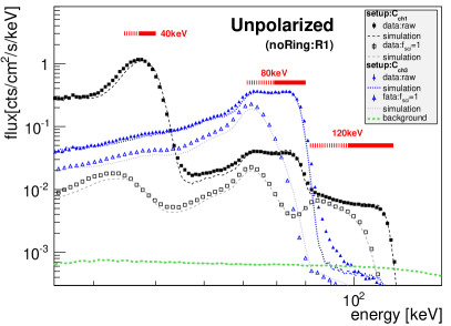
Figure 21: Energy spectra of the Compton-scattered non-polarized CHESS X-ray beam (superposition of perpendicular polarization planes). The measurements were performed with the two configurations $C_{\rm{ch1}}$ and $C_{\rm{ch3}}$ (see text and Fig. 6). Shown are the background subtracted integral spectra of all detectors – only ring R1 was excluded due to flux contamination (see text and Fig. 22, right, for the reason). The background level is shown for reference. The horizontal lines represent the nominal energies of the three harmonics for (left to right): $180-90^{\circ}$ Compton-scattering (dotted), and $90-0^{\circ}$ Compton-scattering (solid). Spectra are shown with and without the $f_{\rm{sci}}=1$ scintillator coincidence requirement. Simulated spectra are shown, as well.

Several background runs were taken without the X-ray beam entering the hutch. The over-all background spectrum is shown in the left panel of Fig. 17 (red data points). The C1 hutch is shielded by (partly) lead-enforced walls which likely contribute to the lower background level as compared to the laboratory at Washington University. In fact, a signature at the lead $\rm{KL}_{1-3}$ transition energies can be identified in the CHESS background spectrum. Although the background is negligible compared to the strong X-ray signal (see Figs. 22 and 23 for reference), it was subtracted from the spectra shown in this section. It should be noted that the beam in the hutch may introduce an additional implicit/diffuse background by scattering off several components (slits, absorber foils, etc.). This kind of background was not determined in a dedicated measurement, but can potentially be higher than the CR background.

Synchronization between simulations and data. The Bragg monochromator only allows the $40/80/120\,\rm{keV}$ harmonics of the CHESS white beam to enter the C1 hutch. The spectral intensities of the white beam, as well as the Bragg-reflected intensities of the monochromator, were calculated using the X-ray Oriented Programs (XOP) software package. The absorber foils further change the relative intensities. Given the density of platinum of $\rho_{\rm{Pt}}=21.45\,\rm{g}/\rm{cm}^{3}$, its mass attenuation coefficient at $40\,\rm{keV}$ of $(\mu/\rho)_{\rm{Pt}}=12.45\rm{cm}^{2}/\rm{g}$, and the thickness of the Pt foils $d$, one can calculate the beam intensity $I$ entering the polarimeter by $I/I_{0}=\exp(-\mu/\rho\cdot\rho\cdot d)$. The mass attenuation coefficients $\mu/\rho$ were taken from the NIST X-ray database. However, an accurate prediction of the relative flux intensities entering the polarimeter requires a detailed modeling of all energy-dependent X-ray absorption/transmissions on the beam path (including the entrance windows, the Bragg monochromator, and the absorber foils).

Therefore, we instead used the overall spectrum measured by the whole polarimeter to synchronize the relative $40/80/120\,\rm{keV}$ flux intensities with our Monte Carlo simulations. Figure 21 shows the overall X-Calibur responses (all detector rings except for R1, see below) to the non-polarized CHESS beam, measured with configurations $C_{\rm{ch1}}$ and $C_{\rm{ch3}}$. The corresponding relative intensities of the three mono-energetic energies in the simulations were matched accordingly and are in turn applied for all data versus simulation comparisons that follow. Note, however, that the CHESS white beam intensity varies. Therefore, the simulations were scaled according to the relative difference in the integral X-Calibur trigger rate with respect to the data run used to normalize the simulations. We estimate the systematic error on the absolute flux normalization of the simulations to be around $20\%$. Figure 21 also shows the energy spectra with a coincident scintillator trigger ($f_{\rm{sci}}=1$), although obtained with the non-optimal scintillator trigger threshold.

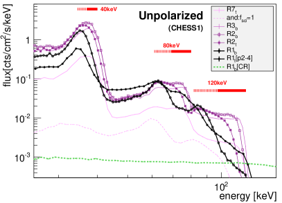
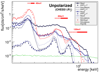
Figure 22: Energy spectra of the Compton scattered, non-polarized $40/80/120\,\rm{keV}$ CHESS X-ray beam (averaged over the complete azimuthal scattering range, $m=1$ events). The horizontal lines represent the nominal energies after Compton-scattering. For reference, the CR spectrum is shown for one of the $5\,\rm{mm}$ rings. Left: Spectra from selected sub rings. In the case of ring R1_t, the first pixel row was removed (see text and right panel). Right: Special case of ring R1_t which is located at the polarimeter entrance; individual pixel rows are shown. It can be seen that the first pixel row has significantly higher flux at $E>40\,\rm{keV}$ as compared to the other rows – likely due to external X-ray contamination. The same spectra are shown with the scintillator trigger condition ($f_{\rm{sci}}=1$). Simulated spectra are shown for the pixel rows 1 and 4. The spectrum obtained from the first pixel row in Ring R2_t is shown for reference.

Compton spectra of a non-polarized beam. The energy spectra of the non-polarized Compton scattered X-ray beam are shown for individual detector rings in Fig. 22 (left). The spectra are averaged over all azimuthal scattering angles $\Phi$ within each ring. Ring R1_t mostly detects back-scattered events (the scintillator geometrically covering rings R2-R8, see Fig. 3, left) which deposit the maximal amount of energy in the scintillator: $\Delta E_{\rm{sci}}$ up to $5.4\,\rm{keV}$ for the $40\,\rm{keV}$ beam, depositing $E_{\rm{czt}}=34.6\,\rm{keV}$ in the CZT detector. The rings further downstream detect a superposition of X-rays that underwent Compton-scattering under different angles. The rear-side rings (R7 and R8), to a larger extent, detect X-rays which Compton scattered nearly in the forward direction – depositing only a small amount of energy in the scintillator, with an energy deposition in the CZT ($E_{\rm{czt}}$) close to the energy of the primary X-ray ($E_{\rm{line}}$). This explains the shift of the peak positions in the spectra towards higher energies with increasing ring number. The theoretical range expectations of $E_{\rm{czt}}$ are indicated by the horizontal lines in Fig. 22 (assuming an idealized energy resolution).

The right panel of Fig. 22 shows the energy spectra of individual pixel rows of ring R1_t. It can be seen that the first pixel row shows a strong anomaly at energies $E_{\rm{czt}}>50\,\rm{keV}$ as compared to the pixel rows 2-4. The comparison with simulations further underlines the difference. A likely explanation of the additional continuum would be the following. The first row of pixels has a rather high effective area (pixel sides) in the plane perpendicular to the X-ray beam, as compared to other pixel rows. These ‘side’ pixels will detect X-rays that underwent diffuse scattering in the Pt/Pb absorber foils or the polarimeter entrance plate (see Fig. 6), and succeeded in entering the polarimeter along a path not along the optical axis. Since this involves X-ray transmission through some of the material of the polarimeter fixture, it is more likely to happen for higher energies, which is where the anomaly in the spectrum becomes more prominent. The first pixel row was therefore excluded from the analysis of the data presented in this section. It should be noted, that the contamination is also seen in the pixel rows further downstream – however, with strongly decreasing strength.

The right panel of Fig. 22 also shows the spectra obtained from the same data with the additional requirement of a scintillator trigger ($f_{\rm{sci}}=1$). This favors high-energy and/or back-scattered events which deposit a high amount of energy $\Delta E_{\rm{sci}}$ in the scintillator. With the $f_{\rm{sci}}=1$ cut, the first pixel rows no longer show the anomaly discussed above – underlining the hypothesis of an external contamination not interacting with the scintillator. A more detailed study of the trigger efficiency of the scintillator is presented in Sec. 7.2. Despite the contamination issue seen in the first front-side pixel rows, the Compton-spectra measured with X-Calibur are in good agreement with the simulations (although not explicitly shown for all rings in Fig. 22, right, for reasons of visibility.).

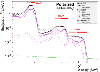
Figure 23: Compton spectra of the polarized $40/80/120\,\rm{keV}$ CHESS beam. Spectra are shown for two of the four detector sides (Bd0 and Bd1, see Fig. 6, top) in ring R2_b, with Bd0 aligned with the plane of polarization ($\alpha=0^{\circ}$). The Bd1 spectrum is also shown with the requirement of a scintillator trigger (the discriminator threshold not being optimized at this point). The horizontal lines represent the nominal energy ranges after Compton-scattering. The simulated spectra are shown, as well.

Compton spectra of a polarized beam. A polarized X-ray beam introduces an azimuthal modulation with a $180^{\circ}$ periodicity to the measured spectra. Figure 23 shows the Compton spectra measured on two of the four detector sides in ring R2_b (with the polarimeter being oriented at an angle of $\alpha=0^{\circ}$). As expected, and essential for the functionality of the polarimeter, the detector side located perpendicular to the polarization plane (Bd0) detects a higher number of Compton-scattered X-rays. The energy spectra obtained from simulations are shown in Fig. 23, as well, and are found to be in reasonable agreement with the data. For the data versus simulation comparison one has to keep in mind that the simulations were performed for a $100\%$ polarized beam, corresponding to the maximal modulation and therefore a maximal scattering concentration in Bd0. The polarization fraction of the CHESS beam, on the other hand, is $r<100\%$. Therefore, the azimuthal asymmetry (Bd0 versus Bd1) in the data is expected to be smaller compared to the simulations. Dividing the spectra into distinct bins in azimuth, and integrating counts in a given energy interval, will lead to the azimuthal scattering distributions that are discussed in the next paragraph.

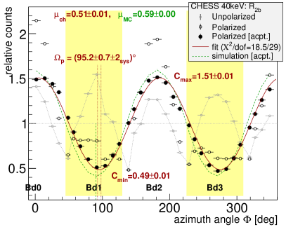
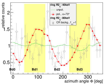
Figure 24: Left: Azimuthal scattering distribution (CHESS at $40\,\rm{keV}$, ring R2_b). The horizontal error bars reflect the azimuthal ranges $\Delta\Phi_{j}$ covered by the corresponding pixels $j$ (see Fig. 8, left). The raw non-polarized beam shows the 4-fold symmetry of the four detectors boards Bd0-Bd3 (see Fig. 6). The polarized beam has the additional $180^{\circ}$ amplification imprinted which is clearly extracted once corrected for the azimuthal coverage $\Delta\Phi_{j}$ and the pixel acceptance $a_{j}$. A sine function is fitted to extract $C_{\rm{min}}$, $C_{\rm{max}}$, the modulation factor $\mu$, and the angle of the polarization plane $\Omega_{\rm{p}}$ (dotted vertical lines, indicating the error range). The dashed vertical line indicates the nominal polarization plane. For reference, the distribution of a simulated $40\,\rm{keV}$ beam is shown ($100\%$ polarized, reconstructed in the same way). Right: Normalized azimuthal scattering distributions derived from different data sets: a non-polarized beam, a polarized beam measured at $\alpha=70^{\circ}$, as well as the response to a cosmic-ray background run.

Azimuthal scattering distribution. The azimuthal scattering distributions were generated as outlined in Sec. 4.4 by integrating the energy range of Compton-scattered photons for the three harmonics of the X-ray beam ($34.6-40\,\rm{keV}$, $60.9-80\,\rm{keV}$, and $81.7-120\,\rm{keV}$, respectively). The energy intervals include an additional $2\,\rm{keV}$ cushion to account for the energy resolution of the CZT detector pixels. All measured event rates were in turn normalized on a pixel-by-pixel basis using the azimuthal coverage $\Delta\Phi_{j}$ and acceptances $a_{j}$. Following Eq. (5) described in Sec. 4.4, the pixel acceptances $a_{j}$ were determined from the non-polarized beam for each of the above energy intervals.

An example of an azimuthal scattering distribution measured in the $34.6-40\,\rm{keV}$ band is shown in Fig. 24 (left). The normalized distribution is used to derive the plane of polarization $\Omega_{\rm{p}}$ (nominal value of $\Omega_{\rm{nom}}=90^{\circ}$), as well as the relative scattering amplitude $\mu_{\rm{ch}}$. The distribution is compared to the one obtained from the simulation of a $100\%$ polarized beam at $40\,\rm{keV}$. Both are found to be in good agreement – except for the slightly lower amplitude of the data which is a result of the $r<100\%$ polarization fraction of the CHESS beam (see below).

Figure 25 illustrates the reconstruction of the azimuthal scattering distributions for the complete polarimeter (subrings R1_t-R8_b), based on simulations (top panel) and based on measured CHESS data (bottom panel). The response to a non-polarized $40\,\rm{keV}$ beam is shown on the left side of the figure. The second panel shows the polarimeter response to a polarized beam at $40\,\rm{keV}$, not yet corrected for pixel acceptance $a_{j}$ and azimuthal coverage $\Delta\Phi_{j}$. Applying the corrections leads to the smooth distribution shown in the third panel, which is in good agreement if comparing the simulations to the data. The pixel acceptances $a_{j}$ depend on (i) the energy threshold, (ii) the energy resolution, and (iii) the trigger efficiency of the pixel $j$. The simulations take into account (i) and (ii), derived from the calibration measurements presented in Sec. 6.1, but not (iii). The projected count distributions lead to the azimuthal scattering distributions shown in the right panel of Fig. 25. In contrast to the 2D distributions shown in planar pixel coordinates, the $\Phi$ positions and error bars now represent the proper angular coverage of each pixel (compare with Fig. 8, left). The expected $180^{\circ}$ modulation is clearly revealed, and the reconstructed orientation of the polarization plane agrees with the direction of the CHESS beam setup – confirming the functionality of the X-Calibur polarimeter.

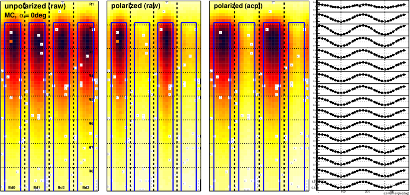
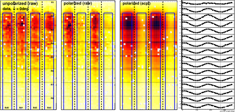
Figure 25: X-Calibur 2D scattering distributions of the $40\,\rm{keV}$ beam at CHESS ($C_{\rm{ch}}^{3}$, see Fig. 6, the beam enters from the top). Events are shown for reconstructed energies of $36-40\,\rm{keV}$. The top row shows the results of simulations of a $100\%$ polarized beam. The bottom row shows the results of the CHESS measurement. The (blue) boxes in the 2D maps indicate the projected outline of the scintillator (Compton-scatterer). Left: Raw count map (pixel-by-pixel) of a non-polarized beam (neither corrected for $\Delta\Phi_{j}$ nor for pixel acceptance $a_{j}$). All four detector sides, Bd0-Bd3, are unfolded into a plane. The detector rings R1 to R8 are indicated. Second: Count map of a raw measurement of a polarized beam. Third: Count map of the polarized beam, corrected for $\Delta\Phi_{j}$ and $a_{j}$. Right: Normalized azimuthal scattering distribution (corrected for $\Delta\Phi_{j}$ and $a_{j}$) for different detector rings. The vertical lines indicate the nominal plane $\Omega_{\rm{n}}$ of the electric field vector of the polarized beam.

Simulated modulation factors. Each detector ring (see Fig. 25), or a sub ring thereof, can be seen as an independent detector that allows to reconstruct energy-dependent polarization properties of the incoming X-ray beam. Figure 26 shows the simulated modulation factors $\mu_{\rm{sim}}$ for the different energies and X-Calibur configurations as a function of detector ring/depth, measured along the optical axis. The values for $\mu_{\rm{sim}}$ were obtained using the Stokes analysis, and are in agreement with the corresponding results obtained from the analysis of the azimuthal scattering distribution (not shown). The simulations shown reflect the detector status of the CHESS measurements (dead pixels, energy resolutions, etc.), not an idealized detector. Ring R1 detects only back-scattered X-rays with a correspondingly lower $\mu_{\rm{sim}}$ – but with a better energy resolution since the scattering kinematics are better defined. The step-like structure in $\mu_{\rm{sim}}^{120\,\rm{keV}}$ between rings R5 and R6 can be explained by the strong degradation in energy resolution at high energies in the $2\,\rm{mm}$ detectors located at rings R6-R8. The highest modulation is achieved in ring R2.

The simulations of the modulation factor were also done involving the scintillator flag $f_{\rm{sci}}$, based on the two scintillator trigger efficiencies as measured in Fig. 20. This reflects the efficiency during the CHESS measurements (not optimized), as well as the efficiency of the optimized scintillator trigger. The scintillator improves the modulation factor for most rings – by requiring a minimum energy deposition $\Delta E_{\rm{sci}}$ which effectively limits the allowed range of polar scattering angles. This, however, also reduces the event statistics (not imprinted in $\mu_{\rm{sim}}$). A scintillator trigger efficiency of $100\%$ would again lead to the same distribution of modulation factors as no cut on $f_{\rm{sci}}$ does. The main benefit of the scintillator trigger lies in its ability to suppress background during a measurement (see for example Fig. 17, left). The modulation factor $\mu$, together with the detection rate after background subtraction, are the crucial characteristics that determine the MDP detection sensitivity of the polarimeter following Eq. (4).

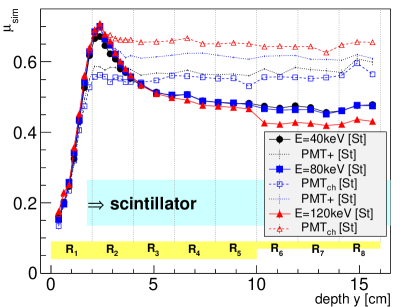
Figure 26: Simulated modulation factors $\mu_{\rm{sim}}$ as a function of detector ring R, shown for different energies. The geometrical positions (along the optical axis $y$) are indicated for the scintillator and the CZT ring assembly. The simulated data were analyzed with the Stokes method. Results are also shown for the scintillator trigger requirement $f_{\rm{sci}}=1$, assuming the PMT trigger efficiency during the CHESS measurements (PMT_ch) and the efficiency of the optimized PMT threshold (PMT+), see Fig. 20.

Polarization fraction of the CHESS beam. The azimuthal scattering distributions for each sub ring and each data set were fitted to determine $\mu_{\rm{ch}}$. The simulated modulation factors $\mu_{\rm{sim}}$ (Fig. 26) were in turn used to determine the polarization fraction $r$ of the CHESS beam using Eq. (6). This is shown in Fig. 27 for the $40\,\rm{keV}$ beam for different orientations $\alpha$ of the polarimeter relative to the polarization plane. Also shown are the residuals between the reconstructed polarization plane and the nominal polarization plane. Note, that for large values of $\alpha$ the azimuthal scattering distribution shows an additional global slope, possibly caused by an $\alpha$-dependent tilt of the rotation fixture (see Fig. 24, right, for an example orientation of $\alpha=70^{\circ}$). This will affect the reconstructed polarization properties and is further discussed in Sec. 8.3. To reduce this systematic effect, the CHESS azimuthal distributions were folded back into the $[0;180]^{\circ}$ interval before the sinusoidal function was fitted to the data points.

Setup	$\Delta\Omega\,[\rm{deg}]$	$r_{\rm{rec}}\,[\%]$
beam energy: $40\,\rm{keV}$
$C_{\rm{ch1}}$	$-4.7\pm 1.9$	$91.0\pm 0.6$
	$-4.6\pm 1.7$	$88.6\pm 0.4$
beam energy: $80\,\rm{keV}$
$C_{\rm{ch1}}$	$-2.6\pm 1.7$	$83.5\pm 0.8$
	$-2.0\pm 2.1$	$78.3\pm 0.8$
$C_{\rm{ch1}}$, $f_{\rm{sci}}=1$	$-2.1\pm 2.5$	$86.5\pm 1.1$
	$-2.1\pm 2.7$	$82.8\pm 1.0$
$C_{\rm{ch4}}$	$-2.5\pm 1.8$	$90.4\pm 0.5$
	$-2.0\pm 2.2$	$85.5\pm 0.6$
beam energy: $120\,\rm{keV}$
$C_{\rm{ch1}}$	$-0.5\pm 2.9$	$89.2\pm 1.5$
	$-0.2\pm 3.3$	$71.5\pm 1.3$
$C_{\rm{ch1}}$, $f_{\rm{sci}}=1$	$-0.7\pm 4.6$	$86.3\pm 1.2$
	$-0.8\pm 3.7$	$80.5\pm 1.5$

Table 3: Residuals between the reconstructed polarization plane $\Omega_{\rm{p}}$ and the nominal plane at $\Omega_{\rm{n}}=90^{\circ}$: $\Delta\Omega=(\Omega_{\rm{n}}-\alpha)-\Omega_{\rm{p}}$. The second column shows the reconstructed polarization fractions $r_{\rm{rec}}$ of the CHESS beam at different energies and different configurations/setups (partly with the $f_{\rm{sci}}=1$ requirement). See Figs. 27 and 28 for an illustration. The first row per data set shows the results obtained from the analysis of the azimuthal $\Phi$-scattering distribution following Eq. (6). The second row represents the results obtained from the Stokes analysis following Eq. (11). The results are averaged over all orientations $\alpha$, each.

Figure 28 shows the corresponding polarization fractions reconstructed from the $80\,\rm{keV}$ harmonic. The reconstructed polarization fractions obtained from all measurements are summarized in Tab. 3 – in all cases averaged over all measured orientations $\alpha$. Table 3 also shows the results derived from the Stokes analysis following Eq. (11). Both methods are in reasonable agreement, whereas the Stokes analysis seems to slightly underestimate $r$ compared to the results obtained with the azimuthal scattering distribution. The systematic error on the reconstructed polarization fraction was estimated as described in Sec. 8.3. The polarization of the CHESS beam as reconstructed using the $\Phi$-distribution method is measured to be $r_{\rm{ch}}^{\Phi}=(87.8\pm 0.4_{\rm{stat}}\pm 4.6_{\rm{sys}})\,\%$ with no indication of an energy dependence in the $40-120\,\rm{keV}$ range. The corresponding value reconstructed from the Stokes analysis is $r_{\rm{ch}}^{\rm{st}}=(81.2\pm 0.4_{\rm{stat}}\pm 10_{\rm{sys}})\,\%$. The difference in the systematic error is explained by the fact that the Stokes analysis is more sensitive to the detector configuration (which was not perfectly constrained during the CHESS measurements). A better defined geometry and the rotation of the polarimeter will reduce the systematic error for measurements performed during the balloon flight.

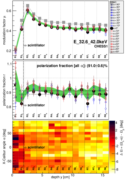
Figure 27: Reconstructed polarization properties of the CHESS beam at $40\,\rm{keV}$ (configuration $C_{\rm{ch1}}$). Top: Modulation factor $\mu$ versus polarimeter sub rings Ri_t,b. The results were derived from simulations (MC), as well as from data taken under different X-Calibur orientations $\alpha$. For each $\alpha$ and each ring, $\mu_{\rm{ch}}$ is derived from fits to acceptance corrected $\Phi$-distributions (see Fig. 24, left). The scintillator starts covering detector rings at $y\geq 1.8\,\rm{cm}$. The green error band reflects the $1\,\rm{std.dev}$ range of measured points in the particular $y$ slice. Middle: Reconstructed polarization fraction following Eq. (6). The green band reflects the $1\,\rm{std.dev}$ range of all reconstructed fractions in the corresponding $y$ slice. Bottom: Residual between reconstructed polarization plane $\Omega_{\rm{p}}$ and true polarization plane $\Omega_{\rm{n}}=90^{\circ}$, corrected for the X-Calibur orientation $\alpha$: $\Delta\Omega=(\Omega_{\rm{n}}-\alpha)-\Omega_{\rm{p}}$.

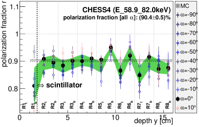
Figure 28: Reconstructed polarization fractions of the CHESS beam (compare with Fig. 27) derived from the $80\,\rm{keV}$ harmonic (configuration $C_{\rm{ch3}}$).

Polarization plane of the CHESS beam. Table 3 also summarizes the average reconstructed polarization planes $\Omega_{\rm{p}}$ (corrected for the X-Calibur orientation $\alpha$). Note, that the uncertainty in setting the X-Calibur orientation was estimated to be $\Delta\alpha=\pm 2^{\circ}$. Within this systematic error, as well as the statistical errors, the average of reconstructed polarization planes (all rings and all X-Calibur orientations $\alpha$) is compatible with the nominal plane $\Omega_{\rm{n}}$ of the CHESS beam. However, the measurements consistently reconstruct $\Delta\Omega<0^{\circ}$, which may indicate a slight offset in the way the rotation mechanism was installed/calibrated. The reconstructed polarization planes shown in Fig. 27 indicate a slight dependence on $\alpha$ and $y$. The left panel in Fig. 24 shows a corresponding azimuthal distribution measured with the X-Calibur orientation of $\alpha=70^{\circ}$, revealing a slight asymmetry. This result can be seen as another indication of a slight mis-alignment (offset and/or tilt) between the rotation axis of the scintillator and the optical axis of the X-ray beam. A more detailed discussion of this kind of systematic effect can be found in Sec. 8.3.

8.2 Measurements with the X-Calibur/InFOC$\mu$S Assembly

The full X-Calibur/InFOC$\mu$S experiment was assembled and tested during a flight preparation campaign at the NASA Columbia Scientific Balloon Facility (CSBF) site in Ft. Sumner, NM, in the fall of 2014. The polarimeter was installed in the rotating CsI shield assembly, which in turn was installed in the pressure vessel as part of the InFOC$\mu$S X-ray telescope (see Fig. 5). This setup, $C_{\rm{ft}}$, is illustrated in Fig. 6. The CZT detector configuration of these measurements is listed in Tab. 1 and differs slightly from the one used in the CHESS measurements (described in Sec. 8.1). The X-ray mirror was installed on the optical bench located at the front part of the InFOC$\mu$S telescope. The pressure vessel is located at a focal distance of $8\,\rm{m}$.

Before the balloon flight, a beryllium (Be) window is installed in the top dome of the pressure vessel, to assure a pressure-sealed entrance to the polarimeter with high transmissivity to hard X-rays. For the ground-based measurements, presented in this section, the Be window was not installed to allow to visually align the polarimeter with the optical axis of the X-ray mirror. Throughout the measurements presented in this section, the polarimeter was rotated at $4\,\rm{rpm}$. Due to the rotation, the application of the pixel acceptances $a_{j}$, defined in Eq. (5), is no longer required, since each pixel tests the complete, time-averaged azimuthal scattering range with respect to the polarization plane. As another consequence, the azimuthal binning can be chosen finer than in the non-rotating system in which it was limited to the number of $32$ CZT pixels per row. For each event, the hit pixel is de-rotated into the laboratory/horizon coordinate frame (see Fig. 8, left) to determine the azimuthal scattering angle $\Phi$.

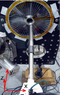
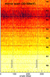
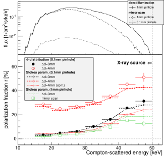
Figure 29: InFOC$\mu$S/X-Calibur X-ray mirror scan, configuration $C_{\rm{ft}}$ in Fig. 6. Left: The collimated X-ray source is aligned with the optical axis of the mirror and the polarimeter which is situated in the focal plane at a distance of $8\,\rm{m}$ (not visible in this photograph). The X-ray source can be automatically moved in the $X$/$Z$ plane to scan the mirror with the X-rays traveling along $Y$. Middle: The Compton-scattered event distribution measured with X-Calibur (horizon system, de-rotated) during the scan in the energy range of $30-50\,\rm{keV}$. Right: Background subtracted measurements of the collimated X-ray beam. Three data runs where taken with (i) the beam hitting the center of the scintillator ($\Delta d=0\,\rm{mm}$), (ii) the beam hitting at an offset of $\Delta d=-4\,\rm{mm}$, and (iii) the beam scanning the X-ray mirror. The top panel shows the Compton-scattered energy spectra (all-detector average, each). The bottom panel shows the energy-dependent polarization fraction reconstructed from the azimuthal $\Phi$-scattering distribution, as well as using the Stokes parameters. The given errors are statistical only.

X-ray mirror/X-Calibur alignment. The alignment of the polarimeter and the mirror are crucial in order to gain the maximal sensitivity for polarization measurements and to reduce systematic effects. The optical axis and the on-axis image location of the X-ray mirror were measured by a CCD camera with an optical parallel beam. The X-ray mirror was placed in the optical beam, and its tip and tilt were adjusted such that the optical axis is parallel to the optical beam. Then, the CCD camera was placed at the center of the mirror, looking along the optical axis facing the polarimeter, and taking a picture of the on-axis image plane. The image location was recorded in pixel coordinates, which determines the optical axis as well as the on-axis image position. After the X-ray mirror was installed onto the optical bench (see Fig. 29, left), a picture of the front surface of the polarimeter’s scintillator was taken by the camera. The mirror tip and tilt were adjusted by shimming at the interface to the optical bench, such that the center of the scintillator is at the recorded location of the on-axis image of the X-ray mirror. An alignment between the scintillator and mirror of better than $1\,\rm{mm}$ was achieved which guarantees a systematic error on the reconstructed polarization fraction of less than $2\%$ (see Sec. 8.3).

Mirror scan. The proper alignment of the telescope is tested/confirmed in a mirror scan. A movable X-ray source scans the surface of the mirror while the polarimeter response is measured. The X-ray scanning system consists of an X-ray source with a $60\,\rm{cm}$ long collimator, tip and tilt stages, and $X$/$Z$ travel stages to which the X-ray source is mounted. The X-ray source was positioned in front of the X-ray mirror and could be used to either directly illuminate the polarimeter (through the central hole in the X-ray mirror), or to scan the whole mirror aperture. The setup is shown in Fig. 29, left. An Oxford 5011 electron impact X-ray tube is used to generate the X-rays, with an active source spot size of $0.05\,\rm{mm}$ in diameter (molybdenum target, Mo). The produced X-ray spectrum is made of emission line (Mo-K) as well as bremsstrahlung. The X-ray source provides a continuum spectrum up to $50\,\rm{keV}$. The current was adjusted to give a reasonable event rate at the polarimeter located at $8\,\rm{m}$ distance (see Tab. 2 for reference). The collimator can be equipped with two interchangeable pin holes with diameters of $0.1\,\rm{mm}$ and $1\,\rm{mm}$, respectively. The beam size at $8\,\rm{m}$ distance is around $2\,\rm{mm}$ in diameter for the $0.1\,\rm{mm}$ pin hole. The $1\,\rm{mm}$ pin hole produces count rates in the polarimeter above one kHz at $8\,\rm{m}$ distance ($20-50\,\rm{keV}$, after air absorption). The tip and tilt stages change the direction of the collimated X-ray beam. The $X$/$Z$ translation stages allow the X-ray beam to scan over the entire aperture of the mirror (with the central hole in the mirror blocked by a lead absorber). The X-ray beam was aligned with the optical axis of the mirror. The $1\,\rm{mm}$ pin hole was used to scan the mirror within $51$ horizontal rows along $X$. The response measured with X-Calibur is shown in Fig. 29 (middle) in the de-rotated coordinate system (the horizon intersects at $90^{\circ}$ and $270^{\circ}$ in this representation). The corresponding energy spectrum is shown in Fig. 29, right. The results illustrate that the mirror was successfully aligned with the polarimeter.

Direct beam illumination. As a reference measurement to the mirror scan, data were taken with the polarimeter being directly illuminated by the collimated X-ray source ($0.1\,\rm{mm}$ pin hole). The X-rays enter the scintillator along its optical axis, but do not pass the X-ray mirror in this measurement. The spectrum of the mirror scan shown in Fig. 29 (right, top) drops off faster compared to the spectrum measured from the direct beam illumination. This is a result of the energy-dependent effective area of the mirror. An additional run was taken with the X-ray beam hitting the scintillator off center by $\Delta d=-4\,\rm{mm}$, which is discussed in Sec. 8.3.

The polarization parameters were reconstructed in the same way as described in Sec. 8.1 (except for the acceptance correction $a_{j}$). The depth-dependent modulation factors (see Fig. 26) obtained from the $40\,\rm{keV}$ CHESS simulation were used to reconstruct the polarization fraction of the X-ray beam in different energy bands (assuming $\mu_{\rm{sim}}$ being independent of energy in the $20-50\,\rm{keV}$ band). The reconstruction was done with both methods described in Sec. 4.4, namely using the analysis of the azimuthal scattering distribution following Eq. (6), as well as using the Stokes parameters following Eq. (11). Both methods yield comparable results which are shown in Fig. 29 (right, bottom). An energy dependent polarization fraction is found in the data. However, in contrast to the mono-energetic CHESS beam (Sec. 8.1), the energy distribution of the incoming X-rays (before Compton-scattering in the scintillator) follows a continuum. To properly reconstruct the polarization fraction as a function of incoming X-ray energy, one would have to utilize reconstruction methods of forward folding or unfolding Kislat et al. [2015a], which is beyond the scope of this paper. However, a significant increase in polarization fraction can be observed with increasing energy. The data of the mirror scan was also used to reconstruct the energy-dependent polarization fraction, and is found to be in reasonable agreement with the direct beam measurement. This confirms the predictions by Katsuta et al. [2009] that an X-ray mirror does not substantially affect the polarization properties.

8.3 Systematic Effects in Polarization Measurements

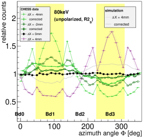
Figure 30: Left: Azimuthal scattering distributions of a non-polarized X-ray beam (CHESS data and simulations, both in a non-rotating system) hitting the scintillator at different offsets $d$ relative to the optical axis. X-Calibur was oriented at $\alpha=0^{\circ}$, with the beam ‘walking’ from Bd1 to Bd3 with increasing $\Delta X$ (see Fig. 8, left, for a coordinate system). Scattering distributions are shown with and without the offset correction (see Sec. 4.4). Right: Apparent polarization fraction $r$ of the non-polarized beam. The light blue region indicates the diameter of the scintillator rod. The data were analyzed using the Stokes parameters as described by Eq. (12). Results are shown without and with the corrected beam offset.

The understanding and control of systematic effects of different nature is crucial for the correct reconstruction of the polarization properties from measured data. A series of measurements was performed at CHESS (see Sec. 8.1) to study the effects of a mis-alignment (offset) between the X-ray beam and the optical axis of the polarimeter. The $X$/$Z$ stage of the table in hutch C1 was used to systematically scan the polarimeter response for offsets ranging from $-5\,\rm{mm}$ to $+5\,\rm{mm}$ in steps of $1\,\rm{mm}$ (the beam comes in along $Y$, see Figs. 6 and 8 (left) for the definition of the coordinate system). The scan along $X$ was performed with a polarimeter orientation of $\alpha=0^{\circ}$, whereas the scan along $Z$ was performed with $\alpha=-90^{\circ}$. This allowed us to pairwise superimpose the data runs of perpendicular polarization planes that hit the scintillator at the same position – being equivalent to a non-polarized beam hitting at that particular offset position. The data runs were taken with configuration $C_{\rm{ch4}}$, testing the response of the $80\,\rm{keV}$ harmonic of the CHESS X-ray beam. A set of simulations with an $80\,\rm{keV}$ beam (polarized and non-polarized) were performed resembling the same offsets as measured at CHESS, as well as offset simulations at $40\,\rm{keV}$.

Non-polarized beam. The left panel of Figure 30 shows examples of azimuthal scattering distributions measured with different beam offsets for a non-polarized beam. The distributions were corrected for $\Delta\Phi_{j}$ (assuming a central beam) and $a_{j}$, as before. It can be seen that beam offsets of $\simeq 2\,\rm{mm}$ already introduce systematic asymmetries. Although the offset distributions are not flat, as expected for a non-polarized beam, they also do not resemble the shape expected from a polarized beam. Given the high event statistics of the data used in the study, the sinusoidal fits used to determine the polarization properties will therefore certainly fail – allowing one to detect/filter the systematic effect. However, in the case of data with higher statistical uncertainty, the observed asymmetries could potentially lead to the reconstruction of an artificial polarization fraction of $r_{\rm{rec}}>0$. Note, that folding the distributions into the $[0;180]^{\circ}$ interval (not shown), will substantially reduce the asymmetry. The Stokes analysis is per definition only considering the $[0;180]^{\circ}$ interval. However, it is not sensitive to deviations from the sinusoidal scattering distribution, and therefore does not provide a goodness-of-fit measure that can be used to detect imprints of a beam offset. Figure 30 also shows examples of distributions that were offset corrected following the description in Sec. 4.4. This, however, assumes that the beam offset is known.

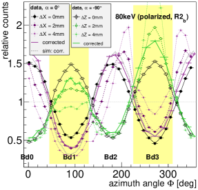
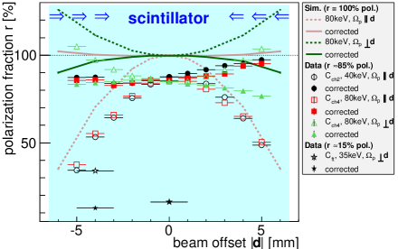
Figure 31: Left: Azimuthal scattering distributions of polarized X-ray beams hitting the scintillator at different offsets $d$. Results are shown for the CHESS data ($r_{\rm{ch}}\simeq 85\%$ polarized) and simulations ($r=100\%$ polarized), both in a non-rotating system. Distributions corrected for the beam offset (see Sec. 4.4) are shown, as well. Results are shown for offsets along $X$ ($\alpha=0^{\circ}$) and $Z$ ($\alpha=-90^{\circ}$, corresponding to a scan along $X$ with perpendicular polarization). Right: Reconstructed polarization fraction $r$ for the off-center beams, analyzed using the Stokes parameters as in Eq. (12). The outline of the scintillator is indicated. Also shown are data derived from the Ft. Sumner measurement shown in Fig. 29, right. Results are shown without and with the offset correction.

To quantify the artificial polarization $r_{\rm rec}$ inferred when neglecting the beam offset, the data were analyzed using the Stokes parameters following Eq. (12). Figure 30 (right) shows $r_{\rm{rec}}$ as a function of beam offset. The results are shown for the simulations as well as for the CHESS data – both being in reasonable agreement. Also shown is an analytic model that simply integrates the events per azimuth angle interval in a plane perpendicular to the optical axis. The right panel of Fig. 30 shows the same distribution after the beam offset correction described in Sec. 4.4 was applied. The discrepancy between the data and simulations after correction can be explained by an uncertainty in the absolute beam alignment in the data and the fact that, in contrast to the simulations, two separate measurements had to be superimposed to generate the non-polarized beam, amplifying the effect of unaccounted offsets or mis-alignments (any uncertainty in the offset not only moves the data points along the beam offset axis, but also along the $r$ axis).

In general, however, the first-order correction procedure greatly reduces the systematic effect to less than a few percent for offsets $d\leq 3\,\rm{mm}$. The simulated data shown in the right panel of Fig. 30 suggest that the correction works better for beam energies of $80\,\rm{keV}$ as compared to $40\,\rm{keV}$. This can be explained by the fact that only geometrical offsets are corrected for. Differences in absorption lengths in the scintillator material, originating from positions other than $P_{0}$ (see left panel in Fig. 8), will cause second-order effects that depend on the energy of the scattered X-ray. However, addressing these additional correction terms is beyond the scope of this paper.

Polarized beam. For a polarized beam (left panel in Fig. 31), the offsets lead to either a reduction or amplification of the reconstructed polarization fraction, depending on the angle between the offset vector $\bf{d}$ and the plane of polarization $\Omega_{\rm{p}}$. The contribution of the beam offset to the reconstructed polarization is illustrated in the right panel of Fig. 31 for different energies, including the results for the offset corrected analysis. The correction substantially reduces the systematic effect on $r$. A diverging trend can be identified in the corrected CHESS data for $d>0\,\rm{mm}$ (which is also visible in the case of the ‘non-polarized’ beam shown in the right panel of Fig. 30). This indicates an inaccuracy in the experimental setup, e.g. the asymmetric/fractional scattering off a fixture along the beam path before entering the polarimeter.

An additional offset measurement was performed during the flight preparation in Ft. Sumner (see Sec. 8.2) using the partly polarized beam of the collimated X-ray source, hitting the scintillator at an offset of $d=-4\,\rm{mm}$ (horizon system). The polarimeter/shield assembly was continuously rotating during the measurements. The corresponding fraction of apparent polarization $r$ is indicated in Fig. 31 (right). Due to the rotation of the polarimeter, the offset correction (see Sec. 4.4) was calculated on an event-by-event basis. The results illustrate that the correction also works in a rotated system, canceling the artificial fraction of polarization introduced by the offset. The offset-corrected polarization spectrum is shown in Fig. 29 (right), reproducing the measured results obtained with no beam offset.

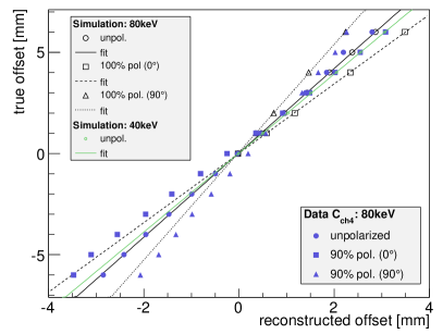
Figure 32: Correlation between true beam offset and beam offset measured following Eq. (15) for data and simulations.

Determination of the beam offset. The geometrical offset correction described above assumes that the offset vector $\bf{d}$ is known. For sufficient event statistics and the assumption of a time-independent beam offset, the offset can be estimated from the data itself using first moments, essentially substituting $2\Phi_{k}\rightarrow\Phi_{k}$ in Eq. (7):

$$\begin{split}\left<x\right>&=-\frac{c}{W}\sum_{k=1}^{N}w_{j(k)}\sin(\Phi_{k}),\\ \left<z\right>&=\frac{c}{W}\sum_{k=1}^{N}w_{j(k)}\cos(\Phi_{k}),\\ W&=\sum_{k=1}^{N}w_{j(k)}.\end{split}$$ (15)

Here, the constant $c=11\,\rm{mm}$ reflects the distance between the scintillator center and the detector plane (see Fig. 6, top). The weights $w_{j(k)}$ are the same as in Eq. (8). As shown in Fig. 32, the measured offsets are linearly correlated with the true beam offsets. However, the slope of the correlation depends to some extent on the true polarization fraction $r$ of the beam and the angle between $\Omega_{\rm{p}}$ and d. Since the offset of a non-polarized beam itself mimics a polarization fraction, there will be a residual ambiguity that prevents to completely disentangle $\bf{d}$ and $r$ from the data alone. Therefore, a time-resolved external monitoring of the beam position during the balloon flight is preferable.

Figure 32 reveals a slight shift/translation between the slope of the reconstructed offset measured in the CHESS data versus the slope obtained from the simulations. This can be used to estimate an accuracy of the alignment achieved during the CHESS measurements to be $\Delta X_{\rm{sys}}\simeq 0.3\,\rm{mm}$ for the X-Calibur orientation of $\alpha=0^{\circ}$. Note, with a rotation axis possibly not exactly aligned with the axis of the scintillator, this may translate into larger offsets $\Delta X$ for different X-Calibur orientations $\alpha$.

Systematic error on the polarization fraction. The systematic error on the reconstructed polarization fraction $\Delta r_{\rm{sys}}$ can be estimated as follows. For the polarization measurements presented in this paper (Sec. 8.1 and 8.2), we assume an unaccounted beam/scintillator mis-alignment of $\Delta d=1\,\rm{mm}$. For a highly-polarized beam of $r=O(100\%)$ this leads to an error of $\Delta r_{\rm{sys,\Delta d}}\simeq 2\%$ relative to the reconstructed on-axis beam (see simulated curve in Fig. 31). For a non-polarized beam (simulations in Fig. 30) the offset leads to an overestimation of $\simeq 2\%$. For simplicity, we describe the systematic error introduced by the beam offset as independent of the true polarization fraction: $\Delta r_{\rm{sys,\Delta d}}=2\%$.

The X-Calibur version used during the CHESS and Ft. Sumner measurements (see Secs. 8.1 and 8.2) allowed for some flexibility in adjusting the distance between the plane of the CZT detectors and the optical axis when assembling the polarimeter (see Fig. 6, top: $c=11\,\rm{mm}$). We measured $c_{\rm{ch}}=(11.3\pm 0.5)\,\rm{mm}$ for the CHESS setup and $c_{\rm{ft}}=(10.5\pm 0.5)\,\rm{mm}$ for the Ft. Sumner setup. Conservatively, we assume $c=(11\pm 1)\,\rm{mm}$. To study how an increased/decreased value of $c$ affects $r_{\rm{rec}}$, we correspondingly shifted pixel coordinates when analyzing a data set, but determined $r_{\rm{rec}}$ with the modulation factor $\mu_{\rm{sim}}$ obtained from simulations with the nominal value of $c=11\,\rm{mm}$. For $\Delta c=\pm 1\,\rm{mm}$, a $100\%$ polarized beam is reconstructed to be $r_{\rm{rec}}=r_{-0.5\%}^{+1\%}$ (overestimation for a reduced distance $c$). For a non-polarized beam the effect is estimated to be $<0.1\%$. We therefore assume that the distance related systematic error is proportional to $r$ with $\Delta r_{\rm{sys,c}}=0.01\,r_{\rm{rec}}$. In the case of the Stokes analysis, the uncertainty in $c$ will introduce another systematic error: the angular coverage of the detector gaps, corrected for by Eq. (10), will be over/underestimated. For a $100\%$ polarized beam and $\Delta c=-1\,\rm{mm}$, we find maximal deviation of $\Delta r_{\rm{sys,c}}^{\rm{Stk}}=\pm 6\%$, and for $\Delta c=+1\,\rm{mm}$ we find $\Delta r_{\rm{sys,c}}^{\rm{Stk}}=\pm 4.5\%$, with the sign and strength depending on the orientation of the detector planes relative to the polarization vector (see Sec. 4.4).

An error introduced by the analysis procedure can be estimated by comparing the results obtained with the two analysis methods presented in Sec. 4.4. No significant differences were found when analyzing simulated data of a non-polarized beam. Based on the modulation factors of a $100\%$ polarized beam, see Eq. (3), we estimate the systematic error to be on the order of $2\%$. Therefore, a relative error of $\Delta r_{\rm{sys,a}}=0.02\,r_{\rm{rec}}$ is assumed. Reasons for the difference can be the different treatment of dead pixels, detector gaps, etc. (see Sec. 4.4). The total systematic error on the polarization fraction is:

$$\begin{split}\Delta r_{\rm{sys}}&=\Delta r_{\rm{sys,\Delta d}}+\Delta r_{\rm{sys,c}}+\left(\Delta r_{\rm{sys,c}}^{\rm{Stk}}\right)+\Delta r_{\rm{sys,a}}\\ &=2\%+0.01\,r_{\rm{rec}}+\left(\Delta r_{\rm{sys,c}}^{\rm{Stk}}\right)+0.02\,r_{\rm{rec}}.\end{split}$$ (16)

This error is estimated and valid for the particular measurements presented in this paper. A better alignment in future measurements, a rotating polarimeter, and a more detailed study of the analysis methods will allow one to further reduce the error.

Second-order systematic effects. The tilt of the scintillator axis with respect to the X-ray beam will introduce another (depth-dependent) systematic effect. It should be mentioned that the simulations presented in this section assume a point-like X-ray beam, whereas the CHESS X-ray beam had a square-shaped footprint with side lengths of the order of $1\,\rm{mm}$. The systematic effects introduced by the offset/tilt might be weakened by properly taking into account the point spread function of the X-ray mirror that will be used for the astrophysical observations. The temperature dependence of the energy calibration of the CZT detectors (Sec. 6.3), if not corrected for, can also modestly affect the reconstructed modulation factors of the data if the measurements are performed at temperatures other than the calibration temperature. However, the study of the effects discussed in this paragraph are beyond the scope of this paper.

8.4 Summary of the Polarimeter Performance

We used measurements at the CHESS X-ray beam facility to calibrate the polarimeter. CHESS gives a highly polarized and well collimated beam with well defined photon energies. We were able to demonstrate the full functionality of X-Calibur and measured the beam polarization to be $r_{\rm{ch}}=(88\pm 5)\%$. In addition, we used a collimated X-ray beam from an X-ray source to make end-to-end tests of the full InFOC$\mu$S/X-Calibur assembly in the field.

When uncorrected for, the $\sim$$3\%$ of defect pixels and gaps between detector boards produce an apparent polarization of a non-polarized beam of up to $5\%$ (Stokes analysis only). After correction, the apparent polarization goes down to $<2\%$. Once we rotate the polarimeter, we expect that the systematic effect is reduced by a factor $\sim\sqrt{n}$, with $n$ being the number of detected events. The systematic error will then be much smaller than the statistical error.

The detection principle of X-Calibur requires to focus the X-rays onto the center of the scatterer. If uncorrected for, an offset of $1\,\rm{mm}$ leads to an apparent polarization of $\simeq 2\%$ for a non-polarized beam. For the upcoming balloon flight, our goal is to limit the offset of the focal point from the center of the scatterer to $<1\,\rm{mm}$, and to monitor the offset with a backward looking camera located close to the X-ray mirror. The camera will monitor a LED cross hair. We can in addition use X-ray data to constrain the location of the focal spot. The systematic error on the polarization fraction after correcting for the offset of the focal point is $<1\%$. Thus, for the upcoming balloon flight, we estimate that X-Calibur can detect $\geq 3~{}\%$ polarization fractions in the $20-80\,\rm{keV}$ band.

9 Summary and Conclusions

We designed, optimized, and built an X-ray polarimeter, X-Calibur, and studied its performance and sensitivity. The fully assembled X-Calibur polarimeter was tested (i) in the laboratory at Washington University, (ii) with a polarized X-ray beam at the Cornell High Energy Synchrotron Source (CHESS), and (iii) during a X-Calibur/InFOC$\mu$S flight-integration test in Ft. Sumner, NM. X-Calibur makes use of the fact that polarized photons Compton scatter preferentially perpendicular to their electric field orientation. It combines a detection efficiency on the order of $80\%$, with a high modulation factor of $\mu\approx 0.5$ averaged over the whole detector assembly, and with values up to $\mu\approx 0.7$ for select subsections of the polarimeter. Operated in a mode of continuous rotation, X-Calibur allows for a good control over systematic effects. Scattering polarimetry has the strength that it can operate over a wide energy range. The low energy threshold is given by the competition between photoelectric absorption and scattering processes, the mirror reflectivity limits the sensitivity at high energies.

We calibrated all 2048 CZT detector pixels of the polarimeter and studied their performance with respect to their energy threshold, energy resolution (including the contribution of electronic readout noise), and trigger efficiency. The CZT detectors achieve a mean energy threshold of $21\,\rm{keV}$ and a mean $40\,\rm{keV}$ energy resolution of $\Delta E_{\rm{czt}}\approx 4\,\rm{keV}$ FWHM. The temperature-dependencies of the pixel responses were studied, as well, and we found that the effects can be sufficiently controlled for the temperature range expected during a balloon flight.

We characterized the performance of the active CsI shield and find a background suppression by more than one order of magnitude in the energy range relevant for X-Calibur. We also measured the trigger efficiency of the scintillator that is used as Compton scatterer and find a trigger threshold around $5\,\rm{keV}$ with the potential for further reduction (using an improved amplification circuit). We used the CHESS X-ray beam to test the polarimeter. Detailed comparisons of experimental and simulated data allowed us to demonstrate the full functionality of the polarimeter and to measure the polarization of the CHESS beam. We studied different systematic effects that potentially affect the reconstructed polarization properties and estimated the systematic error to be smaller than $2\%$ for an upcoming balloon flight.

Our tentative observation program for an upcoming X-Calibur/InFOC$\mu$S balloon flight includes galactic sources (Crab nebula, Her X-1, Cyg X-1, GRS 1915, EXO 0331) and one extragalactic source (Mrk 421) for which sensitive polarization measurements will be carried through.

In principle, a similar space-borne scattering polarimeter could operate over the broader $3-80\,\rm{keV}$ energy band. Here, a LiH rod would be used as passive scatterer. In contrast to the plastic scintillator used in the balloon-borne polarimeter, the LiH scatterer does not yield a coincidence signal. However, the lower atomic number of LiH results in the possibility of using the polarimeter down to energies of a few keV.

References

- Ajello et al. [2008] Ajello, M., Greiner, J., Sato, G. & et al. [2008] ApJ 689, 666.
- Baring & Harding [2007] Baring, M. G. & Harding, A. K. [2007] Astrophysics and Space Science 308, 109.
- Beilicke et al. [2013] Beilicke, M., DeGeronimo, G., Dowkontt, P. et al. [2013] NIMA 708, 88.
- Bykov et al. [2009] Bykov, A., Uvarov, Y., Bloemen, J., den Herder, J. & Kaastra, J. [2009] MNRAS 399, 1119.
- Chandrasekhar [1960] Chandrasekhar, S. [1960] Radiative Transfer (Dover Publications, New York).
- Coburn & Boggs [2003] Coburn, W. & Boggs, S. [2003] Nature 423, 415.
- Coburn et al. [2002] Coburn, W., Heindl, W., Rothschild, R., Gruber, D., Kreykenbohm, I. & et al. [2002] ApJ 580, 394.
- Connors & Stark [1977] Connors, P. A. & Stark, R. F. [1977] Nature 269, 128.
- de Geronimo et al. [2003] de Geronimo, G., O’Connor, P., Beuttenmuller, R. & et al. [2003] IEEE Transactions on Nuclear Science 50, 885.
- Dean et al. [2008] Dean, A. J., Clark, D. J., Stephen, J. B. & et al. [2008] Science 321, 1183.
- Dyks et al. [2004] Dyks, J., Harding, A. & Rudak, B. [2004] ApJ 606, 1125.
- Evans [1955] Evans, R. D. [1955] The atomic nucleus (McGraw-Hill, New York).
- Fabiani et al. [2013] Fabiani, S., Campana, R., Costa, E., Monte, E. D., Muleri, F., Rubini, A. & Soffitta, P. [2013] Astroparticle Physics 44, 91.
- Forot et al. [2008] Forot, M., Laurent, P., Grenier, I. A. & et al. [2008] ApJ 688, L29–L32.
- Guo et al. [2013] Guo, Q., Beilicke, M., Garson, A., Kislat, F., Fleming, D. & Krawczynski, H. [2013] APh 41, 63.
- Guo et al. [2010] Guo, Q., Garson, A., Beilicke, M., Martin, J., Lee, K. & Krawczynski, H. [2010] arXiv 1101.0595, 1.
- Hill et al. [2012] Hill, J., Baker, R., Black, J. & al. [2012] SPIE 8443, 84431Q.
- Jung et al. [2007] Jung, I., Krawczynski, H., Burger, A., Guo, M. & Groza, M. [2007] APh 28, 397.
- Kalemci et al. [2007] Kalemci, E., Boggs, S., Kouveliotou, C., Finger, M. & Baring, M. [2007] ApJS 169, 75.
- Katsuta et al. [2009] Katsuta, J., Mizuno, T., Ogasaka, Y. & et. al. [2009] NIMPA 603, 393.
- Kislat et al. [2015a] Kislat, F., Beilicke, M., Guo, Q., , Zajczyk, A. & Krawczynski, H. [2015a] APh 64, 40.
- Kislat et al. [2015b] Kislat, F., Clark, B., Beilicke, M., & Krawczynski, H. [2015b] APh (submitted, see http://lanl.arxiv.org/abs/1409.6214), ???
- Korchakov & Syrovatskii [1962] Korchakov, A. A. & Syrovatskii, S. I. [1962] Soviet Astronomy 5, 678.
- Kostelecky & Mewes [2013] Kostelecky, V. & Mewes, M. [2013] PhRvL 110, 201601.
- Krawczynski [2012a] Krawczynski, H. [2012a] ApJ 744, 30.
- Krawczynski [2012b] Krawczynski, H. [2012b] ApJ 754, 133.
- Krawczynski et al. [2011] Krawczynski, H., Garson, A., Guo, Q., Baring, M. G., Ghoshand, P., Beilicke, M. & Lee, K. [2011] APh 34, 550.
- Lachish [2000] Lachish, U. [2000] http://urila.tripod.com/hecht.htm .
- Laurent et al. [2011] Laurent, P., Rodriguez, J., Wilms, J., Bel, M. C., Pottschmidt, K. & Grinberg, V. [2011] Science 332, 438.
- Lei et al. [1997] Lei, F., Dean, A. J. & Hills, G. L. [1997] SSRv 82, 309.
- Marscher et al. [2008] Marscher, A. P., Jorstad, S. G., D’Arcangelo, F. D., Smith, P. S., Williams, G. G., Larionov, V. M. & et.al. [2008] Nature 452, 966.
- McNamara et al. [2009] McNamara, A. L., Kuncic, Z. & Wu, K. [2009] MNRAS 395, 1507.
- Mizuno et al. [2004] Mizuno, T., Kamae, T., Godfrey, G. & et al. [2004] ApJ 614, 1113.
- Ogasaka et al. [2005] Ogasaka, Y., Tueller, J., Yamashita, K., Serlemitsos, P., Shibata, R. & et. al. [2005] SPIE 5900, 217.
- Parsons et al. [2004] Parsons, A., Barthelmy, S., Bartlett, L. & et al. [2004] NIMPA 516, 80.
- Poutanen [1994] Poutanen, J. [1994] ApJS 92, 607.
- Rybicki & Lightman [1991] Rybicki, G. B. & Lightman, A. P. [1991] Radiative Processes in Astrophysics (Wiley, Hoboken, NJ).
- Schnittman & Krolik [2009] Schnittman, J. D. & Krolik, J. H. [2009] ApJ 701, 1175.
- Schnittman & Krolik [2010] Schnittman, J. D. & Krolik, J. H. [2010] ApJ 712, 908.
- Semionova et al. [2010] Semionova, L., Leahy, D. & Paez, J. [2010] RAA 10, 1023.
- Seward & Charles [2010] Seward, F. D. & Charles, P. A. [2010] Exploring the X-ray Universe (Cambridge University Press; 2nd edition, New York).
- Soffitta et al. [2013] Soffitta, P., Barcons, X., Bellazzini, R. & et al. [2013] Experimental Astronomy 36, 523.
- Staubert et al. [2007] Staubert, R., Shakura, N., Postnov, K. & et al. [2007] A&A 465, 25.
- T. Mizuno [2009] T. Mizuno, e. a. [2009] NIMA 600, 609.
- Tajima et al. [2010] Tajima, H., Blandford, R., Enoto, T., Fukazawa, Y., Gilmore, K., Kamae, T., Kataoka, J., Kawaharada, M., Kokubun, M. & et al. [2010] SPIE 7732, 34.
- Truemper et al. [1978] Truemper, J., Pietsch, W., Reppin, C., Voges, W., Staubert, R. & Kendziorra, E. [1978] ApJ 219, L105.
- Velusamy [1985] Velusamy, T. [1985] MNRAS 212, 359.
- Vernon et al. [2010] Vernon, E., Ackley, K., de Geronimo, G. & et al. [2010] IEEE Transactions on Nuclear Science 57, 1536.
- Weisskopf et al. [2011] Weisskopf, M. C., Elsner, R. F., Hanna, D., Kaspi, V., O’Dell, S. L., Pavlov, G. G. & Ramsey, B. D. [2011] http://arxiv.org/abs/astro-ph/0611483v1 .
- Weisskopf et al. [2010] Weisskopf, M. C., Elsner, R. F. & O’Dell, S. L. [2010] SPIE 7732, 11.
- Weisskopf et al. [1978] Weisskopf, M. C., Silver, E. H., Kestenbaum, H. L., Long, K. S. & Novick, R. [1978] ApJ 220, L117.
- Woosley [1993] Woosley, S. E. [1993] ApJ 405, 273.
- Wulf et al. [2007] Wulf, E. A., Philips, B. F., Johnson, W. & et. al. [2007] NIMA 579, 371.
- Yonetoku et al. [2011] Yonetoku, D., Murakami, T., Gunji, S. & et al. [2011] ApJ 743, L30.
- Zhang & Böttcher [2013] Zhang, H. & Böttcher, M. [2013] ApJ 774, 18.