.1mps.1

Hadron structure functions at small $x$ from string theory

Ezequiel Koile, Nicolas Kovensky, and Martin Schvellinger

IFLP-CCT-La Plata, CONICET and Departamento de Física, Universidad Nacional de La Plata. Calle 49 y 115, C.C. 67, (1900) La Plata, Buenos Aires, Argentina.

Abstract

Deep inelastic scattering of leptons from hadrons at small values of the Bjorken parameter $x$ is studied from superstring theory. In particular, we focus on single-flavored scalar and vector mesons in the large $N$ limit. This is studied in terms of different holographic dual models with flavor Dp-branes in type IIA and type IIB superstring theories, in the strong coupling limit of the corresponding dual gauge theories. We derive the hadronic tensor and the structure functions for scalar and polarized vector mesons. In particular, for polarized vector mesons we obtain the eight structure functions at small values of the Bjorken parameter. The main result is that we obtain new relations of the Callan-Gross type for several structure functions. These relations have similarities for all different Dp-brane models that we consider. This would suggest their universal character, and therefore, it is possible that they hold for strongly coupled QCD in the large $N$ limit.

1 Introduction and general idea

Deep inelastic scattering (DIS) of leptons from hadrons has played a key role in understanding the hadron structure, by providing compelling experimental evidence which confirmed predictions from Quantum Chromodynamics (QCD). In this process an incoming lepton with four-momentum $k^{\mu}$, being $k^{0}\equiv E$, emits a virtual photon with four-momentum $q^{\mu}=k^{\mu}-k^{\prime\mu}$. This virtual photon is absorbed by a hadron with four-momentum $P^{\mu}$. DIS is an inclusive process, i.e. while the outgoing lepton four-momentum $k^{\prime\mu}$ (with $k^{\prime 0}\equiv E^{\prime}$) is measured, the final hadronic state is not. The differential cross section is proportional to the Lorentz contraction of a leptonic tensor $l^{\mu\nu}$ with a hadronic tensor $W_{\mu\nu}(P,q)_{h^{\prime}\,h}$. The leptonic tensor is straightforwardly calculated from Quantum Electrodynamics, and for a spin-$\frac{1}{2}$ lepton it reads

$$l^{\mu\nu}=2\,[k^{\mu}k^{\prime\nu}+k^{\nu}k^{\prime\mu}-\eta^{\mu\nu}(k\cdot k^{\prime}+m_{l}^{2})-i\,\epsilon^{\mu\nu\alpha\beta}\,q_{\alpha}\,s_{l\beta}]\,,$$ (1.1)

where $s_{l\beta}$ and $m_{l}$ indicate the leptonic spin and mass, respectively. On the other hand, the hadronic tensor is expressed in terms of the commutator of two electromagnetic currents inside the hadron. Thus, its computation pertains to the domain of QCD at strong coupling and therefore it cannot be obtained by using perturbative Quantum Field Theory (pQFT) methods. This is precisely where the gauge/string duality ideas become useful in this context [1].

The definition of the hadronic tensor is given by the following expression

$$W_{\mu\nu}(P,q)_{h^{\prime}\,h}=i\int d^{4}x\,e^{iq.x}\,\langle P,h^{\prime}|[J_{\mu}(x),J_{\nu}(0)]|P,h\rangle\,,$$ (1.2)

where $P^{\mu}$ and $P_{X}^{\mu}$ stand for the hadronic initial and final momenta, $h$ and $h^{\prime}$ are the polarizations of the initial and final hadronic states. In four-dimensional Minkowski spacetime we have the on-shell conditions $M^{2}=-P^{2}$ and $M_{X}^{2}=-P_{X}^{2}$, where we have written the initial and final hadronic squared masses, respectively. The hadronic tensor can be rewritten as a sum of a small set of terms which come from the most general Lorentz-tensor decomposition of $W_{\mu\nu}(P,q)_{h^{\prime}\,h}$, satisfying parity invariance and time reversal symmetry. In this expansion the factors multiplying each single term are called structure functions. From them it is possible to extract the parton distribution functions, which give the probability that a hadron contains a given constituent with a given fraction $x$ of its total momentum $P^{\mu}$. This number $x$ is the so-called Bjorken parameter defined as

$$x\equiv-\frac{q^{2}}{2P\cdot q}\,,$$ (1.3)

and also we define the parameter $t_{B}$ as

$$t_{B}\equiv\frac{P^{2}}{q^{2}}\,,$$ (1.4)

whose absolute value is very small in the DIS regime.

If the hadrons were composed by massless partons the probability of finding a parton with a momentum $xP^{\mu}$ would be given by the parton distribution function $f(x,q^{2})$. Moreover, if the partons were free the distribution functions would become independent of $q^{2}$, leading to the Bjorken scaling. However, due to the interactions the parton distribution functions in QCD depend on both $x$ and $q^{2}$. Notice that the hadronic structure functions are dimensionless functions depending on $P^{2}$, $P\cdot q$ and $q^{2}$, being their functional dependence recast in terms of $q^{2}$, $x$ and $t_{B}$. The physical ranges for these variables are $0<x\leq 1$ and $t_{B}\leq 0$.

Since there are not known holographic dual models representing dynamical baryons we focus on spin-zero and polarized spin-one hadrons, for which there are such models. For spin-zero hadrons the most general Lorentz-tensor decomposition is [2, 3]

$$W_{\mu\nu}^{scalar}=F_{1}\bigg{(}\eta_{\mu\nu}-\frac{q_{\mu}q_{\nu}}{q^{2}}\bigg{)}-\frac{F_{2}}{P\cdot q}\bigg{(}P_{\mu}+\frac{q_{\nu}}{2x}\bigg{)}\bigg{(}P_{\nu}+\frac{q_{\nu}}{2x}\bigg{)}\,.$$ (1.5)

We can just neglect terms proportional to $q_{\mu}$ and $q_{\nu}$ since they vanish upon contraction with the leptonic tensor, since the leptonic current is conserved.

On the other hand, for polarized spin-one hadrons the most general form of the hadronic tensor is [3]

$$W_{\mu\nu}^{vector} = F_{1}\,\eta_{\mu\nu}-\frac{F_{2}}{P\cdot q}P_{\mu}P_{\nu}+b_{1}r_{\mu\nu}-\frac{b_{2}}{6}(s_{\mu\nu}+t_{\mu\nu}+u_{\mu\nu})-\frac{b_{3}}{2}(s_{\mu\nu}-u_{\mu\nu})$$

$$-\frac{b_{4}}{2}(s_{\mu\nu}-t_{\mu\nu})-\frac{i\,g_{1}}{P\cdot q}\,\epsilon_{\mu\nu\lambda\sigma}\,q^{\lambda}\,s^{\sigma}-\frac{i\,g_{2}}{(P\cdot q)^{2}}\,\epsilon_{\mu\nu\lambda\sigma}\,q^{\lambda}\,(P\cdot q\>s^{\sigma}-s\cdot q\>P^{\sigma})\,,$$

where $F_{1}$, $F_{2}$, $g_{1}$, $g_{2}$, $b_{1}$, $b_{2}$, $b_{3}$ and $b_{4}$ are the eight structure functions for polarized spin-one hadrons. In the above equation we have dropped terms proportional to $q_{\mu}$ and $q_{\nu}$, since as before they vanish when they are contracted with $l^{\mu\nu}$. We have also used the following definitions

$$r_{\mu\nu}\equiv\frac{1}{(P\cdot q)^{2}}\bigg{(}q\cdot\zeta^{*}\>q\cdot\zeta-\frac{1}{3}(P\cdot q)^{2}\tilde{\kappa}\bigg{)}\eta_{\mu\nu}\,,$$ (1.7)

$$s_{\mu\nu}\equiv\frac{2}{(P\cdot q)^{3}}\bigg{(}q\cdot\zeta^{*}\>q\cdot\zeta-\frac{1}{3}(P\cdot q)^{2}\tilde{\kappa}\bigg{)}P_{\mu}P_{\nu}\,,$$ (1.8)

$$t_{\mu\nu}\equiv\frac{1}{2(P\cdot q)^{2}}\bigg{(}q\cdot\zeta^{*}\>P_{\mu}\zeta_{\nu}+q\cdot\zeta^{*}\>P_{\nu}\zeta_{\mu}+q\cdot\zeta\>P_{\mu}\zeta^{*}_{\nu}+q\cdot\zeta\>P_{\nu}\zeta^{*}_{\mu}-\frac{4}{3}(P\cdot q)P_{\mu}P_{\nu}\bigg{)}\,,$$

$$u_{\mu\nu}\equiv\frac{1}{P\cdot q}\bigg{(}\zeta^{*}_{\mu}\zeta_{\nu}+\zeta^{*}_{\nu}\zeta_{\mu}-\frac{2}{3}M^{2}\eta_{\mu\nu}-\frac{2}{3}P_{\mu}P_{\nu}\bigg{)}\,,$$ (1.10)

being $\tilde{\kappa}=1-4\,x^{2}\,t_{B}$ while $s^{\sigma}$ is a four-vector analogous to the spin four-vector in the case of spin-$\frac{1}{2}$ fields defined as $s^{\sigma}\equiv-\frac{i}{M^{2}}\epsilon^{\sigma\alpha\beta\tau}\zeta^{*}_{\alpha}\zeta_{\beta}P_{\tau}$. We can see the dependence on the initial and final hadronic polarization vectors denoted by $\zeta_{\mu}$ and $\zeta^{*}_{\mu}$. The transversality condition $P\cdot\zeta=0$ is satisfied, while the hadronic polarization vectors are normalized such that $\zeta\cdot\zeta^{*}=M^{2}$.

One should also notice that DIS amplitudes can be obtained by taking the imaginary part of the forward Compton scattering amplitudes. This allows one to consider the tensor

$$T_{\mu\nu}(P,q)_{h^{\prime}\,h}=i\,\int d^{4}x\,e^{iq.x}\,\langle P,{\cal{Q}}|{\widehat{T}}(J_{\mu}(x)\,J_{\nu}(0))|P,{\cal{Q}}\rangle\,,$$ (1.11)

where $J_{\mu}$ and $J_{\nu}$ are the electromagnetic current operators, and ${\cal{Q}}$ is the charge of the hadron. ${\widehat{T}}(\widehat{{\cal{O}}}_{1}\widehat{{\cal{O}}}_{2})$ stands for time-ordered product between the operators $\widehat{{\cal{O}}}_{1}$ and $\widehat{{\cal{O}}}_{2}$, and the tilde indicates the Fourier transform of the electromagnetic current operator. The tensor $T_{\mu\nu}\equiv T_{\mu\nu}(P,q)_{h^{\prime}\,h}$ has identical symmetry properties as the hadronic tensor, thus having a Lorentz-tensor structure similar to $W_{\mu\nu}(P,q)_{h^{\prime}\,h}$. The optical theorem leads to

$$F_{j}=2\pi\,\textmd{Im}\widetilde{F_{j}}\,,$$ (1.12)

where $\widetilde{F_{j}}$ is the $j$-th structure function of the $T_{\mu\nu}$ tensor, while $F_{j}$ is the one corresponding to the $W_{\mu\nu}$ tensor.

As pointed out before, in order to calculate the hadronic tensor one cannot approach the problem in terms of perturbative QCD, since the parton distribution functions depend on soft QCD dynamics. Polchinski and Strassler [1] developed a proposal to calculate the hadronic tensor for glueballs by using the gauge/string theory duality. They obtained the structure functions for glueballs in a deformation of the large $N$ limit of $SU(N)$ ${\cal{N}}=4$ SYM theory, which leads to the ${\cal{N}}=1^{*}$ SYM theory [11]. Their calculation holds in the strongly coupled regime of the gauge theory, i.e. when the ’t Hooft coupling $\lambda=g_{YM}^{2}N$ satisfies $1\ll\lambda\ll N$. There are four kinematical regimes depending on the values of the Bjorken parameter. The supergravity regime holds when $1/\sqrt{\lambda}\ll x<1$ ($x=1$ corresponds to elastic scattering). The second kinematic regime holds provided that $\exp{(-\sqrt{\lambda})}\ll x\ll 1/\sqrt{\lambda}$, and in that case the holographic dual description corresponds to excited strings. In the third regime one considers exponentially small values of $x$, which corresponds to the case when the size of the strings are comparable to the AdS₅ scale $R$. This is a subtle but interesting parameter region because the interaction can no longer be considered local. In this region there is an effect due to the strings growth which is studied in terms of a diffusion operator. There is a fourth regime where $|\ln x|\lambda^{-1/2}>\ln(\Lambda/q)$, being $q$ the momentum transfer and $\Lambda$ the confining IR scale. In this case the world-sheet renormalization group can be used to include the effect of strings growth. It is worth mentioning that the general picture in the planar limit of the strongly coupled gauge field theory corresponds to the scattering to a lepton by an entire hadron. Within the last three regimes the calculations have to be done in terms of superstring theory scattering amplitudes as we will discuss in detail in the following sections for holographic mesons. Alternatively, the calculation can be carried out in a different way, in terms of an effective Lagrangian which contains a four-point interaction vertex. This effective Lagrangian is derived from the four-point string theory scattering amplitude which is written in terms of the product of a kinematic factor and a pre-factor. The kinematic factor can be straightforwardly derived by extracting the coefficient of the graviton pole of the $t$-channel. This can be done within the low-energy limit of string theory. On the other hand, the pre-factor contains the $\alpha^{\prime}$-dependence through gamma functions. This calculation in fact goes beyond the supergravity approximation.

Obtaining the structure functions in the whole physical range of the Bjorken parameter is very interesting, particularly at small $x$. From the study of the moments of the structure functions $F_{1}$ and $F_{2}$ it can be inferred that the structure functions should have a component with a narrow peak around $x=0$. Moreover, there is a more physical argument supporting this behavior [12], which can be described as follows. First, let us consider weakly coupled gauge theory where the interactions produce splitting of partons and, therefore, the structure functions increase as the Bjorken parameter decreases. As the coupling constant increases the evolution of the structure functions becomes more rapid. At strong coupling we cannot use the parton model. However, one might think that this trend, which leads to an even more rapid evolution towards small $x$, should still hold. This has indeed been confirmed for the glueball structure functions by using a string theory calculation [1].

Now, the questions are whether or not it is possible to extract the eight structure functions from holographic dynamical hadrons, and what can be said about the $x$-dependence of the structure functions for small and exponentially small values of the Bjorken parameter. We can address these questions in the planar limit and at strong coupling. As commented before, since there are not known holographic dual models of dynamical baryons, it is then compelling to consider dynamical scalar and polarized vector mesons. This is interesting for several reasons. One is to understand the structure of the holographic dual mesons. Also, we are interested in looking for general properties, i.e. properties which either do not depend on the particular holographic dual model, or depend on it in such a way that we can say something about what would happen to the structure functions of QCD mesons in the large $N$ limit.

In [13] we began with this research programme for dynamical holographic scalar and polarized vector mesons with one flavor, by considering different flavor Dp-brane models in type IIB and type IIA superstring theories. Then, in [14] we generalized these investigations to the case of several flavors, which is indeed a non-trivial generalization, and also by obtaining the corresponding next-to-leading order Lagrangians in the $1/N$ and $N_{f}/N$ expansions. In those papers we have considered different holographic dual models leading to different confining gauge theories. Particularly, we have studied the D3D7-brane model dual to an ${\cal{N}}=2$ supersymmetric Yang-Mills theory with fundamental quarks [15], and also the gauge theories which are dual to the D4D8$\mathrm{\overline{D8}}$-brane model of Sakai and Sugimoto [16] and the D4D6$\mathrm{\overline{D6}}$-brane model [17], respectively. For all these different confining gauge theories, we have obtained the corresponding scalar and polarized vector meson structure functions in the supergravity limit, i.e. in the kinematic region where $1/\sqrt{\lambda}\ll x<1$. A schematic picture of the holographic dual description of the forward Compton scattering within this parametric (pure supergravity) regime is depicted in figure 1.

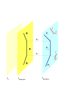
Figure 1: A schematic picture of the holographic dual description of DIS in the $1/\sqrt{\lambda}\ll x<1$ regime. $B$ denotes vector mesons, $r$ is the radial coordinate, $r_{0}$ is the IR cutoff, $r_{interaction}$ is where the graviton-meson interaction occurs (the position of the D7-brane), and $r_{Boundary}$ is where the actual field theory DIS process takes place. In this figure $l$ denotes leptons, dashed lines indicate virtual photons. This is a holographic dual representation of the forward Compton scattering, related to DIS through the optical theorem.

We have found several interesting results. On the one hand, we have obtained new relations among several of the eight different structure functions of each polarized vector meson. On the other hand, we have found that these relations are independent of the model: there could be a universal structure for holographic scalar and vector mesons. The reason for this behavior is the fact that the dynamics of holographic dual models with probe flavor Dp-branes is controlled by the Dirac-Born-Infeld (DBI) action. Although for each particular model the DBI action changes its dimension and also the structure of the gauge fields and the induced metric, it renders model-independent Callan-Gross type relations for different Dp-brane models when $1/\sqrt{\lambda}\ll x<1$, for instance $F_{2}=2F_{1}$. Notice though that for small-$x$ the Callan-Gross relation from QCD has an extra $x$-factor: $F_{2}=2xF_{1}$. Thus, it is expected that this additional factor should be present for small $x$ in the holographic dual description.

The next question is how to calculate the referred scalar and polarized vector meson structure functions at small and exponentially small values of $x$. This is the task we carry out in the present work. The calculations we perform hold in the planar limit of the gauge theory. Notice that for simplicity we restrict ourselves to the case of $N_{f}=1$, i.e. single-flavored mesons.

We address three main issues. As mentioned before, one is about the behavior of the structure functions at small and exponentially small $x$, in order to see if the rapid evolution towards small values of $x$ at strong coupling is confirmed for dynamical holographic mesons. Secondly, we show that for each holographic dual model we consider one may extract the Callan-Gross relation between $F_{1}$ and $F_{2}$, of the form $F_{2}\sim 2xF_{1}$, and similar additional relations among other structure functions. In fact as it happens with the glueballs [1] we find that there is also an extra $x$-independent (but model dependent) factor on the right hand side. Thirdly, we show how general these relations are, i.e. we discuss on their model-independent behavior. In order to carry out our programme we have to calculate the structure functions by using superstring theory. This has to be done in terms of the scattering amplitudes of two closed and two open strings. We will show the details in the following sections.

In Section 2 we study DIS of leptons by scalar mesons. Then, in Section 3 we carry out the calculation of the hadronic tensor of polarized vector mesons, including the structure functions and their relations at small values of the Bjorken parameter $x$ from string theory. We begin with the four-point scattering amplitudes of two open and two closed strings, ${\cal{A}}_{4}^{2o2c,scalar}$, in flat spacetime. This has two terms with two factors each: a kinematic one and a pre-factor which carries the $\alpha^{\prime}$-dependence. In the parametric regime we consider there is only one relevant term and from its kinematic factor one can obtain an effective four-point interaction Lagrangian. This Lagrangian describes an effective interaction between two gravitons and two scalar mesons. In the case of vector mesons the corresponding string theory scattering amplitude, ${\cal{A}}_{4}^{2o2c,vector}$, has several terms with two factors each: a kinematic one and a pre-factor. Again, we argue that there is only one relevant term and explain how one can obtain an effective four-point interaction Lagrangian. This Lagrangian describes an effective interaction between two gravitons and two polarized vector mesons. We should emphasize that this flat spacetime calculation is directly related to the scattering process in our curved background. This is so because in the small $x$ regime the size of the strings is small compared to the AdS curvature. As we shall see later this implies that the interaction can be considered local.

From the string theory scattering amplitude ${\cal{A}}_{4}^{2o2c}$ one can proceed in two different ways. In the first place, one can take the limit $\tilde{t}\rightarrow 0$, where $\tilde{t}$ is the ten-dimensional $t$-channel Mandelstam variable. From it one can obtain an effective Lagrangian, for which the relevant terms within the kinematic regime we describe consist of several four-point interaction vertices. Then, from this Lagrangian one can calculate the hadronic tensor for small and exponentially small values of $x$. There is a the second approach which we comment as follows. Let us consider the low-energy action of superstring theory, the Dp-brane action and the interaction between open and closed superstrings. Then, let us consider the $\alpha^{\prime}\rightarrow 0$ limit. From this low-energy theory we derive the graviton and meson propagators and also the interaction vertices. Then, we explicitly calculate the $s$-, $t$- and $u$-channels. It turns out that the coefficient of the $t$-channel graviton pole gives the same effective four-point interaction Lagrangian mentioned above up to an $\alpha^{\prime}$-dependent factor. A schematic representation of this process is depicted in figure 2. We carry out this calculation in full detail, and discuss its connection with the string theory four-point scattering amplitude.

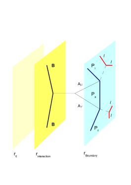
Figure 2: Schematic picture of the holographic dual description of DIS in the $\exp\left(-\sqrt{\lambda}\right)\ll x\ll 1/\sqrt{\lambda}$ regime. Here the graviton exchanged between the three-graviton vertex and the meson-meson-graviton vertex represents a single Pomeron exchange in the dual gauge theory.

Then, from these effective Lagrangians we derive the hadronic tensors of different mesons. Finally, we calculate the structure functions for scalar and polarized vector mesons. Particularly, for polarized vector mesons we obtain the alluded eight structure functions at small and exponentially small $x$ values. Very interestingly, we obtain new relations of the Callan-Gross type for several structure functions. These relations have similarities for all Dp-brane models we consider. This suggests a universal behavior which would possibly hold in the large $N$ limit of QCD.

In Sections 2 and 3 we carry out all the mentioned calculations for the specific case of the D3D7-brane model. We also comment on the exponentially small $x$ regime. In Section 4 we extend all these results, expressing them in a compact general form which also holds for the D4D6$\mathrm{\overline{D6}}$-brane model and for the D4D8$\mathrm{\overline{D8}}$-brane model. Discussions and conclusions are presented in Section 5.

2 DIS from scalar mesons at small $x$ from string theory

Let us consider the four-momentum of the hadron $P^{\mu}$, and the virtual photon four-momentum $q^{\mu}$, where $q^{2}>0$. Recall that the $s$-channel Mandelstam variable in the four-dimensional gauge theory is given by

$$s=-(P+q)^{2}=q^{2}\left(\frac{1}{x}-1-t_{B}\right)\simeq q^{2}\left(\frac{1}{x}-1\right)\,,$$ (2.1)

where we have considered the situation where $|P^{2}|\ll q^{2}$ (i.e. $|t_{B}|\ll 1$).

Since the gauge theory under consideration has a known string theory dual description, we will describe the deep inelastic scattering of an electron from a scalar meson with one flavor in terms of its holographic dual D3D7-brane model. The ten-dimensional background metric is

$$ds^{2}=\frac{r^{2}}{R^{2}}\,\eta_{\mu\nu}\,dx^{\mu}dx^{\nu}+\frac{R^{2}}{r^{2}}\,dr^{2}+R^{2}\,d\Omega_{5}^{2}\,,$$ (2.2)

where the radius of the five-sphere and the scale of the AdS₅ satifies $R^{4}=4\pi g_{c}N\alpha^{\prime 2}$. The usual four-dimensional coordinates are $x^{\mu}=(x^{0},\ldots,x^{3})$. The induced metric on the probe D7-brane is given by

$$ds^{2}_{D7}=\frac{r^{2}}{R^{2}}\,\eta_{\mu\nu}\,dx^{\mu}dx^{\nu}+\frac{R^{2}}{r^{2}}\,dr^{2}+R^{2}\,d\Omega^{2}_{3}\,,$$ (2.3)

which is the asymptotic form of the metric when $r$ is much larger than the distance between the D7-brane and the $N$ D3-branes. Scalar and vector mesons correspond to excitations of open strings ending on the probe D7-brane. The dynamics of the D7-brane fluctuations is described by the DBI action

$$S_{D7} = -T_{7}\int d^{8}\xi\,\sqrt{-\textmd{det}(\hat{P}[g]_{ab}+2\pi\alpha^{\prime}F_{ab})}\,,$$ (2.4)

where $g_{ab}$ stands for the metric (2.3), $T_{7}$ is the D7-brane tension. In addition, $\hat{P}$ denotes the pullback of the background fields on the D7-brane world-volume.

The ten-dimensional $s$-channel Mandelstam variable satisfies

$$\tilde{s}\leq-g^{\mu\nu}(P+q)_{\mu}(P+q)_{\nu}=\frac{1}{\sqrt{4\pi g_{c}N\alpha^{\prime 2}}}\bigg{(}\frac{1}{x}-1\bigg{)}\,.$$ (2.5)

The hadronic tensor can be extracted from the calculation of the four-point correlation function of two photons and two scalar mesons. While in the supergravity calculation there is a sum over intermediate states [13, 14], when we focus on the string theory calculation there is an implicit sum which is obtained by considering the imaginary part of the forward four-point scattering amplitude.

In the dual string theory model photons are represented by gravitons, $h$, with polarizations $h^{MN}=(1/2)(A^{M}v^{N}+A^{N}v^{M})$ where $A^{m}$ is a $U(1)$ gauge field propagating along $0,\dots,4$ coordinates in the bulk. For the D3D7-brane model $v^{i}$ is a constant Killing vector on the three-sphere. In superstring theory gravitons correspond to closed strings. On the other hand, scalar mesons are represented by open strings attached to the flavor D7-brane. Then, one has to calculate the four-point string theory scattering amplitude of two open and two closed strings, ${\cal{A}}_{4}^{2o2c,scalar}$. As mentiones before, this amplitude can be expressed in terms of two terms with two factors each. One is a kinematic factor, ${\cal{K}}_{i}^{2o2c,scalar}$. The other one is a pre-factor ${\cal{P}}_{i}^{2o2c,scalar}$ which has the usual gamma function structure, and it gives the $\alpha^{\prime}$-dependence:

$${\cal{A}}_{4}^{2o2c,scalar}={\cal{P}}_{1}^{2o2c,scalar}\,{\cal{K}}_{1}^{2o2c,scalar}+{\cal{P}}_{2}^{2o2c,scalar}\,{\cal{K}}_{2}^{2o2c,scalar}\,.$$ (2.6)

Within the kinematic regime we are interested in the second term is not relevant. We focus on the first term because this is the only one having a pole in the $t$-channel [18].

Since we are interested in the hadronic tensor, we want to calculate the imaginary part of the forward scattering amplitude. Essentially, we must evaluate ${\cal{K}}_{1}^{2o2c,scalar}$ at $\tilde{t}=0$. This can be done in two ways. On the one hand, we can take ${\cal{A}}_{4}^{2o2c,scalar}$ and replace $h^{mi}$ (the graviton, i.e. a closed string) by $A^{m}v^{i}$, and also consider $X$ which is the scalar fluctuation represented by an open string. Thus, in principle, one obtains an effective four-point interaction Lagrangian ${\cal{L}}_{hhXX}^{eff}$ from which the hadronic tensor can be calculated. On the other hand, ${\cal{L}}_{hhXX}^{eff}$ is also given by the coefficient of the $t$-channel graviton pole multiplied by a pre-factor with the $\alpha^{\prime}$-dependence. This second approach can be thought of as the low-energy calculation of the four-point scattering amplitude, i.e. in the $\alpha^{\prime}\rightarrow 0$ limit. For this calculation one considers the graviton propagator and the graviton three-point vertex derived from type IIB supergravity action, and also the graviton-$XX$ vertex derived from the Dirac-Born-Infeld action with scalar fluctuations on the flavor brane.

Notice that in what follows the momenta $k_{a}$ of the fields, the graviton polarizations $h$, and the polarization of the vector mesons $\epsilon$ (in Section 3) are parallel to the flavor D7-brane directions. On the other hand, the scalar mesons represent fluctuations perpendicular to the flavor D7-brane world-volume coordinates.

2.1 Four-point open-closed string theory amplitude

In order to obtain the tree-level scattering amplitude of two closed strings representing two gravitons, and two open strings which represent two scalar (or vector) mesons, we have to carry out a path integral with the corresponding vertex operator insertions on the world-sheet. In this case the world-sheet is a disk. In [18] it has been shown how any amplitude of open and closed strings can be mapped to pure open string amplitudes. This implies that disk amplitudes, which involve fields in the gauge multiplets and fields in the supergravity multiplet, are related to pure amplitudes involving only members from the gauge multiplets. The world-sheet tree-level diagram of an $S$-matrix for the open-closed string theory interaction can be conformally mapped to a surface with one boundary. Then, following the Riemann mapping theorem this surface is equivalent to the unit disk $\textbf{D}=\{z\in\textbf{C}|,|z|\leq 1\}$. By using the Möbius transformation $z\rightarrow i(1+z)(1-z)^{-1}$ this disk can be conformally mapped on the upper (complex) half-plane $\textbf{H}_{+}=\{z\in\textbf{C}|,\textmd{Im}(z)\geq 0\}$. Then, vertex operators create the string states corresponding to asymptotic states in the string theory $S$-matrix formulation. Since in theories with Dp-branes massless fields correspond to open string excitations on the Dp-brane world-volume, the disk tree-level diagram is attached to the Dp-brane world-volume. For closed string excitations, on the other hand, they propagate in the bulk of the ten-dimensional spacetime and they are inserted in the interior of the disk D. Thus, the open string vertex operators $V_{o}(x_{i})$ are inserted at the positions $x_{i}$ on the boundary of D, where $x_{i}$ is a real parameter. On the other hand, the closed string vertex operators $V_{c}({\bar{z}_{i}},z_{i})$ are inserted at the positions $z_{i}$ inside the disk D. The open string theory vertex operators are

$$V_{o}^{(-1)}(x,\epsilon_{\mu},p) = g_{o}e^{-\phi}\epsilon_{\mu}\psi^{\mu}e^{ip\cdot X}(x)\,,$$ (2.7)

$$V_{o}^{(0)}(x,\epsilon_{\mu},p) = g_{o}(2\alpha^{\prime})^{-1/2}\epsilon_{\mu}\left(i\partial_{x}X^{\mu}+2\alpha^{\prime}p\cdot\psi\psi^{\mu}\right)e^{ip\cdot X}(x)\,,$$ (2.8)

while for closed strings we have

$$V_{c}^{(-1,-1)}(z,\bar{z};h_{\mu\nu},q) = g_{c}e^{-\widetilde{\phi}(\bar{z})}e^{-\phi(z)}h_{\mu\nu}\widetilde{\psi}^{\mu}(\bar{z})\psi^{\nu}(z)e^{iq\cdot X(\bar{z},z)}\,,$$ (2.9)

$$V_{c}^{(0,0)}(z,\bar{z};h_{\mu\nu},p) = -g_{c}\frac{2}{\alpha^{\prime}}h_{\mu\nu}\left(i\bar{\partial}X^{\mu}+\frac{\alpha^{\prime}}{2}q\cdot\widetilde{\psi}\widetilde{\psi}^{\mu}(\bar{z})\right)\left(i\partial X^{\nu}+\frac{\alpha^{\prime}}{2}q\cdot\psi\psi^{\nu}(z)\right)$$ (2.10)

$$e^{iq\cdot X(\bar{z},z)}\,.$$

In the present notation $X^{\mu}$ and $\psi^{\mu}$ are the bosonic and fermionic fields on the world-sheet, while $\phi$ and $\widetilde{\phi}$ are the ghost fields which come from the Fadeev-Popov quantization of superstring theory. The open and closed string couplings are $g_{o}$ and $g_{c}$, respectively, with $g_{c}=g_{o}^{2}$.

Using these conventions the string theory scattering amplitude corresponding to two open strings, which are associated with excitation modes of a flavor Dp-brane, and two closed strings, which correspond to fields in the bulk, is given by the integral (2.1) over the disk. If we were interested in $1/N$ corrections, the corresponding corrections to the tree-level string theory scattering amplitudes would be given by the integrals over different inequivalent topologies. In addition, in the scattering amplitude we have to include the normal ordering of each vertex operator. Thus, in what follows whenever we write $V$ we mean $:V:$

$$A_{string}(h_{1},h_{4},\epsilon_{2},\epsilon_{3})=\int_{\bf{\partial H}_{+}}dx\int_{\bf{\partial H}_{+}}dy\int_{z\in\bf{H}_{+}}dzd\bar{z}\int_{w\in\bf{H}_{+}}dwd\bar{w}\,\langle c(z)\widetilde{c}(\bar{z})\times$$

$$V_{c}^{(0,0)}(z,\bar{z};h_{1\mu\nu},k_{1})V_{c}^{(-1,-1)}(w,\bar{w};h_{4\mu\nu},p_{4})(c(x)-c(y))V_{o}^{(0)}(x,\epsilon_{2\mu},k_{2})V_{o}^{(0)}(y,\epsilon_{3\mu},k_{3})\rangle,$$

where $c$ and $\tilde{c}$ are ghost fields. There are two real parameters associated with the insertions of the open string vertex operators and two complex parameters corresponding to the insertions of two closed string vertex operators. The world-sheet $SL(2,R)$ symmetry group allows us to fix three real parameters. Therefore, the number of integrals reduces to just three. Thus, a possibility is to set $x\rightarrow-\infty$, $y=1$ and $Re(w)=0$ (i.e. $\bar{w}=-w$). In addition, let us briefly comment on the vacuum expectation value in Eq.(2.1), which corresponds to a path integral over the fields on the world-sheet which we schematically represent as $\Phi\equiv\{X,\psi,\widetilde{\psi},\phi,\widetilde{\phi},c,\widetilde{c}\}$. Then, we have

$$\langle f[X,\psi,\widetilde{\psi},\phi,\widetilde{\phi},c,\widetilde{c}]\rangle\equiv\int D\Phi\ \ e^{iS[\Phi]}f[\Phi]\,,$$ (2.12)

which can be factorized as follows

$$S[\Phi]=S[X,\psi,\widetilde{\psi},\phi,\widetilde{\phi},c,\widetilde{c}]=S_{X}[X]+S_{\psi}[\psi,\widetilde{\psi}]+S_{\phi}[\phi,\widetilde{\phi}]+S_{c}[c,\widetilde{c}]\,.$$ (2.13)

This implies that each path integral can be done separately. Thus, in order to calculate the scattering amplitude (2.1) we can use the following expectation values of the fields [18, 19, 20]

$$\langle X^{\mu}(z)X^{\nu}(w)\rangle = -2\alpha^{\prime}\eta^{\mu\nu}\ln(z-w),$$

$$\langle X^{\mu}(z)\widetilde{X}^{\nu}(\bar{w})\rangle = -2\alpha^{\prime}D^{\mu\nu}\ln(z-\bar{w}),$$

$$\langle\psi^{\mu}(z)\psi^{\nu}(w)\rangle = \eta^{\mu\nu}(z-w)^{-1},$$

$$\langle\psi^{\mu}(z)\widetilde{\psi}^{\nu}(\bar{w})\rangle = D^{\mu\nu}(z-\bar{w})^{-1},$$

$$\langle\phi(z)\phi(w)\rangle = -\ln(z-w),$$

$$\langle\phi(z)\widetilde{\phi}(\bar{w})\rangle = -\ln(z-\bar{w}),$$

$$\langle c(w_{1})c(w_{2})c(z)\rangle = C_{ghost}(w_{1}-w_{2})(w_{1}-z)(w_{2}-z),$$

$$\langle c(w_{1})c(w_{2})\widetilde{c}(\bar{z})\rangle = C_{ghost}(w_{1}-w_{2})(w_{1}-\bar{z})(w_{2}-\bar{z}),$$

where $D^{\mu\nu}$ is a diagonal matrix whose elements are $1$ in the directions parallel to the flavor Dp-brane and $-1$ in the perpendicular directions. Thus, we have all the ingredients to calculate the expectation value in (2.1)

$$\langle c(z)\widetilde{c}(\bar{z})(c(x)-c(y))\rangle\langle e^{-\widetilde{\phi}(\bar{z})}e^{-\phi(z)}\rangle g_{c}^{2}\frac{2}{\alpha^{\prime}}\,g_{o}^{2}\frac{1}{2\alpha^{\prime}}h_{1\mu\nu}h_{4\rho\sigma}\epsilon_{2\alpha}\epsilon_{3\beta}\times$$

$$\langle\widetilde{\psi}^{\mu}(\bar{z})\psi^{\nu}(z)e^{ik_{1}\cdot X(\bar{z},z)}\left(i\bar{\partial}X^{\rho}+\frac{\alpha^{\prime}}{2}k_{4}\cdot\widetilde{\psi}\widetilde{\psi}^{\rho}(\bar{w})\right)\left(i\partial X^{\sigma}+\frac{\alpha^{\prime}}{2}k_{4}\cdot\psi\psi^{\sigma}(w)\right)e^{ik_{4}\cdot X(\bar{w},w)}$$

$$\left(i\partial_{x}X^{\alpha}+2\alpha^{\prime}k_{2}\cdot\psi\psi^{\alpha}\right)e^{ik_{2}\cdot X}(x)\left(i\partial_{y}X^{\beta}+2\alpha^{\prime}k_{3}\cdot\psi\psi^{\beta}\right)e^{ik_{3}\cdot X}(y)\rangle.$$ (2.14)

We have to obtain all the Wick’s contractions for 16 different terms. An important simplification comes from the fact that the contraction of two fields at the same point on the disk vanishes. The calculation is rather complicated but in the case of scalar mesons there is only one non-vanishing term. This is due to the fact that its corresponding polarizations (which are non-vanishing only in the perpendicular directions to the Dp-brane) are themselves perpendicular to all momenta as well as to all the rest of the polarizations of the fields. An early result was obtained by Fotopoulos and Tseytlin in [20] within the regime where superstring theory can be described by supergravity. In this case the integral was carried out close to the singularities. We perform similar calculations in the following section. More recently, in an extensive work Stieberger obtained the exact result [18], which can be split into two terms as anticipated in Eq.(2.6), where

$${\cal{P}}_{1}^{2o2c,scalar} = \int_{-\infty}^{+\infty}dx\,x^{2}(1+ix)^{u-1}(1-ix)^{u-1}\times$$

$$\int_{\mathbb{C}}d^{2}z\,(1-z)^{s}(1-\bar{z})^{s}(z+ix)^{\frac{t}{2}-1}(z-ix)^{\frac{t}{2}-1}(\bar{z}+ix)^{\frac{t}{2}-1}(\bar{z}-ix)^{\frac{t}{2}-1},$$

while ${\cal{K}}_{1}^{2o2c,scalar}$ can be obtained as the sum of the scattering amplitudes associted with the different Feynman diagrams from the supergravity calculation [20]. We only write the first term because in the kinematic regime which we are interested in only this term is relevant.

The pre-factor needed in order to construct the effective action of two closed-two open strings interaction is formally given by the small $\tilde{t}$ and large $\tilde{s}$ limit of expression (2.1). However, since it is rather difficult to deal with we will give several arguments to support the assumption that, in the scalar case, this pre-factor takes the same form that it has in the case of glueballs, i.e.

$$\frac{\pi\alpha^{\prime}}{4}\sum_{m=0}^{\infty}\delta\left(m-\frac{\alpha^{\prime}\tilde{s}}{4}\right)(m)^{\alpha^{\prime}\tilde{t}/4},$$ (2.16)

where we have omitted the $1/\tilde{t}$ term which leads to the $t$-channel as the dominant contribution and focused on the imaginary part that singles out the exchange of excited strings [1]. In [21] it has been shown that in this parameter regime the $\tilde{s}$-dependence always gives a factor

$$\left(\frac{\alpha^{\prime}\tilde{s}}{4}\right)^{\alpha^{\prime}\tilde{t}/4}=\int_{0}^{\infty}dm\,\delta\left(m-\frac{\alpha^{\prime}\tilde{s}}{4}\right)(m)^{\alpha^{\prime}\tilde{t}/4}\approx\sum_{m=1}^{\infty}\delta\left(m-\frac{\alpha^{\prime}\tilde{s}}{4}\right)(m)^{\alpha^{\prime}\tilde{t}/4}.$$ (2.17)

In the last step we have considered the fact that when $x\ll 1/\sqrt{\lambda}$ the integral and the sum are not very different. Note that in the small $x$ regime the factor $(m)^{\alpha^{\prime}\tilde{t}/4}$ is order one [1]. This approximation breaks down in the exponentially small regime. There is also a factor carrying the pole in $\tilde{t}$. In fact, the OPE expansion of the operators involved in this process have been studied both for a pair of closed superstrings [21] and for open superstrings [22, 23]. In both cases it is shown that this function gives a factor of the form

$$\frac{\Gamma\left(-1-\frac{\alpha^{\prime}\tilde{t}}{4}\right)}{\Gamma\left(2+\frac{\alpha^{\prime}\tilde{t}}{4}\right)}e^{i\pi(1-\alpha^{\prime}t/4)}\propto-\frac{1}{\alpha^{\prime}\tilde{t}}+O(1),$$ (2.18)

where the last result comes from the small $\tilde{t}$ expansion. Therefore, this supports the fact that we can neglect other possible terms in ${\cal{A}}_{4}^{2o2c,scalar}$ and ${\cal{A}}_{4}^{2o2c,vector}$, besides the one which does not vanish in the $\alpha^{\prime}\rightarrow 0$ limit. In addition, the OPE analysis also singles out the term where the polarizations of incoming gravitons and mesons ($h$ and $\epsilon$) are contracted among themselves as follows: $(h_{1}h_{4})(\epsilon_{2}\epsilon_{3})$. As we will see, this is in complete agreement with our calculations.

Finally, the assumption about the pre-factor is also supported a posteriori by our results: as will be demonstrated in the following sections, the kinematic part of the effective Lagrangian in the scalar meson case is identical to the one of [1] for glueballs. In addition, we have seen that from the string theory point of view the initial vertex operator integral, which leads to the full scattering amplitude at genus zero, is the same for scalar and vector mesons. This is because the only difference is given by the polarization vectors. This fact suggests the use of the same pre-factor as for the case of glueballs.

2.2 Four-point graviton-scalar meson tree-level amplitudes from supergravity

Schannel2 (40,25) i1,i2 o1,o2 dashesi1,v1 photoni2,v1 dashesv2,o1 photonv2,o2 dashesv1,v2 v1,v2 $h_{1}$i2 $h_{4}$o2 $X_{2}$i1 $X_{3}$o1 style_def marrowupa expr p = drawarrow subpath (1/4, 3/4) of p shifted 9 up withpen pencircle scaled 0.4; label.top(btex $k_{1}$ etex, point 0.7 of p shifted 15 up); enddef; marrowupa,tension=0i2,v1 style_def marrowupb expr p = drawarrow subpath (1/4, 3/4) of p shifted 9 down withpen pencircle scaled 0.4; label.bot(btex $k_{2}$ etex, point 0.7 of p shifted 15 down); enddef; marrowupb,tension=0i1,v1 style_def marrowupd expr p = drawarrow subpath (1/4, 3/4) of p shifted 9 up withpen pencircle scaled 0.4; label.top(btex $k_{4}$ etex, point 0.7 of p shifted 15 up); enddef; marrowupd,tension=0o2,v2 style_def marrowupe expr p = drawarrow subpath (1/4, 3/4) of p shifted 9 down withpen pencircle scaled 0.4; label.bot(btex $k_{3}$ etex, point 0.7 of p shifted 15 down); enddef; marrowupe,tension=0o1,v2       Uchannel2 (40,25) i1,i2 o1,o2 phantomi2,v1 phantomv2,o2 dashesv1,i1 dashesv2,o1 dashesv1,v2 photon,tension=0v1,o2 photon,tension=0v2,i2 v1,v2 $h_{1}$i2 $h_{4}$o2 $X_{2}$i1 $X_{3}$o1 style_def marrowshorta expr p = drawarrow subpath (1/4, 2/4) of p shifted 6 up withpen pencircle scaled 0.4; label.top(btex $k_{1}$ etex, point 0.4 of p shifted 7 up); enddef; marrowshorta,tension=0i2,v2 style_def marrowupb expr p = drawarrow subpath (1/4, 3/4) of p shifted 9 down withpen pencircle scaled 0.4; label.bot(btex $k_{2}$ etex, point 0.7 of p shifted 15 down); enddef; marrowupb,tension=0i1,v1 style_def marrowshortd expr p = drawarrow subpath (1/4, 2/4) of p shifted 6 up withpen pencircle scaled 0.4; label.top(btex $k_{4}$ etex, point 0.4 of p shifted 7 up); enddef; marrowshortd,tension=0o2,v1 style_def marrowupe expr p = drawarrow subpath (1/4, 3/4) of p shifted 9 down withpen pencircle scaled 0.4; label.bot(btex $k_{3}$ etex, point 0.7 of p shifted 15 down); enddef; marrowupe,tension=0o1,v2

Tchannel2 (40,25) i1,i2 o1,o2 photoni2,v1,o2 dashesi1,v2,o1 photonv1,v2 v1,v2 $h_{1}$i2 $h_{4}$o2 $X_{2}$i1 $X_{3}$o1 style_def marrowa expr p = drawarrow subpath (1/4, 3/4) of p shifted 6 up withpen pencircle scaled 0.4; label.top(btex $k_{1}$ etex, point 0.5 of p shifted 6 up); enddef; marrowa,tension=0i2,v1 style_def marrowb expr p = drawarrow subpath (1/4, 3/4) of p shifted 6 up withpen pencircle scaled 0.4; label.top(btex $k_{4}$ etex, point 0.5 of p shifted 6 up); enddef; marrowb,tension=0o2,v1 style_def marrowd expr p = drawarrow subpath (1/4, 3/4) of p shifted 6 down withpen pencircle scaled 0.4; label.bot(btex $k_{3}$ etex, point 0.5 of p shifted 6 down); enddef; marrowd,tension=0o1,v2 style_def marrowe expr p = drawarrow subpath (1/4, 3/4) of p shifted 6 down withpen pencircle scaled 0.4; label.bot(btex $k_{2}$ etex, point 0.5 of p shifted 6 down); enddef; marrowe,tension=0i1,v2       Contact2 (40,25) i1,i2 o1,o2 photoni2,v1,o2 dashesi1,v1,o1 v1 $h_{1}$i2 $h_{4}$o2 $X_{2}$i1 $X_{3}$o1 style_def marrowupa expr p = drawarrow subpath (1/4, 3/4) of p shifted 9 up withpen pencircle scaled 0.4; label.top(btex $k_{1}$ etex, point 0.7 of p shifted 15 up); enddef; marrowupa,tension=0i2,v1 style_def marrowupb expr p = drawarrow subpath (1/4, 3/4) of p shifted 9 up withpen pencircle scaled 0.4; label.top(btex $k_{4}$ etex, point 0.7 of p shifted 15 up); enddef; marrowupb,tension=0o2,v1 style_def marrowupd expr p = drawarrow subpath (1/4, 3/4) of p shifted 9 down withpen pencircle scaled 0.4; label.bot(btex $k_{3}$ etex, point 0.7 of p shifted 15 down); enddef; marrowupd,tension=0o1,v1 style_def marrowupe expr p = drawarrow subpath (1/4, 3/4) of p shifted 9 down withpen pencircle scaled 0.4; label.bot(btex $k_{2}$ etex, point 0.7 of p shifted 15 down); enddef; marrowupe,tension=0i1,v1

Figure 3: The four Feynman diagrams corresponding to the holographic calculation of the four-point amplitude: $s$-, $u$-, and $t$-channels plus the contact interaction. Wavy lines represent gravitons, $h_{1}$, $h_{4}$ and the off-shell one. Dashed lines represent scalar mesons, $X_{2}$ and $X_{3}$. $k_{i}$ indicates the momenta of the fields.

We begin with the action

$$S_{DBI}=-T_{7}\int d^{8}\xi\sqrt{-det\left(\hat{P}[g]_{ab}+(2\pi\alpha^{\prime})F_{ab}\right)}\,,$$ (2.19)

and

$$\sqrt{-g}\approx\sqrt{-g_{0}}\left[1+\frac{1}{2}H-\frac{1}{4}H^{a}_{b}H^{b}_{a}+\frac{1}{8}H^{2}+\frac{1}{6}H^{a}_{b}H^{b}_{c}H^{c}_{a}-\frac{1}{8}HH^{a}_{b}H^{b}_{a}+\frac{1}{48}H^{3}\right]\,,$$ (2.20)

where $H\equiv H^{a}_{a}$ stands for trace of this tensor field. There are eight coordinates which are parallel to the D7-brane, and two perpendicular ones, $x^{8}$ and $x^{9}$. We can describe the degrees of freedom of the system by identifying $\xi^{a}\equiv X^{a}$ with $a=0,\dots,7$ and reinterpreting the $(8,9)$-coordinates as scalar fields $X^{I}$ with $I=1,2$. Their variation parametrize fluctuations of the D7-brane along its normal directions. By using this static parametrization, and by ignoring all vector fields $F_{ab}$, we identify the fields in our theory with the metric perturbations associated with the graviton and the scalar fields as follows

$$H_{ab}\rightarrow\hat{g}_{ab}\equiv g_{ab}+2g_{I(a}\partial_{b)}X^{I}+g_{IJ}\,\partial_{a}X^{I}\partial_{b}X^{J},$$ (2.21)

$$g_{ab}=\eta_{ab}+2\kappa h_{ab}\ ,\ g_{IJ}=\delta_{IJ}+2\kappa h_{IJ}\ ,\ g_{aI}=2\kappa h_{aI}.$$ (2.22)

Now, we will focus on the case where the graviton polarization is parallel to the D7-brane, which implies that $h_{IJ}=h_{aI}=0$. By expanding $S_{DBI}$, we obtain three of the necessary ingredients for the calculation of the tree-level Feynman diagrams. These diagrams are analogous to those obtained in the low-energy limit of a closed string theory, when considering graviton-dilaton interactions, namely: the kinetic term associated with the scalar fields and the interactions of the type $hXX$ and $hhXX$. Notice that since the scalar term in $H$ is quadratic, we only need to do the expansion up to third order. Also recall that the three-graviton vertex and the graviton propagator come directly from the closed string theory action [24, 25, 20] .

The first order in the expansion above gives a kinetic term $\frac{T_{7}}{2}\partial_{a}X\partial^{a}X$ . Therefore, the propagator is

$$P_{IJ}(k)\equiv\langle X_{I}X_{J}\rangle=-i\frac{\delta_{IJ}}{T_{7}k^{2}}.$$ (2.23)

The second and third orders in the expansion produce the following interaction Lagrangians

$$L_{hXX} = T_{7}\kappa\left[\frac{1}{2}h\partial^{a}X\partial_{a}X-h^{a}_{b}\partial^{b}X\partial_{a}X\right],$$ (2.24)

$$L_{hhXX} = T_{7}\kappa^{2}\left[\frac{1}{4}h^{2}\partial^{a}X\partial_{a}X+2h^{a}_{b}h^{b}_{c}\partial^{c}X\partial_{a}X-hh^{a}_{b}\partial^{b}X\partial_{a}X-\frac{1}{2}h^{a}_{b}h^{b}_{a}\partial^{c}X\partial_{c}X\right],$$

where $h=h_{a}^{a}$. Notice that for the contact term $V_{hhXX}$ we can ignore terms with a factor $h^{a}_{a}$ since the external gravitons are on-shell and therefore traceless. However, this does not hold for the $V_{hXX}$ vertex since in the $t$-channel diagram this vertex exchanges a virtual graviton with the three-graviton vertex. Let us call $k_{1}$ and $k_{2}$ the incoming momenta of the scalar field, then we obtain

$$V_{hXX}^{ab,IJ} = iT_{7}\kappa\,\delta^{IJ}\left[\frac{1}{2}\eta^{ab}(k_{1}\cdot k_{2})-(k_{1}^{a}k_{2}^{b}+k_{1}^{b}k_{2}^{a})+\text{irrelevant}\right]\,$$ (2.26)

$$V_{hhXX}^{ab,cd,IJ}(k_{1},k_{2}) = 4iT_{7}\kappa^{2}\,\delta^{IJ}\left[\eta^{bc}(k_{1}^{a}k_{2}^{d}+k_{1}^{d}k_{2}^{a})-\frac{1}{2}\eta^{ac}\eta^{bd}(k_{1}\cdot k_{2})\right]\,.$$ (2.27)

For instance, the scattering amplitude related to the contact diagram (subindex $c$ indicates contact term) is given by

$$A_{c}(k_{1},k_{2},k_{3},k_{4}) = h_{1ab}\,h_{4de}\,\delta_{IJ}\,V_{hhXX}^{ab,de,IJ}(k_{2},k_{3})$$ (2.28)

$$= i\kappa^{2}T_{7}\left[4(k_{2}h_{1}h_{4}k_{3})+4(k_{3}h_{1}h_{4}k_{2})-2(h_{1}h_{4})(k_{2}\cdot k_{3})\right],$$

where indices of factors within parentheses are totally contracted. In addition, in order to calculate the scattering amplitudes corresponding to the $s$- and $u$-channels from the previous vertices, and by using the transversal character of the polarizations, momentum conservation and the dispersion relations for massless particles, we obtain the following results

$$A_{s}(k_{1},k_{2},k_{3},k_{4}) = h_{1ab}\,h_{4cd}\,\delta_{IJ}\,V_{hXX}^{ab,IK}(k_{2},-k_{1}-k_{2})P_{KL}(-k_{1}-k_{2})V^{cd,LJ}(k_{1}+k_{2},k_{3})$$ (2.29)

$$= -i\kappa^{2}T_{7}\frac{4}{s}(k_{2}h_{1}k_{2})(k_{3}h_{4}k_{3})\,,$$

$$A_{u}(k_{1},k_{2},k_{3},k_{4}) = h_{1ab}\,h_{4cd}\,\delta_{IJ}\,V_{hXX}^{ab,JK}(k_{3},-k_{1}-k_{3})P_{KL}(-k_{1}-k_{3})V^{cd,LI}(k_{1}+k_{3},k_{2})$$ (2.30)

$$= -i\kappa^{2}T_{7}\frac{4}{u}(k_{3}h_{1}k_{3})(k_{2}h_{4}k_{2})\,,$$

where $s=-2k_{1}\cdot k_{2}=-2k_{3}\cdot k_{4}$ while $u=-2k_{1}\cdot k_{3}=-2k_{2}\cdot k_{4}$.

Now, let us consider the $t$-channel. We need three pieces: the three-graviton vertex derived from $L_{hhh}$, the graviton propagator which is derived from $L^{\partial^{2}}_{hh}$, and the three-point interaction vertex with one graviton and two scalars derived from $L_{hXX}$ which we have already obtained. The graviton that connects the three-graviton vertex from $L_{hhh}$ and the interaction vertex $V_{hXX}$ is off-shell, and therefore we cannot neglect the first term. Also, note that since we will contract this vertex with the graviton propagator it is not necessary to symmetrize the vertex in the $\alpha$ and $\beta$ Lorentz indices. This vertex must then be contracted with a factor $S^{\rho\sigma,\gamma\delta,\alpha\beta}(k_{1},k_{4})$ obtained for example by Sannan [25], which corresponds to the contraction of the off-shell graviton propagator and the three-graviton vertex. We must also contract this factor with the polarizations of the external gravitons $h_{1}$ and $h_{4}$. The resulting factor is

$$h_{1\rho\sigma}h_{4\gamma\delta}S^{\rho\sigma,\gamma\delta,\alpha\beta}(k_{1},k_{4})=$$

$$-\kappa\left[\frac{1}{2}(h_{1}h_{4})^{\alpha\beta}+\frac{1}{2}(h_{1}h_{4})^{\beta\alpha}+\frac{1}{t}\left((k_{1}h_{4})^{\alpha}(k_{4}h_{1})^{\beta}+(k_{1}h_{4})^{\beta}(k_{4}h_{1})^{\alpha}\right)\right.$$

$$\left.-\frac{(h_{1}h_{4})}{t}\left(k_{1}^{\alpha}k_{1}^{\beta}+k_{4}^{\alpha}k_{4}^{\beta}+\frac{1}{2}k_{4}^{\alpha}k_{1}^{\beta}+\frac{1}{2}k_{1}^{\alpha}k_{4}^{\beta}\right)-\frac{1}{t}\left((k_{1}h_{4}k_{1})h_{1}^{\alpha\beta}+(k_{4}h_{1}k_{4})h_{4}^{\alpha\beta}\right)\right.$$

$$\left.+\frac{1}{t}\left((k_{1}h_{4}h_{1})^{\alpha}k_{1}^{\beta}+(k_{1}h_{4}h_{1})^{\beta}k_{1}^{\alpha}+(k_{4}h_{1}h_{4})^{\alpha}k_{4}^{\beta}+(k_{4}h_{1}h_{4})^{\beta}k_{4}^{\alpha}\right)\right].$$ (2.31)

As mentioned before we take $\alpha,\beta\rightarrow a,b$ and contract this result with the vertex $V_{hXX}^{ab,I,J}$, obtaining the $t$-channel amplitude for the process

$$A_{t}(k_{1},k_{2},k_{3},k_{4})=h_{1cd}h_{4ef}S^{cd,df,ab}(k_{1},k_{4})V_{hXX}^{ab,I,J}(k_{2},k_{3})\delta_{IJ}=$$

$$\frac{-2i\kappa^{2}T_{7}}{sut}\big{[}\frac{1}{4}(h_{1}h_{4})(t^{2}+u^{2}+s^{2})+u[(k_{3}h_{1}h_{4}k_{1})+(k_{4}h_{1}h_{4}k_{2})]$$ (2.32)

$$+s[(k_{2}h_{1}h_{4}k_{1})+(k_{4}h_{1}h_{4}k_{3})]+t[(k_{2}h_{1}h_{4}k_{3})+(k_{3}h_{1}h_{4}k_{2})-(k_{4}h_{1}h_{4}k_{1})]+$$

$$2\left[(k_{4}h_{1}k_{2})(k_{3}h_{4}k_{1})+(k_{4}h_{1}k_{3})(k_{2}h_{4}k_{1})-(k_{4}h_{1}k_{4})(k_{2}h_{4}k_{3})-(k_{2}h_{1}k_{3})(k_{1}h_{4}k_{1})\right]\big{]},$$

being $t=-2k_{1}\cdot k_{4}=-2k_{2}\cdot k_{3}$. Notice that $(su)^{-1}$ has been factorized for convenience, however the graviton pole of the $t$-channel does appear.

The total tree-level scattering amplitude associated with this process is $A_{total}=A_{c}+A_{s}+A_{u}+A_{t}$. As we shall see later, this structure coincides with the scattering amplitude of closed string theory with two gravitons and two dilatons up to a global factor $su$. This means that, since the Feynman diagrams are the same, $A_{total}$ reproduces the kinematic factor of the closed string theory four-point scattering amplitude obtained from the world-sheet integration of the expectation value of four string theory vertex operators described in the previous section. In fact, the four-point closed string scattering amplitude is a known result given by

$$A_{4}^{closed}=-i\pi^{2}g_{c}\alpha^{\prime 3}\frac{\Gamma\left(-\frac{\alpha^{\prime}s}{4}\right)\Gamma\left(-\frac{\alpha^{\prime}u}{4}\right)\Gamma\left(-\frac{\alpha^{\prime}t}{4}\right)}{\Gamma\left(1+\frac{\alpha^{\prime}s}{4}\right)\Gamma\left(1+\frac{\alpha^{\prime}u}{4}\right)\Gamma\left(1+\frac{\alpha^{\prime}t}{4}\right)}\times K_{4}^{closed}\,,$$ (2.33)

where the pre-factor is proportional to $(stu)^{-1}$ at first order in $\alpha^{\prime}$. On the other hand, $K_{4}^{closed}$ is a kinematic factor which contains the polarizations. This does not depend on $\alpha^{\prime}$ and can be separated into kinematic factors associated with open string theory scattering amplitudes as

$$K_{4}^{closed}(k_{1},k_{2},k_{3},k_{4})\propto K_{4}^{open}\left(\frac{1}{2}k_{1},\frac{1}{2}k_{2},\frac{1}{2}k_{3},\frac{1}{2}k_{4}\right)\times K_{4}^{open}\left(\frac{1}{2}k_{1},\frac{1}{2}k_{2},\frac{1}{2}k_{3},\frac{1}{2}k_{4}\right).$$ (2.34)

We can explicitly calculate the scattering amplitude from $K_{4}^{open}$ which can be found in [26], and replace the graviton polarizations as $h_{1}^{MN}$ and $h_{2}^{MN}$, using the transversality condition and the fact that on-shell gravitons are traceless. The dilatons’ polarizations are also transversal

$$\frac{1}{\sqrt{8}}\phi_{2}\left(\eta^{MN}-k_{2}^{M}\bar{k_{2}}^{N}-k_{2}^{N}\bar{k_{2}}^{M}\right)\ ,\ \frac{1}{\sqrt{8}}\phi_{3}\left(\eta^{MN}-k_{3}^{M}\bar{k_{3}}^{N}-k_{3}^{N}\bar{k_{3}}^{M}\right).$$

The auxiliary momenta $\bar{k_{2}}$ and $\bar{k_{3}}$ satisfy the following relations $\bar{k_{2}}\cdot\bar{k_{2}}=\bar{k_{3}}\cdot\bar{k_{3}}=0$ and $k_{2}\cdot\bar{k_{2}}=k_{3}\cdot\bar{k_{3}}=1$. The only reason to include them is in order to have transversal polarizations. Thus, although they are important within the intermediate steps in the explicit calculations they never appear in the final results. Therefore, it is said that these momenta decouple from any physical process.

Recall that we want to study string theory scattering amplitudes in a curved spacetime. It is then important to think of the validity of the calculations that we perform since we do it for the string theory scattering amplitudes in flat spacetime. In order to answer this question we may separate the fields of the conformal theory on the world-sheet from the interaction, by considering the zero modes separated from the excited modes, i.e. $X^{M}(\tau,\sigma)=x^{M}+\tilde{X}^{M}(\tau,\sigma)$. At a fixed point $x^{M}$, the Gaussian integral over the modes $\tilde{X}^{M}$ is exactly the same as the one we would have in flat spacetime rendering a local amplitude $iA_{local}(x^{M})$. Thus, if we integrate over the zero modes, i.e. in flat spacetime, we obtain an $S$-matrix of the form

$$S=i\int d^{10}x\,\sqrt{-g}\,A_{local}(x^{M}).$$ (2.35)

This is equivalent to say that the interaction is approximately local, and this holds because the scale $\alpha^{\prime}$ is small compared to the spacetime curvature. This local approximation breaks down when $x$ becomes exponentially small [21].

2.3 Effective Lagrangian with four-point interactions

The idea now is to obtain an effective action with four-point interactions involving two gravitons and two scalar mesons. Thus, we have to start from the four-point string theory scattering amplitude that we have discussed before. It is important to recall that since the Bjorken parameter is small in the DIS regime we consider, i.e. $t\approx 0$ is very small, the Mandelstam variables $u$ and $s$ become very large. On the one hand, it is necessary to perform appropriate approximations on the pre-factor which we will discuss later. On the other hand, we have to find the leading terms coming from the kinematic factor, which are those that produce the $t$-channel scattering amplitude in the supergravity approximation. Since we look for a four-point interaction Lagrangian we can start by writing a list of the terms which, a posteriori, will be necessary in order to reproduce the $t$-channel scattering amplitude at leading order in the $t\approx 0$ approximation. These are

$${\cal{L}}_{A} = \partial_{n}h_{mp}\partial^{n}h^{mp}\partial_{M}X\partial^{M}X\rightarrow(h_{1}h_{4})t^{2},$$

$${\cal{L}}_{B} = \partial^{m}h^{pr}\partial^{n}h_{pr}\partial_{m}X\partial_{n}X\rightarrow\frac{1}{2}(h_{1}h_{4})(s^{2}+u^{2}),$$

$${\cal{L}}_{C} = \partial_{m}h^{np}\partial_{n}h_{p}^{m}\partial_{M}X\partial^{M}X\rightarrow-2t(k_{4}k_{1}h_{4}k_{1}),$$

$${\cal{L}}_{D} = \partial^{m}h^{pr}\partial_{p}h_{r}^{n}\partial_{m}X\partial_{n}X\rightarrow-\frac{1}{2}s\left[(k_{4}h_{1}h_{4}k_{3})+(k_{2}h_{1}h_{4}k_{1})\right]$$

$$-\frac{1}{2}u\left[(k_{3}h_{1}h_{4}k_{1})+(k_{4}h_{1}h_{4}k_{2})\right],$$

$${\cal{L}}_{E} = \partial^{p}h^{mr}\partial_{p}h_{r}^{n}\partial_{m}X\partial_{n}X\rightarrow-t[(k_{2}h_{1}h_{4}k_{3})+(k_{3}h_{1}h_{4}k_{2})],$$

$${\cal{L}}_{F} = \partial_{p}h^{rm}\partial_{r}h^{pn}\partial_{m}X\partial_{n}X\rightarrow 2[(k_{2}h_{1}k_{4})(k_{3}h_{4}k_{1})+(k_{3}h_{1}k_{4})(k_{2}h_{4}k_{1})],$$

$${\cal{L}}_{G} = h^{rp}\partial_{r}\partial_{p}h^{mn}\partial_{m}X\partial_{n}X\rightarrow 2[(k_{1}h_{4}k_{1})(k_{2}h_{1}k_{3})+(k_{4}h_{1}k_{4})(k_{2}h_{4}k_{3})].$$ (2.36)

By comparison with the coefficient of the $t$-channel graviton pole we can write the following effective Lagrangian

$${\cal{L}}_{eff}\propto\frac{1}{4}\times{\cal{L}}_{A}+\frac{1}{2}\times{\cal{L}}_{B}+\frac{1}{2}\times{\cal{L}}_{C}-2\times{\cal{L}}_{D}-1\times{\cal{L}}_{E}+1\times{\cal{L}}_{F}-1\times{\cal{L}}_{G}.$$ (2.37)

There is also a global factor $su$ which, for convenience, we will include in the pre-factor. Now, the metric perturbation we consider is $h^{ab}\equiv\frac{1}{2}(A^{a}v^{b}+A^{b}v^{a})$, where $A^{m}$ is a $U(1)$ gauge field while $v^{i}$ is a constant Killing vector on $S^{3}$. Recall that the D7-brane wraps this sphere, therefore we can rewrite the effective Lagrangian using the following identities

$$\partial_{b}h_{ac}\partial^{b}h^{ac} = \frac{1}{2}v^{c}v_{c}\partial_{b}A_{a}\partial^{b}A^{a}\ ,\ \partial^{a}h^{cd}\partial^{b}h_{cd}=\frac{1}{2}v^{c}v_{c}\partial^{a}A_{d}\partial^{b}A^{d},$$

$$\partial_{c}h^{da}\partial_{d}h^{cb} = \frac{1}{4}v^{a}v^{b}\partial_{c}A^{d}\partial_{d}A^{c}\ ,\ \partial_{a}h^{bc}\partial_{b}h_{c}^{a}=\frac{1}{4}v^{c}v_{c}\partial_{a}A^{b}\partial_{b}A^{a},$$

$$\partial^{a}h^{cd}\partial_{c}h_{d}^{b} = \frac{1}{4}v^{d}v_{d}\partial^{a}A^{c}\partial_{c}A^{b}\ ,\ \partial^{c}h^{ad}\partial_{c}h_{d}^{b}=\frac{1}{4}(v^{d}v_{d}\partial^{c}A^{a}\partial_{c}A^{b}+v^{a}v^{b}\partial^{c}A^{d}\partial_{c}A_{d}).$$

Once a graviton polarization is chosen in this way the term ${\cal{L}}_{G}$ vanishes. By taking into account that the terms in the scattering amplitude which are proportional to $t$ are irrelevant in the present regime, we can write an explicitly gauge invariant effective Lagrangian for the gauge field $A^{m}$. Thus, we have

$${\cal{L}}_{eff}\propto\frac{1}{4}\left[2\,v^{i}v_{i}\,\partial_{m}X\partial^{p}X\,F^{mn}F_{pn}+v^{i}v^{j}\,\partial_{i}X\partial_{j}X\,F^{mn}F_{mn}\right]\,,$$ (2.38)

where $F_{mn}=\partial_{m}A_{n}-\partial_{n}A_{m}$. In this Lagrangian the most important term is the first one since it leads to terms proportional to $s^{2}$ and $s$ in the scattering amplitude. As we shall see in Section 3, there is an analogous effective Lagrangian for vector mesons.

Eff2 (45,30) path quadrant, q[], otimes; quadrant = (0, 0) – (0.5, 0) & quartercircle (0, 0.5) – (0, 0); for i=1 upto 4: q[i] = quadrant rotated (45 + 90*i); endfor otimes = q[1] q[2] q[3] q[4] – cycle; i1,i2 o1,o2 photoni2,v1,o2 dashesi1,v1,o1 d.sh=otimes,d.f=empty,d.si=.1wv1 $h_{1}$i2 $h_{4}$o2 $X_{2}$i1 $X_{3}$o1 style_def marrowupa expr p = drawarrow subpath (1/4, 3/4) of p shifted 9 up withpen pencircle scaled 0.4; label.top(btex $k_{1}$ etex, point 0.7 of p shifted 15 up); enddef; marrowupa,tension=0i2,v1 style_def marrowupb expr p = drawarrow subpath (1/4, 3/4) of p shifted 9 up withpen pencircle scaled 0.4; label.top(btex $k_{4}$ etex, point 0.7 of p shifted 15 up); enddef; marrowupb,tension=0o2,v1 style_def marrowupd expr p = drawarrow subpath (1/4, 3/4) of p shifted 9 down withpen pencircle scaled 0.4; label.bot(btex $k_{3}$ etex, point 0.7 of p shifted 15 down); enddef; marrowupd,tension=0o1,v1 style_def marrowupe expr p = drawarrow subpath (1/4, 3/4) of p shifted 9 down withpen pencircle scaled 0.4; label.bot(btex $k_{2}$ etex, point 0.7 of p shifted 15 down); enddef; marrowupe,tension=0i1,v1

Figure 4: Effective four-point interaction. Wavy lines represent on-shell gravitons. Dashed lines represent scalar mesons.

2.4 Hadronic tensor at small $x$ for scalar mesons

We can use the same approximation as in [1], namely: based on the the effective Lagrangian (2.38) we can construct an effective action in curved spacetime by contracting all indices with the ten-dimensional metric in curved spacetime and also by multiplying by the squared root of the determinant of that metric as usual. Therefore, we begin with

$$n^{*}_{\mu}n_{\nu}\text{Im}_{exc}T^{\mu\nu}=\frac{\pi\alpha^{\prime}}{8}\sum_{m=1}^{\infty}\int d\Omega_{3}\,dr\,\sqrt{-g}v_{i}v^{i}\partial^{k}X^{*}(P)\partial^{n}X(P)F_{kp}^{*}(q)F_{n}^{p}(q)\delta\left(m-\frac{\alpha^{\prime}\tilde{s}}{4}\right)\,.$$ (2.39)

We have omitted the integrals in the four-dimensional spacetime $x_{0},\cdot\cdot\cdot,x_{3}$ since we have already used momentum conservation. The solutions to the field equations are [13]

$$A_{\mu}(q) = n_{\mu}f(r)e^{iq\cdot x}\,,$$ (2.40)

$$A_{r}(q) = \frac{-iq\cdot n}{q^{2}}f^{\prime}(r)e^{iq\cdot x}\,,$$ (2.41)

$$X^{l} = \frac{c_{i}^{l}}{\Lambda R^{3}}\left(\frac{r}{\Lambda R^{2}}\right)^{-\Delta}Y^{l}(\Omega_{3})e^{iP\cdot x}\,,$$ (2.42)

where $\Delta$ stands for the scaling dimension of the meson fields and $c_{i}$ is a dimensionless constant. By using $\omega=qR^{2}/r$ we can write $f=\omega K_{1}(\omega)$, where $K_{1}$ is the modified Bessel function of the second kind. In order to simplify the notation we drop the label $l$ which is associated with the spherical harmonic. Recall that this index identifies each meson. The corresponding field strengths are

$$F_{\mu\nu} = i(q_{\mu}A_{\nu}-q_{\nu}A_{\mu})=i(q_{\mu}n_{\nu}-q_{\nu}n_{\mu})f(r)e^{iq\cdot x}\,,$$ (2.43)

$$F_{\mu r} = i\left(q_{\mu}-n_{\mu}\frac{q^{2}}{q\cdot n}\right)A_{r}=\left(\frac{q\cdot n}{q^{2}}q_{\mu}-n_{\mu}\right)f^{\prime}(r)e^{iq\cdot x}\,,$$ (2.44)

$$\partial_{\nu}X = iP_{\nu}X\,,\,\,\,\,\,\,\partial_{r}X=\frac{-\Delta}{r}X\,,$$ (2.45)

from which we can construct the different pieces involved in the effective Lagrangian

$$F_{rp}^{*}F_{r}^{p} = \frac{R^{2}}{r^{2}}\eta^{\rho\sigma}F_{r\rho}^{*}F_{r\sigma}=\frac{R^{2}}{r^{2}}(f^{\prime})^{2}\left[(n\cdot n^{*})-\frac{(q\cdot n)(q\cdot n^{*})}{q^{2}}\right]\,,$$ (2.46)

$$F_{rp}^{*}F_{\mu}^{p} = \frac{R^{2}}{r^{2}}\eta^{\rho\sigma}F_{r\rho}^{*}F_{\mu\sigma}=i\frac{R^{2}}{r^{2}}ff^{\prime}q_{\mu}\left[(n\cdot n^{*})-\frac{(q\cdot n)(q\cdot n^{*})}{q^{2}}\right]\,,$$ (2.47)

$$F_{\mu p}^{*}F_{\nu}^{p} = \frac{R^{2}}{r^{2}}\eta^{\rho\sigma}F_{\mu\rho}^{*}F_{\nu\sigma}+\frac{r^{2}}{R^{2}}F_{\mu r}^{*}F_{\nu r}$$

$$= \frac{R^{2}}{r^{2}}f^{2}\left[q_{\mu}q_{\nu}(n^{*}\cdot n)+n_{\mu}^{*}n_{\nu}q^{2}-q_{\mu}n_{\nu}(q\cdot n^{*})-q_{\nu}n_{\mu}^{*}(q\cdot n)\right]$$

$$+\frac{r^{2}}{R^{2}}(f^{\prime})^{2}\left[n_{\mu}^{*}n_{\nu}+q_{\mu}q_{\nu}\frac{(q\cdot n)(q\cdot n^{*})}{q^{4}}-q_{\mu}n_{\nu}\frac{(q\cdot n^{*})}{q^{2}}-q_{\nu}n_{\mu}^{*}\frac{(q\cdot n)}{q^{2}}\right]$$

$$= \left(n^{*}_{\mu}-q_{\mu}\frac{q\cdot n^{*}}{q^{2}}\right)\left(n_{\nu}-q_{\nu}\frac{q\cdot n}{q^{2}}\right)\frac{\omega^{4}}{R^{2}}[K^{2}_{0}(\omega)+K^{2}_{1}(\omega)]$$

$$+q_{\mu}q_{\nu}\left(n^{*}\cdot n-\frac{(q\cdot n)(q\cdot n^{*})}{q^{2}}\right)\frac{\omega^{4}}{q^{2}R^{2}}K^{2}_{1}(\omega)\,,$$

and

$$\partial^{r}X^{*}(P)\partial^{r}X(P) = \frac{r^{2}\Delta^{2}}{R^{4}}|X|^{2},\,\,\,\,\,\,\partial^{\mu}X^{*}(P)\partial^{r}X(P)=-\frac{i\Delta}{r}P^{\mu}|X|^{2},$$ (2.49)

$$\partial^{\mu}X^{*}(P)\partial^{\nu}X(P) = \frac{R^{4}}{r^{4}}P^{\mu}P^{\nu}|X|^{2}\,.$$ (2.50)

Now, since we want to calculate $T^{\mu\nu}$, and then to contract it with the leptonic tensor, all terms with factors $q\cdot n$ and/or $q\cdot n^{*}$ will vanish. Therefore, we only need to expand the effective Lagrangian in terms of the solutions of the fields. In this way we can express the effective four-point interaction Lagrangian as

$${\cal{L}}_{4}^{eff} = {\cal{L}}_{4,A}^{eff}+{\cal{L}}_{4,B}^{eff}+{\cal{L}}_{4,C}^{eff}+{\cal{L}}_{4,D}^{eff}\,,$$ (2.51)

where

$${\cal{L}}_{4,A}^{eff} = \partial^{r}X^{*}(P)\partial^{r}X(P)F_{rp}^{*}F_{r}^{p}=\frac{\Delta^{2}}{R^{2}}(f^{\prime})^{2}(n\cdot n^{*})|X|^{2}\,,$$

$${\cal{L}}_{4,B}^{eff} = \partial^{\mu}X^{*}(P)\partial^{r}X(P)F_{\mu p}^{*}F_{r}^{p}=\frac{R^{2}\Delta}{r^{3}}ff^{\prime}(n\cdot n^{*})|X|^{2}(P\cdot q)={\cal{L}}_{4,C}^{eff}\,,$$

$${\cal{L}}_{4,D}^{eff} = \partial^{\mu}X^{*}(P)\partial^{\nu}X(P)F_{\mu p}^{*}F_{\nu}^{p}=\frac{R^{4}|X|^{2}}{r^{4}}\times\left[\frac{R^{2}}{r^{2}}(n\cdot n^{*})f^{2}(P\cdot q)^{2}+\right.$$

$$\left.\left(\frac{R^{2}}{r^{2}}q^{2}f^{2}+\frac{r^{2}}{R^{2}}(f^{\prime})^{2}\right)(P\cdot n)(P\cdot n^{*})\right]\,.$$

It is worth noting that the terms ${\cal{L}}_{4,A}^{eff}$, ${\cal{L}}_{4,B}^{eff}$ and ${\cal{L}}_{4,C}^{eff}$ are sub-leading in comparison with the term in ${\cal{L}}_{4,D}^{eff}$ associated with $(n\cdot n^{*})$. This term contains a factor $(P\cdot q)^{2}\propto s^{2}$, therefore one can neglect the contribution from ${\cal{L}}_{4,A}^{eff}$, ${\cal{L}}_{4,B}^{eff}$ and ${\cal{L}}_{4,C}^{eff}$ . Now, in order to obtain the imaginary part of $T^{\mu\nu}$ we have to extract the polarizations $n$ and $n^{*}$. The factors in front of the tensors $\eta^{\mu\nu}$ and $P^{\mu}P^{\nu}$ will result in the contributions to the structure functions $F_{1}$ and $F_{2}$, respectively. Thus, we obtain

$$\text{Im}_{exc}T^{\mu\nu} = \frac{\pi\alpha^{\prime}}{8}\sum_{m=1}^{\infty}\int d\Omega_{3}\,dr\,\sqrt{-g_{ab}}\,v^{i}v_{i}\,\delta\left(m-\frac{\alpha^{\prime}\tilde{s}}{4}\right)\times$$

$$\left\{P^{\mu}P^{\nu}\times\left[\frac{R^{4}|X|^{2}}{r^{4}}\left(\frac{R^{2}}{r^{2}}q^{2}f^{2}+\frac{r^{2}}{R^{2}}(f^{\prime})^{2}\right)\right]+\,\eta^{\mu\nu}\times\left[\frac{R^{6}|X|^{2}}{r^{6}}f^{2}(P\cdot q)^{2}\right]\right\}.$$

2.5 New relations between $F_{1}$ and $F_{2}$ at small $x$

Our final goal in this section is to calculate the structure functions $F_{1}$ and $F_{2}$ out of comparison of equation (LABEL:Tscalar) with the Lorentz-tensor decomposition of the spin-zero hadronic tensor presented in the Introduction. Recall that we use the expression (2.39) for the imaginary part of $T_{\mu\nu}$, which has an integral in the radial coordinate $r$ and in the angular variables on $S^{3}$. Thus, we have a normalization condition for the spherical harmonics on $S^{3}$ (a similar condition holds for any $S^{p-4}$ in the general case that we will consider in Section 4)

$$\int d\Omega_{3}\sqrt{\tilde{g}}v_{i}v^{i}Y(\Omega_{3})Y^{*}(\Omega_{3})=\rho_{3}R^{2},$$ (2.53)

as well as the following result for the integral of the square of the modified Bessel function of the second kind weighted by integer powers of its argument

$$I_{j,n}=\int_{0}^{\infty}d\omega\,\omega^{n}\,K_{j}^{2}(\omega)\,,$$ (2.54)

where $\omega=\frac{qR^{2}}{r}$. Also, we can define the two following useful integrals

$$I_{1} = \frac{\pi\alpha^{\prime}}{8}\sum_{m=1}^{\infty}R^{6}q^{2}\int d\Omega_{3}dr\sqrt{g_{8}}v_{i}v^{i}|X|^{2}\frac{f^{2}(r)}{r^{6}}\delta\left(m-\frac{\alpha^{\prime}sR^{2}}{4r^{2}}\right)\,,$$ (2.55)

$$I_{0} = \frac{\pi\alpha^{\prime}}{8}\sum_{m=1}^{\infty}R^{2}\int d\Omega_{3}dr\sqrt{g_{8}}v_{i}v^{i}|X|^{2}\frac{(f^{\prime}(r))^{2}}{r^{2}}\delta\left(m-\frac{\alpha^{\prime}sR^{2}}{4r^{2}}\right)\,.$$ (2.56)

In order to study $I_{1}$ we use the following definitions $r_{0}=\Lambda R^{2}$, $r_{m}^{2}=\frac{\alpha^{\prime}sR^{2}}{4m}$, $f(r(\omega))=\omega K_{1}(\omega)$ and $f^{\prime}(r)=\partial_{r}f(r)=\frac{\omega^{3}}{qR^{2}}K_{0}(\omega)$, also Eq.(2.53). For $r_{m}$ and $\omega$ we can replace the sum by an integral in $m$ and we also can carry out an integral in $\omega$ which becomes $\omega_{m}=\frac{qR^{2}}{r_{m}}$. It must be taken into account that

$$dm=\frac{\omega}{2x\sqrt{4\pi g_{c}N}}d\omega\,.$$

So, the explicit calculation of $I_{1}$ is as follows

$$I_{1} = \frac{\pi\alpha^{\prime}}{8\Lambda^{2}}|c_{i}|^{2}\rho_{3}R^{5}\sum_{m=1}^{\infty}\int dr\left(\frac{r}{R}\right)^{3}\left(\frac{r}{r_{0}}\right)^{-2\Delta}\frac{f^{2}(r)}{r^{6}}\frac{\delta(r-r_{m})}{|\frac{\alpha^{\prime}sR^{2}}{2r^{3}}|}$$ (2.57)

$$= \rho_{3}|c_{i}|^{2}\frac{\pi}{4s\Lambda^{2}}\left(\frac{\Lambda^{2}}{q^{2}}\right)^{\Delta}\sum_{m=1}^{\infty}\omega^{2\Delta+2}K^{2}_{1}(\omega)$$

$$\approx \rho_{3}|c_{i}|^{2}\frac{\pi}{4s\Lambda^{2}}\left(\frac{\Lambda^{2}}{q^{2}}\right)^{\Delta}\int_{1}^{\infty}\frac{d\omega}{2x\sqrt{4\pi g_{c}N}}\omega^{2\Delta+3}K^{2}_{1}(\omega)$$

$$= \rho_{3}|c_{i}|^{2}\frac{\pi}{4sq^{2}}\left(\frac{\Lambda^{2}}{q^{2}}\right)^{\Delta-1}\frac{\Lambda^{2}}{2x\sqrt{4\pi g_{c}N}}I_{1,2\Delta+3}\,.$$

Similarly, we can calculate the other integral. Recall that $s=-(P+q)^{2}=q^{2}(-1+\frac{1}{x}-t_{B})\approx\frac{q^{2}}{x}$. Thus, we obtain

$$I_{1} = \rho_{3}|c_{i}|^{2}\frac{\pi}{8}\left(\frac{\Lambda^{2}}{q^{2}}\right)^{\Delta-1}\frac{1}{\sqrt{4\pi g_{c}N}}I_{1,2\Delta+3}\,,$$ (2.58)

$$I_{0} = \rho_{3}|c_{i}|^{2}\frac{\pi}{8}\left(\frac{\Lambda^{2}}{q^{2}}\right)^{\Delta-1}\frac{1}{\sqrt{4\pi g_{c}N}}I_{0,2\Delta+3}\,.$$ (2.59)

Finally, the comparison with the scalar hadronic tensor given in the Introduction allows us to extract the structure functions.

$$F_{1} = \frac{\pi^{2}}{16x^{2}}\rho_{3}|c_{i}|^{2}\left(\frac{\Lambda^{2}}{q^{2}}\right)^{\Delta-1}\frac{1}{\sqrt{4\pi g_{c}N}}I_{1,2\Delta+3}\,$$ (2.60)

$$F_{2} = \frac{\pi^{2}}{8x}\rho_{3}|c_{i}|^{2}\left(\frac{\Lambda^{2}}{q^{2}}\right)^{\Delta-1}\frac{1}{\sqrt{4\pi g_{c}N}}(I_{0,2\Delta+3}+I_{1,2\Delta+3})\,.$$ (2.61)

Schematically they are $F_{1}\propto\frac{1}{x^{2}}I_{1}$ and $F_{2}\propto\frac{1}{x}(I_{1}+I_{0})$. From these functions we straightforwardly obtain a Callan-Gross type relation

$$F_{2}=2xF_{1}\left(1+\frac{I_{0}}{I_{1}}\right)=2xF_{1}\frac{2\Delta+3}{\Delta+2}\,,$$ (2.62)

where we have used the identity $I_{1,n}=\frac{n+1}{n-1}I_{0,n}$. Notice that the usual Callan-Gross relation in QCD is $F_{2}=2xF_{1}$ while here, like for glueballs in [1], there is an extra factor which only depends on the scaling dimensions of the scalar mesons $\Delta=l+2$.

2.6 Exponentially small $x$ region

When we considered the parametric region $\exp{(-\sqrt{\lambda})}\ll x\ll 1/\sqrt{\lambda}$ we dropped the factor ${\tilde{s}}^{\alpha^{\prime}\tilde{t}/2}$. This factor becomes very important when $x\ll\exp{(-\sqrt{\lambda})}$. So, let us study the strong coupling regime $1\ll\lambda\ll N$, and let us take exponentially large values of the ten-dimensional Maldestam variable ${\tilde{s}}$ such that $\frac{\log s}{\sqrt{\lambda}}$ is held fixed.

In this case, the approximations we were considering before break down because the interaction can no longer be considered local in the $AdS$ space. What happens in this regime is that the former parameter $\tilde{t}$ becomes a differential operator. Therefore, it must be replaced by

$$\alpha^{\prime}\tilde{t}\rightarrow\alpha^{\prime}\nabla^{2}=\alpha^{\prime}\left(\frac{R^{2}t}{r^{2}}+\nabla^{2}_{\bot}\right)$$ (2.63)

because we are taking into account the momentum transfer in the transverse directions [1, 21]. Consequently, we have to consider a factor

$$m^{\alpha^{\prime}\tilde{t}/2}\sim(\alpha^{\prime}\tilde{s})^{\alpha^{\prime}\tilde{t}/2}\sim x^{-\alpha^{\prime}\tilde{t}/2}\sim x^{-\alpha^{\prime}\nabla^{2}/2},$$ (2.64)

within the pre-factor. As in references [1, 21] the transverse Laplacian is proportional to $1/R^{2}$. Thus, the added term is of order $1/\sqrt{\lambda}$. The idea is that in this parametric regime of the Bjorken variable a Pomeron is exchanged in the $t$-channel. By taking into account the transverse momentum transfer it is possible to obtain the leading correction to the strong coupling limit to the intercept 2. It turns out that $\tilde{s}^{\alpha^{\prime}{\tilde{t}}/2}$ becomes a diffusion operator. We have to diagonalize the differential operator (2.63) in order to obtain the Regge exponents. In the first place, the scalar Laplacian operator acting on a field of spin $j$ schematically denoted by $\Phi_{j}$ is given by

$$\nabla^{2}_{0}\Phi_{j}=\frac{1}{\sqrt{-g}}\partial_{M}[\sqrt{-g}g^{MN}\partial_{N}\Phi_{j}]\,,$$ (2.65)

where $g_{MN}$ is the ten-dimensional metric. Given the curved spacetime AdS${}_{5}\times W^{5}$, being $W^{5}$ a compact Einstein manifold, the metric is

$$ds^{2}=\frac{r^{2}}{R^{2}}\eta_{\mu\nu}dx^{\mu}dx^{\nu}+\frac{R^{2}}{r^{2}}dr^{2}+R^{2}ds^{2}_{W}\,.$$ (2.66)

Thus, we have the differential operator written as

$$\alpha^{\prime}\nabla^{2}_{0}=\alpha^{\prime}\frac{R^{2}}{r^{2}}t+\frac{\alpha^{\prime}}{R^{2}}(r^{2}\partial_{r}^{2}+5r\partial_{r})+\alpha^{\prime}\nabla^{2}_{W}\,.$$ (2.67)

Now, let us perform a simple change of variables $e^{u}=r/r_{0}$, being $r_{0}=\Lambda R^{2}$ the IR cutoff. The covariant Laplacian operator acting on the field $\Phi_{j}$ is defined as

$$\alpha^{\prime}{\hat{D}}^{2}_{j}\Phi_{j}=\alpha^{\prime}e^{2ju}\nabla^{2}_{0}[e^{-2ju}\Phi_{j}]\,.$$ (2.68)

Then, in the present case for $j=2$ we obtain the explicit form of the covariant Laplacian given by

$$\alpha^{\prime}{\hat{D}}^{2}=\frac{1}{\sqrt{\lambda}}\,t\,e^{-2u}\,R^{2}+\frac{1}{\sqrt{\lambda}}(\partial_{u}^{2}-4)+\alpha^{\prime}\nabla^{2}_{W}\,,\\$$ (2.69)

where we have dropped the subindex $j=2$ from the operator ${\hat{D}}^{2}$. Then, following [1] we modify Eq.(2.39) in order to include the effect of the diffusion operator ${\tilde{s}}^{\alpha^{\prime}{\tilde{t}}/2}\sim x^{-\alpha^{\prime}{\tilde{t}}/2}$. Thus, we have the integral

$$n^{*}_{\mu}n_{\nu}Im_{exc}T^{\mu\nu}=$$ (2.70)

$$\frac{\pi\alpha^{\prime}}{8}\sum_{m=1}^{\infty}\int d\Omega_{3}\,dr\,\sqrt{-g}v_{i}v^{i}\,F_{kp}^{*}(q)F_{n}^{p}(q)\,\left(\frac{\alpha^{\prime}\tilde{s}}{4}\right)^{\alpha^{\prime}\tilde{t}/2}\,\left(\partial^{k}X^{*}(P)\partial^{n}X(P)\right)\delta\left(m-\frac{\alpha^{\prime}\tilde{s}}{4}\right).$$

The action of $x^{-\alpha^{\prime}{\tilde{t}}/2}$ on $\partial^{k}X^{*}(P)\partial^{n}X(P)$ is essentially given by ${\hat{D}}^{2}\left(\partial^{k}X^{*}(P)\partial^{n}X(P)\right)$ which is proportional to $P^{k}P^{n}{\hat{D}}^{2}(X^{*}(P)X(P))$. So, the exponential of ${\hat{D}}^{2}$ is non-local, and the diffusion time is $\ln x$. Now, the point is that when $x$ is exponentially small the geometric structure corresponding to the region $r_{0}$ where the conformal symmetry is broken becomes relevant. In this region we continue using the same expressions for the field strength because they are not affected by the conformal symmetry breaking due to their exponential falloff. Then, we obtain the expression for the structure functions

$$F_{1} = \frac{\pi^{2}\alpha^{\prime}R^{2}q^{2}}{16x^{2}}J_{1}^{D3D7}\,,$$ (2.71)

$$F_{2} = \frac{\pi^{2}\alpha^{\prime}R^{2}q^{2}}{8x}(J_{0}^{D3D7}+J_{1}^{D3D7})\,,$$ (2.72)

where the integrals are

$$J_{j}^{D3D7} = \int d\omega\int d\Omega_{3}\sqrt{{\hat{g}}_{\Omega_{3}}}v^{i}v_{i}\omega^{3}K_{j}^{2}(\omega)\left(\frac{\alpha^{\prime}\tilde{s}}{4}\right)^{\alpha^{\prime}\tilde{t}/2}(X^{*}X)\,.$$ (2.73)

Now, let us consider the limit for $x$ being exponentially small, then in Eq.(2.64) we can replace the differential operator $-\nabla^{2}=-D^{2}$ by its the smallest eigenvalue $\zeta$. Therefore, the expected behaviour for the structure functions is recovered since $F_{1}\propto x^{-2+\alpha^{\prime}\zeta/2}$ and $F_{2}\propto x^{-1+\alpha^{\prime}\zeta/2}$, where the Pomeron intercept is identified as $2-\alpha^{\prime}\zeta/2$.

Next, in order to solve the integrals $J_{j}^{D3D7}$ we have to study the falloff of the lowest eigenfunction of $\nabla_{0}^{2}$ which is $r^{-4}$ and then the corresponding one of the lowest eigenfunction of $\nabla^{2}$, which is $r^{-2}$. Thus, the integrals are dominated by $\omega\approx 1$ leading to

$$J_{j}^{D3D7} \propto \int d\omega\int d\Omega_{3}\sqrt{{\hat{g}}_{\Omega_{3}}}v^{i}v_{i}\omega^{3}K_{j}^{2}(\omega)r^{-2}\,.$$ (2.74)

Finally we obtain

$$F_{1} = \frac{\pi^{2}}{16x^{2}}\rho_{3}|c_{i}|^{2}\left(\frac{\Lambda^{2}}{q^{2}}\right)^{\Delta-1}\frac{1}{\sqrt{4\pi g_{c}N}}I_{1,2\Delta+3}\,x^{\alpha^{\prime}\zeta/2}\propto x^{-(2+\alpha^{\prime}|\zeta|/2)}\,,$$ (2.75)

$$F_{2} = \frac{\pi^{2}}{8x}\rho_{3}|c_{i}|^{2}\left(\frac{\Lambda^{2}}{q^{2}}\right)^{\Delta-1}\frac{1}{\sqrt{4\pi g_{c}N}}(I_{0,2\Delta+3}+I_{1,2\Delta+3})\,x^{\alpha^{\prime}\zeta/2}\propto x^{-(1+\alpha^{\prime}|\zeta|/2)}\,,$$ (2.76)

where the eigenvalue of the diffusion operator is $\zeta=\frac{4}{R^{2}}(1-\Delta^{2})\leq 0$. In addition, the Callan-Gross type relation is the same as when $\exp{(-\sqrt{\lambda})}\ll x\ll 1/\sqrt{\lambda}$

$$F_{2}=2xF_{1}\left(1+\frac{I_{0}}{I_{1}}\right)=2xF_{1}\frac{2\Delta+3}{\Delta+2}\,.$$

In the case of vector mesons the calculations are similar to those presented here for scalar mesons. The Callan-Gross type relations are the same as the ones obtained in the regime where $\exp{(-\sqrt{\lambda})}\ll x\ll 1/\sqrt{\lambda}$, which are discussed in Section 3. The difference now is that the eigenvalue of the diffusion operator changes.

3 DIS from vector mesons at small $x$ from string theory

In the low-energy regime parallel fluctuations on a single flavor Dp-brane world-volume are described by a $U(1)$ gauge field $B_{a}$. This gauge field is interpreted as the holographic dual description of a vector meson composed by a quark and an anti-quark with $U(1)$ flavor symmetry, i.e. the $U(1)$ gauge symmetry on the Dp-brane world-volume becomes a $U(1)$ global (flavor) symmetry in the dual gauge theory description. In string theory a dynamical meson is described by an oriented open string whose endpoints are attached to a flavor Dp-brane.

We are interested in obtaining the hadronic tensor for polarized vector mesons. It is easy to check that the hadronic tensor (1) can be split into a symmetric plus an anti-symmetric parts as follows

$$W_{\mu\nu}(P,q)_{h^{\prime}\,h}^{vector}=W^{S}_{\mu\nu}(P,q)_{h^{\prime}\,h}+W^{A}_{\mu\nu}(P,q)_{h^{\prime}\,h}\,.$$ (3.1)

In the limit $|t|\ll 1$ ($\tilde{\kappa}\simeq 1$) these contributions can be written as

$$W_{\mu\nu}^{S} = \left\{F_{1}+\left[\frac{(q\cdot\zeta^{*})(q\cdot\zeta)}{(P\cdot q)^{2}}-\frac{1}{3}\right]b_{1}+\frac{P^{2}}{9(P\cdot q)}(-b_{2}+3b_{3})\right\}\eta_{\mu\nu}$$

$$-\Bigg{\{}3F_{2}+\frac{(q\cdot\zeta)(q\cdot\zeta^{*})}{(P\cdot q)^{2}}(b_{2}+3b_{3}+3b_{4})-b_{2}\Bigg{\}}\frac{P_{\mu}P_{\nu}}{3(P\cdot q)}$$

$$+(-b_{2}+3b_{3})\frac{(\zeta_{\mu}\zeta_{\nu}^{*}+\zeta_{\mu}^{*}\zeta_{\nu})}{6(P\cdot q)}+\frac{(-b_{2}+3b_{4})}{12(P\cdot q)^{2}}\left[(q\cdot\zeta^{*})(P_{\mu}\zeta_{\nu}+\zeta_{\mu}P_{\nu})+c.c.\right],$$

$$W_{\mu\nu}^{A} = \left[g_{1}+\left(2-\frac{q^{2}P^{2}}{(P\cdot q)^{2}}\right)g_{2}\right]\frac{1}{P^{2}}(\zeta_{\nu}\zeta_{\mu}^{*}-\zeta_{\mu}\zeta_{\nu}^{*})$$ (3.3)

$$+\frac{(g_{1}+2g_{2})}{(P\cdot q)P^{2}}\left[(q\cdot\zeta^{*})(P_{\mu}\zeta_{\nu}-P_{\nu}\zeta_{\mu})+c.c.\right]\,,$$

where c.c. denotes complex conjugate.

In order to construct the hadronic tensor for vector mesons we consider the four-point scattering amplitude of two open and two closed strings ${\cal{A}}_{4}^{2o2c,vector}$. As before the closed strings which are gravitons in a particular polarization state represent two virtual photons, while the open strings represent vector mesons on the flavor Dp-brane. The calculation we describe below holds for both type IIA and type IIB string theory Dp-brane models. However, in order to give a concrete example we first consider the D3D7-brane system. Then, in Section 4 we derive a more general expression which also holds for the D4D6$\mathrm{\overline{D6}}$-brane and D4D8$\mathrm{\overline{D8}}$-brane systems. Notice that although in this section we consider vector mesons, we also recover the results for scalar mesons presented in Section 2, as a particular simpler case of this formalism, which is also a consistency check of our calculations.

3.1 Four-point graviton-vector meson tree-level amplitudes

Let us consider the four-point scattering amplitude of two open and two closed strings ${\cal{A}}_{4}^{2o2c,vector}$. We consider the leading contribution, i.e. genus zero surface, which corresponds to the planar limit in the dual gauge theory. We may split ${\cal{A}}_{4}^{2o2c,vector}$ as sum of several contributions [18]

$${\cal{A}}_{4}^{2o2c,vector}={\cal{P}}_{1}^{2o2c,vector}\,{\cal{K}}_{1}^{2o2c,vector}+{\cal{P}}_{2}^{2o2c,vector}\,{\cal{K}}_{2}^{2o2c,vector}+\cdot\cdot\cdot\,.$$ (3.4)

As in the previous section we can obtain an effective four-point interaction Lagrangian involving two vector mesons ${\cal{L}}_{hhBB}^{eff}$, by evaluating ${\cal{K}}_{1}^{2o2c,vector}|_{\tilde{t}=0}$. This effective Lagrangian describes the interaction of two gravitons in certain polarization states and two $B_{a}$ fields (representing the holographic dual of two vector mesons).

Alternatively, we can proceed in a different way. One may consider the low-energy limit of the full string theory action, containing open strings attached to Dp-branes, closed strings in the background, and open-closed strings interactions, by considering the $\alpha^{\prime}\rightarrow 0$ limit. This leads to the ten-dimensional supergravity action, $S_{sugra}$, which contains gravitons (and also the dilaton and the antisymmetric tensor field) and the Dirac-Born-Infeld action as the low-energy limit of the flavor brane, $S_{DBI}$. On the one hand, from $S_{sugra}$ we obtain the graviton propagator and the graviton interaction vertices. In addition, $S_{DBI}$ leads to the $B_{a}$ gauge field propagator on the brane world-volume. Also, from $S_{DBI}$ we extract a four-point interaction term $L_{hhBB}$ and a three-point interaction term $L_{hBB}$, which lead to the corresponding interaction vertices. Now, with these building blocks we can draw all the Feynman diagrams which contribute at tree level: the four-point contact term, and the $s$-, $u$- and $t$-channels, respectively. The graviton pole of the $t$-channel gives the kinematic part of the effective Lagrangian ${\cal{L}}_{hhBB}^{eff}$ mentioned above. In the present case recall that two limits have been taken, $\alpha^{\prime}\rightarrow 0$ and then ${\tilde{t}}\rightarrow 0$, which in addition to the pre-factor render ${\cal{L}}_{hhBB}^{eff}$. This pre-factor has been derived in [18] in terms of integrals in the world-sheet. We can assume that it is similar to the corresponding pre-factor obtained for scalar mesons. We have done the calculations of the hadronic tensor under this assumption, obtaining results which are consistent with those obtained for glueballs in [1]. Although this assumption seems to be a caveat of the calculations presented here, we think that the eight structure functions and the relations among them that we have obtained provide strong evidence in favor of its validity. We plan to further investigate this assumption in a future work.

3.2 Four-point graviton-vector meson tree-level amplitudes from supergravity

Let us start from the Dirac-Born-Infeld action of a single flavor D7-brane as in Section 2.2

$$S_{DBI}=-T_{7}\int d^{8}\xi\sqrt{-det\left(\hat{P}[g]_{ab}+(2\pi\alpha^{\prime})F_{ab}\right)}\,.$$

One can expand the squared root in the DBI action at third order obtaining the same equation (2.20), which we repeat here to make easier the reading

$$\sqrt{-g}\approx\sqrt{-g_{0}}\left[1+\frac{1}{2}H-\frac{1}{4}H^{a}_{b}H^{b}_{a}+\frac{1}{8}H^{2}+\frac{1}{6}H^{a}_{b}H^{b}_{c}H^{c}_{a}-\frac{1}{8}HH^{a}_{b}H^{b}_{a}+\frac{1}{48}H^{3}\right]\,,$$

where $H\equiv H^{a}_{a}$ is the trace and $g_{0}$ is the unperturbed background metric. The next order in the expansion above is given by the following set of terms

$$\sqrt{-g_{0}}\left[\frac{1}{384}H^{4}+\frac{1}{32}H^{a}_{b}H^{b}_{a}(H^{c}_{d}H^{d}_{c}-H^{2})+\frac{1}{12}HH^{a}_{b}H^{b}_{c}H^{c}_{a}-\frac{1}{8}H^{a}_{b}H^{b}_{c}H^{c}_{d}H^{d}_{a}\right]\,.$$ (3.5)

These quartic interaction terms allow one to obtain a four-point interaction term in the low-energy Lagrangian. In order to do it let us consider the case where $(g_{0})_{ab}=\eta_{ab}$. If we consider the static gauge and choose the graviton polarizations to be parallel to the D7-brane, we can set

$$H_{ab}\rightarrow 2\kappa h_{ab}+(2\pi\alpha^{\prime})G_{ab}\,,$$ (3.6)

where the $U(1)$ field strength on the D7-brane is $G_{ab}=\partial_{a}B_{b}-\partial_{b}B_{a}$.

Now, we can straightforwardly extract the Lagrangian term associated with the quartic interaction $hhBB$ (shown in figure 5 along with the rest of the vector meson diagrams) which reads as

$$L_{hhBB}=T_{7}\kappa^{2}\left[\frac{1}{8}h^{2}G^{ab}G_{ab}+2hh^{ab}G_{bc}G^{c}_{a}-\frac{1}{4}h^{ab}h_{ab}G^{cd}G_{cd}-h^{ab}h^{cd}G_{bc}G_{da}-2h^{ab}h_{bc}G^{cd}G_{da}\right].$$ (3.7)

Schannel (40,25) i1,i2 o1,o2 plaini1,v1 photoni2,v1 plainv2,o1 photonv2,o2 plainv1,v2 v1,v2 $h_{1}$i2 $h_{4}$o2 $B_{2}$i1 $B_{3}$o1 style_def marrowupa expr p = drawarrow subpath (1/4, 3/4) of p shifted 9 up withpen pencircle scaled 0.4; label.top(btex $k_{1}$ etex, point 0.7 of p shifted 15 up); enddef; marrowupa,tension=0i2,v1 style_def marrowupb expr p = drawarrow subpath (1/4, 3/4) of p shifted 9 down withpen pencircle scaled 0.4; label.bot(btex $k_{2}$ etex, point 0.7 of p shifted 15 down); enddef; marrowupb,tension=0i1,v1 style_def marrowupd expr p = drawarrow subpath (1/4, 3/4) of p shifted 9 up withpen pencircle scaled 0.4; label.top(btex $k_{4}$ etex, point 0.7 of p shifted 15 up); enddef; marrowupd,tension=0o2,v2 style_def marrowupe expr p = drawarrow subpath (1/4, 3/4) of p shifted 9 down withpen pencircle scaled 0.4; label.bot(btex $k_{3}$ etex, point 0.7 of p shifted 15 down); enddef; marrowupe,tension=0o1,v2       Uchannel (40,25) i1,i2 o1,o2 phantomi2,v1 phantomv2,o2 plainv1,i1 plainv2,o1 plainv1,v2 photon,tension=0v1,o2 photon,tension=0v2,i2 v1,v2 $h_{1}$i2 $h_{4}$o2 $B_{2}$i1 $B_{3}$o1 style_def marrowshorta expr p = drawarrow subpath (1/4, 2/4) of p shifted 6 up withpen pencircle scaled 0.4; label.top(btex $k_{1}$ etex, point 0.4 of p shifted 7 up); enddef; marrowshorta,tension=0i2,v2 style_def marrowupb expr p = drawarrow subpath (1/4, 3/4) of p shifted 9 down withpen pencircle scaled 0.4; label.bot(btex $k_{2}$ etex, point 0.7 of p shifted 15 down); enddef; marrowupb,tension=0i1,v1 style_def marrowshortd expr p = drawarrow subpath (1/4, 2/4) of p shifted 6 up withpen pencircle scaled 0.4; label.top(btex $k_{4}$ etex, point 0.4 of p shifted 7 up); enddef; marrowshortd,tension=0o2,v1 style_def marrowupe expr p = drawarrow subpath (1/4, 3/4) of p shifted 9 down withpen pencircle scaled 0.4; label.bot(btex $k_{3}$ etex, point 0.7 of p shifted 15 down); enddef; marrowupe,tension=0o1,v2

Tchannel (40,25) i1,i2 o1,o2 photoni2,v1,o2 plaini1,v2,o1 photonv1,v2 v1,v2 $h_{1}$i2 $h_{4}$o2 $B_{2}$i1 $B_{3}$o1 style_def marrowa expr p = drawarrow subpath (1/4, 3/4) of p shifted 6 up withpen pencircle scaled 0.4; label.top(btex $k_{1}$ etex, point 0.5 of p shifted 6 up); enddef; marrowa,tension=0i2,v1 style_def marrowb expr p = drawarrow subpath (1/4, 3/4) of p shifted 6 up withpen pencircle scaled 0.4; label.top(btex $k_{4}$ etex, point 0.5 of p shifted 6 up); enddef; marrowb,tension=0o2,v1 style_def marrowd expr p = drawarrow subpath (1/4, 3/4) of p shifted 6 down withpen pencircle scaled 0.4; label.bot(btex $k_{3}$ etex, point 0.5 of p shifted 6 down); enddef; marrowd,tension=0o1,v2 style_def marrowe expr p = drawarrow subpath (1/4, 3/4) of p shifted 6 down withpen pencircle scaled 0.4; label.bot(btex $k_{2}$ etex, point 0.5 of p shifted 6 down); enddef; marrowe,tension=0i1,v2       Contact (40,25) i1,i2 o1,o2 photoni2,v1,o2 plaini1,v1,o1 v1 $h_{1}$i2 $h_{4}$o2 $B_{2}$i1 $B_{3}$o1 style_def marrowupa expr p = drawarrow subpath (1/4, 3/4) of p shifted 9 up withpen pencircle scaled 0.4; label.top(btex $k_{1}$ etex, point 0.7 of p shifted 15 up); enddef; marrowupa,tension=0i2,v1 style_def marrowupb expr p = drawarrow subpath (1/4, 3/4) of p shifted 9 up withpen pencircle scaled 0.4; label.top(btex $k_{4}$ etex, point 0.7 of p shifted 15 up); enddef; marrowupb,tension=0o2,v1 style_def marrowupd expr p = drawarrow subpath (1/4, 3/4) of p shifted 9 down withpen pencircle scaled 0.4; label.bot(btex $k_{3}$ etex, point 0.7 of p shifted 15 down); enddef; marrowupd,tension=0o1,v1 style_def marrowupe expr p = drawarrow subpath (1/4, 3/4) of p shifted 9 down withpen pencircle scaled 0.4; label.bot(btex $k_{2}$ etex, point 0.7 of p shifted 15 down); enddef; marrowupe,tension=0i1,v1

Figure 5: The four Feynman diagram corresponding to the holographic calculation of the four-point amplitude in the vector meson case. The later are represented by solid lines.

Notice that the first two terms in $L_{hhBB}$ will not contribute to the amplitude because the graviton polarization is traceless. We can show that the contact diagram gives an amplitude of the form

$$A_{4}^{vector}(h_{1},h_{4},\epsilon_{2},\epsilon_{3})=$$ (3.8)

$$-iT_{7}\kappa^{2}[2(h_{1}h_{4})[(\epsilon_{2}k_{3})(\epsilon_{3}k_{2})+(k_{2}k_{3})(\epsilon_{2}\epsilon_{3})]$$

$$+4[(k_{2}h_{1}k_{3})(\epsilon_{2}h_{4}\epsilon_{3})+(\epsilon_{2}h_{1}\epsilon_{3})(k_{2}h_{4}k_{3})-(\epsilon_{2}h_{1}k_{3})(\epsilon_{3}h_{4}k_{2})-(\epsilon_{3}h_{1}k_{2})(\epsilon_{2}h_{4}k_{3})]$$

$$+4[(k_{2}k_{3})(\epsilon_{2}h_{1}h_{4}\epsilon_{3})+(k_{2}k_{3})(\epsilon_{3}h_{1}h_{4}\epsilon_{2})+(\epsilon_{2}\epsilon_{3})(k_{2}h_{1}h_{4}k_{3})+(\epsilon_{2}\epsilon_{3})(k_{3}h_{1}h_{4}k_{2})]$$

$$-4[(\epsilon_{2}k_{3})(\epsilon_{3}h_{1}h_{4}k_{2})(\epsilon_{2}k_{3})(k_{2}h_{1}h_{4}\epsilon_{3})+(\epsilon_{3}k_{2})(\epsilon_{2}h_{1}h_{4}k_{3})+(\epsilon_{3}k_{2})(k_{3}h_{1}h_{4}\epsilon_{2})]].$$

There are no terms like $(\epsilon_{2}h_{1}k_{2})$ since they can only come from the term $h^{ab}G_{ab}$ in $L_{hhBB}$. However, this term trivially vanishes because the graviton is a symmetric tensor and the field strength is an antisymmetric one. Thus, we have obtained a contact term with two external gravitons and two external vector mesons.

3.3 The $s$- and $u$-channels

In order to calculate the Feynman diagrams corresponding to the $s$- and $u$-channels indicated in figure 5, we only need to know the interaction vertex between a graviton and two gauge fields on the D7-brane, $L_{hBB}$, and the gauge field propagator, which we obtain from the $U(1)$ gauge field kinetic term $L_{BB}$. Both are computed by using similar methods as described in the previous section. Thus, we obtain

$$L_{BB}=-\frac{T_{7}}{4}G^{ab}G_{ab}\,\ ,\ \,L_{hBB}=T_{7}\kappa\left[\frac{1}{4}hG^{ab}G_{ab}+h^{ab}G_{bc}G^{c}_{a}\right]\,.$$ (3.9)

From the kinetic term for the $U(1)$ gauge field $B_{a}$, the gauge field propagator is $D_{ab}(k)=-i\eta_{ab}/(T_{7}k^{2})$. On the other hand, since there are on-shell gravitons the three-point interaction vertex can be derived from $L_{hBB}$, obtaining

$$V_{hBB}^{ab,c,d}(k_{2},k_{3})=2i\kappa T_{7}\left[\eta^{db}k_{3}^{c}k_{2}^{a}+\eta^{cb}k_{2}^{d}k_{3}^{a}-\eta^{cd}k_{2}^{a}k_{3}^{b}-(k_{2}\cdot k_{3})\eta^{ca}\eta^{db}\right]\,,$$ (3.10)

where $k_{2}$ and $k_{3}$ are the momenta of the incoming vector mesons on the D7-brane world-volume. By joining the $V_{hBB}$ vertex with a gauge field (vector meson) propagator one constructs the $s$-channel Feynman diagram in the low-energy theory. The $s$-channel four-point amplitude displayed in figure 5 is given by

$$A_{s}(h_{1},h_{4},\epsilon_{2},\epsilon_{3})=h_{1gk}h_{4cd}\epsilon_{2e}\epsilon_{3f}V_{hAA}^{gk,e,a}(k_{2},-k_{1}-k_{2})D_{ab}(k_{1}+k_{2})V_{hAA}^{cd,b,f}(k_{1}+k_{2},k_{3})$$

$$=-\frac{4i\kappa^{2}}{s}\left[-\frac{1}{2}\left[t(k_{2}h_{1}\epsilon_{2})(k_{3}h_{4}\epsilon_{3})+s[(k_{2}h_{1}k_{2})(\epsilon_{2}h_{4}\epsilon_{3})-(k_{3}h_{1}\epsilon_{2})(k_{3}h_{4}\epsilon_{3})\right.\right.$$

$$+(\epsilon_{2}h_{1}\epsilon_{3})(k_{3}h_{4}k_{3})]]+\frac{1}{2}s[(\epsilon_{2}k_{1})(k_{2}h_{1}h_{4}\epsilon_{3})+(\epsilon_{3}k_{4})(\epsilon_{2}h_{1}h_{4}k_{3})]+(\epsilon_{2}k_{1})(\epsilon_{3}k_{4})(k_{2}h_{1}h_{4}k_{3})$$

$$+(k_{2}h_{1}\epsilon_{2})[(\epsilon_{3}k_{4})(k_{2}h_{4}k_{3})-(\epsilon_{3}k_{2})(k_{3}h_{4}k_{3})]+(\epsilon_{2}k_{1})(k_{2}h_{1}k_{3})[(k_{3}h_{4}\epsilon_{3})-(k_{3}h_{4}k_{3})]$$

$$\left.+(k_{2}h_{1}k_{2})[(\epsilon_{2}\epsilon_{3})(k_{3}h_{4}k_{3})-(\epsilon_{2}k_{3})(k_{3}h_{4}\epsilon_{3})-(\epsilon_{3}k_{4})(k_{3}h_{4}\epsilon_{2})]+\frac{1}{4}s^{2}(\epsilon_{2}h_{1}h_{4}\epsilon_{3})\right]\,.$$ (3.11)

The $u$-channel four-point amplitude is straightforwardly obtained from $A_{s}(h_{1},h_{4},\epsilon_{2},\epsilon_{3})$ as indicated below

$$A_{u}(h_{1},h_{4},\epsilon_{2},\epsilon_{3})=A_{s}(2\leftrightarrow 3,u\leftrightarrow s)\,.$$ (3.12)

3.4 The $t$-channel

Let us now focus on the $t$-channel. We need three pieces: the three-graviton vertex derived from $L_{hhh}$, the graviton propagator which is derived from $L^{\partial^{2}}_{hh}$, and the three-point interaction vertex with one graviton and two gauge fields derived from $L_{hBB}$ which we have obtained in the previous section. Since the graviton connecting the three-graviton vertex from $L_{hhh}$ and the interaction vertex from $L_{hBB}$ is an off-shell one, we cannot neglect the first term. Thus, we obtain the following graviton-vector meson vertex

$$V_{hBB}^{ab,c,d}(k_{1},k_{2})=2iT_{7}\kappa\times$$

$$\left[\eta^{db}k_{2}^{c}k_{1}^{a}+\eta^{cb}k_{1}^{d}k_{2}^{a}-\eta^{cd}k_{1}^{a}k_{2}^{b}-(k_{1}\cdot k_{2})\eta^{ca}\eta^{db}+\frac{1}{2}\eta^{ab}(\eta^{cd}(k_{1}\cdot k_{2})-k_{1}^{c}k_{2}^{d})\right].$$

This vertex must then be contracted with Eq.(2.31). Now, we just contract this result with the vertex $V_{hBB}^{ab,c,d}$, in order to obtain the $t$-channel amplitude

$$A_{t}=h_{1gk}h_{4cd}S^{gk,cd}_{\phantom{gk,cd}ab}(k_{1},k_{4})V_{hBB}^{ab,e,f}(k_{2},k_{3})\epsilon_{2e}\epsilon_{3f}\,.$$ (3.13)

Next, let us briefly comment on the two gravitons and two vector mesons tree-level scattering amplitude. First, notice that $A_{t}$ gives the following contribution to the two gravitons and two vector mesons string theory scattering amplitude:

$$A_{t}=\frac{4i\kappa^{2}T_{7}}{t}\times\frac{1}{2}(h_{1}h_{4})\left[(s+\frac{1}{2}u)[(\epsilon_{2}k_{3})(\epsilon_{3}k_{1})+(\epsilon_{2}k_{4})(\epsilon_{3}k_{2})]\right.$$

$$+(u+\frac{1}{2}s)[(\epsilon_{2}k_{3})(\epsilon_{3}k_{4})+(\epsilon_{2}k_{1})(\epsilon_{3}k_{2})]-\frac{1}{2}t[2(\epsilon_{2}k_{1})(\epsilon_{3}k_{1})+2(\epsilon_{2}k_{4})(\epsilon_{3}k_{4})$$

$$+(\epsilon_{2}k_{4})(\epsilon_{3}k_{1})+(\epsilon_{2}k_{1})(\epsilon_{3}k_{4})+3(\epsilon_{2}k_{3})(\epsilon_{3}k_{2})]\left.-\frac{1}{2}(\epsilon_{2}\epsilon_{3})[u^{2}+s^{2}+su]\right]$$

$$+(\epsilon_{2}\epsilon_{3})\left[(k_{2}h_{1}k_{3})(k_{1}h_{4}k_{1})+(k_{4}h_{1}k_{4})(k_{2}h_{4}k_{3})-(k_{4}h_{1}k_{3})(k_{2}h_{4}k_{1})\right.$$

$$\left.-(k_{4}h_{1}k_{2})(k_{3}h_{4}k_{1})+\frac{1}{2}u[(k_{2}h_{1}h_{4}k_{1})+(k_{4}h_{1}h_{4}k_{3})]+\frac{1}{2}s[(k_{3}h_{1}h_{4}k_{1})+(k_{4}h_{1}h_{4}k_{2})]\right.$$

$$\left.-\frac{1}{2}t[(k_{3}h_{1}h_{4}k_{2})+(k_{2}h_{1}h_{4}k_{3})+(k_{4}h_{1}h_{4}k_{1})]\right]-\frac{1}{2}t\left[(\epsilon_{2}h_{1}\epsilon_{3})(k_{1}h_{4}k_{1})+(k_{4}h_{1}k_{4})(\epsilon_{2}h_{4}\epsilon_{3})\right]$$

$$+\frac{1}{4}t^{2}\left[(\epsilon_{2}h_{1}h_{4}\epsilon_{3})+(\epsilon_{3}h_{1}h_{4}\epsilon_{2})\right]+\frac{1}{2}(\epsilon_{2}k_{3})\left[-2(k_{4}h_{1}k_{4})(\epsilon_{3}h_{4}k_{2})-2(\epsilon_{3}h_{1}k_{2})(k_{1}h_{4}k_{1})\right.$$

$$+2(k_{4}h_{1}k_{2})(\epsilon_{3}h_{4}k_{1})+2(\epsilon_{3}h_{1}k_{4})(k_{1}h_{4}k_{2})+t(k_{2}h_{1}h_{4}\epsilon_{3})+t(\epsilon_{3}h_{1}h_{4}k_{2})-s(\epsilon_{3}h_{1}h_{4}k_{1})$$

$$-u(k_{4}h_{1}h_{4}\epsilon_{3})]+\frac{1}{2}(\epsilon_{3}k_{2})\left[-2(k_{4}h_{1}k_{4})(\epsilon_{2}h_{4}k_{3})-2(\epsilon_{2}h_{1}k_{3})(k_{1}h_{4}k_{1})+2(k_{4}h_{1}k_{3})(\epsilon_{2}h_{4}k_{1})\right.$$

$$\left.+2(\epsilon_{2}h_{1}k_{4})(k_{1}h_{4}k_{3})+t(k_{3}h_{1}h_{4}\epsilon_{2})+t(\epsilon_{2}h_{1}h_{4}k_{3})-u(\epsilon_{2}h_{1}h_{4}k_{1})-s(k_{4}h_{1}h_{4}\epsilon_{2})\right]$$

$$+\frac{1}{2}[(\epsilon_{2}h_{1}h_{4}k_{1})(\epsilon_{3}k_{1})+(\epsilon_{3}h_{1}h_{4}k_{1})(\epsilon_{2}k_{1})+(k_{4}h_{1}h_{4}\epsilon_{2})(\epsilon_{3}k_{4})+(k_{4}h_{1}h_{4}\epsilon_{3})(\epsilon_{2}k_{4})$$

$$+(\epsilon_{2}h_{1}k_{4})(\epsilon_{3}h_{4}k_{1})+(\epsilon_{3}h_{1}k_{4})(\epsilon_{2}h_{4}k_{1})]+\left[(k_{3}h_{1}h_{4}k_{1})(\epsilon_{2}k_{4})(\epsilon_{3}k_{2})+(k_{2}h_{1}h_{4}k_{1})(\epsilon_{2}k_{3})(\epsilon_{3}k_{4})\right.$$

$$\left.+(k_{2}h_{4}h_{1}k_{4})(\epsilon_{2}k_{3})(\epsilon_{3}k_{1})+(k_{3}h_{4}h_{1}k_{4})(\epsilon_{2}k_{1})(\epsilon_{3}k_{2})-(k_{4}h_{1}h_{4}k_{1})(\epsilon_{2}k_{3})(\epsilon_{3}k_{2})\right]$$ (3.14)

This expression can be checked by noting that if we only keep terms which have the factor $(\epsilon_{2}\epsilon_{3})$, we should recover the previous results for scalar mesons. A similar comment also holds for the other tree-level amplitudes $A_{c}$, $A_{s}$ and $A_{u}$. This is because the string theory calculation turns out to be the same, recall that in the case of scalar mesons the polarization is perpendicular to the brane world-volume coordinates. Therefore, the rest of momenta and the graviton polarizations can only be contracted among themselves.

3.5 Effective four-point interaction Lagrangian for vector mesons

Now, we proceed in an analogous way as we have done for the scalar mesons. The difference is that the calculations are much more involved. We first list the terms which are necessary to reproduce the coefficient of the $t$-channel graviton pole. The process involves four external fields, two gravitons and two vector mesons. Recall that the vector mesons are massless modes of open strings, and their polarizations are parallel to the flavor-brane world-volume. There are two types of such terms. On the one hand, there are terms similar to the case of the scalar mesons, so we already know their amplitudes, and we will not repeat them here. The only difference from these terms in comparison with the scalar case is that there is an extra factor of the form $(\epsilon_{2}\epsilon_{3})$. On the other hand, there is also a new type of terms, for which in the first and second part of the Lagrangian they share $0$, $2$ or $4$ indices. These terms are

$${\cal{L}}_{1}=\partial_{a}B_{b}\partial^{b}B^{a}\partial^{d}h^{ef}\partial_{d}h_{ef} \rightarrow -2t(h_{1}h_{4})(\epsilon_{2}k_{3})(\epsilon_{3}k_{2})$$

$${\cal{L}}_{2}=\partial_{a}B_{b}\partial^{b}B^{a}\partial^{d}h_{ef}\partial_{f}h_{de} \rightarrow 4(\epsilon_{2}k_{3})(\epsilon_{3}k_{2})(k_{4}h_{1}h_{4}k_{1})$$

$${\cal{L}}_{3}=\partial_{a}B^{d}\partial^{a}B^{e}\partial_{d}h^{cf}\partial_{e}h_{cf} \rightarrow -t(h_{1}h_{4})[(\epsilon_{2}k_{1})(\epsilon_{3}k_{4})+(\epsilon_{2}k_{4})(\epsilon_{3}k_{1})]$$

$${\cal{L}}_{4}=\partial_{a}B^{d}\partial^{a}B^{e}\partial_{d}h^{cf}\partial_{c}h_{ef} \rightarrow -\frac{1}{2}t\left[(\epsilon_{2}k_{1})(k_{4}h_{1}h_{4}\epsilon_{3})+(\epsilon_{3}k_{1})(k_{4}h_{1}h_{4}\epsilon_{2})\right.$$

$$\left.+(\epsilon_{2}k_{4})(\epsilon_{3}h_{1}h_{4}k_{1})+(\epsilon_{3}k_{4})(\epsilon_{2}h_{1}h_{4}k_{1})\right]$$

$${\cal{L}}_{5}=\partial_{a}B^{d}\partial^{a}B^{e}\partial^{c}h_{df}\partial_{c}h_{e}^{f} \rightarrow \frac{1}{2}t^{2}[(\epsilon_{2}h_{1}h_{4}\epsilon_{3})+(\epsilon_{3}h_{1}h_{4}\epsilon_{2})]$$

$${\cal{L}}_{6}=\partial_{a}B^{d}\partial^{a}B^{e}\partial^{c}h_{df}\partial^{f}h_{ec} \rightarrow -t[(\epsilon_{2}h_{1}k_{4})(\epsilon_{3}h_{4}k_{1})+(\epsilon_{3}h_{1}k_{4})(\epsilon_{2}h_{4}k_{1})]$$

$${\cal{L}}_{7}=\partial^{d}B_{a}\partial^{a}B^{e}\partial_{d}h^{cf}\partial_{e}h_{cf} \rightarrow \frac{1}{2}(h_{1}h_{4})\left[-s((\epsilon_{2}k_{1})(\epsilon_{3}k_{2})+(\epsilon_{2}k_{3})(\epsilon_{3}k_{4}))\right.$$

$$\left.-u((\epsilon_{2}k_{3})(\epsilon_{3}k_{1})+(\epsilon_{2}k_{4})(\epsilon_{3}k_{2}))\right]$$

$${\cal{L}}_{8}=\partial^{d}B_{a}\partial^{a}B^{e}\partial^{c}h_{df}\partial_{c}h_{e}^{f} \rightarrow -\frac{1}{2}t\left[(\epsilon_{2}k_{3})((\epsilon_{3}h_{1}h_{4}k_{2})+(k_{2}h_{1}h_{4}\epsilon_{3}))\right.$$

$$\left.+(\epsilon_{3}k_{2})((\epsilon_{2}h_{1}h_{4}k_{3})+(k_{3}h_{1}h_{4}\epsilon_{2}))\right]$$

$${\cal{L}}_{9}=\partial^{d}B_{a}\partial^{a}B^{e}\partial^{c}h_{df}\partial^{f}h_{ec} \rightarrow (\epsilon_{2}k_{3})[(\epsilon_{3}h_{1}k_{4})(k_{2}h_{4}k_{1})+(k_{2}h_{1}k_{4})(\epsilon_{3}h_{4}k_{1})]$$

$$+(\epsilon_{3}k_{2})[(\epsilon_{2}h_{1}k_{4})(k_{3}h_{4}k_{1})+(k_{3}h_{1}k_{4})(\epsilon_{2}h_{4}k_{1})]$$

$${\cal{L}}_{10}=\partial^{d}B_{a}\partial^{a}B^{e}\partial_{d}h^{cf}\partial_{c}h_{ef} \rightarrow -\frac{1}{2}s[(\epsilon_{2}k_{3})(k_{4}h_{1}h_{4}\epsilon_{3})+(\epsilon_{3}k_{2})(\epsilon_{2}h_{1}h_{4}k_{1})]$$

$$-\frac{1}{2}u[(\epsilon_{2}k_{3})(\epsilon_{3}h_{1}h_{4}k_{1})+(\epsilon_{3}k_{2})(k_{4}h_{1}h_{4}\epsilon_{2})]$$

$${\cal{L}}_{11}=\partial^{d}B_{a}\partial^{a}B^{e}\partial_{e}h^{cf}\partial_{c}h_{df} \rightarrow (\epsilon_{2}k_{3})[(\epsilon_{3}k_{1})(k_{4}h_{1}h_{4}k_{2})+(\epsilon_{3}k_{4})(k_{2}h_{1}h_{4}k_{1})]$$

$$+(\epsilon_{3}k_{2})[(\epsilon_{2}k_{1})(k_{4}h_{1}h_{4}k_{3})+(\epsilon_{2}k_{4})(k_{3}h_{1}h_{4}k_{1})]$$

$${\cal{L}}_{12}=\partial_{a}B^{d}\partial^{a}B^{e}h^{fg}\partial_{f}\partial_{g}h_{de} \rightarrow -t[(\epsilon_{2}h_{1}\epsilon_{3})(k_{1}h_{4}k_{1})+(k_{4}h_{1}k_{4})(\epsilon_{2}h_{4}\epsilon_{3})]$$

$${\cal{L}}_{13}=\partial^{d}B_{a}\partial^{a}B^{e}h^{fg}\partial_{f}\partial_{g}h_{de} \rightarrow (\epsilon_{2}k_{3})[(k_{4}h_{1}k_{4})(\epsilon_{3}h_{4}k_{2})+(\epsilon_{3}h_{1}k_{2})(k_{1}h_{4}k_{1})]$$

$$+(\epsilon_{3}k_{2})[(k_{4}h_{1}k_{4})(\epsilon_{2}h_{4}k_{3})+(\epsilon_{2}h_{1}k_{3})(k_{1}h_{4}k_{1})]$$

$${\cal{L}}_{14}=\partial_{a}B^{d}\partial^{a}B^{e}h^{fg}\partial_{d}\partial_{e}h_{fg} \rightarrow -t(h_{1}h_{4})[(\epsilon_{2}k_{1})(\epsilon_{3}k_{1})+(\epsilon_{2}k_{4})(\epsilon_{3}k_{4})]\,.$$

Now, by taking into account these terms and using four-momentum conservation and on-shell transversal propagation, the effective Lagrangian associated to the coefficient of the $t$-channel amplitude up to a global factor can be written as

$$-\frac{1}{4}\times{\cal{L}}_{1}-\frac{1}{4}\times{\cal{L}}_{2}+\frac{1}{4}\times{\cal{L}}_{3}+1\times{\cal{L}}_{4}+\frac{1}{2}\times{\cal{L}}_{5}-\frac{1}{2}\times{\cal{L}}_{6}+\frac{1}{2}\times{\cal{L}}_{7}-1\times{\cal{L}}_{8}+1\times{\cal{L}}_{9}$$

$$-1\times{\cal{L}}_{10}+1\times{\cal{L}}_{11}+\frac{1}{2}\times{\cal{L}}_{12}-1\times{\cal{L}}_{13}+\frac{1}{2}\times{\cal{L}}_{14}\,.$$

This expression does not include the part analogous to the scalar meson, neither the terms associated with $(k_{1}h_{4}k_{1})$ and $(k_{4}h_{1}k_{4})$ factors which vanish under the condition that the graviton is $h^{mi}\rightarrow A^{m}v^{i}$. The effective four-point interaction is depicted in figure 6.

Eff (45,30) path quadrant, q[], otimes; quadrant = (0, 0) – (0.5, 0) & quartercircle (0, 0.5) – (0, 0); for i=1 upto 4: q[i] = quadrant rotated (45 + 90*i); endfor otimes = q[1] q[2] q[3] q[4] – cycle; i1,i2 o1,o2 photoni2,v1,o2 plaini1,v1,o1 d.sh=otimes,d.f=empty,d.si=.1wv1 $h_{1}$i2 $h_{4}$o2 $B_{2}$i1 $B_{3}$o1 style_def marrowupa expr p = drawarrow subpath (1/4, 3/4) of p shifted 9 up withpen pencircle scaled 0.4; label.top(btex $k_{1}$ etex, point 0.7 of p shifted 15 up); enddef; marrowupa,tension=0i2,v1 style_def marrowupb expr p = drawarrow subpath (1/4, 3/4) of p shifted 9 up withpen pencircle scaled 0.4; label.top(btex $k_{4}$ etex, point 0.7 of p shifted 15 up); enddef; marrowupb,tension=0o2,v1 style_def marrowupd expr p = drawarrow subpath (1/4, 3/4) of p shifted 9 down withpen pencircle scaled 0.4; label.bot(btex $k_{3}$ etex, point 0.7 of p shifted 15 down); enddef; marrowupd,tension=0o1,v1 style_def marrowupe expr p = drawarrow subpath (1/4, 3/4) of p shifted 9 down withpen pencircle scaled 0.4; label.bot(btex $k_{2}$ etex, point 0.7 of p shifted 15 down); enddef; marrowupe,tension=0i1,v1

Figure 6: The effective four-point interaction. Wavy lines represent two on-shell gravitons while solid lines represent vector mesons.

In the kinematic regime we are interested in, $s\gg t$, the first order in the scattering amplitude in DIS at small $x$ is given by terms proportional to $s^{2}/t$. This is analogous to considering terms proportional to $s^{2}$ in the scattering amplitude associated to the $t$-channel. For dilatons, scalar and vector mesons there is only one term which has these properties: the one with a factor $(h_{1}h_{4})\frac{s^{2}}{t}$. There is another possible term in the vector case, corresponding to an amplitude proportional to $s^{2}[(\epsilon_{2}h_{1}h_{4}e_{3})+(\epsilon_{3}h_{1}h_{4}\epsilon_{2})]$, but such a term does not appear in the coefficient of the $t$-channel amplitude. This means that to this order all terms in the effective Lagrangian above are sub-leading, and therefore we neglect them. On the other hand, if we were to consider terms of order $s$, we would have to include the corresponding terms in the Lagrangian. Then, the only relevant term within this kinematic regime and at this order is

$$\partial_{a}B_{c}\partial^{b}B^{c}\,\partial^{a}h^{nq}\partial_{b}h_{nq}=\partial_{a}B_{c}\partial^{b}B^{c}\,\partial^{a}A^{n}\partial_{b}A_{n}\,v_{i}v^{i}\,.$$ (3.15)

However, we want to write a gauge invariant Lagrangian. Thus, we use $G_{ab}=\partial_{a}B_{b}-\partial_{b}B_{a}$ and $F_{mn}=\partial_{m}A_{n}-\partial_{n}A_{m}$. Then, we must consider the following gauge invariant effective Lagrangian

$$G_{ac}G^{bc}\,F^{an}F_{bn}\,,$$ (3.16)

which should be multiplied by an appropriate global factor.

3.6 Hadronic tensor at small $x$ for vector mesons

Next, we want to explicitly obtain the hadronic tensor for polarized vector mesons at strong coupling and small $x$ values, and the corresponding eight structure functions. We will obtain it from the effective four-point interaction Lagrangian of Eq.(3.16). By using the same conventions as [1] for the incoming and outgoing fields we have to consider the complex conjugate of one $h$ and one $B_{a}$ fields.

Recall that in the four-point string theory scattering amplitude ${\cal{A}}_{4}^{2o2c,vector}$ we argue that only the first term is relevant for the kinematic regime we are interested in. Thus, effectively we have

$${\cal{A}}_{4}^{2o2c,vector}\simeq{\cal{P}}_{1}^{2o2c,vector}\,{\cal{K}}_{1}^{2o2c,vector}\,,$$ (3.17)

where ${\cal{K}}_{1}^{2o2c,vector}$ is given in terms of Eq.(3.16), while ${\cal{P}}_{1}^{2o2c,vector}$ can be taken to be the same as ${\cal{P}}_{1}^{2o2c,scalar}$ which is the corresponding pre-factor for scalar mesons. This pre-factor is associated with the generic dependence of the amplitudes with the kinematic invariants $s=-u$ and $t$ at small $x$, i.e. $t\ll s$ since $x=-\frac{q^{2}}{2P\cdot q}$, and also with the exchange of excited string modes. Thus, we consider

$$n_{\mu}n_{\nu}Im_{exc}T^{\mu\nu}=\frac{\pi\alpha^{\prime}}{8}\sum_{m=1}^{\infty}\int d\Omega_{3}\,dr\,\sqrt{-g}v_{i}v^{i}G^{*mq}(P)G^{n}_{q}(P)F_{mp}^{*}(q)F_{n}^{p}(q)\delta\left(m-\frac{\alpha^{\prime}{\tilde{s}}}{4}\right)\,,$$ (3.18)

where all indices are contracted with the full eight-dimensional metric. Notice that we omit the integrals in the four-dimensional space $x_{0},\cdot\cdot\cdot,x_{3}$ since they only lead to the four-momentum conservation delta functions. The solutions to the field equations are [13]

$$A_{\mu}(q) = n_{\mu}f(r)e^{iq\cdot x}$$ (3.19)

$$A_{r}(q) = \frac{-iq\cdot n}{q^{2}}f^{\prime}(r)e^{iq\cdot x}$$ (3.20)

$$B_{\mu}^{l} = \frac{\zeta_{\mu}}{\Lambda}\frac{c_{i}^{l}}{\Lambda R^{3}}\left(\frac{r}{\Lambda R^{2}}\right)^{-\Delta}Y^{l}(\Omega_{3})e^{iP\cdot x}=\frac{\zeta_{\mu}}{\Lambda}X^{l}$$ (3.21)

$$B_{r}^{l} = 0\,,$$ (3.22)

where the two first lines are the same as in the scalar field case since they correspond to the $A^{m}$ gauge field representing the virtual photon. As for the scalar mesons we use $\omega=qR^{2}/r$, so we can can write $f=\omega K_{1}(\omega)$, where $K_{1}$ is the modified Bessel function of the second kind. We drop the label $l$ which identifies each meson [13, 14].

The corresponding field strengths are

$$G_{\mu\nu} = i(P_{\mu}B_{\nu}-P_{\nu}B_{\mu})=\frac{i}{\Lambda}(P_{\mu}\zeta_{\nu}-P_{\nu}\zeta_{\mu})X$$ (3.23)

$$G_{\mu r} = -\partial_{r}B_{\mu}=\frac{\Delta}{\Lambda r}\zeta_{\mu}X\,,\,\,\,\,\,\,\,G_{\mu i}=-\partial_{i}B_{\mu}=\frac{\zeta_{\mu}}{\Lambda}\partial_{i}X\,,$$ (3.24)

from which we can construct the different pieces involved in the effective Lagrangian

$$G_{rq}^{*}G_{r}^{q} = \frac{R^{2}}{r^{2}}\eta^{\rho\sigma}G_{r\rho}^{*}G_{r\sigma}=\frac{R^{2}\Delta^{2}}{\Lambda^{2}r^{4}}(\zeta\cdot\zeta^{*})XX^{*}$$ (3.25)

$$G_{\mu q}^{*}G_{r}^{q} = \frac{R^{2}}{r^{2}}\eta^{\rho\sigma}G_{\mu\rho}^{*}G_{r\sigma}=i\frac{R^{2}\Delta}{\Lambda^{2}r^{3}}(\zeta\cdot\zeta^{*})XX^{*}P_{\mu}$$ (3.26)

$$G_{\mu q}^{*}G_{\nu}^{q} = \frac{R^{2}}{r^{2}}\eta^{\rho\sigma}G_{\mu\rho}^{*}G_{\nu\sigma}+\frac{r^{2}}{R^{2}}G_{\mu r}^{*}G_{\nu r}+\frac{1}{R^{2}}\tilde{g}^{ij}G_{\mu i}G_{\nu j}$$ (3.27)

$$= \frac{R^{2}}{\Lambda^{2}r^{2}}(\zeta\cdot\zeta^{*})XX^{*}P_{\mu}P_{\nu}+\left(\frac{R^{2}P^{2}}{r^{2}}+\frac{\Sigma^{2}}{R^{2}}\right)\frac{XX^{*}}{\Lambda^{2}}\zeta_{\mu}^{*}\zeta_{\nu}\,,$$

where we have defined $\Sigma^{2}\equiv\Delta^{2}+\Delta(\Delta-2)$ due to the presence of the angular derivatives. Recall that $\Delta$ is a function of the index $l$, and so is $\Sigma$. Next, we have to contract $T^{\mu\nu}$ with the leptonic tensor, thus all terms with factors $q\cdot n$ and/or $q\cdot n^{*}$ will vanish. In this way, we only need to expand the effective Lagrangian $G^{*mq}(P)G^{n}_{q}(P)F_{mp}^{*}(q)F_{n}^{p}(q)=g^{mu}g^{nv}g^{qq^{\prime}}g^{pp^{\prime}}G_{uq}^{*}(P)G_{vq^{\prime}}(P)F_{mp}^{*}(q)F_{np^{\prime}}(q)$ in terms of the solutions of the fields. In the same way as for scalar mesons we can express the effective four-point interaction Lagrangian as

$${\cal{L}}_{4}^{eff,v} = {\cal{L}}_{4,A}^{eff,v}+{\cal{L}}_{4,B}^{eff,v}+{\cal{L}}_{4,C}^{eff,v}+{\cal{L}}_{4,D}^{eff,v}\,,$$ (3.28)

$${\cal{L}}_{4,A}^{eff,v} = \frac{r^{4}}{R^{4}}G_{rq}^{*}G_{r}^{q}F_{rp}^{*}F_{r}^{p}=\frac{\Delta^{2}}{\Lambda^{2}r^{2}}(f^{\prime})^{2}(\zeta\cdot\zeta^{*})(n\cdot n^{*})|X|^{2}$$ (3.29)

$${\cal{L}}_{4,B}^{eff,v} = {\cal{L}}_{4,C}^{eff,v}=\eta^{\mu\nu}G_{\mu q}^{*}G_{r}^{q}F_{\mu p}^{*}F_{r}^{p}=\frac{R^{4}\Delta}{\Lambda^{2}r^{5}}ff^{\prime}(\zeta\cdot\zeta^{*})(n\cdot n^{*})|X|^{2}(P\cdot q)$$ (3.30)

$${\cal{L}}_{4,D}^{eff,v} = \frac{R^{4}}{r^{4}}\eta^{\mu\rho}\eta^{\nu\sigma}G_{\rho q}^{*}G_{\sigma}^{q}F_{\mu p}^{*}F_{\nu}^{p}=\frac{R^{4}|X|^{2}}{r^{4}\Lambda^{2}}\times\left[\frac{R^{4}}{r^{4}}(\zeta\cdot\zeta^{*})(n\cdot n^{*})f^{2}(P\cdot q)^{2}+\right.$$ (3.31)

$$\left.\left(\frac{R^{4}}{r^{4}}q^{2}f^{2}+(f^{\prime})^{2}\right)(\zeta\cdot\zeta^{*})(P\cdot n)(P\cdot n^{*})+\right.$$

$$\left.\left(\frac{R^{4}}{r^{4}}P^{2}+\frac{\Sigma^{2}}{r^{2}}\right)f^{2}(n\cdot n^{*})(q\cdot\zeta)(q\cdot\zeta^{*})+\right.$$

$$\left.\left(\frac{R^{4}}{r^{4}}P^{2}q^{2}f^{2}+P^{2}(f^{\prime})^{2}+\frac{\Sigma^{2}}{r^{2}}q^{2}f^{2}+\frac{\Sigma^{2}r^{2}}{R^{4}}(f^{\prime})^{2}\right)(n^{*}\cdot\zeta^{*})(n\cdot\zeta)\right]\,.$$

As for the scalar mesons, the terms ${\cal{L}}_{4,A}^{eff,v}$, ${\cal{L}}_{4,B}^{eff,v}$ and ${\cal{L}}_{4,C}^{eff,v}$ are sub-leading compared with the term in ${\cal{L}}_{4,D}^{eff,v}$ associated with $n\cdot n^{*}$. This is because it is multiplied by a factor $(P\cdot q)^{2}$. Therefore, we neglect the contribution from ${\cal{L}}_{4,A}^{eff,v}$, ${\cal{L}}_{4,B}^{eff,v}$ and ${\cal{L}}_{4,C}^{eff,v}$. The next point is to extract the polarizations $n$ and $n^{*}$. There are factors in front of the tensors $\eta^{\mu\nu}$, $P^{\mu}P^{\nu}$ and $\zeta^{*\mu}\zeta^{\nu}=\frac{1}{2}(\zeta^{*\mu}\zeta^{\nu}+\zeta^{*\nu}\zeta^{\mu})+\frac{1}{2}(\zeta^{*\mu}\zeta^{\nu}-\zeta^{*\nu}\zeta^{\mu})$. The last one contributes to the anti-symmetric part of the result. Also the condition $(\zeta^{*}\cdot\zeta)=-P^{2}$ is satisfied. Then, we arrive to the following expression

$$Im_{exc}T^{\mu\nu}=\frac{\pi\alpha^{\prime}}{8}\sum_{m=1}^{\infty}\int d\Omega_{3}dr\sqrt{-g_{8}}v^{i}v_{i}\delta\left(m-\frac{\alpha^{\prime}\tilde{s}}{4}\right)\times$$

$$P^{\mu}P^{\nu}\times\left[\frac{R^{4}|X|^{2}}{r^{4}\Lambda^{2}}\left(\frac{R^{4}}{r^{4}}q^{2}f^{2}+(f^{\prime})^{2}\right)(\zeta\cdot\zeta^{*})\right]+\left[\frac{1}{2}(\zeta^{*\mu}\zeta^{\nu}+\zeta^{*\nu}\zeta^{\mu})+\frac{1}{2}(\zeta^{*\mu}\zeta^{\nu}-\zeta^{*\nu}\zeta^{\mu})\right]$$

$$\times\frac{R^{4}|X|^{2}}{r^{4}\Lambda^{2}}\left[\frac{R^{4}}{r^{4}}P^{2}q^{2}f^{2}+P^{2}(f^{\prime})^{2}+\frac{\Sigma^{2}}{r^{2}}q^{2}f^{2}+\frac{\Sigma^{2}r^{2}}{R^{4}}(f^{\prime})^{2}\right]$$

$$+\,\eta^{\mu\nu}\times\frac{R^{4}|X|^{2}}{r^{4}\Lambda^{2}}\left[\frac{R^{4}}{r^{4}}f^{2}(\zeta\cdot\zeta^{*})(P\cdot q)^{2}+\left(\frac{R^{4}}{r^{4}}P^{2}+\frac{\Sigma^{2}}{r^{2}}\right)f^{2}(q\cdot\zeta)(q\cdot\zeta^{*})\right.$$

$$\left.+(\zeta\cdot\zeta^{*})\left(\frac{r^{2}\Delta^{2}}{R^{4}}(f^{\prime})^{2}+2\frac{\Delta}{r}ff^{\prime}(P\cdot q)\right)\right]\,.$$ (3.32)

In order to obtain the structure functions for the polarized vector mesons we use the Lorentz-tensor decomposition of the hadronic tensor (3.1) in terms of its symmetric and its anti-symmetric parts.

3.7 New relations of vector meson structure functions

As for the scalar mesons we use an expression analogous to (2.39) for the imaginary part of $T_{\mu\nu}$, which has the integral in the radial coordinate $r$ and in the angular variables on a three-sphere. The integrals are:

$$I_{1} = \frac{\pi\alpha^{\prime}}{8}\sum_{m=1}^{\infty}\frac{R^{4}}{\Lambda^{2}}\Sigma^{2}q^{2}\int d\Omega_{3}dr\sqrt{g_{8}}v^{i}v_{i}|X|^{2}\frac{f^{2}(r)}{r^{6}}\delta\left(m-\frac{\alpha^{\prime}sR^{2}}{4r^{2}}\right)\,,$$ (3.33)

$$I_{0} = \frac{\pi\alpha^{\prime}}{8}\sum_{m=1}^{\infty}\frac{\Sigma^{2}}{\Lambda^{2}}q^{2}\int d\Omega_{3}dr\sqrt{g_{8}}v^{i}v_{i}|X|^{2}\frac{(f^{\prime}(r))^{2}}{r^{2}}\delta\left(m-\frac{\alpha^{\prime}sR^{2}}{4r^{2}}\right)\,,$$ (3.34)

$$\tilde{I}_{1} = \frac{\pi\alpha^{\prime}}{8}\sum_{m=1}^{\infty}\frac{R^{8}}{\Lambda^{2}}P^{2}q^{4}\int d\Omega_{3}dr\sqrt{g_{8}}v^{i}v_{i}|X|^{2}\frac{f^{2}(r)}{r^{8}}\delta\left(m-\frac{\alpha^{\prime}sR^{2}}{4r^{2}}\right)\,,$$ (3.35)

$$\tilde{I}_{0} = \frac{\pi\alpha^{\prime}}{8}\sum_{m=1}^{\infty}\frac{R^{4}}{\Lambda^{2}}P^{2}q^{2}\int d\Omega_{3}dr\sqrt{g_{8}}v^{i}v_{i}|X|^{2}\frac{(f^{\prime}(r))^{2}}{r^{4}}\delta\left(m-\frac{\alpha^{\prime}sR^{2}}{4r^{2}}\right)\,.$$ (3.36)

The results are as follows

$$I_{1} = \rho_{3}|c_{i}|^{2}\frac{\pi\Sigma^{2}}{8\Lambda^{2}R^{2}}\left(\frac{\Lambda^{2}}{q^{2}}\right)^{\Delta-1}\frac{1}{\sqrt{4\pi g_{c}N}}I_{1,2\Delta+3}\,,$$ (3.37)

$$I_{0} = \rho_{3}|c_{i}|^{2}\frac{\pi\Sigma^{2}}{8\Lambda^{2}R^{2}}\left(\frac{\Lambda^{2}}{q^{2}}\right)^{\Delta-1}\frac{1}{\sqrt{4\pi g_{c}N}}I_{0,2\Delta+3}\,,$$ (3.38)

$$\tilde{I}_{1} = \rho_{3}|c_{i}|^{2}\frac{\pi}{8\Lambda^{2}R^{2}}\left(\frac{\Lambda^{2}}{q^{2}}\right)^{\Delta-1}\frac{t_{B}}{\sqrt{4\pi g_{c}N}}I_{1,2\Delta+5}\,,$$ (3.39)

$$\tilde{I}_{0} = \rho_{3}|c_{i}|^{2}\frac{\pi}{8\Lambda^{2}R^{2}}\left(\frac{\Lambda^{2}}{q^{2}}\right)^{\Delta-1}\frac{t_{B}}{\sqrt{4\pi g_{c}N}}I_{0,2\Delta+5}\,.$$ (3.40)

Since $\tilde{I}_{1}$ and $\tilde{I}_{0}$ have a factor $t_{B}$ they are sub-leading in comparison with $I_{1}$ and $I_{0}$. Then, the structure functions of polarized vector mesons are

$$\frac{b_{1}}{2\pi} = \frac{(P\cdot q)^{2}}{q^{2}}[I_{1}+\tilde{I}_{1}]=\frac{1}{4x^{2}}[I_{1}+\tilde{I}_{1}]=\frac{I_{1}}{4x^{2}}+{\cal{O}}(t)\,,$$ (3.41)

$$\frac{b_{2}}{2\pi} = -(P\cdot q)[I_{1}+I_{0}+\tilde{I}_{1}+\tilde{I}_{0}]=\left(1+\frac{I_{0}}{I_{1}}\right)\frac{I_{1}}{2x}+{\cal{O}}(t)\,$$ (3.42)

$$\frac{b_{3}}{2\pi} = -\frac{2}{3}\frac{b_{2}}{2\pi}=-\left(1+\frac{I_{0}}{I_{1}}\right)\frac{I_{1}}{3x}+{\cal{O}}(t)\,,$$ (3.43)

$$\frac{b_{4}}{2\pi} = \frac{1}{3}\frac{b_{2}}{2\pi}=\left(1+\frac{I_{0}}{I_{1}}\right)\frac{I_{1}}{6x}+{\cal{O}}(t)\,,$$ (3.44)

$$\frac{g_{2}}{2\pi} = \frac{(P\cdot q)^{2}}{2q^{2}}[I_{1}+I_{0}+\tilde{I}_{1}+\tilde{I}_{0}]=\left(1+\frac{I_{0}}{I_{1}}\right)\frac{I_{1}}{8x^{2}}+{\cal{O}}(t)\,$$ (3.45)

$$\frac{g_{1}}{2\pi} = -2\frac{g_{2}}{2\pi}=-\left(1+\frac{I_{0}}{I_{1}}\right)\frac{I_{1}}{4x^{2}}+{\cal{O}}(t)\,,$$ (3.46)

from which we obtain

$$\frac{F_{1}}{2\pi} = \frac{b_{1}}{6\pi}-\frac{P^{2}}{3(P\cdot q)}b_{2}+\frac{(P\cdot q)^{2}}{P^{2}}\tilde{I}_{1}=\frac{I_{1}}{12x^{2}}+{\cal{O}}(t)\,,$$ (3.47)

$$\frac{F_{2}}{2\pi} = \frac{b_{2}}{6\pi}-\frac{(P\cdot q)q^{2}}{P^{2}}[\tilde{I}_{1}+\tilde{I}_{0}]=\frac{q^{2}[I_{1}+I_{0}+\tilde{I}_{1}+\tilde{I}_{0}]}{6x}-\frac{q^{2}[\tilde{I}_{1}+\tilde{I}_{0}]}{2xP^{2}}=\left(1+\frac{I_{0}}{I_{1}}\right)\frac{I_{1}}{6x}+{\cal{O}}(t).$$

Now if we only consider the leading terms, i.e. we neglect those proportional to $t_{B}$, we obtain the following relations

$$F_{2}=2xF_{1}\left(1+\frac{I_{0}}{I_{1}}\right)\,,$$ (3.49)

$$b_{2}=2xb_{1}\left(1+\frac{I_{0}}{I_{1}}\right)\,$$ (3.50)

where since $I_{1,n}=\frac{n+1}{n-1}I_{0,n}$ we have

$$1+\frac{I_{1}}{I_{0}}=1+\frac{I_{1,2\Delta+3}}{I_{0,2\Delta+3}}=\frac{2\Delta+3}{\Delta+2}\,.$$ (3.51)

Indeed Eq.(3.49) reproduces the result we obtain for the scalar mesons. Once more, Eqs.(3.49) and (3.50) are in fact the Callan-Gross relation with an additional overall factor. Note that we have obtained a second type of Callan-Gross relation for the structure functions $b_{1}$ and $b_{2}$ given by Eq.(3.50).

In addition, we also obtain the relations:

$$b_{1}=3F_{1}\,,\hskip 28.45274ptb_{4}=-\frac{1}{2}b_{3}\,,\hskip 28.45274ptg_{1}=-2g_{2}\,.$$ (3.52)

On the other hand, in the regime $x\ll\exp{(-\sqrt{\lambda})}$ the calculations are similar to those presented in section 2.6.

4 General results for different Dp-brane models

In this section we generalize the results of the previous sections. Thus, the results presented here hold for both type IIA and type IIB string theory dual models with one flavor Dp-brane, corresponding to the D3D7-brane [15], D4D8$\overline{D8}$-brane, [16], D4D6$\overline{D6}$-brane models [17]. We consider the generic asymptotic induced metric

$$ds^{2}=\left(\frac{r}{R}\right)^{\alpha}\eta_{\mu\nu}dx^{\mu}dx^{\nu}+\left(\frac{r}{R}\right)^{\beta}\left[dr^{2}+r^{2}d\Omega_{p-4}^{2}\right]\,,$$ (4.1)

where the parameters depend on the specific model as listed below

Model $/$ Parameter	p	$\alpha$	$\beta$
$D3D7$	7	2	-2
$D4D8\overline{D8}$	8	$3/2$	$-3/2$
$D4D6\overline{D6}$	6	$3/2$	$-3/2$

the corresponding fields were obtained in our previous paper [14]

$$X^{l} = \frac{c_{i}}{\Lambda R^{\frac{p-1}{2}}}e^{iP\cdot x}\left(\frac{r}{R\Lambda^{2}}\right)^{A-\gamma B}Y^{l}(S^{p-4}),$$ (4.2)

$$B_{\mu}^{l} = \frac{\zeta_{\mu}}{\Lambda}X^{l},$$ (4.3)

$$A_{\mu} = n_{\mu}e^{iq\cdot y}f(r),$$ (4.4)

$$A_{r} = \frac{-i}{q^{2}}(q\cdot n)e^{iq\cdot y}f^{\prime}(r),$$ (4.5)

$$f(r) = \Gamma^{-1}(n+1)\left(\frac{qR}{2B}\right)^{n+1}\left(\frac{r}{R}\right)^{-B(n+1)}K_{n+1}\left[\frac{qR}{B}\left(\frac{r}{R}\right)^{-B}\right]\,,$$ (4.6)

where $A=\frac{1}{2}(1-\theta)$, $\theta=2\alpha+(p-3)\beta/2+(p-4)$, $\gamma^{2}=\frac{A^{2}+l(l+p-5)}{B^{2}}$, $B=\frac{1}{2}(\alpha-\beta-2)$ and $n=\frac{2+\beta}{4B}$. We can make the notation simpler by defining $\omega\equiv\frac{qR}{B}\left(\frac{R}{r}\right)^{B}$, therefore $f(r)=\Gamma^{-1}(n+1)\omega^{n+1}K_{n+1}(\omega)$. Notice that in the notation of the previous sections we have used $\Delta=\gamma B-A$. As in the previous section the starting point is

$$n_{\mu}n_{\nu}Im_{exc}T^{\mu\nu}=\frac{\pi\alpha^{\prime}}{8}\sum_{m=1}^{\infty}\int d\Omega_{p-4}dr\sqrt{-g_{p+1}}v_{i}v^{i}G^{*ac}(P)G^{b}_{c}(P)F_{ap}^{*}(q)F_{b}^{p}(q)\delta\left(m-\frac{\alpha^{\prime}\tilde{s}}{4}\right)\,,$$ (4.7)

and we omit the Dirac delta functions associated with the momentum conservation since we have already taken them into account whenever we set the momenta of the external particles.

In the general case the Bessel functions satisfy the identity

$$\partial_{\omega}(\omega^{n+1}K_{n+1}(\omega))=(n+1)\omega^{n}K_{n+1}(\omega)-\omega^{n+1}\left(\frac{n+1}{\omega}K_{n+1}(\omega)+K_{n}(\omega)\right)=-\omega^{n+1}K_{n}(\omega),$$ (4.8)

for the derivative of $f(r)$ we obtain

$$f^{\prime}(r)=\frac{1}{\Gamma(n+1)}\frac{d}{d\omega}(\omega^{n+1}K_{n+1}(\omega))\frac{d\omega}{dr}=\frac{1}{\Gamma(n+1)}\frac{B}{R}\left(\frac{B\omega}{qR}\right)^{1/B}\omega^{n+2}K_{n}(\omega)\,.$$ (4.9)

Now we are in conditions to obtain the structure functions in this small $x$ region. We only need to know the integral

$$\int_{0}^{\infty}d\omega\,\omega^{D}\,K^{2}_{n}(\omega)=I_{n,D} = 2^{D-2}\frac{\Gamma(\nu+n)\Gamma(\nu-n)\Gamma^{2}(\nu)}{\Gamma(2\nu)}\ ,\ \nu=\frac{1}{2}(D+1),$$ (4.10)

By defining integrals analogous to Eqs.(2.55) and (2.56)

$$I_{1} = \frac{\pi\alpha^{\prime}}{8}\sum_{m=1}^{\infty}R^{6}q^{2}\int d\Omega_{p-4}dr\sqrt{g_{p+1}}v_{i}v^{i}|X|^{2}\frac{f^{2}(r)}{r^{6}}\delta\left(m-\frac{\alpha^{\prime}sR^{2}}{4r^{2}}\right)\,,$$ (4.11)

$$I_{0} = \frac{\pi\alpha^{\prime}}{8}\sum_{m=1}^{\infty}R^{2}\int d\Omega_{p-4}dr\sqrt{g_{p+1}}v_{i}v^{i}|X|^{2}\frac{(f^{\prime}(r))^{2}}{r^{2}}\delta\left(m-\frac{\alpha^{\prime}sR^{2}}{4r^{2}}\right)\,.$$ (4.12)

we obtain

$$I_{1}\propto I_{n+1,D}\ ,\ I_{0}\propto I_{n,D}$$ (4.13)

$$D = 2n+1+\frac{1}{B}\left[2\Delta+\alpha-(\beta/2+1)(p-5)\right],$$ (4.14)

$$\tilde{I}_{1}\propto I_{n+1,\tilde{D}}\ ,\ \tilde{I}_{0}\propto I_{n,\tilde{D}}$$

$$\tilde{D} = 2n+3+\frac{1}{B}\left[2\Delta+2\alpha-(\beta/2+1)(p-3)\right],$$

If we consider the case of the D3D7-brane system ($\beta=-2$) the last term disappears. On the other hand, for the D4D8$\mathrm{\overline{D8}}$- and D4D6$\mathrm{\overline{D6}}$-brane models we simply have to set $\alpha=3/2=-\beta$, and $n=1/4$.

All these integrals are convergent, therefore the $x$-dependence on the structure functions is the same as before and coincides for all models that we study. Thus, in a sense we can consider a sort of universal behaviour of the relations among the structure functions for scalar and polarized vector mesons. The only thing which changes for these relations is the factor $(1+\frac{I_{1}}{I_{0}})$. The two relevant integrals are

$$I_{1} = \frac{\pi\alpha^{2}\Sigma^{2}\rho_{p-4}|c_{i}|^{2}q^{4}}{8\sqrt{4\pi g_{c}N}\Lambda^{4}\Gamma^{2}(n+1)B}\left(\frac{qR}{B}\right)^{(2n+1)-D}I_{n+1,D}\,,$$ (4.15)

$$I_{0} = \frac{\pi\alpha^{2}B\Sigma^{2}\rho_{p-4}|c_{i}|^{2}q^{2}}{8\sqrt{4\pi g_{c}N}\Lambda^{4}R^{2}\Gamma^{2}(n+1)}\left(\frac{qR}{B}\right)^{(2n+3)-D}I_{n,D}\,,$$ (4.16)

where we have defined $\Sigma^{2}\equiv\Delta^{2}+l(l+p-5)$.

From these expressions the results for the structure functions are the same as in the previous section, just replacing the new values for $I_{1}$ and $I_{0}$. For the Callan-Gross like relation we can calculate the generic factor

$$1+\frac{I_{0}}{I_{1}}=1+\frac{B^{2}}{q^{2}R^{2}}\left(\frac{qR}{B}\right)^{2}\frac{I_{n,D}}{I_{n+1,D}}=\frac{2D}{D+2n+1}\,,$$ (4.17)

which leads to a function which takes values between one and two. In addition, the general scalar meson case is easy to derive. Also, notice that by setting $D=2\Delta+3$ and $n=0$ we recover the expression obtained in the $D3D7$-brane model. On the other hand, the factors $\frac{16(\Delta+1)}{8\Delta+11}$ and $\frac{4(4\Delta+3)}{8\Delta+9}$ are obtained for $D4D6\overline{D6}$-brane $D4D8\overline{D8}$-brane models, respectively.

5 Conclusions and discussion

In this work we have investigated deep inelastic scattering of leptons from spin-zero and spin-one hadrons at small values of the Bjorken parameter $x$ in terms of superstring theory, by using the gauge/string duality. We have considered single-flavored scalar and vector mesons in the large $N$ limit and at the strongly coupled regime of the gauge field theories. This has been studied for different holographic dual models with flavor Dp-branes in type IIA and type IIB superstring theories. We have derived the hadronic tensor and the structure functions for scalar and polarized vector mesons, the latter having a very rich Lorentz-tensor structure. For polarized spin-one mesons we have obtained the eight structure functions at small values of the Bjorken parameter. Our most interesting result is that we found new relations of the Callan-Gross type for several structure functions. These relations have similarities for all different Dp-brane models that we have investigated. We think that this can be interpreted as a signal of a universal behavior for confining gauge theories which have a string theory dual description where mesons can be engineered with flavor Dp-branes in the probe approximation. It is worth emphasizing that this effect does not depend on supersymmetry nor on conformal symmetry of the dual gauge field theories. It can be related to the isometries of the background: recall that in order to calculate the tree-level Feynman diagrams for the $t$-, $s$-, $u$-channels and the contact term we consider the interaction Lagrangian derived from the DBI-action of the probe flavor Dp-brane. This Dp-brane wraps a cycle, $S^{p-4}$. In the Kaluza-Klein decomposition of the fields defined on the Dp-brane there are spherical harmonics factors $Y^{l}(\Omega_{p-4})$, which satisfy the eingenvalue equations $iQ_{l}Y^{l}(\Omega_{p-4})=v^{i}\partial_{i}Y^{l}(\Omega_{p-4})$. From this one can construct the graviton-meson-meson interaction, by using the Nöther’s theorem. This in fact is what we have done in the parametric regime where $1/\sqrt{\lambda}\ll x<1$ [13, 14].

As for the glueballs [1] we have found four kinematical regimes in terms of the Bjorken parameter. When $1/\sqrt{\lambda}\ll x<1$ the holographic dual description is in terms of supergravity and we have studied it in our previous papers [13, 14]. For this regime we found several relations among the structure functions. We obtained $2F_{1}(x)=F_{2}(x)$ and $2b_{1}(x)=b_{2}(x)$, which we conjectured to be the pure supergravity version of $2xF_{1}(x)\sim F_{2}(x)$ and $2xb_{1}(x)\sim b_{2}(x)$. In the present work, for small $x$, we have found that in addition to the Bjorken parameter factor there is another factor which depends on the scaling dimensions $\Delta$ of the meson wavefunctions, which does not dependent on $x$ as shown in Eqs.(3.49) and (3.50), respectively. Also, in [13] we obtained the relations: $2b_{3}=-b_{4}$, $2g_{2}=-g_{1}$, $b_{2}=3F_{2}$ and $b_{1}=3F_{1}$, for $1/\sqrt{\lambda}\ll x<1$ in the $t_{B}\rightarrow 0$ limit. Now, for small and exponentially small $x$ some of these last relations are slightly different as shown in Section 3 of the present work. Notice that for small $x$ we have obtained Eqs.(3.41). By comparison we observe that the relation between $g_{1}$ and $g_{2}$ is preserved while the rest of relations become modified as we reduce the values of the Bjorken parameter towards small and exponentially small values. So, in the second kinematic regime corresponding to $\exp{(-\sqrt{\lambda})}\ll x\ll 1/\sqrt{\lambda}$ the holographic dual description goes beyond the supergravity approximation and it includes excited strings. The third regime $x\ll\exp{(-\sqrt{\lambda})}$ corresponds to the case when the size of the strings is comparable to the scale of the anti-de Sitter space. Within this regime the interaction becomes non-local and the strings growth is taken into account by a diffusion operator. There is a fourth regime where $|\ln x|\lambda^{-1/2}>\ln(\Lambda/q)$, where $q$ is the momentum transfer and $\Lambda$ is the confining IR scale. Here is where the world-sheet renormalization group can be used to include the effect of strings growth. The general picture in the planar limit of the strongly coupled gauge field theory corresponds to the scattering of a lepton by an entire hadron. We would expect that deeper understanding of string theory description in the exponentially small regime will reveal the parton structure, and therefore we should recover the growth of the structure functions with $q^{2}$. We should keep in mind that the string theory scattering amplitudes we consider are in flat ten-dimensional spacetime, and that as in [1] we fold it into the AdS wavefunctions. The idea is that the momentum invariants in the inertial frame are of order the string scale, therefore, it is expected that the scattering process should be localized on this scale. This scale is small in comparison with the AdS scale $R$, so one can take the string theory scattering amplitude in flat space and then consider the warped wavefunctions of the fields. On the other hand, for the exponentially small $x$ region this approximation is not longer valid and a diffusion operator plays an important role.

We have answered several questions. On the one hand, we have obtained the eight structure functions from holographic dynamical hadrons, and investigated the $x$-dependence of the structure functions for small and exponentially small values of the Bjorken parameter, in the planar limit and at strong coupling of the gauge theories. The $q^{2}$-dependence we have obtained for $0<x\ll 1/\sqrt{\lambda}$ for both scalar and vector mesons structure functions is the one expected from the operator product expansion in the large $N$ limit at strong coupling. As pointed out for glueballs [1] by considering string scattering on flat spacetime instead of a power-low falling with $q^{2}$ one obtains an exponential falling. This indicates a very soft amplitude, and the reason is that there are no partons in this case. On the other hand, in our calculations, similarly to what happens for the glueballs the key point is that the curved geometry induces a power law behavior. Basically, as the string goes from the bulk to the boundary its tension increases, and consequently its size becomes smaller, of order of the inverse momentum transfer.

We must emphasize that the regime in the dual gauge theory that we are exploring is the strongly coupled regime $N\gg\lambda\gg 1$, and moreover this is studied in the planar limit. Then, hadronic structure functions are calculated from a forward scattering amplitude, and therefore we must consider the Regge physics of the string. In terms of the bulk theory, when $x\sim 1/\sqrt{\lambda}$ it turns out that for a local observer in the bulk the energy scale becomes the string mass scale since $\tilde{s}\sim 1/\alpha^{\prime}$. So, in this parametric region the string dynamics in the bulk becomes very important. Also notice that in QCD the Pomeron exchange dominates the gluon structure function for the regime $s\approx q^{2}/x$ for small $x$. The Pomeron is a conjectured trajectory of glueball states. In string theory something similar happens with the gravitons, where now one has to consider the lowest mode of the graviton in the curved space-time, which has an IR cutoff. This IR cutoff leads to a mass gap of order $1/R^{2}$ and therefore the intercept becomes $\alpha^{\prime}/R^{2}$ which is order $1/\sqrt{\lambda}$. The contribution of the Pomeron to the parton distribution functions, which is proportional to $x^{-\alpha_{0}}$, is given by the intercept of the Pomeron trajectory $\alpha_{0}$. Then, it is expected to have the behavior $F_{1}\propto x^{-2+{\cal{O}}(1/\sqrt{\lambda})}$ and $F_{2}\propto x^{-1+{\cal{O}}(1/\sqrt{\lambda})}$ that we have found.

There are many open questions. One is to understand better the approximation we have made in order to keep only the first term in the four-point string theory scattering amplitude, particularly for spin-one hadrons. We expect to investigate it further in terms of the operator product expansion of the string theory vertex operators on the string worldsheet [21, 29, 30, 31]. Another issue we plan to report in a forthcoming work is about the implications on observables such as the scattering cross sections for DIS [32].

Acknowledgments

We thank Sebastián Macaluso for collaboration in an early stage of this project. We thank Carlos Núñez and Sebastián Macaluso for a critical reading of the manuscript and useful comments. This work has been partially supported by the CONICET-PIP 0595/13 Grant.

References

• [1] J. Polchinski, M. J. Strassler, “Deep inelastic scattering and gauge / string duality,” JHEP 0305 (2003) 012. [hep-th/0209211].
• [2] A. V. Manohar, “An Introduction to spin dependent deep inelastic scattering,” [hep-ph/9204208].
• [3] P. Hoodbhoy, R. L. Jaffe, A. Manohar, “Novel Effects in Deep Inelastic Scattering from Spin 1 Hadrons,” Nucl. Phys.  B312 (1989) 571.
• [4] Y. Hatta, E. Iancu, A. H. Mueller, “Deep inelastic scattering off a N=4 SYM plasma at strong coupling,” JHEP 0801 (2008) 063. [arXiv:0710.5297 [hep-th]].
• [5] B. Hassanain, M. Schvellinger, “Holographic current correlators at finite coupling and scattering off a supersymmetric plasma,” JHEP 1004 (2010) 012. [arXiv:0912.4704 [hep-th]].
• [6] S. Caron-Huot, P. Kovtun, G. D. Moore, A. Starinets and L. G. Yaffe, “Photon and dilepton production in supersymmetric Yang-Mills plasma,” JHEP 0612 (2006) 015 [arXiv:hep-th/0607237].
• [7] B. Hassanain and M. Schvellinger, “Diagnostics of plasma photoemission at strong coupling,” Phys. Rev. D 85 (2012) 086007 [arXiv:1110.0526 [hep-th]].
• [8] B. Hassanain and M. Schvellinger, “Plasma conductivity at finite coupling,” JHEP 1201 (2012) 114 [arXiv:1108.6306 [hep-th]].
• [9] B. Hassanain, M. Schvellinger, “Towards ’t Hooft parameter corrections to charge transport in strongly-coupled plasma,” JHEP 1010 (2010) 068 [arXiv:1006.5480 [hep-th]].
• [10] B. Hassanain and M. Schvellinger, “Plasma photoemission from string theory,” JHEP 1212 (2012) 095 [arXiv:1209.0427 [hep-th]].
• [11] J. Polchinski and M. J. Strassler, “The String dual of a confining four-dimensional gauge theory,” hep-th/0003136.
• [12] J. B. Kogut and L. Susskind, “Scale invariant parton model,” Phys. Rev. D 9 (1974) 697.
• [13] E. Koile, S. Macaluso and M. Schvellinger, “Deep Inelastic Scattering from Holographic Spin-One Hadrons,” JHEP 1202 (2012) 103 [arXiv:1112.1459 [hep-th]].
• [14] E. Koile, S. Macaluso and M. Schvellinger, “Deep inelastic scattering structure functions of holographic spin-1 hadrons with $N_{f}\geq 1$,” JHEP 1401 (2014) 166 [arXiv:1311.2601 [hep-th]].
• [15] M. Kruczenski, D. Mateos, R. C. Myers, D. J. Winters, “Meson spectroscopy in AdS / CFT with flavor,” JHEP 0307 (2003) 049. [arXiv:hep-th/0304032 [hep-th]].
• [16] T. Sakai, S. Sugimoto, “Low energy hadron physics in holographic QCD,” Prog. Theor. Phys.  113 (2005) 843-882. [arXiv:hep-th/0412141 [hep-th]].
• [17] M. Kruczenski, D. Mateos, R. C. Myers and D. J. Winters, “Towards a holographic dual of large N(c) QCD,” JHEP 0405 (2004) 041 [hep-th/0311270].
• [18] S. Stieberger, “Open & Closed vs. Pure Open String Disk Amplitudes,” arXiv:0907.2211 [hep-th].
• [19] A. Hashimoto and I. R. Klebanov, “Decay of excited D-branes,” Phys. Lett. B 381 (1996) 437 [hep-th/9604065].
• [20] A. Fotopoulos and A. A. Tseytlin, “On gravitational couplings in D-brane action,” JHEP 0212 (2002) 001 [hep-th/0211101].
• [21] R. C. Brower, J. Polchinski, M. J. Strassler and C. I. Tan, “The Pomeron and gauge/string duality,” JHEP 0712 (2007) 005 [hep-th/0603115].
• [22] C. Cheung, D. O’Connell and B. Wecht, “BCFW Recursion Relations and String Theory,” JHEP 1009, 052 (2010) [arXiv:1002.4674 [hep-th]].
• [23] A. Fotopoulos and N. Prezas, “Pomerons and BCFW recursion relations for strings on D-branes,” Nucl. Phys. B 845, 340 (2011) [arXiv:1009.3903 [hep-th]].
• [24] D. J. Gross and J. H. Sloan, “The Quartic Effective Action for the Heterotic String,” Nucl. Phys. B 291 (1987) 41.
• [25] S. Sannan, “Gravity as the Limit of the Type II Superstring Theory,” Phys. Rev. D 34 (1986) 1749.
• [26] M. B. Green, J. H. Schwarz and E. Witten, “Superstring Theory. Vol. 1: Introduction,”
• [27] K. Peeters, “A Field-theory motivated approach to symbolic computer algebra,” Comput. Phys. Commun.  176 (2007) 550 [cs/0608005 [cs.SC]].
• [28] K. Peeters, “Introducing Cadabra: A Symbolic computer algebra system for field theory problems,” hep-th/0701238 [HEP-TH].
• [29] L. Cornalba and M. S. Costa, “Saturation in Deep Inelastic Scattering from AdS/CFT,” Phys. Rev. D 78 (2008) 096010 [arXiv:0804.1562 [hep-ph]].
• [30] L. Cornalba, M. S. Costa and J. Penedones, “Deep Inelastic Scattering in Conformal QCD,” JHEP 1003 (2010) 133 [arXiv:0911.0043 [hep-th]].
• [31] L. Cornalba, M. S. Costa and J. Penedones, “AdS black disk model for small-x DIS,” Phys. Rev. Lett.  105 (2010) 072003 [arXiv:1001.1157 [hep-ph]].
• [32] E. Koile, N. Kovensky and M. Schvellinger, Work in preparation.