Red Supergiant Stars as Cosmic Abundance Probes. III. NLTE effects in J-band Magnesium lines

Abstract

Non-LTE calculations for Mg i in red supergiant stellar atmospheres are presented to investigate the importance of non-LTE for the formation of Mg i lines in the NIR J-band. Recent work using medium resolution spectroscopy of atomic lines in the J-band of individual red supergiant stars has demonstrated that technique is a very promising tool to investigate the chemical composition of the young stellar population in star forming galaxies. As in previous work, where non-LTE effects were studied for iron, titanium and silicon, substantial effects are found resulting in significantly stronger Mg i absorption lines. For the quantitative spectral analysis the non-LTE effects lead to magnesium abundances significantly smaller than in LTE with the non-LTE abundance corrections varying smoothly between $-$0.4 dex and $-$0.1 dex for effective temperatures between 3400 K and 4400 K. We discuss the physical reasons of the non-LTE effects and the consequences for extragalactic J-band abundance studies using individual red supergiants in the young massive galactic double cluster h and $\chi$ Persei.

1 Introduction

Over the last years the quantitative spectroscopic analysis of medium resolution (R $\sim$ 3200) J-band spectra of red supergiant stars (RSGs) has been established as a very promising tool to investigate the chemical evolution of star forming galaxies. RSGs emit most of their enormous luminosities of $10^{5}$ to $\sim 10^{6}$ L_⊙ at infrared wavelengths and can be easily identified as individual sources through their brightness and colors (Humphreys and Davidson, 1979, Patrick et al., submitted). Their J-band spectra are characterized by strong and isolated atomic lines of iron, titanium, silicon and magnesium, ideal for medium resolution spectroscopy, in particular because the molecular lines of OH, H₂O, CN, and CO which otherwise dominate the H- and K-band are weak. Detailed recent studies of RSGs in the Milky Way and the Magellanic Clouds (Davies et al., 2013, 2014, Gazak et al., 2014b), in the Local Group dwarf galaxy NGC 6822 (Patrick et al., 2014) and in the Sculptor group galaxy NGC 300 at 1.9 Mpc (Gazak 2014c) demonstrate that this new medium resolution J-band technique has an enormous potential and yields stellar metallicities with an accuracy of $\sim$ 0.10 dex per individual star. With present-day NIR multi-object spectrographs attached to large telescopes such as MOSFIRE/KECK and KMOS/VLT, galaxies up to 10 Mpc can be studied in this way to determine metallicities and metallicity gradients providing an important alternative to the use of blue supergiant stars (see for instance Kudritzki et al., 2012, 2013, 2014) or HII regions (see as examples Bresolin et al., 2011, 2012). In addition, Gazak et al. (2013, 2014a) have shown that the integrated J-band light of young massive super star clusters (SSCs) is dominated by their population of RSGs as soon as they are older than 7 Myr and that the same analysis technique can be applied increasing the potential volume for metallicity determinations in the local universe by a factor of thousand. With the use of future adaptive optics (AO) MOS IR spectrographs at the next generation of extremely large telescopes the J-band method will become even more powerful and will render the possibility to measure stellar metallicities of individual RSGs out to the enormous distance of 70 Mpc (Evans et al., 2011).

A crucial aspect of the spectroscopic J-band analysis technique is to account for the effects of departures from local thermodynamic equilibrium (LTE) which if neglected at the low densities of RSG atmospheres could introduce significant systematic errors. In two previous papers (Bergemann et al., 2012 and 2013 - hereafter Paper I and II) we have carried out non-LTE (NLTE) line formation calculations for iron, titanium and silicon and investigated the strengths of NLTE effects which were found to be moderate for iron, but substantial for titanium and silicon. In this third paper we extend this work to magnesium which shows two strong absorption line features in the J-band arising from highly excited levels which can provide important information on stellar metallicity and the ratio of $\alpha$ to iron elements. We describe the atomic model and details of the magnesium line formation calculations in Section 2 and present a discussion of the basic NLTE-effects in Section 3. In Section 4 we calculate NLTE abundance corrections. In Section 5 we compare with observations for a few selected RSG objects in Per OB1 and discuss the consequences of including Mg i lines for the J-band technique.

2 Model atmospheres, line formation calculations, model atom and spectrum synthesis

2.1 Model atmospheres and line formation

The NLTE line formation calculations require an underlying model atmosphere which provides the temperature and density stratification together with the number densities of the most important atomic and molecular species contributing to the continuous and line background opacities which affect the radiation field in the magnesium radiative transitions. As in Paper I and II we use MARCS model atmospheres (Gustafsson et al., 2008) for this purpose and calculate a small grid of models assuming a stellar mass of 15 $M_{\odot}$with five effective temperatures (T_eff = 3400, 3800, 4000, 4200, 4400 K), three gravities ($\log g=1.0$, $0.0$, $-0.5$ (cgs)), three metallicities ([Z]$\,\equiv\,$ log Z/Z_⊙ $=-0.5$, $0.0$, $+0.5$). Two values are adopted for the microturbulence, $\xi_{t}=2$ and $5$ km/s, respectively. As discussed in Papers I and II, this grid covers the range of atmospheric parameters expected for RSG’s and allows us to assess the importance of NLTE effects over this range. In addition, we also compute model atmospheres for the Sun and Arcturus as an additional test of our magnesium model atom.

The NLTE occupation numbers for magnesium are then calculated using the NLTE code DETAIL (Butler & Giddings, 1985). The final J-band spectrum synthesis is carried out with the separate code SIU (Reetz 1999) in a slightly modified version as described in Paper I. For all further details we refer the reader to Papers I and II. It is important to use the most up-to-date linelists in our spectroscopic diagnostics methods. In this work, we have thus also implemented the new ¹²C¹⁴N linelist (Brooke et al., 2014). However we note that molecular contamination in the J-band is minimal (e.g. Davies et al. 2009) and this improvement will not impact our previous results presented in Papers I and II.

2.2 Mg model atom and statistical equilibrium calculations

Our atomic model consists of three ionisation stages Mg i, Mg ii, and Mg iii, represented by 85, 6, and 1 levels respectively. The number of radiative transitions in the 1st and 2nd stages is 422 and 8. This model was first described in Zhao et al. (1998) and Zhao & Gehren (2000), and updated by Mashonkina (2013). Electron-impact excitation is computed from the rate coefficients by Mauas et al. (1988), where available, otherwise Zhao et al. (1998) is used for the remaining transitions. Ionisation by electronic collisions was calculated from the Seaton (1962) formula with a mean Gaunt factor set equal to g $=0.1$ for Mg i and to $0.2$ for Mg ii. For H i impact excitations and charge transfer processes, rate coefficients were taken from the detailed quantum mechanical calculations of Barklem et al. (2012). The transition probabilities for radiative bound-bound transitions were taken from Opacity project (Butler et al. 1993). The same source provides photoionisation cross-sections from the lowest Mg i levels; for the remainder, we use the quantum defect formulae of Peach (1967). Fig. 1 shows the atomic model of neutral magnesium with the observed J-band line transitions highlighted in blue.

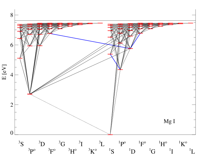
Figure 1: The atomic model for the first ionisation stage of magnesium. The observed J-band line transitions are highlighted in blue.

2.3 Atomic data and spectrum synthesis of J-band magnesium lines

Table 1: Mg i J-band lines

Elem.	$\lambda$	$E_{\rm low}$	lower	$E_{\rm up}$	upper	$log~{}gf$	$log~{}C_{6}$
	Å	[eV]	conf.	[eV]	conf.
(1)	(2)	(3)	(4)	(5)	(6)	(7)	(8)
	11828.185	4.346096	3p 1P${}_{1}^{\mathrm{o}}$	5.394090	4s 1S0	$-$0.305	$-$29.7
	12083.278	5.753635	3d 1D2	6.779505	4f 3F${}_{3}^{\mathrm{o}}$	$-$1.500	$-$29.3
	12083.346	5.753635	3d 1D2	6.779498	4f 3F${}_{2}^{\mathrm{o}}$	$-$1.500	$-$29.3
	12083.662	5.753635	3d 1D2	6.779472	4f 1F${}_{3}^{\mathrm{o}}$	0.050	$-$29.3

The basic information about the observed magnesium lines in the J-band is given in Table 1. The four lines belong to multiplets 175, 224, and 225 (multiplet numbers taken from the NIST online database). The line at 11828.185 Å forms in the transition between the $3p\,^{1}{\rm P}^{{\rm\circ}}$ and $4s\,^{1}{\rm S}$ levels. The three lines around 12083 Å originate in the transitions between $3d\,^{1}{\rm D}$ - $4f\,^{1}{\rm F}^{{\rm\circ}}$, and $3d\,^{1}{\rm D}$ - $4f\,^{3}{\rm F}^{{\rm\circ}}$ levels. In a typical observed spectrum of a late-type star, the three lines from multiplets $224$ and $225$ merge and are thus unresolved. Hereafter, we refer to them as a single line at 12083 Å. However, in the line formation and spectrum synthesis calculations they are treated correctly as three individual lines (see Fig. 6).

Table 2: Stellar parameters of the reference and Per OB1 stars

Star	$T_{\rm eff}$	$\Delta T_{\rm eff}$	$\log g$	$\Delta\log g$	[Z]	$\Delta$ [Z]	$\xi_{t}$
	K		dex		dex		km$/$s
(1)	(2)	(3)	(4)	(5)	(6)	(7)	(8)
Sun	5777	1	4.44	0.00	0.00	0.05	1.00
Arcturus	4286	35	1.64	0.06	$-$0.52	0.08	1.50
BD +56 595	4060	25	0.20	0.70	$-$0.15	0.13	4.00
BD +56 724	3840	25	$-$0.40	0.50	0.08	0.09	3.00
BD +59 372	3920	25	0.50	0.30	$-$0.07	0.09	3.20
HD 13136	4030	25	0.20	0.40	$-$0.10	0.08	4.10
HD 14270	3900	25	0.30	0.30	$-$0.04	0.09	3.70
HD 14404	4010	25	0.20	0.40	$-$0.07	0.10	3.90
HD 14469	3820	25	$-$0.10	0.40	$-$0.03	0.12	4.00
HD 14488	3690	50	0.00	0.20	0.12	0.10	2.90
HD 14826	3930	26	0.10	0.20	$-$0.08	0.07	3.70
HD 236979	4080	25	$-$0.60	0.30	$-$0.09	0.09	3.10

Other than for the optical spectral range where we use oscillator strengths from Chang & Tang (1990) and Aldenius et al. (2007), there are no good experimental $\log gf$ values for the IR Mg I lines. For the $11828.185$ Å  Mg i line, Civis et al (2013) calculated $\log gf=-0.292$, while Tachiev & Froese Fischer (2003) provide $\log gf=-0.333$. We adopt the mean of the two values from the two references, i.e $\log gf=-0.305$.

For the triplet at $12083$ Å, the available data are contradictory. In the Kurucz online database, we find $-2.155$, $-9.300$, $0.553$ for the three lines $12083.278$, $12083.346$, $12083.662$, respectively. For the transition at 12083.662 Å, theoretical calculations by Chang & Tang (1990) and Civis et al. (2013) provide $\log gf=0.41$ and $\log gf=0.44$, respectively. Our previous RSG synthetic grid (see Paper I) included the following values $0.45$, $-0.79$, $0.415$ for the $12083.264$, $12083.346$, $12083.662$, respectively. These datasets come from the VALD database (Kupka et al., 2000), however, as our test calculations have shown, they hugely over-estimate the line depths in the spectrum of the Sun. The values appear to be wrong, e.g. the $\log gf$ value for the semi-forbidden line at 12083.278 Å is as large as the value of the allowed counterpart at 12083.662 Å. In addition, there is a large differences between the Kurucz’ quantum-mechanical values listed in different online tables for the 12083.278 and 12083.346 lines. Given these largely conflicting $gf$-values we decided to extend our NLTE calculations to the Sun with the well established magnesium abundance of $\log(Mg/H)+12=7.53$ (Asplund et al. 2009). We then iterate the $\log gf$ values until we obtain a satisfactory fit of the 12083 Å Mg triplet line complex. We obtain as best fitting values $-1.5$ for the bluer weak components and $0.05$ for the strong red component, respectively. We then carry out Mg NLTE calculations for the red giant star Arcturus using the stellar parameters from Bergemann et al. (2012) as given in Table 2. The observed spectra for the Sun and Arcturus were taken from Kurucz et al. (1984) and Hinkle et al. (1995), respectively. For Arcturus, we adopt a slight $\alpha$-enhancement, [Mg/Fe]$=0.2$, which is also confirmed by the earlier work on abundances by Ramirez & Allende Prieto (2011). The comparison with observed J-band Mg lines for the Sun and Arcturus is shown in Fig. 2 and indicates reasonable agreement.

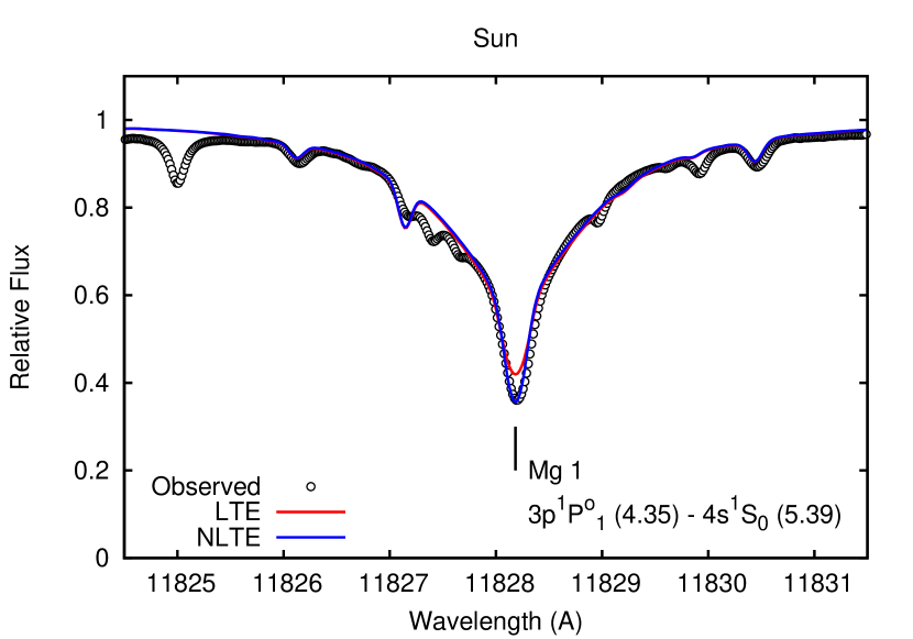
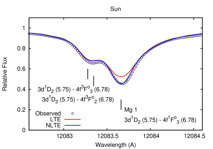
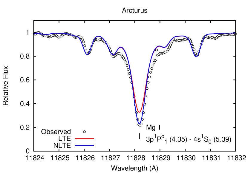
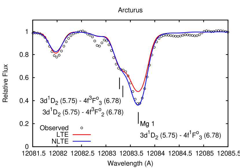
Figure 2: NLTE and LTE line profiles of the Mg i 11828 Å (left) and 12083 Å (right) computed for the Sun (top panels) and Arcturus (bottom panels).

Calculating the relatively strong J-band magnesium lines as in Fig. 2 also requires the inclusion of spectral line broadening. We account for broadening caused by various mechanisms: microturbulence (see Table 2), macro-turbulence, and broadening due to elastic collisions with H i atoms. We tested the $\alpha$ and $\sigma$ coefficients from the Barklem et al. (2000) database of quantum-mechanically calculated values, however these data produce spectral lines which are too weak compared with the observed spectra of our reference stars (Sun, Arcturus). We thus scale these values by $+0.3$ dex. The adopted atomic data are given in Table 1. For macroturbulence we assume the radial-tangential profile, and fit this parameter independently of instrumental profile and rotation. For the red supergiants, we fit a total FWHM which consists of instrumental FWHM and macroturbulence, as the broadening effects cannot be separated in the spectra. The values of the FWHM were taken from Gazak et al. (2014b).

3 NLTE effects in J-band Mg lines

In general, the NLTE effects which we encounter for our grid of RSG atmospheres are very similar to those found by previous studies of cool FGK stars (see Zhao et al. 1998, Shimanskaya et al. 2000, Merle et al. 2011 and references therein). The driving mechanism is normal photospheric photoionisation of neutral magnesium governed by the super-thermal radiation field which escapes the deep photospheres essentially unchanged once its optical depth has dropped below unity. This mechanism works independently of the model atom, of course as long as photoionisation cross-sections are not set to zero. We thus shall not repeat the complete analysis as done in Zhao et al (1998), but only summarise the most important aspects relevant for the atmospheres of RSGs. For the discussion of NLTE effects, it is convenient to employ the concept of energy level departure coefficients, which are defined as

$$b_{i}=n_{i}^{\rm NLTE}/n_{i}^{\rm LTE}$$ (1)

where $n_{i}^{\rm NLTE}$ and $n_{i}^{\rm LTE}$ are NLTE and LTE atomic level populations [cm^-3], respectively.

Fig. 3 shows the departure coefficients $b_{i}$ for a selection of models from our RSG model grid. The diagrams are somewhat different from the conventional 1D representation of $b_{i}$ as a function of optical depth $\tau$ in that on the y-axis we show the level energy, and the colour code indicates the departure coefficient. In this way we obtain a nice overview of the general trend of the NLTE effects as a function of excitation energy. Fig. 4 also shows the conventional representation of the departure coefficients of the upper and lower levels of the J-band transition for the same models as Fig. 3.

The effects of NLTE are clearly seen in this diagram, in particular for energy levels at 4 - 5 eV ($3p\,^{1}{\rm P}^{{\rm\circ}}$, $4s\,^{3}{\rm S}$, $4s\,^{1}{\rm S}$) with large photo-ionisation cross-sections. Ionization by the super-thermal UV radiation field becomes important with proximity to the outer atmospheric boundary, and number densities of energy levels are much lower than the LTE predicts. Conceptually, the behaviour of Mg i atomic number densities bears a strong resemblance with that of Fe i as discussed in detail in Bergemann et al. (2012) and in Paper I.

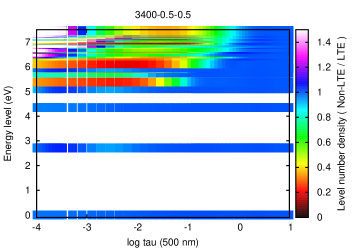
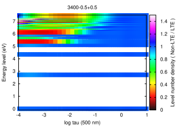
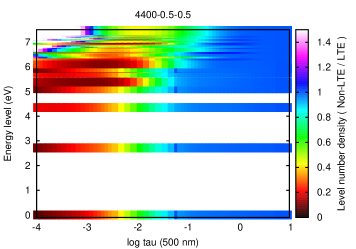
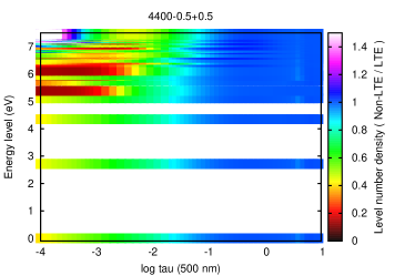
Figure 3: Mg i NLTE departure coefficients in RSG atmospheres shown for a few examples of the model grid. Top: T${}_{\rm eff}=3400$K, log g $=-0.5$ and [Z] $=-0.5$ (left) and $0.5$ (right). Bottom: same as top but T${}_{\rm eff}=4400$K. The value of the departure coefficients is color coded. The y-axis is the excitation energy of the levels and the x-axis is continuum optical depth at 500 nm.

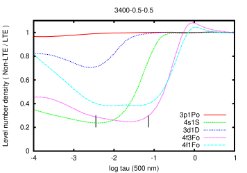
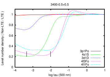
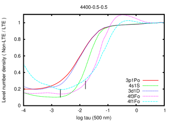
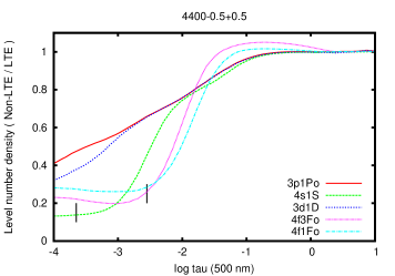
Figure 4: Mg i NLTE departure coefficients of the lower and upper levels of the J-band transitions shown for the same models as in Fig. 3. The NLTE line core optical depths $\log\tau(11828.185$ Å$)=0$ and $\log\tau(12083.662$ Å$)=0$ are also indicated by black vertical marks. The 12083.662 line forms deeper in the atmosphere.

For the IR J-band transitions, the main additional NLTE effect is through radiation transport in the spectral lines themselves. The lower level of the 12083.660 Å line is $3d\,^{1}{\rm D}$ at 5.75 eV, and its only connection to the lower-lying levels, $\,{}^{1}{\rm P}^{{\rm\circ}}$ (4.36 eV) and $\,{}^{3}{\rm P}^{{\rm\circ}}$ (2.71 eV), is via the forbidden magnetic-dipole transitions at $\sim 4070-4080$ Å  ($\,{}^{3}{\rm P}^{{\rm\circ}}$ - $\,{}^{1}{\rm D}$) and the allowed transition in the near-IR (at $8806$ Å, $\,{}^{1}{\rm P}^{{\rm\circ}}_{\rm 1}$ - $\,{}^{1}{\rm D}_{\rm 2}$) respectively (see the energy level diagram, Fig. 1). The lower level of the line at 11823 Å is $3p\,^{1}{\rm P}^{{\rm\circ}}$. The level is connected with the ground state through a resonance line at 2852 Å ($\,{}^{1}{\rm S}$ - $\,{}^{1}{\rm P}^{{\rm\circ}}$), which is optically thick throughout the formation depths of the J-band Mg i lines and does not effectively participate in the NLTE radiation transport. This configuration explains the fact that the both J-band lines have a nearly two-level-atom line source function S_ij. Once the lines have become optically thin, downward cascading electrons over-populate the lower levels of the transitions relative to the upper levels, and the source functions become sub-thermal, S${}_{ij}<$ B_ν (see Fig. 4). Therefore the J-band Mg i lines are stronger in NLTE than in LTE, and the NLTE effect further increases with decreasing $T_{\rm eff}$ and $\log g$. This is a very similar situation to the formation of the J-band silicon lines discussed in Paper II. The resulting differences between the J-band spectral lines profiles in the LTE and non-LTE case are illustrated in Fig. 5.

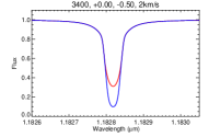
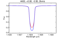
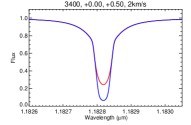
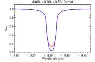
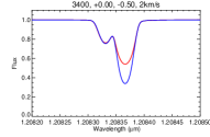
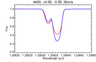
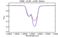
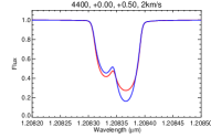
Figure 5: Profiles of the J-band Mg i lines computed in LTE (red) and NLTE (blue) for a few examples of the model atmosphere grid. All models are for $\log g=0.0$ and $\xi_{\rm t}=2$ km$/$s. The upper row is for the line at 11828 Å and the bottom row for 12083 Å.

Beyond this more general discussion of the J-band NLTE effects the formation of the line profiles of the 12083 Å super-line are affected by an additional complication. Since the observed feature is a blend of three Mg I components from different multiplets, the result is a highly asymmetric shape, which varies with stellar parameters (see Fig. 5, bottom four panels). Each of the components suffers from its own NLTE effect. To illustrate this peculiar effect, we provide the profiles of each component computed in LTE and NLTE for the model with $T_{\rm eff}=4400$, $\log g=0.0$, and $[\rm{Fe}/\rm{H}]=0.5$ in Fig. 6. The bluest line at 12083.278 Å  which forms in the 3d ¹D₂ - ³F${}_{3}^{\mathrm{o}}$ transition, is weaker in NLTE than in LTE. With its very small oscillator strength this line forms in the deeper atmospheric layers where the departure coefficient of the upper level is larger than the one of the lower level. The upper levels of the 12083 transitions are very close to the Mg ii continuum at 7.64 eV and are sensitive to recombination cascades from Mg ii, which causes their overpopulation in deeper atmospheric layers. As a consequence, the NLTE source function is super-thermal, S${}_{ij}>$ B_ν. The reddest component at 12083.662 Å has a much larger oscillator strength and forms much further out in the atmosphere, where the departure coefficient of the upper level is always smaller than the one of lower level as already described above.

Figure 6: Individual line components (dashed) contribution to the total profile (solid) of the J-band Mg i line at 12083 Å computed with $T_{\rm eff}=4400$, $\log g=0.0$, and $[\rm{Fe}/\rm{H}]=0.5$ in LTE (top) and NLTE (bottom).

4 NLTE Mg i abundance corrections

Over the whole RSG grid the J-band Mg i absorption lines are stronger in NLTE than in LTE. Quantitatively, this information is summarised in Table 3 which compiles the equivalent widths for two values of microturbulence, 2 and 5 km$/$s. As a consequence, magnesium abundances obtained from a LTE fit of observed J-band lines are systematically too high. This can be quantitatively assessed by introducing NLTE abundance corrections $\Delta$.

$$\Delta_{\rm Mg~{}I}=\log\rm{A(Mg)}_{\rm NLTE}-\log\rm{A(Mg)}_{\rm LTE}$$ (2)

$\Delta_{\rm Mg~{}I}$ is the logarithmic correction, which has to be applied to an LTE magnesium abundance determination of a specific line, $\log\rm{A(Mg)}_{\rm LTE}$, to obtain the correct value corresponding to the use of NLTE line formation. These corrections are obtained at each point of our model grid by matching the NLTE equivalent width through varying the Mg abundance in the LTE calculations. When for the same element abundance the NLTE line equivalent width is larger than the LTE one, it requires a higher LTE abundance to fit the NLTE equivalent width and, thus, the NLTE abundance corrections become negative. Fig. 7 shows the NLTE abundance corrections computed with two values of microturbulence, 2 and 5 km s^-1. The exact values of the NLTE abundance corrections are given in Table 4. The results for Mg are very similar to those we obtained for the J-band Si lines (Paper II). Fig. 8 also shows the effect of varying Mg abundance ([Z] fixed to the solar value) on the line profiles for the both Mg I J-band lines and Fig. 9 illustrates the impact of microturbulence $\xi_{\rm t}$. Clearly, the larger $\xi_{\rm t}$ the stronger a spectral line, demonstrating the fundamental degeneracy between small scale turbulent broadening and abundance. The 11828 Å line and the strongest component of the 12083 Å line usually occupy the flat part of the curve-of-growth and are very sensitive to the microturbulence velocity. In contrast, the two weaker components of the J-band triplet at 12083 Å are on the linear part of the curve-of-growth even in very cool atmospheres ($T_{\rm eff}=3400$ K).

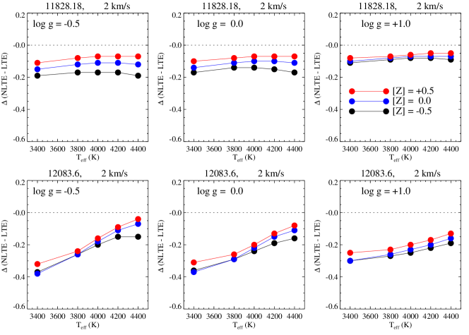
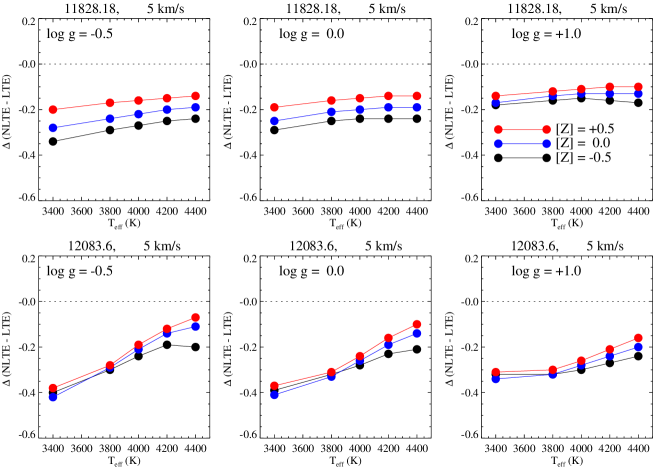
Figure 7: NLTE abundance corrections for the 11828 (top) and 12083 (bottom) Å Mg i lines as a function of effective temperature and metallicity for log g = $-$0.5 (left), 0.0 (middle), and 1.0 (right). Top panels: $\xi_{\rm t}=2$ km s^-1; bottom panels: $\xi_{\rm t}=5$ km s^-1.

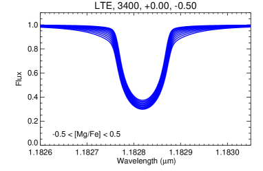
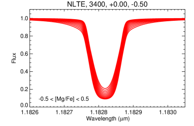
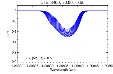
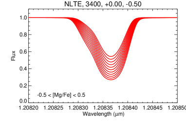
Figure 8: LTE (left) and NLTE (right) lines profiles for the 11828 (top) and 12083 (bottom) Å Mg I lines as a function of Mg abundance. [Mg$/$Fe] varies from $-$0.5 to +0.5 with a step of 0.1 dex.

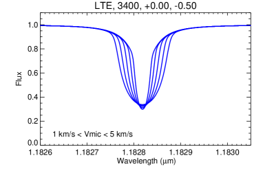
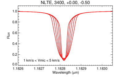
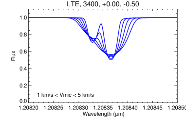
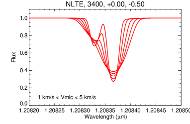
Figure 9: LTE (left) and NLTE (right) lines profiles for the 11828 (top) and 12083 (bottom) Mg i lines as a function of microturbulence. $\xi_{\rm t}$ varies from 1 to 5 km s^-1 with a step of 1 km s^-1.

The NLTE abundance corrections are significant with large negative values between $-0.4$ to $-0.1$ dex and are strongest at low metallicity [Z]. We see a clear trend with effective temperature, the effect being significantly stronger for the 12083 Å line.

5 Mg i J-band lines of Per OB1 red supergiants

Gazak et al. (2014b) investigated high resolution, high S/N J-band spectra of eleven RSGs in the young massive stellar double cluster h and $\chi$ Persei (Per OB1) in the solar neighbourhood as a crucial test of the J-band analysis method. While this test nicely confirmed the reliability of the method with an average cluster metallicity [Z] $=-0.04$ derived from the spectra, the authors excluded the Mg i lines from the analysis (see their Figures 1 and 2) because of the obvious apparent NLTE effects for which no NLTE calculations were available at the time of their analysis work. Now with our new calculations at hand, we can use the stellar parameters determined by Gazak et al. and check whether observed and calculated Mg i J-band line profiles agree.

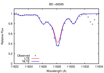
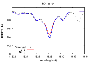
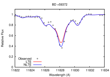
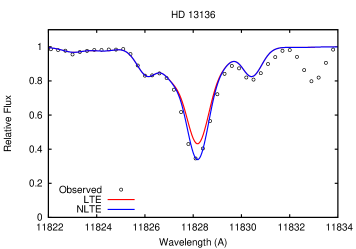
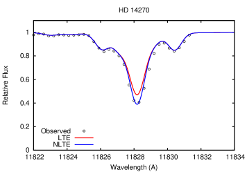
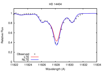
Figure 10: Observed J-band Mg i profiles computed in LTE and NLTE for the atmospheric parameters determined by Gazak et al. (2014b) as given in Table 2.

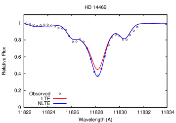
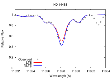
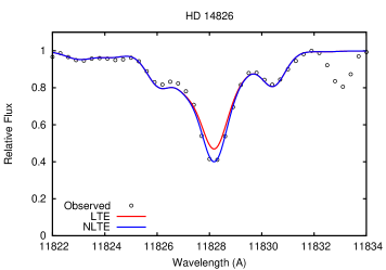
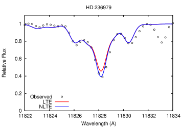
Figure 11: Observed J-band Mg i profiles computed in LTE and NLTE for the atmospheric parameters determined by Gazak et al. (2014b) as given in Table 2.

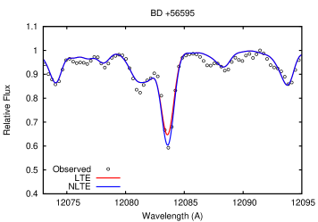
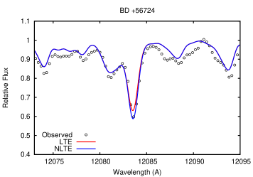
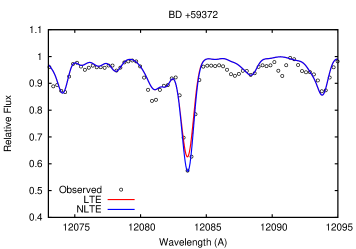
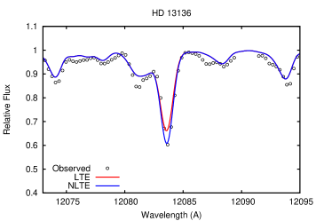
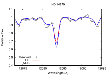
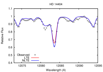
Figure 12: Observed J-band Mg i profiles computed in LTE and NLTE for the atmospheric parameters determined by Gazak et al. (2014b) as given in Table 2.

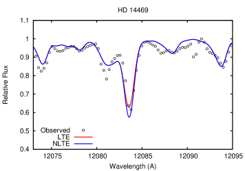
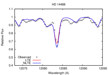
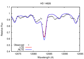
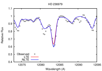
Figure 13: Observed J-band Mg i profiles computed in LTE and NLTE for the atmospheric parameters determined by Gazak et al. (2014b) as given in Table 2.

The comparison of NLTE and LTE fits to Mg I lines for the Per OB-1 spectra of 10 stars is shown in Fig. 10, 11, 12, 13. The stellar parameters are given in Table 2. A solar value is adopted for the [Mg$/$Fe] ratio in the calculation. The agreement between the new NLTE calculations and the observations is much better than with the previous atomic data and LTE. This confirms that for future work the Mg i J-band lines can be used as an additional constraint of metallicity. In addition, since the Mg i lines have the highest excitation potential of the lower levels of their transitions compared to the iron, titanium and silicon lines used so far in the J-band technique, they will also be very useful to constrain effective temperature and gravity. This will strengthen the accuracy of the method significantly.

6 Conclusions

With the new Mg I NLTE calculations presented in this work we are now able to use the full J-band spectrum of atomic lines (iron, titanium, silicon and magnesium) for a detailed analysis of red supergiant stars. This is an important step forward for the IR spectroscopy of bright stars in the Milky Way, e.g. individual RSGs (see for instance Gazak et al. 2014b), but also extra-galactic stellar populations, such as young and very massive super star clusters for which the J-band spectra are completely dominated by RSGs once they are older than 7 Myr. Gazak et al. (2014a) have demonstrated that the J-band technique applied to SSCs yields reliable metallicities, but the accuracy of them was somewhat compromised by the fact that the Mg i lines could not be used because of the importance of NLTE effects. With the new calculations available it will be possible to significantly improve this work and to fully use the tremendous potential of the J-band method.

Table 3: Equivalent widths of the Mg i lines ($\xi_{t}$ = 2 and 5 kms^-1)

Teff	$log~{}g$	[Z]			$\xi_{t}$ = 2 kms-1			$\xi_{t}$ = 5 kms-1
			$W_{\lambda,\rm MgI}$	$W_{\lambda,\rm MgI}$	$W_{\lambda,\rm MgI}$	$W_{\lambda,\rm MgI}$	$W_{\lambda,\rm MgI}$	$W_{\lambda,\rm MgI}$	$W_{\lambda,\rm MgI}$	$W_{\lambda,\rm MgI}$
			$11828$	$11828$	$12083$	$12083$	$11828$	$11828$	$12083$	$12083$
			$LTE$	$NLTE$	$LTE$	$NLTE$	$LTE$	$NLTE$	$LTE$	$NLTE$
(1)	(2)	(3)	(4)	(5)	(6)	(7)	(8)	(9)	(10)	(11)
4400	$-$0.50	0.00	483.2	511.7	404.8	413.5	847.2	899.6	575.2	597.0
4400	$-$0.50	0.50	582.9	608.4	501.5	504.1	972.6	1021.3	719.8	730.0
4400	$-$0.50	$-$0.50	403.5	436.8	300.6	323.4	721.9	782.3	426.3	468.0
4200	$-$0.50	0.00	519.9	553.1	425.5	439.8	888.8	951.9	607.3	636.0
4200	$-$0.50	0.50	640.5	671.9	519.9	531.6	1021.6	1083.8	748.3	771.3
4200	$-$0.50	$-$0.50	434.1	469.7	326.3	348.9	770.5	836.6	464.4	505.0
4000	$-$0.50	0.00	554.9	597.3	427.8	452.7	911.0	991.9	612.0	655.5
4000	$-$0.50	0.50	696.7	738.0	516.4	539.9	1052.4	1133.3	744.8	784.7
4000	$-$0.50	$-$0.50	459.7	502.4	336.8	366.4	795.8	875.9	480.3	530.4
3800	$-$0.50	0.00	577.7	632.6	408.4	444.8	906.4	1009.8	585.0	644.9
3800	$-$0.50	0.50	730.5	784.7	491.3	526.8	1053.2	1155.8	708.8	766.7
3800	$-$0.50	$-$0.50	475.7	528.9	326.4	365.0	795.1	894.3	465.8	528.0
3400	$-$0.50	0.00	554.6	629.2	314.4	366.7	830.0	967.5	449.8	531.3
3400	$-$0.50	0.50	709.0	780.3	394.5	443.6	989.5	1120.5	566.4	644.8
3400	$-$0.50	$-$0.50	456.6	530.2	246.9	297.1	719.7	855.6	352.4	426.7
4400	0.00	0.00	497.3	529.2	400.3	414.6	840.7	900.1	567.0	596.2
4400	0.00	0.50	612.5	641.8	500.6	509.9	980.1	1036.4	715.5	735.4
4400	0.00	$-$0.50	410.1	445.9	299.2	323.6	712.9	778.4	423.1	466.1
4400	1.00	0.00	592.0	626.4	394.8	419.7	872.8	938.2	549.1	591.0
4400	1.00	0.50	755.4	791.0	497.4	519.7	1049.4	1117.0	694.9	731.8
4400	1.00	$-$0.50	466.3	501.8	296.2	326.5	718.8	784.6	412.6	460.9
4200	0.00	0.00	540.7	577.9	414.1	435.8	881.4	951.6	588.4	627.4
4200	0.00	0.50	677.6	713.5	510.0	529.3	1027.6	1098.0	730.2	764.3
4200	0.00	$-$0.50	443.1	482.4	317.7	345.6	754.6	827.8	450.5	497.9
4200	1.00	0.00	662.6	704.0	396.7	429.6	924.2	1002.1	550.3	603.1
4200	1.00	0.50	845.1	890.1	493.1	524.5	1108.5	1192.4	685.6	735.3
4200	1.00	$-$0.50	523.4	562.6	305.2	340.6	768.6	841.9	424.2	479.4
4000	0.00	0.00	581.9	628.6	409.4	441.3	902.3	990.8	581.9	635.5
4000	0.00	0.50	732.6	779.6	497.7	528.5	1052.2	1141.9	712.5	763.1
4000	0.00	$-$0.50	475.1	521.1	321.8	356.9	779.5	865.5	456.7	513.7
4000	1.00	0.00	725.1	777.2	381.6	422.3	958.3	1053.6	526.8	590.0
4000	1.00	0.50	919.1	975.4	471.9	512.5	1150.6	1253.8	650.8	713.3
4000	1.00	$-$0.50	577.4	623.7	298.1	339.4	803.2	887.6	412.5	475.1
3800	0.00	0.00	611.7	671.0	385.2	427.1	900.2	1010.7	546.9	614.7
3800	0.00	0.50	773.3	832.6	467.5	509.2	1057.8	1168.5	667.9	734.3
3800	0.00	$-$0.50	498.7	554.6	306.7	348.8	781.9	885.3	434.9	500.9
3800	1.00	0.00	749.8	813.4	348.5	395.3	957.4	1071.5	478.3	548.8
3800	1.00	0.50	940.6	1007.5	434.3	481.7	1152.5	1273.3	593.7	665.6
3800	1.00	$-$0.50	608.6	664.2	273.5	318.2	810.5	908.7	376.3	441.3
3400	0.00	0.00	570.6	645.1	287.0	339.0	816.8	953.0	406.3	485.8
3400	0.00	0.50	719.3	791.3	365.4	414.9	977.0	1108.6	518.5	596.1
3400	0.00	$-$0.50	472.0	544.3	222.4	271.0	703.6	834.4	314.1	384.2
3400	1.00	0.00	642.1	708.7	245.1	292.6	836.8	953.3	334.1	402.2
3400	1.00	0.50	795.3	864.0	322.2	368.1	1008.0	1129.9	439.0	507.7
3400	1.00	$-$0.50	536.7	596.8	186.0	228.7	713.4	815.2	252.1	310.2

Table 4: Non-LTE abundance corrections for the Mg i lines ($\xi_{t}$ = 2 and 5 kms^-1)

Teff	$log~{}g$	[Z]	$\xi_{t}$ = 2 kms-1		$\xi_{t}$ = 5 kms-1
			$\Delta_{\rm MgI}$	$\Delta_{\rm MgI}$	$\Delta_{\rm MgI}$	$\Delta_{\rm MgI}$
			$11828$	$12083$	$11828$	$12083$
(1)	(2)	(3)	(4)	(5)	(6)	(7)
4400.	1.00	0.50	$-$0.05	$-$0.10	$-$0.11	$-$0.13
4400.	1.00	0.00	$-$0.07	$-$0.12	$-$0.14	$-$0.16
4400.	1.00	$-$0.50	$-$0.10	$-$0.16	$-$0.18	$-$0.19
4400.	0.00	0.50	$-$0.07	$-$0.05	$-$0.15	$-$0.07
4400.	0.00	0.00	$-$0.12	$-$0.08	$-$0.20	$-$0.11
4400.	0.00	$-$0.50	$-$0.18	$-$0.13	$-$0.25	$-$0.17
4400.	$-$0.50	0.50	$-$0.08	$-$0.01	$-$0.15	$-$0.04
4400.	$-$0.50	0.00	$-$0.13	$-$0.05	$-$0.20	$-$0.08
4400.	$-$0.50	$-$0.50	$-$0.20	$-$0.12	$-$0.25	$-$0.16
4200.	1.00	0.50	$-$0.06	$-$0.14	$-$0.11	$-$0.17
4200.	1.00	0.00	$-$0.07	$-$0.16	$-$0.14	$-$0.19
4200.	1.00	$-$0.50	$-$0.09	$-$0.18	$-$0.17	$-$0.22
4200.	0.00	0.50	$-$0.07	$-$0.10	$-$0.15	$-$0.13
4200.	0.00	0.00	$-$0.11	$-$0.12	$-$0.20	$-$0.15
4200.	0.00	$-$0.50	$-$0.16	$-$0.15	$-$0.25	$-$0.19
4200.	$-$0.50	$-$0.50	$-$0.18	$-$0.12	$-$0.26	$-$0.15
4200.	$-$0.50	0.50	$-$0.07	$-$0.07	$-$0.16	$-$0.09
4200.	$-$0.50	0.00	$-$0.12	$-$0.08	$-$0.21	$-$0.11
4000.	1.00	0.50	$-$0.06	$-$0.17	$-$0.12	$-$0.21
4000.	1.00	0.00	$-$0.08	$-$0.19	$-$0.15	$-$0.23
4000.	1.00	$-$0.50	$-$0.09	$-$0.21	$-$0.17	$-$0.24
4000.	0.00	0.50	$-$0.08	$-$0.16	$-$0.16	$-$0.19
4000.	0.00	0.00	$-$0.11	$-$0.18	$-$0.21	$-$0.21
4000.	0.00	$-$0.50	$-$0.15	$-$0.19	$-$0.26	$-$0.23
4000.	$-$0.50	0.50	$-$0.08	$-$0.13	$-$0.17	$-$0.16
4000.	$-$0.50	0.00	$-$0.12	$-$0.14	$-$0.23	$-$0.17
4000.	$-$0.50	$-$0.50	$-$0.18	$-$0.16	$-$0.28	$-$0.19
3800.	1.00	0.50	$-$0.07	$-$0.19	$-$0.13	$-$0.24
3800.	1.00	0.00	$-$0.09	$-$0.22	$-$0.16	$-$0.26
3800.	1.00	$-$0.50	$-$0.10	$-$0.23	$-$0.17	$-$0.26
3800.	0.00	0.50	$-$0.08	$-$0.22	$-$0.17	$-$0.26
3800.	0.00	0.00	$-$0.12	$-$0.24	$-$0.23	$-$0.27
3800.	0.00	$-$0.50	$-$0.15	$-$0.24	$-$0.27	$-$0.27
3800.	$-$0.50	0.50	$-$0.09	$-$0.20	$-$0.18	$-$0.23
3800.	$-$0.50	0.00	$-$0.13	$-$0.21	$-$0.25	$-$0.24
3800.	$-$0.50	$-$0.50	$-$0.18	$-$0.22	$-$0.31	$-$0.25
3400.	1.00	0.50	$-$0.09	$-$0.21	$-$0.15	$-$0.26
3400.	1.00	0.00	$-$0.11	$-$0.25	$-$0.18	$-$0.28
3400.	1.00	$-$0.50	$-$0.12	$-$0.26	$-$0.19	$-$0.27
3400.	0.00	0.50	$-$0.11	$-$0.27	$-$0.20	$-$0.31
3400.	0.00	0.00	$-$0.15	$-$0.31	$-$0.26	$-$0.35
3400.	0.00	$-$0.50	$-$0.18	$-$0.31	$-$0.31	$-$0.32
3400.	$-$0.50	0.50	$-$0.11	$-$0.28	$-$0.21	$-$0.32
3400.	$-$0.50	0.00	$-$0.16	$-$0.32	$-$0.30	$-$0.36
3400.	$-$0.50	$-$0.50	$-$0.21	$-$0.32	$-$0.36	$-$0.33

References

- Allen (1973) Allen, C. W. 1973, London: University of London, Athlone Press, —c1973, 3rd ed.,
- Allende Prieto et al. (2001) Allende Prieto, C., Lambert, D. L., & Asplund, M. 2001, ApJ, 556, L63
- Asplund et al. (2009) Asplund, M., Grevesse, N., Sauval, A. J., & Scott, P. 2009, ARA&A, 47, 481
- Barklem et al. (2000) Barklem, P. S., Piskunov, N., & O’Mara, B. J. 2000, VizieR Online Data Catalog, 414, 20467
- Barklem et al. (2011) Barklem, P. S., Belyaev, A. K., Guitou, M., et al. 2011, A&A, 530, A94
- Barklem et al. (2012) Barklem, P. S., Belyaev, A. K., Spielfiedel, A., Guitou, M., & Feautrier, N. 2012, A&A, 541, AA80
- Bergemann et al. (2012) Bergemann, M., Kudritzki, R.- P., Plez, B., et al. 2012, ApJ, 751, 156
- Bergemann et al. (2012) Bergemann, M., Hansen, C. J., Bautista, M., & Ruchti, G. 2012, A&A, 546, A90
- Bergemann et al. (2012) Bergemann, M., Lind, K., Collet, R., Magic, Z., & Asplund, M. 2012, MNRAS, 427, 27
- Bresolin et al. (2009) Bresolin, F., Gieren, W., Kudritzki, R.-P., et al. 2009, ApJ, 700, 309
- Bresolin et al. (2011) Bresolin, F., 2011, ApJ 729, 56
- Bresolin et al. (2012) Bresolin, F., Kennicutt, R.C., Ryan-Weber, E., 2012, ApJ 750, 122
- Brooke et al. (2014) Brooke, J. S. A., Ram, R. S., Western, C. M., et al. 2014, ApJS, 210, 23
- Brott & Hauschildt (2005) Brott, A. M., Hauschildt, P. H., “A PHOENIX Model Atsmophere Grid for GAIA”, ESAsp, 567, 565
- Butler & Giddings (1985) Butler, K., Giddings, J. 1985, Newsletter on Analysis of Astronomical Spectra No. 9, University College London
- Chiavassa et al. (2011) Chiavassa, A., Freytag, B., Masseron, T., & Plez, B. 2011, A&A, 535, A22
- Cox (2000) Cox, A. N. 2000, Allen’s Astrophysical Quantities
- Cunto et al. (1993) Cunto W., Mendoza C., Ochsenbein F., Zeippen C.J., 1993, A&A 275, L5
- Davies et al. (2010) Davies, B., Kudritzki, R. P., & Figer, D. F. 2010, MNRAS, 407, 1203
- Davies et al. (2013) Davies, B., Kudritzki, R.P., Plez, B., et al., 2013, ApJ 767, 3
- Davies et al. (2014) Davies, B., Kudritzki, R.P., Gazak, J.Z., Plez, B., Bergemann, M., Evans, C.J., Patrick, L.R., 2014, submitted to ApJ
- Evans et al. (2011) Evans, C. J., Davies, B., Kudritzki, R. P., et al. 2011, A&A, 527, 50
- Gazak et al. (2014a) Gazak, J. Z., Davies, B., Bastian, N., et al. 2014, ApJ, 787, 142, (a)
- Gazak et al. (2014b) Gazak, J. Z., Davies, B., Kudritzki, R., Bergemann, M., & Plez, B. 2014, ApJ, 788, 58, (b)
- Gazak et al. (2014c) Gazak, J. Z., 2014, ”Red Supergiants as Luminous Beracons of Cosmic Chemical Abundance: The Infrared J-band Spectroscopic Technique”, Thesis, Institute for Astronomy, University of Hawaii at Manoa, (c)
- Grevesse et al. (2007) Grevesse, N., Asplund, M,& Sauval, A. J. 2007, Space Sci. Rev., 130, 105
- Gustafsson et al. (2008) Gustafsson, B., Edvardsson, B., Eriksson, K., Jorgensen, U. G., Nordlund, A, & Plez, B. 2008, A&A, 486, 951
- Hinkle et al. (1995) Hinkle, K., Wallace, L., & Livingston, W. 1995, PASP, 107, 1042
- Humphreys & Davidson (1979) Humphreys, R. M., & Davidson, K. 1979, ApJ, 232, 409
- Kramida et al. (2012) Kramida, A., Ralchenko, Yu., Reader, J., and NIST ASD Team (2012). NIST Atomic Spectra Database (ver. 5.0), [Online]. Available: http://physics.nist.gov/asd [2012, August 6]. National Institute of Standards and Technology, Gaithersburg, MD
- Kudritzki et al. (2008) Kudritzki, R.-P., Urbaneja, M. A., Bresolin, F., et al. 2008, ApJ, 681, 269
- Kudritzki et al. (2012) Kudritzki, R.-P., Urbaneja, M. A., Gazak, Z., et al. 2012, ApJ, 747, 15
- Kudritzki et al. (2013) Kudritzki, R.P., Urbaneja, M.A., Gazak, J.Z., Macri, L., Hosek, M.W., Bresolin, F., Przybilla, N., 2013, ApJ 779, L20
- Kudritzki et al. (2014) Kudritzki, R.P., Urbaneja, M.A., Bresolin, F., Hosek, M.W., Przybilla, N., 2014, ApJ 788, 56
- Kurucz et al. (1984) Kurucz, R. L., Furenlid, I., Brault, J., & Testerman, L. 1984, National Solar Observatory Atlas, Sunspot, New Mexico: National Solar Observatory, 1984
- Kurucz (2007) Kurucz, R.-L. 2007, ”Robert L. Kurucz on-line database of observed and predicted atomic transitions”, kurucz.harvard.edu
- Kupka et al. (2000) Kupka, F. G., Ryabchikova, T. A., Piskunov, N. E., Stempels, H. C., & Weiss, W. W. 2000, Baltic Astronomy, 9, 590
- Lambert (1993) Lambert, D. L. 1993, Physica Scripta Volume T, 47, 186
- Mashonkina (2013) Mashonkina, L. 2013, A&A, 550, AA28
- Merle et al. (2011) Merle, T., Thévenin, F., Pichon, B., & Bigot, L. 2011, MNRAS, 418, 863
- Patrick et al. (2014) Patrick, L.R., Evans, C.J., Davies, B., Kudritzki, R.P., Gazak, J.Z., Bergemann, M., Plez, B., Ferguson, A.M.N., 2014, submitted to ApJ
- Plez (1998) Plez, B. 1998, A&A, 337, 495
- Plez (2010) Plez, B. 2010, ASPC 425, 124
- van Regemorter (1962) van Regemorter, H. 1962, ApJ, 136, 906
- Ramírez & Allende Prieto (2011) Ramírez, I., & Allende Prieto, C. 2011, ApJ, 743, 135
- Reetz (1999) Reetz, J. 1999, PhD thesis, LMU München
- Seaton (1962) Seaton, M. J. 1962, Atomic and Molecular Processes, 375
- Shimanskaya et al. (2000) Shimanskaya, N. N., Mashonkina, L. I., & Sakhibullin, N. A. 2000, Astronomy Reports, 44, 530
- Shi et al. (2008) Shi, J. R., Gehren, T., Butler, K., Mashonkina, L. I., Zhao, G. 2008, A&A, 486, 303
- Steenbock & Holweger (1984) Steenbock, W., & Holweger, H. 1984, A&A, 130, 319
- Wedemeyer (2001) Wedemeyer, S. 2001, A&A, 373, 998
- Zhao et al. (1998) Zhao, G., Butler, K., & Gehren, T. 1998, A&A, 333, 219