Fast Label Embeddings via Randomized Linear Algebra

Abstract

Many modern multiclass and multilabel problems are characterized by increasingly large output spaces. For these problems, label embeddings have been shown to be a useful primitive that can improve computational and statistical efficiency. In this work we utilize a correspondence between rank constrained estimation and low dimensional label embeddings that uncovers a fast label embedding algorithm which works in both the multiclass and multilabel settings. The result is a randomized algorithm whose running time is exponentially faster than naive algorithms. We demonstrate our techniques on two large-scale public datasets, from the Large Scale Hierarchical Text Challenge and the Open Directory Project, where we obtain state of the art results.

1 Introduction

Recent years have witnessed the emergence of many multiclass and multilabel datasets with increasing number of possible labels, such as ImageNet [12] and the Large Scale Hierarchical Text Classification (LSHTC) datasets [25]. One could argue that all problems of vision and language in the wild have extremely large output spaces.

When the number of possible outputs is modest, multiclass and multilabel problems can be dealt with directly (via a max or softmax layer) or with a reduction to binary classification. However, when the output space is large, these strategies are too generic and do not fully exploit some of the common properties that these problems exhibit. For example, often the alternatives in the output space have varying degrees of similarity between them so that typical examples from similar classes tend to be closer to each other than from dissimilar classes. More concretely, classifying an image of a Labrador retriever as a golden retriever is a more benign mistake than classifying it as a rowboat.

Shouldn’t these problems then be studied as structured prediction problems, where an algorithm can take advantage of the structure? That would be the case if for every problem there was an unequivocal structure (e.g. a hierarchy) that everyone agreed on and that structure was designed with the goal of being beneficial to a classifier. When this is not the case, we can instead let the algorithm uncover a structure that matches its own capabilities.

In this paper we use label embeddings as the underlying structure that can help us tackle problems with large output spaces, also known as extreme classification problems. Label embeddings can offer improved computational efficiency because the embedding dimension is much smaller than the dimension of the output space. If designed carefully and applied judiciously, embeddings can also offer statistical efficiency because the number of parameters can be greatly reduced without increasing, or even reducing, generalization error.

1.1 Contributions

We motivate a particular label embedding defined by the low-rank approximation of a particular matrix, based upon a correspondence between label embedding and the optimal rank-constrained least squares estimator. Assuming realizability and infinite data, the matrix being decomposed is the expected outer product of the conditional label probabilities. In particular, this indicates two labels are similar when their conditional probabilities are linearly dependent across the dataset. This unifies prior work utilizing the confusion matrix for multiclass [5] and the empirical label covariance for multilabel [42].

We apply techniques from randomized linear algebra [19] to develop an efficient and scalable algorithm for constructing the embeddings, essentially via a novel randomized algorithm for rank-constrained squared loss regression. Intuitively, this technique implicitly decomposes the prediction matrix of a model which would be prohibitively expensive to form explicitly. The first step of our algorithm resembles compressed sensing approaches to extreme classification that use random matrices [21]. However our subsequent steps tune the embeddings to the data at hand, providing the opportunity for empirical superiority.

2 Algorithm Derivation

2.1 Notation

We denote vectors by lowercase letters $x$, $y$ etc. and matrices by uppercase letters $W$, $Z$ etc. The input dimension is denoted by $d$, the output dimension by $c$ and the embedding dimension by $k$. For multiclass problems $y$ is a one hot (row) vector (i.e. a vertex of the $c-1$ unit simplex) while for multilabel problems $y$ is a binary vector (i.e. a vertex of the unit $c$-cube). For an $m\times n$ matrix $X\in\mathbb{R}^{m\times n}$ we use $||X||_{F}$ for its Frobenius norm, $X^{\dagger}$ for the pseudoinverse, $\Pi_{X,L}$ for the projection onto the left singular subspace of $X$, and $X_{1:k}$ for the matrix resulting by taking the first $k$ columns of $X$. We use $X^{*}$ to denote a matrix obtained by solving an optimization problem over matrix parameter $X$. The expectation of a random variable $v$ is denoted by $\mathbb{E}[v]$.

2.2 Background

Algorithm 1 Randomized PCA

1:

2:function RPCA($k,X\in\mathbb{R}^{n\times d}$)

3:     $(p,q)\leftarrow(20,1)$ $\triangleright$ These hyperparameters rarely need adjustment.

4:     $Q\leftarrow\operatorname{randn}(d,k+p)$

5:     for $i\in\{1,\ldots,q\}$ do $\triangleright$ Randomized range finder for $X^{\top}X$

6:         $\Psi\leftarrow X^{\top}XQ$ $\triangleright$ $\Psi$ can be computed in one pass over the data

7:         $Q\leftarrow\operatorname{orthogonalize}(\Psi)$ $\triangleright$ orth complexity $O(dk^{2})$ is independent of $n$

8:     end for $\triangleright$ NB: total of $(q+1)$ data passes, including next line

9:     $F\leftarrow(X^{\top}XQ)^{\top}(X^{\top}XQ)$ $\triangleright$ $F\in\mathbb{R}^{(k+p)\times(k+p)}$ is “small’

10:     $(V,\Sigma^{2})\leftarrow\operatorname{eig}(F,k)$ $\triangleright$ Exact optimization on small matrix

11:     $V\leftarrow(X^{\top}XQ)V\Sigma^{\dagger}$ $\triangleright$ Back out the solution

12:     return $(V,\Sigma)$

13:end function

In this section we offer an informal discussion of randomized algorithms for approximating the principal components analysis of a data matrix $X\in\mathbb{R}^{n\times d}$ with $n$ examples and $d$ features. For a very thorough and more formal discussion see [19].

Algorithm 1 shows a recipe for performing randomized PCA. In both theory and practice, the algorithm is insensitive to the parameters $p$ and $q$ as long as they are large enough (in our experiments we use $p=20$ and $q=1$). We start with a set of $k+p$ random vectors and use them to probe the range of $X^{\top}X$. Since principal eigenvectors can be thought as “frequent directions” [28], the range of $\Psi$ will tend to be more aligned with the space spanned by the top eigenvectors of $X^{\top}X$. We compute an orthogonal basis for the range of $\Psi$ and repeat the process $q$ times. This can also be thought as orthogonal (aka subspace) iteration for finding eigenvectors with the caveat that we early stop (i.e., $q$ is small). Once we are done and we have a good approximation for the principal subspace of $X^{\top}X$, we optimize fully over that subspace and back out the solution. The last few steps are cheap because we are only working with a $(k+p)\times(k+p)$ matrix and the largest bottleneck is either the computation of $\Psi$ in a single machine setting or the orthogonalization step if parallelization is employed. An important observation we use below is that $X$ or $X^{\top}X$ need not be available explicitly; to run the algorithm we only need to be able to compute the result of multiplying with $X^{\top}X$.

2.3 Rank-Constrained Estimation and Embedding

Algorithm 2 Rembrandt: Response EMBedding via RANDomized Techniques. A reference implementation is publicly available.[32]

1:

2:function Rembrandt($k,X\in\mathbb{R}^{n\times d},Y\in\mathbb{R}^{n\times c}$)

3:     $(p,q)\leftarrow(20,1)$ $\triangleright$ These hyperparameters rarely need adjustment.

4:     $Q\leftarrow\operatorname{randn}(c,k+p)$

5:     for $i\in\{1,\ldots,q\}$ do $\triangleright$ Randomized range finder for $Y^{\top}\Pi_{X,L}Y$

6:         $Z\leftarrow\operatorname*{arg\,min}\|YQ-XZ\|^{2}_{F}$

7:         $Q\leftarrow\operatorname{orthogonalize}(Y^{\top}XZ)$

8:     end for $\triangleright$ NB: total of $(q+1)$ data passes, including next line

9:     $F\leftarrow(Y^{\top}XZ)^{\top}(Y^{\top}XZ)$ $\triangleright$ $F\in\mathbb{R}^{(k+p)\times(k+p)}$ is “small”

10:     $(V,\Sigma^{2})\leftarrow\operatorname{eig}(F,k)$

11:     $V\leftarrow(Y^{\top}XZ)V\Sigma^{\dagger}$ $\triangleright$ $V\in\mathbb{R}^{c\times k}$ is the embedding

12:     return $(V,\Sigma)$

13:end function

We begin with a setting superficially unrelated to label embedding. Suppose we seek an optimal squared loss predictor of a high-cardinality target vector $y\in\mathbb{R}^{c}$ which is linear in a high dimensional feature vector $x\in\mathbb{R}^{d}$. Due to sample complexity concerns, we impose a low-rank constraint on the weight matrix. In matrix form,

$$W^{*} =\operatorname*{arg\,min}_{W\in\mathbb{R}^{d\times c}|\operatorname{rank}(W)\leq k}\|Y-XW\|^{2}_{F},$$ (1)

where $Y\in\mathbb{R}^{n\times c}$ and $X\in\mathbb{R}^{n\times d}$ are the target and design matrices respectively. This is a special case of a more general problem studied by [14]; specializing their result yields the solution $W^{*}=X^{\dagger}(\Pi_{X,L}Y)_{k}$, where $\Pi_{X,L}$ projects onto the left singular subspace of $X$, and $(\cdot)_{k}$ denotes optimal Frobenius norm rank-$k$ approximation, which can be computed via SVD. The expression for $W^{*}$ can be written in terms of the SVD $\Pi_{X,L}Y=U\Sigma V^{\top}$, which, after simple algebra, yields $W^{*}=\left(X^{\dagger}(YV_{1:k})\right)V_{1:k}^{\top}$. This is equivalent to the following procedure:

1. $YV_{1:k}$: Project $Y$ down to $k$ dimensions using the top right singular vectors of $\Pi_{X,L}Y$.

2. $X^{\dagger}(YV_{1:k})$ Least squares fit the projected labels using $X$ and predict them.

3. $\left(X^{\dagger}(YV_{1:k})\right)V_{1:k}^{\top}$: Map predictions to the original output space, using the transpose of the top right singular vectors of $\Pi_{X,L}Y$.

This motivates the use of the right singular vectors of $\Pi_{X,L}Y$ as a label embedding. The $\Pi_{X,L}Y$ term can be demystified: it corresponds to the predictions of the optimal unconstrained model,

$$Z^{*} =\operatorname*{arg\,min}_{Z\in\mathbb{R}^{d\times c}}\|Y-XZ\|^{2}_{F},$$

$$\Pi_{X,L}Y =XZ^{*}\mathrel{\overset{\makebox[0.0pt]{\mbox{\tiny def}}}{=}}\hat{Y}.$$

The right singular vectors $V$ of $\Pi_{X,L}Y$ are therefore the eigenvectors of $\hat{Y}^{\top}\hat{Y}$, i.e., the matrix formed by the sum of outer products of the optimal unconstrained model’s predictions on each example. Note that actually computing and materializing $Z^{*}\in\mathbb{R}^{d\times c}$ would be expensive; a key aspect of the randomized algorithm is that we get the same result while avoiding this intermediate. In particular we can find the product of $\Pi_{X,L}Y$ with another matrix $Q\in\mathbb{R}^{c\times k}$ via

$$Z^{*}Q =\operatorname*{arg\,min}_{Z\in\mathbb{R}^{d\times k}}\|YQ-XZ\|^{2}_{F},$$

$$\Pi_{X,L}YQ =XZ^{*}Q.$$ (2)

Because squared loss is a proper scoring rule it is minimized at the conditional mean. In the limit of infinite training data ($n\to\infty$) and sufficient model flexibility (so that $\hat{y}=\mathbb{E}[y|x]$) we have that

$$\frac{1}{n}\hat{Y}^{\top}\hat{Y}\stackrel{{\scriptstyle\textrm{a.s.}}}{{\longrightarrow}}\mathbb{E}[\mathbb{E}[y|x]^{\top}\mathbb{E}[y|x]]$$ (3)

by the strong law of large numbers. An embedding based upon the eigendecomposition of $\mathbb{E}[\mathbb{E}[y|x]^{\top}\mathbb{E}[y|x]]$ is not practically actionable, but does provide valuable insights. For example, the principal label space transformation of [42] is an eigendecomposition of the empirical label covariance $Y^{\top}Y$. This is a plausible approximation to $\mathbb{E}[\mathbb{E}[y|x]^{\top}\mathbb{E}[y|x]]$ in the multilabel case. However, for multiclass (or multilabel where most examples have at most one nonzero component), the low-rank constraint alone cannot produce good generalization if the input representation is sufficiently flexible; the eigendecomposition of the prediction covariance will merely select a basis for the $k$ most frequent labels due to the absence of empirical cooccurence statistics. Under these conditions we must further regularize (i.e., tradeoff variance for bias) beyond the low-rank constraint, so that $\hat{Y}$ better approximates $\mathbb{E}[Y|X]$ rather than the observed $Y$. Our procedure admits tuning the bias-variance tradeoff via choice of model (features) used in line 6 of Algorithm 2.

2.4 Rembrandt

Our proposal is Rembrandt, described in Algorithm 2. In the previous section, we motivated the use of the top right singular space of $\Pi_{X,L}Y$ as a label embedding, or equivalently, the top principal components of $Y^{\top}\Pi_{X,L}Y$ (leveraging the fact that the projection is idempotent). Using randomized techniques, we can decompose this matrix without explicitly forming it, because we can compute the product of $\Pi_{X,L}Y$ with another matrix $Q$ via equation 2. Algorithm 2 is a specialization of randomized PCA to this particular form of the matrix multiplication operator. Starting from a random label embedding which satisfies the conditions for randomized PCA (e.g., a Gaussian random matrix), the algorithm first fits the embedding, outer products the embedding with the labels, orthogonalizes and repeats for some number of iterations. Then a final exact eigendecomposition is used to remove the additional dimensions of the embedding that were added to improve convergence. Note that the optimization of 2 is over $\mathbb{R}^{d\times(k+p)}$, not $\mathbb{R}^{d\times c}$, although the result is equivalent; this is the main computational advantage of our technique.

The connection to compressed sensing approaches to extreme classification is now clear, as the random sensing matrix corresponds to the starting point of the iterations in Algorithm 2. In other words, compressed sensing corresponds to Algorithm 2 with $q=0$ and $p=0$, which results in a whitened random projection of the labels as the embedding. Additional iterations ($q>0$) and oversampling ($p>0$) improve the approximation of the top eigenspace, hence the potential for improved performance. However when the model is sufficiently flexible, an embedding matrix which ignores the training data might be superior to one which overfits the training data.

Equation (2) is inexpensive to compute. The matrix vector product $YQ$ is a sparse matrix-vector product so complexity $O(nsk)$ depends only on the average (label) sparsity per example $s$ and the embedding dimension $k$, and is independent of the number of classes $c$. The fit is done in the embedding space and therefore is independent of the number of classes $c$, and the outer product with the predicted embedding is again a sparse product with complexity $O(nsk)$. The orthogonalization step is $O(ck^{2})$, but this is amortized over the data set and essentially irrelevant as long as $n>c$. While random projection theory suggests $k$ should grow logarithmically with $c$, this is only a mild dependence on the number of classes.

3 Related Work

Low-dimensional dense embeddings of sparse high-cardinality output spaces have been leveraged extensively in the literature, due to their beneficial impact on multiple algorithmic desiderata. As this work emphasizes, there are potential statistical (i.e., regularization) benefits to label embeddings, corresponding to the rich literature of low-rank regression regularization [22]. Another common motivation is to mitigate space or time complexity at training or inference time. Finally, embeddings can be part of a strategy for zero-shot learning [35], i.e., designing a classifier which is extensible in the output space.

[21], motivated by advances in compressed sensing, utilized a random embedding of the labels along with greedy sparse decoding strategy. For the multilabel case, [42] construct a low-dimensional embedding using principal components on the empirical label covariance, which they utilize along with a greedy sparse decoding strategy. For multivariate regression, [7] use the principal components of the empirical label covariance to define a shrinkage estimator which exploits correlations between the labels to improve accuracy. In these works, the motivation for embeddings was primarily statistical benefit. Conversely, [45] motivate their ranking-loss optimized embeddings solely by computational considerations of inference time and space complexity.

Multiple authors leverage side information about the classes, such as a taxonomy or graph, in order to learn a label representation which is felicitous for classification, e.g. when composed with online learning [11]; Bayesian learning [10]; support vector machines [6]; and decision tree ensembles [39]. Our embedding approach neither requires nor exploits such side information, and is therefore applicable to different scenarios, but is potentially suboptimal when side information is present. However, our embeddings can be complementary to such techniques when side information is not present, as some approaches condense side information into a similarity matrix between classes, e.g., the sub-linear inference approach of [9] and the large margin approach of [44]. Our embeddings provide a low-rank similarity matrix between classes in factored form, i.e., represented in $O(kc)$ rather than $O(c^{2})$ space, which can be composed with these techniques. Analogously, [5] utilize a surrogate classifier rather than side information to define a similarity matrix between classes; our procedure can efficiently produce a similarity matrix which can ease the computational burden of this portion of their procedure.

Another intriguing use of side information about the classes is to enable zero-shot learning. To this end, several authors have exploited the textual nature of classes in image annotation to learn an embedding over the classes which generalizes to novel classes, e.g., [15] and [40]. Our embedding technique does not address this problem.

[18] focus nearly exclusively on the statistical benefit of incorporating label structure by overcoming the space and time complexity of large-scale one-against-all classification via distributed training and inference. Specifically, they utilize side information about the classes to regularize a set of one-against-all classifiers towards each other. This leads to state-of-the-art predictive performance, but the resulting model has high space complexity, e.g., terabytes of parameters for the LSHTC [24] dataset we utilize in section 4.3. This necessitates distributed learning and distributed inference, the latter being a more serious objection in practice. In contrast, our embedding technique mitigates space complexity and avoids model parallelism.

Our objective in equation (1) is highly related to that of partial least squares [16], as Algorithm 2 corresponds to a randomized algorithm for PLS if the features have been whitened. Unsurprisingly, supervised dimensionality reduction techniques such as PLS can be much better than unsupervised dimensionality reduction techniques such as PCA regression in the discriminative setting if the features vary in ways irrelevant to the classification task [2].

Two other classical procedures for supervised dimensionality reduction are Fisher Linear Discriminant [38] and Canonical Correlation Analysis [20]. For multiclass problems these two techniques yield the same result [3, 2], although for multilabel problems they are distinct. Indeed, extension of FLD to the multilabel case is a relatively recent development [43] whose straightforward implementation does not appear to be computationally viable for large number of classes. CCA and PLS are highly related, as CCA maximizes latent correlation and PLS maximizes latent covariance [2]. Furthermore, CCA produces equivalent results to PLS if the features are whitened [41]. Therefore, there is no obvious statistical reason to prefer CCA to our proposal in this context.

Regarding computational considerations, scalable CCA algorithms are available [30, 33], but it remains open how to specialize them to this context to leverage the equivalent of equation (2); whereas, if CCA is desired, Algorithm 2 can be utilized in conjunction with whitening pre-processing.

Text is one the common input domains over which large-scale multiclass and multilabel problems are defined. There has been substantial recent work on text embeddings, e.g., word2vec [31], which (empirically) provide analogous statistical and computational benefits despite being unsupervised. The text embedding technique of [27] is a particularly interesting comparison because it is a variant of Hellinger PCA which leverages sequential information. This suggests that unsupervised dimensionality reduction approaches can work well when additional structure of the input domain is incorporated, in this case by modeling word burstiness with the square root nonlinearity [23] and word order via decomposing neighborhood statistics. Nonetheless [27] note that when maximum statistical performance is desired, the embeddings must be fine-tuned to the particular task, i.e., supervised dimensionality reduction is required.

Another plausible regularization technique which mitigates inference space and time complexity is L1 regularization [29]. One reason to prefer low-rank regularization to L1 regularization is if the prediction covariance of equation (3) is well-modeled by a low-rank matrix.

4 Experiments

Algorithm 3 Stagewise classification algorithm utilized for experiments. Loss is either log loss (multiclass) or independent log loss per class (multilabel).

1:

2:function DecoderTrain($k,X\in\mathbb{R}^{n\times d},Y\in\mathbb{R}^{n\times c},\phi$)

3:     $(R,\sim)\leftarrow\mathrm{Rembrandt}(k,X,Y)$ $\triangleright$ or other comparison embedding

4:     $W^{*}\leftarrow\operatorname*{arg\,min}_{W}\|YR-XW\|_{F}^{2}$

5:     $\hat{Y}\leftarrow\phi(XW^{*})$ $\triangleright$ $\phi$ is an optional random feature map

6:     $Q^{*}\leftarrow\operatorname*{arg\,min}_{Q}\mathrm{loss}(Y,\hat{Y}Q)$ $\triangleright$ early-stopped, see text

7:     return $(W^{*},Q^{*})$

8:end function

The goal of these experiments is to demonstrate the computational viability and statistical benefits of the embedding algorithm, not to advocate for a particular classification algorithm per se. We utilize classification tasks for demonstration, and utilize our embedding strategy as part of algorithm 3, but focus our attention on the impact of the embedding on the result.

Table 1: Data sets used for experimentation and times to compute an embedding.

Dataset	Type	Modality	Examples	Features	Classes	Rembrandt
						$k$	Time (sec)
ALOI	Multiclass	Vision	108K	128	1000	50	4
ODP	Multiclass	Text	$\sim$ 1.5M	$\sim$ 0.5M	$\sim$ 100K	300	6,530
LSHTC	Multilabel	Text	$\sim$ 2.4M	$\sim$ 1.6M	$\sim$ 325K	500	8,006

In table 1 we present some statistics about the datasets we use in this section as well as times required to compute an embedding for the dataset. Unless otherwise indicated, all timings presented in the experiments section are for a Matlab implementation running on a standard desktop, which has dual 3.2Ghz Xeon E5-1650 CPU and 48Gb of RAM.

4.1 ALOI

ALOI is a color image collection of one-thousand small objects recorded for scientific purposes [17]. The number of classes in this data set does not qualify as extreme by current standards, but we begin with it as it will facilitate comparison with techniques which in our other experiments are intractable on a single machine. For these experiments we will consider test classification accuracy utilizing the same train-test split and features from [8]. Specifically there is a fixed train-test split of 90:10 for all experiments and the representation is linear in 128 raw pixel values.

Algorithm 2 produces an embedding matrix whose transpose is a squared-loss optimal decoder. In practice, optimizing the decode matrix for logistic loss as described in Algorithm 3 gives much better results. This is by far the most computationally demanding step in this experiment, e.g., it takes 4 seconds to compute the embedding but 300 seconds to perform the logistic regression. Fortunately the number of features (i.e., embedding dimensionality) for this logistic regression is modest so the second order techniques of [1] are applicable (in particular, their Algorithm 1 with a simple modification to include acceleration [34, 4]). We determine the number of fit iterations for the logistic regression by extracting a hold-out set from the training set and monitoring held-out loss. We do not use a random feature map, i.e., $\phi$ in line 5 of Algorithm 3 is the identity function.

Table 2: ALOI results. $k=50$ for all embedding strategies.

Method	RE + LR	PCA + LR	CS + LR	LR	OAA	LT
Test Error	9.7%	9.7%	10.8%	10.8%	11.5%	16.5%

We compare to several different strategies in table 2. OAA is the one-against-all reduction of multiclass to binary. LR is a standard logistic regression, i.e., learning directly from the original features. Both of these options are intractable on a single machine for our other data sets. We also compare against Lomtree (LT), which has training and test time complexity logarithmic in the number of classes [8]. Both OAA and LT are provided by the Vowpal Wabbit [26] machine learning tool.

The remaining techniques are variants of Algorithm 3 using different embedding strategies. PCA + LR refers to logistic regression after first projecting the features onto their top principal components. CS + LR refers to logistic regression on a label embedding which is a random Gaussian matrix suitable for compressed sensing. Finally RE + LR is Rembrandt composed with logistic regression. These techniques were all implemented in Matlab.

Interestingly, OAA underperforms the full logistic regression. Rembrandt combined with logistic regression outperforms logistic regression, suggesting a beneficial effect from low-rank regularization. Compressed sensing is able to match the performance of the full logistic regression while being computationally more tractable, but underperforms Rembrandt. Lomtree has the worst prediction performance but the lowest computational overhead when the number of classes is large.

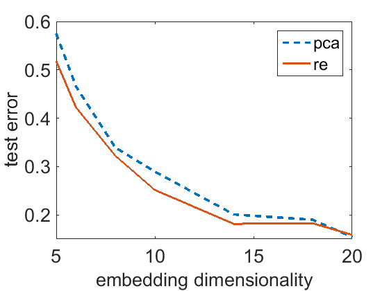
(a) Performance of logistic regression on ALOI when combined with either a feature embedding (PCA) or label embedding (RE).

(b) The empirical label covariance spectrum for LSHTC.

At $k=50$, there is no difference in quality between using the Rembrandt (label) embedding and the PCA (feature) embedding. This is not surprising considering the effective rank of the covariance matrix of ALOI is 70. For small embedding dimensionalities, however, PCA underperforms Rembrandt as indicated in Figure 1(a). For larger numbers of output classes, where the embedding dimension will be a small fraction of the number of classes by computational necessity, we anticipate PCA regression will not be competitive.

Note that, in addition to better statistical performance, all of the “embedding + LR” approaches have lower space complexity $O(k(c+d))$ than direct logistic regression $O(cd)$. For ALOI the savings are modest (255600 bytes vs. 516000 bytes) because the input dimensionality is only $d=128$, but for larger problems the space savings are necessary for feasible implementation on a single commodity computer. Inference time on ALOI is identical for embedding and direct approaches in practice (both achieving $\approx 170$k examples/sec).

4.2 ODP

The Open Directory Project [13] is a public human-edited directory of the web which was processed by [6] into a multiclass data set. For these experiments we will consider test classification error utilizing the same train-test split, features, and labels from [8]. Specifically there is a fixed train-test split of 2:1 for all experiments, the representation of document is a bag of words, and the unique class assignment for each document is the most specific category associated with the document.

The procedures are the same as in the previous experiment, except that we do not compare to OAA or full logistic regression due to intractability on a single machine.

Table 3: ODP results. $k=300$ for all embedding strategies.

Method	RE + LR	CS + LR	PCA + LR	LT
Test Error	83.15%	85.14%	90.37%	93.46%

The combination of Rembrandt and logistic regression result is, to the best of our knowledge, the best published result on this dataset. PCA logistic regression has a performance gap compared to Rembrandt and logistic regression. The poor performance of PCA logistic regression is doubly unsurprising, both for general reasons previously discussed, and due to the fact that covariance matrices of text data typically have a long plateau of weak spectral decay. In other words, for text problems projection dimensions quickly become nearly equivalent in terms of input reconstruction error, and common words and word combinations are not discriminative. In contrast, Rembrandt leverages the spectral properties of the prediction covariance of equation (3), rather than the spectral properties of the input features.

Finally, we remark the following: although inference (i.e., finding the maximum output) is linear in the number of classes, the constant factors are favorable due to modern vectorized processors, and therefore proceeds at $\approx 1700$ examples/sec for the embedding based approaches.

4.3 LSHTC

The Large Scale Hierarchical Text Classification Challenge (version 4) was a public competition involving multilabel classification of documents into approximately 300,000 categories [24]. The training and test files are available from the Kaggle platform. The features are bag of words representations of each document.

4.3.1 Embedding Quality Assessment

Table 4: Embedding quality for LSHTC. $k=100$ for all embedding strategies.

Method	Most fraternal	CS	PLST	Rembrandt
Sibling Fraction	0.32%	3.08%	19.65%	23.61%

A representation of a DAG hierarchy associated with the classes is also available. We used this to assess the quality of various embedding strategies independent of classification performance. In particular, we computed the fraction of class embeddings whose nearest neighbor was also a sibling in the DAG, as shown in Table 4. “Most fraternal” refers to an embedding which arranges for every category’s nearest neighbor in the embedding to be the node in the DAG with the most siblings, i.e., the constant predictor baseline for this task. PLST [42] has performance close to Rembrandt according to this metric, so the 3.2 average nonzero classes per example is apparently enough for the approximation underlying PLST to be reasonable.

4.3.2 Empirical Label Covariance Spectrum

Our embedding approach is based upon a low-rank assumption for the (unobservable) prediction covariance of equation (3). Because LSHTC is a multi-label dataset, we can use the empirical label covariance as a proxy to investigate the spectral properties of the prediction covariance and test our assumption. We used Algorithm 1 (i.e., two pass randomized PCA) to estimate the spectrum of the empirical label covariance, shown in Figure 1(b). The spectrum decays modestly and suggests that an embedding dimension of $k\approx 1000$ or more might be necessary for good classification performance.

4.3.3 Classification Performance

We built an end-to-end classifier using an approximate kernelized variant of Algorithm 3, where we processed the embeddings with Random Fourier Features [37], i.e., in line 5 of Algorithm 3 we use a random cosine feature map for $\phi$. We found Cauchy distributed random vectors, corresponding to the Laplacian kernel, gave good results. We used 4,000 random features and tuned the kernel bandwidth via cross-validation on the training set.

The LSHTC competition metric is macro-averaged F1, which emphasizes performance on rare classes. However, we are using a multilabel classification algorithm which maximizes accuracy of predictions without regard to the importance of rare classes. Therefore we compare with published results of [36], who report example-averaged precision-at-$k$ on the label ordering induced for each example. To facilitate comparison we do a 75:25 train-test split of the public training set, which is the same proportions as in their experiments (albeit a different split).

Based upon the previous spectral analysis, we anticipate a large embedding dimension is required for best results. With our current implementation, up to the limit of available memory in our desktop machine ($k=800$) we found increasing embedding dimensionality improved performance.

Table 5: LSHTC results.

Method	RE ($k=800$) + ILR	RE ($k=500$) + ILR	FastXML	LPSR-NB
Precision-at-1	53.39%	52.84%	49.78%	27.91%

“RE $(k=\ldots)$ + ILR” corresponds for $Rembrandt$ coupled with independent (kernel) logistic regression, i.e., Algorithm 3. LPSR-NB is the Label Partitioning by Sub-linear Ranking algorithm of [46] composed with a Naive Bayes base learner, as reported in [36], where they also introduce and report precision for the multilabel tree learning algorithm FastXML. Inference for our best model proceeds at $\approx$ 60 examples/sec, substantially slower than for ODP, due to the larger output space, larger embedding dimensionality, and the use of random Fourier features.

5 Discussion

In this paper we identify a correspondence between rank constrained regression and label embedding, and we exploit that correspondence along with randomized matrix decomposition techniques to develop a fast label embedding algorithm.

To facilitate analysis and implementation, we focused on linear prediction, which is equivalent to a simple neural network architecture with a single linear hidden layer bottleneck. Because linear predictors perform well for text classification, we obtained excellent experimental results, but more sophistication is required for tasks where deep architectures are state-of-the-art. Although the analysis presented herein would not strictly be applicable, it is plausible that replacing line 6 in Algorithm 2 with an optimization over a deep architecture could yield good embeddings. This would be computationally beneficial as reducing the number of outputs (i.e., predicting embeddings rather than labels) would mitigate space constraints for GPU training.

Our technique leverages the (putative) low-rank structure of the prediction covariance of equation (3). For some problems a low-rank plus sparse assumption might be more appropriate. In such cases combining our technique with L1 regularization, e.g., on a classification residual or on separately regularized direct connections from the original inputs, might yield superior results.

Acknowledgments

We thank John Langford for providing the ALOI and ODP data sets.

References

- [1] Agarwal, A., Kakade, S.M., Karampatziakis, N., Song, L., Valiant, G.: Least squares revisited: Scalable approaches for multi-class prediction. In: Proceedings of The 31st International Conference on Machine Learning. pp. 541–549 (2014)
- [2] Barker, M., Rayens, W.: Partial least squares for discrimination. Journal of chemometrics 17(3), 166–173 (2003)
- [3] Bartlett, M.S.: Further aspects of the theory of multiple regression. In: Mathematical Proceedings of the Cambridge Philosophical Society. vol. 34, pp. 33–40. Cambridge Univ Press (1938)
- [4] Beck, A., Teboulle, M.: A fast iterative shrinkage-thresholding algorithm for linear inverse problems. SIAM Journal on Imaging Sciences 2(1), 183–202 (2009)
- [5] Bengio, S., Weston, J., Grangier, D.: Label embedding trees for large multi-class tasks. In: Advances in Neural Information Processing Systems. pp. 163–171 (2010)
- [6] Bennett, P.N., Nguyen, N.: Refined experts: improving classification in large taxonomies. In: Proceedings of the 32nd international ACM SIGIR conference on Research and development in information retrieval. pp. 11–18. ACM (2009)
- [7] Breiman, L., Friedman, J.H.: Predicting multivariate responses in multiple linear regression. Journal of the Royal Statistical Society: Series B (Statistical Methodology) 59(1), 3–54 (1997)
- [8] Choromanska, A., Langford, J.: Logarithmic time online multiclass prediction. arXiv preprint arXiv:1406.1822 (2014)
- [9] Cissé, M., Artières, T., Gallinari, P.: Learning compact class codes for fast inference in large multi class classification. In: Machine Learning and Knowledge Discovery in Databases, pp. 506–520. Springer (2012)
- [10] DeCoro, C., Barutcuoglu, Z., Fiebrink, R.: Bayesian aggregation for hierarchical genre classification. In: ISMIR. pp. 77–80 (2007)
- [11] Dekel, O., Keshet, J., Singer, Y.: Large margin hierarchical classification. In: Proceedings of the twenty-first international conference on Machine learning. p. 27. ACM (2004)
- [12] Deng, J., Dong, W., Socher, R., Li, L.J., Li, K., Fei-Fei, L.: Imagenet: A large-scale hierarchical image database. In: Computer Vision and Pattern Recognition, 2009. CVPR 2009. IEEE Conference on. pp. 248–255. IEEE (2009)
- [13] DMOZ: The open directory project (2014), http://dmoz.org/
- [14] Friedland, S., Torokhti, A.: Generalized rank-constrained matrix approximations. SIAM Journal on Matrix Analysis and Applications 29(2), 656–659 (2007)
- [15] Frome, A., Corrado, G.S., Shlens, J., Bengio, S., Dean, J., Mikolov, T., et al.: Devise: A deep visual-semantic embedding model. In: Advances in Neural Information Processing Systems. pp. 2121–2129 (2013)
- [16] Geladi, P., Kowalski, B.R.: Partial least-squares regression: a tutorial. Analytica chimica acta 185, 1–17 (1986)
- [17] Geusebroek, J.M., Burghouts, G.J., Smeulders, A.W.: The Amsterdam library of object images. International Journal of Computer Vision 61(1), 103–112 (2005)
- [18] Gopal, S., Yang, Y.: Recursive regularization for large-scale classification with hierarchical and graphical dependencies. In: Proceedings of the 19th ACM SIGKDD international conference on Knowledge discovery and data mining. pp. 257–265. ACM (2013)
- [19] Halko, N., Martinsson, P.G., Tropp, J.A.: Finding structure with randomness: Probabilistic algorithms for constructing approximate matrix decompositions. SIAM review 53(2), 217–288 (2011)
- [20] Hotelling, H.: Relations between two sets of variates. Biometrika pp. 321–377 (1936)
- [21] Hsu, D., Kakade, S., Langford, J., Zhang, T.: Multi-label prediction via compressed sensing. In: NIPS. vol. 22, pp. 772–780 (2009)
- [22] Izenman, A.J.: Reduced-rank regression for the multivariate linear model. Journal of multivariate analysis 5(2), 248–264 (1975)
- [23] Jégou, H., Douze, M., Schmid, C.: On the burstiness of visual elements. In: Computer Vision and Pattern Recognition, 2009. CVPR 2009. IEEE Conference on. pp. 1169–1176. IEEE (2009)
- [24] Kaggle: Large scale hierarchical text classification (2014), http://www.kaggle.com/c/lshtc
- [25] Kosmopoulos, A., Gaussier, E., Paliouras, G., Aseervatham, S.: The ECIR 2010 large scale hierarchical classification workshop. In: ACM SIGIR Forum. vol. 44, pp. 23–32. ACM (2010)
- [26] Langford, J.: Vowpal Wabbit. https://github.com/JohnLangford/vowpal_wabbit/wiki (2007)
- [27] Lebret, R., Collobert, R.: Word emdeddings through hellinger pca. arXiv preprint arXiv:1312.5542 (2013)
- [28] Liberty, E.: Simple and deterministic matrix sketching. In: Proceedings of the 19th ACM SIGKDD international conference on Knowledge discovery and data mining. pp. 581–588. ACM (2013)
- [29] Lokhorst, J.: The lasso and generalised linear models. Tech. rep., University of Adelaide, Adelaide (1999)
- [30] Lu, Y., Foster, D.P.: Large scale canonical correlation analysis with iterative least squares. arXiv preprint arXiv:1407.4508 (2014)
- [31] Mikolov, T., Chen, K., Corrado, G., Dean, J.: Efficient estimation of word representations in vector space. arXiv preprint arXiv:1301.3781 (2013)
- [32] Mineiro, P.: randembed. https://github.com/pmineiro/randembed (2015)
- [33] Mineiro, P., Karampatziakis, N.: A randomized algorithm for CCA. arXiv preprint arXiv:1411.3409 (2014)
- [34] Nesterov, Y.: A method of solving a convex programming problem with convergence rate . Dokl. Akad. Nauk SSSR 269, 543–547 (1983)
- [35] Palatucci, M., Pomerleau, D., Hinton, G.E., Mitchell, T.M.: Zero-shot learning with semantic output codes. In: Advances in neural information processing systems. pp. 1410–1418 (2009)
- [36] Prabhu, Y., Varma, M.: Fastxml: a fast, accurate and stable tree-classifier for extreme multi-label learning. In: Proceedings of the 20th ACM SIGKDD international conference on Knowledge discovery and data mining. pp. 263–272. ACM (2014)
- [37] Rahimi, A., Recht, B.: Random features for large-scale kernel machines. In: Advances in neural information processing systems. pp. 1177–1184 (2007)
- [38] Rao, C.R.: The utilization of multiple measurements in problems of biological classification. Journal of the Royal Statistical Society. Series B (Methodological) 10(2), pp. 159–203 (1948), http://www.jstor.org/stable/2983775
- [39] Schietgat, L., Vens, C., Struyf, J., Blockeel, H., Kocev, D., Džeroski, S.: Predicting gene function using hierarchical multi-label decision tree ensembles. BMC Bioinformatics 11, 2 (2010)
- [40] Socher, R., Ganjoo, M., Manning, C.D., Ng, A.: Zero-shot learning through cross-modal transfer. In: Advances in Neural Information Processing Systems. pp. 935–943 (2013)
- [41] Sun, L., Ji, S., Yu, S., Ye, J.: On the equivalence between canonical correlation analysis and orthonormalized partial least squares. In: IJCAI. vol. 9, pp. 1230–1235 (2009)
- [42] Tai, F., Lin, H.T.: Multilabel classification with principal label space transformation. Neural Computation 24(9), 2508–2542 (2012)
- [43] Wang, H., Ding, C., Huang, H.: Multi-label linear discriminant analysis. In: Computer Vision–ECCV 2010, pp. 126–139. Springer (2010)
- [44] Weinberger, K.Q., Chapelle, O.: Large margin taxonomy embedding for document categorization. In: Advances in Neural Information Processing Systems. pp. 1737–1744 (2009)
- [45] Weston, J., Bengio, S., Usunier, N.: Wsabie: Scaling up to large vocabulary image annotation. In: IJCAI. vol. 11, pp. 2764–2770 (2011)
- [46] Weston, J., Makadia, A., Yee, H.: Label partitioning for sublinear ranking. In: Proceedings of the 30th International Conference on Machine Learning (ICML-13). pp. 181–189 (2013)