The superconformal index of theories of class $\SS$

Abstract

We review different aspects of the superconformal index of ${\cal N}=2$ superconformal theories of class ${\cal S}$. In particular we discuss the relation of the index of class ${\cal S}$ theories to topological QFTs and integrable models, and review how this relation can be harnessed to completely determine the index.

This is part of a combined review on $2d$-$4d$ relations, edited by J. Teschner.

1 Introduction

This volume surveys the $4d/2d$ relations that arise in the study of class ${\cal S}$, the set of four-dimensional ${\cal N}=2$ supersymmetric field theories obtained by compactification of a six-dimensional $(2,0)$ theory on a punctured Riemann surface ${\cal C}$. There is an extensive $4d/2d$ dictionary relating several protected observables of the four-dimensional theory ${T}[{\cal C}]$ to observables of certain natural theories defined on the associated surface ${\cal C}$. In this chapter we focus on the superconformal index of ${T}[{\cal C}]$ and on its re-interpretation as a topological quantum field theory (TQFT) living on ${\cal C}$. We shall restrict our discussion to the subset of theories that enjoy conformal invariance, for which the general index is well-defined.

The superconformal index, or index for short, encodes some detailed information about the protected spectrum of a superconformal field theory. By construction, it is invariant under exactly marginal deformations of the SCFT. A basic item of the $4d/2d$ dictionary equates the conformal manifold of ${T}[{\cal C}]$ (i.e., the space of its exactly marginal gauge couplings) with the complex structure moduli of ${\cal C}$. We should then expect on general grounds that the index is computed by a TQFT living on ${\cal C}$. A concrete description of this TQFT as an explicit $2d$ theory is only available for certain specializations of the general index, in particular the so-called Schur index corresponds to $q$-deformed two-dimensional Yang-Mills theory in the zero-area limit. The TQFT viewpoint is however very fruitful also in the general case. As different TQFT correlators compute the indices of different $4d$ theories, we are led to study consistency conditions in theory space. This turns out to be a very effective strategy, which allows for the complete determination of the general index for theories of class ${\cal S}$.

2 The superconformal index

Let us introduce the main character of this review. To a superconformal field theory in $d$ space-time dimensions one can associate its superconformal index Romelsberger:2005eg ; Kinney:2005ej , which is nothing but the Witten index of the theory in radial quantization, refined to keep track of a maximal set of commuting conserved quantum numbers $\{C_{i}\}$,

$${\cal I}(\mu_{i})=\mathrm{Tr}\,(-1)^{F}\prod_{i}\mu_{i}^{C_{i}}\,e^{-\beta\delta}\,,\quad\delta\colonequals\{{\cal Q}\,,{\cal Q}^{\dagger}\}\,.$$ (2.1)

The trace is taken over the Hilbert space of the radially quantized theory on $\mathbb{S}^{d-1}$, $F$ is the fermion number and ${\cal Q}$ a chosen Poincaré supercharge. In a given theory, the index is thus a function of the “fugacities” $\{\mu_{i}\}$ that couple to the conserved charges $\{C_{i}\}$. The conserved charges are chosen as to commute with each other, with the chosen supercharge ${\cal Q}$ and with its conjugate (conformal) supercharge ${\cal Q}^{\dagger}$. If the theory is unitary, which we shall always assume, then $\delta\colonequals\{{\cal Q}\,,{\cal Q}^{\dagger}\}\geqslant 0$. By a familiar argument, the index counts (with signs) cohomology classes of ${\cal Q}$. Indeed the Hilbert space decomposes into the subspace of states with $\delta=0$, which are automatically killed by both ${\cal Q}$ and ${\cal Q}^{\dagger}$ (these are the “harmonic representatives” of the cohomology classes), and the subspace with $\delta\neq 0$, where one can choose a basis such that all states belong to a pair $(\psi,{\cal Q}\psi)$, with ${\cal Q}^{\dagger}\psi=0$. The paired states have the same charges $\{C_{i}\}$ but opposite statistics, so their combined contribution to the trace vanishes. Since the trace in (2.1) receives contributions only from the harmonic representatives, the index is in fact independent of $\beta$. The states with $\delta=0$ are annihilated by some of the supercharges and as such they belong to shortened representation of the superconformal algebra.

As the energy (conformal dimension) of a generic long multiplet of the superconformal algebra is lowered to the unitarity bound, the long multiplet breaks up into a direct sum of short multiplets, containing states with $\delta=0$, but by continuity their total contribution to the index is zero. So even within the $\delta=0$ subspace there may be fermion/boson cancellations between states with the same charges $\{C_{i}\}$, associated to recombinations of short multiplets into long ones. In fact one can equivalently characterize the index as the most general invariant that counts short multiplets, up to the equivalence relation setting to zero combinations of short multiplets that have the right quantum numbers to recombine into long ones Kinney:2005ej . It follows, at least formally, that the index is invariant under changes of continuous parameters of the theory preserving superconformal invariance, i.e. it is constant over the conformal manifold of the theory. As the exactly marginal couplings are varied, long multiplets may split into short ones or short multiplets recombine into long ones, but this is immaterial for the index. In other contexts, the formal independence of supersymmetric indices on continuous parameters is known to fail, leading to rich wall-crossing phenomena. In our case, however, we are dealing with theories that have a discrete spectrum of states, and such that the subspaces with fixed values of the quantum numbers $\{C_{i}\}$ are finite-dimensional, so the formal argument is completely rigorous. The index is thus truly invariant under exactly marginal deformations preserving the full superconformal algebra of the model.

The superconformal index can be defined for theories in various spacetime dimensions, and with different amounts of superconformal symmetry. We have given the “Hamiltonian” definition in terms of a trace formula, but the index has an equivalent “Lagrangian” interpretation as a supersymmetric partition function on $\mathbb{S}^{d-1}\times\mathbb{S}^{1}$, with twisted boundary conditions around the “temporal” $\mathbb{S}^{1}$ to incorporate the dependence on the various fugacities. See [V:5] in this volume for more details on this approach. Viewed as a partition function, the index makes sense for non-conformal theories, though in those cases it should be more properly referred to as a supersymmetric index. One can show that such a partition function is independent on the RG scale, so that the superconformal index of a theory realized as the IR fixed point of some RG flow can be often computed using the non-conformal UV starting point of the flow Romelsberger:2005eg ; Romelsberger:2007ec ; Festuccia:2011ws . Examples where this is a very useful strategy include ${\cal N}=1$ gauge theories in four dimensions, and susy gauge theories in three and two dimensions. The partition function interpretation is also useful to obtain the index in the presence of various BPS defects, by the techniques of supersymmetric localization. In this review we will mostly stick to the trace interpretation of the index, and localization will not play a role. We will determine the index of the ${\cal N}=2$ SCFTs of class ${\cal S}$ (even in the presence of certain BPS defects) by a more abstract algebraic viewpoint. A direct localization approach would not be an option since these theories do not generally admit a known Lagrangian description.

We now specialize to the case of interest, namely ${\cal N}=2$ superconformal theories in four dimensions. The ${\cal N}=2$ superconformal index depends on three superconformal fugacities $(p,q,t)$ and on any number of fugacities $\{a_{i}\}$ associated to flavor symmetries (which, by definition, commute with the superconformal algebra),

$${\cal I}(p,q,t;a_{i})\colonequals\mathrm{Tr}(-1)^{F}\,\left(\frac{t}{pq}\right)^{r}\,p^{j_{12}}\,q^{j_{34}}\,t^{R}\,\prod_{i}a_{i}^{f_{i}}\,e^{-\beta\delta_{2\dot{-}}}\,,$$ (2.2)

where

$$2\delta_{2\dot{-}}\colonequals\{\widetilde{\cal Q}_{2\dot{-}},\,\widetilde{\cal Q}_{2\dot{-}}^{\dagger}\}=E-2j_{2}-2R+r\,.$$ (2.3)

We will always assume that

$$|p|<1\,,\qquad|q|<1\,,\qquad|t|<1\,,\qquad|a_{i}|=1\,,\qquad\left|\frac{p\,q}{t}\right|<1\,.$$ (2.4)

Our notations are as follows. We denote by $E$ the conformal hamiltonian (dilatation generator), by $j_{1}$ and $j_{2}$ the Cartan generators of of the $SU(2)_{1}\times SU(2)_{2}$ isometry group of ${\mathbb{S}}^{3}$, by $R$ and $r$ the Cartan generators of the $SU(2)_{R}\times U(1)_{r}$ the superconformal R-symmetry. We have also defined $j_{12}\colonequals j_{2}-j_{1}$ and $j_{34}\colonequals j_{2}+j_{1}$, which generate rotations in two orthogonal planes (thinking of ${\mathbb{S}}^{3}$ as embedded in ${\mathbb{R}}^{4}$). Finally $\{f_{i}\}$ are the flavor symmetry generators. In our conventions, we label the supercharges as

$${\cal Q}^{\cal I}_{\alpha}\,\qquad\tilde{\cal Q}_{{\cal I}\dot{\alpha}}\,\qquad{\cal S}_{\cal I}^{\alpha}\,\qquad\tilde{\cal S}^{{\cal I}\dot{\alpha}}\,,$$ (2.5)

where $\alpha=\pm$ is an $SU(2)_{1}$ index, $\dot{\alpha}=\dot{\pm}$ an $SU(2)_{2}$ index and ${\cal I}=1,2$ an $SU(2)_{R}$ index. We have ${\cal S}={{\cal Q}}^{\dagger}$ and $\tilde{\cal S}={\tilde{\cal Q}}^{\dagger}$. Writing an explicit trace formula for the index involves a choice of supercharge. With no loss of generality, we chose in  (2.2) to count cohomology classes of $\tilde{\cal Q}_{2\dot{-}}$, which has quantum numbers $E=R=-r=\frac{1}{2}$, $(j_{1},j_{2})=(0,-\frac{1}{2})$. The states that to this index are the “harmonic representatives” satisfy $\delta\equiv\delta_{2\dot{-}}=0$. All other choices of a Poincaré supercharge would give an equivalent index Kinney:2005ej .

In appendix B we review the shortening conditions of the ${\cal N}=2$ superconformal algebra and the recombination rules of short multiplets into long ones. Explicit formulae for the index of individual short multiplets are given in appendix B of Gadde:2011uv and will not be repeated here. It is important to keep in mind that knowledge of the index alone is in general not sufficient to completely reconstruct the spectrum of short representations of a given theory. Schematically, the issue is the following Gadde:2009dj . Suppose that two short multiplets, $S_{1}$ and $S_{2}$, can recombine to form a long multiplet $L_{1}$,

$$S_{1}\oplus S_{2}=L_{1}\,,$$ (2.6)

and similarly that $S_{2}$ can recombine with a third short multiplet $S_{3}$ to give another long multiplet $L_{2}$,

$$S_{2}\oplus S_{3}=L_{2}\,.$$ (2.7)

By construction, the index evaluates to zero on long multiplets, so

$$\mathcal{I}(S_{1})=-\mathcal{I}(S_{2})=\mathcal{I}(S_{3})\,.$$ (2.8)

The index cannot distinguish between the two multiplets $S_{1}$ and $S_{3}$. (Note that $S_{2}$ is distinguished from $S_{1}\sim S_{3}$ by the overall sign.) A detailed discussion of equivalence classes of multiplets that have the same ${\cal N}=2$ superconformal index can be found in section 5.2 of Gadde:2009dj .

2.1 Free field combinatorics

The simplest examples of conformal quantum field theories are free theories. In a free theory, the general local operator is obtained from normal ordering of the elementary fields, and its quantum numbers including the conformal dimension take their classical “engineering” values. By the state/operator map, local operators inserted at the origin are in one-to-one correspondence with states. Enumerating states reduces then to the simple combinatorial problem of enumerating all possible composite “words” (or “multi-particles”) built out of the elementary “letters” (or “single-particles”), which are the elementary fields and their space-time derivatives.

For our purposes, we are interested in enumerating states with $\delta=0$, and since in a free theory the value of $\delta$ of a composite operator is simply the sum of the values of $\delta$ of its elementary letters, we may from the start restrict to the letters with $\delta=0$. The letters contributing the index of the free ${\cal N}=2$ hypermultiplet and of the free vector multiplet ${\cal N}=2$ are shown in Table 1. One immediately finds the following single-particle indices (i.e., the indices computed over the set of single-particle states):

$${\cal I}^{s.p.}_{H}=t^{\frac{1}{2}}\,\frac{1-\frac{p\,q}{t}}{(1-p)(1-q)}(a+a^{-1})\,\chi_{\Lambda}(\bf x)\,,$$ (2.9)

$${\cal I}^{s.p.}_{V}=-\frac{q}{1-q}-\frac{p}{1-p}+\frac{\frac{p\,q}{t}-t}{(1-p)(1-q)}\,.$$ (2.10)

Here $a$ is a $U(1)$ fugacity under which the two half-hypers have opposite charges and $\chi_{\Lambda}(\bf x)$ is the character of the representation of some global symmetry. The multi particle-indices are given by the plethystic exponentials of the single-particle ones. In particular the index of a free hypermultiplet in a bi-fundamental representation of $SU(n)\times SU(n)$, which will play an important role in our discussion, is given by

$${\cal I}_{H}(a,{\bf x},{\bf y};p,q,t) = {\rm PE}\left[t^{\frac{1}{2}}\,\frac{1-\frac{p\,q}{t}}{(1-p)(1-q)}(a+a^{-1})\left(\sum_{i=1}^{n}x_{i}\right)\left(\sum_{j=1}^{n}y_{j}\right)\right]$$ (2.11)

$$= \prod_{i,j=1}^{n}\Gamma(t^{\frac{1}{2}}\,a\,x_{i}\,y_{j}\,;\,p,\,q)\,\Gamma(t^{\frac{1}{2}}\,(a\,x_{i}\,y_{j})^{-1};\,p,\,q)\,.$$

We collect the definitions of the plethystic exponenential, elliptic Gamma function, and related objects in appendix A.

Letters	$E$	$j_{1}$	$j_{2}$	$R$	$r$	$\mathcal{I}(p,q,t)$
$\phi$	$1$	$0$	$0$	$0$	$-1$	$pq/t$
$\lambda^{1}_{\pm}$	$\frac{3}{2}$	$\pm\frac{1}{2}$	$0$	$\frac{1}{2}$	$-\frac{1}{2}$	$-p$, $-q$
$\bar{\lambda}_{2\dot{+}}$	$\frac{3}{2}$	$0$	$\frac{1}{2}$	$\frac{1}{2}$	$\frac{1}{2}$	$-t$
$\bar{F}_{\dot{+}\dot{+}}$	$2$	$0$	$1$	$0$	$0$	$pq$
$\partial_{-\dot{+}}\lambda^{1}_{+}+\partial_{+\dot{+}}\lambda^{1}_{-}=0$	$\frac{5}{2}$	$0$	$\frac{1}{2}$	$\frac{1}{2}$	$-\frac{1}{2}$	$pq$
$Q$	$1$	$0$	$0$	$\frac{1}{2}$	$0$	$\sqrt{t}$
$\bar{\psi}_{\dot{+}}$	$\frac{3}{2}$	$0$	$\frac{1}{2}$	$0$	$-\frac{1}{2}$	$-pq/\sqrt{t}$
$\partial_{\pm\dot{+}}$	$1$	$\pm\frac{1}{2}$	$\frac{1}{2}$	$0$	$0$	$p$, $q$

Table 1: Contributions to the index from single-particle (letter) operators of the two basic ${\cal N}=2$ multiplets: the vector multiplet and the hypermultiplet. We denote by $(\phi,\bar{\phi},\lambda^{\cal I}_{\alpha},\bar{\lambda}_{{\cal I}\,\dot{\alpha}},F_{\alpha\beta},\bar{F}_{\dot{\alpha}\dot{\beta}})$ the components of the adjoint ${\cal N}=2$ vector multiplet, by $(Q,\bar{Q},\psi_{\alpha},\bar{\psi}_{\dot{\alpha}})$ the components of the ${\cal N}=1$ chiral multiplet, and by $\partial_{\alpha\dot{\alpha}}$ the spacetime derivatives.

Conversely, one of the hallmarks of a free theory is the fact that the plethystic log of the index is simple. For example, formally analogous to the counting problem in free field theory is the counting problem for large $N$ theories. It often happens that the conformal gauge theories come in families labeled by the rank of the gauge group and in the limit of large rank they have a dual description in terms of supergravity in $AdS$ backgrounds Kinney:2005ej . In such cases the operators counted by the index are dual to free supergravity modes. Thus, taking the limit of large $N$ the index reduces again to a simple plethystic exponential of the towers of single trace operators dual to the finite number of free supergravity fields.

2.2 Gauging

After we dealt with free theories, let us turn to interacting models. In general, we should not expect any simple combinatorial description of the set of local operators in an interacting theory. An important exception are the superconformal field theories that admit a Lagrangian description, which by definition are continuously connected to free field theories by turning off the gauge couplings. Since the index is independent of exactly marginal deformations, we may as well compute it in the free limit (setting to zero all gauge couplings). The only effect of the gauging is the Gauss law constraint, i.e. the projection onto gauge invariant states.

More generally, starting from a SCFT ${\cal T}$, we can obtain a new superconformal field theory ${\cal T}_{G}$ by gauging a subgroup $G$ of the flavor symmetry of ${\cal T}$, provided of course that the gauge coupling beta functions vanish. If the index of ${\cal T}$ is known, we find the index of ${\cal T}_{G}$ by multiplying by the index of a vector multiplet in the adjoint representation of $G$, and then integrating over $G$ with the invariant Haar measure to enforce the projecting over gauge singlets,

$${\cal I}[{\cal T}_{G}]=\int[d{\bf z}]_{G}\;{\cal I}_{V}({\bf z})\;{\cal I}[{\cal T}]({\bf z})\,.$$ (2.12)

In fact we can treat the index ${\cal I}_{{\cal T}}({\bf z})$ as a “black-box”: it might be the index of a collection of free hypermultiplets, the index of a gauge theory, or the index of an interacting theory for which we do not know a useful description in terms of a Lagrangian. Whenever a flavor symmetry is gauged in four dimensions, the effect on the index is simply to introduce the vector multiplet and project onto gauge-invariant states.

In all known examples, conformal manifolds of ${\cal N}=2$ SCFTs are parametrized by gauge couplings. It is tempting to speculate that the most general ${\cal N}=2$ SCFT is obtained by gauging a set of elementary building blocks, each of which is an isolated theory with no exactly marginal couplings. The simplest of such an elementary building block is the free hypermultplet theory. We will encounter below several other examples of building blocks with no known Lagrangian description. Determining the index of such isolated theories would appear to be very challenging. Fortunately, for theories of class ${\cal S}$ we can leverage the additional structure of generalized S-duality. Let us turn to a concrete illustration.

3 Interlude: duality and the index of $E_{6}$ SCFT

In this section, we will sketch how to determine the index of a canonical example of isolated non-Lagrangian theory, the SCFT with $E_{6}$ flavor symmetry of Minahan and Nemeschansky Minahan:1996fg . The general idea is to couple the isolated theory to some extra stuff, and use dualities to relate the larger theory to a more tractable model.

For the case at hand, we exploit Argyres-Seiberg duality argyres-2007-0712 . On one side of the duality we have an $SU(3)$ SYM with $N_{f}=6$ flavors. On the other side of the duality we have a hypermultiplet in the fundamental representation of gauged $SU(2)$ under which also a strongly-coupled theory with $E_{6}$ flavor symmetry Minahan:1996fg is charged. The $SU(2)$ gauged group is a sub-group of the $E_{6}$ flavor symmetry. By the rules of computing the index reviewed in the previous section, this duality can be written as equality of two integrals Gadde:2010te ,

$$\int[d{\bf z}]_{G=SU(3)}\,{\cal I}^{SU(3)}_{V}({\bf z})\,{\cal I}^{(1)}_{H}({\bf z},{\bf y},{\bf x},a,b)=$$ (3.1)

$$\qquad\qquad\qquad\int[d{z}]_{G=SU(2)}\,{\cal I}^{SU(2)}_{V}(z)\,{\cal I}^{(2)}_{H}(z,(a/b)^{3/2})\,{\cal I}_{E_{6}}({\bf x},{\bf y},\{z(ab)^{-\frac{1}{2}},z^{-1}(ab)^{-\frac{1}{2}}\})\,.$$

Here ${\cal I}_{E_{6}}({\bf x}_{1},{\bf x}_{2},{\bf x}_{3})$ is the unkown index of the theory with $E_{6}$ flavor symmetry with $\{{\bf x}_{i}\}$ being the fugacities for $SU(3)^{3}$ maximal subgroup of $E_{6}$; ${\bf y}$ and ${\bf x}$ are $SU(3)$ fugacities and $a,b$ are two $U(1)$ fugacities. The quantity ${\cal I}^{(1)}_{H}({\bf z},{\bf y},{\bf x},a,b)$ represents the index of a collection of hypermultiplets in the bi-fundamental representation of flavor of $SU(3)^{2}$ and the gauged $SU(3)$, whereas ${\cal I}^{(2)}_{H}(z,(a/b)^{3/2})$ is a fundamental hypermultiplet of $SU(2)$. The powers of $U(1)$ fugacities $a$ and $b$ on the right-hand side of the equality are a consequence of the details of the map of global symmetries between the two duality frames. In general from equalities of integrals of this sort one cannot extract the precise values of the integrands. However, in this particular case the integral on the right-hand side is invertible and just by assuming the Argyres-Seiberg duality as manifested for the index in (3.1) one can explicitly deduce the index ${\cal I}_{E_{6}}$. Schematically, this inversion procedure takes the following form

$${\cal I}_{E_{6}}({\bf x},{\bf y},\{c(ab)^{-\frac{1}{2}},c^{-1}(ab)^{-\frac{1}{2}}\})=\oint_{\cal C}\frac{d\,h}{2\pi ih}\Delta(h,c)\,\int[d{\bf z}]_{G=SU(3)}\,{\cal I}^{SU(3)}_{V}({\bf z})\,{\cal I}^{(1)}_{H}({\bf z},{\bf y},{\bf x},a,b)\,.\\$$

Here ${\cal C}$ is a well-defined integration contour and $\Delta$ is a specific inversion kernel spirinv . Physically, the fact that the integral is invertible means that the extra hyper-multiplet introduced while gauging a sub-group of the $E_{6}$ symmetry adds enough structure so that the information about the protected spectrum of the $E_{6}$ theory itself, a-priori lost after gauging, can be still recovered.

We thus are able to completely fix the superconformal index of a theory not connected to a free theory by a continuous parameter. The trick is to enlarge the theory with the bigger theory admitting an alternative description which can be connected to a free theory by continuous deformation. This basic idea will be behind the general procedure we will outline in the next sections.

Before turning to the general discussion of class ${\cal S}$ theories, let us illustrate in this concrete example what kind of physical information can be extracted from the index. Explicitly computing (3) one obtains to the lowest orders in the series expansion in fugacities

$${\cal I}_{E_{6}} = PE[{\cal I}_{u}]\,PE[{\cal I}_{H}(\chi_{78})]\,PE[{\cal I}_{T}]\;\times$$

$$\qquad\left(1-(t^{2}-p\,q\,t+t^{2}(p+q))\,(\chi_{650}+1)-\frac{p^{3}q^{3}}{t^{2}}+p\,q\,t\,\chi_{78}+\cdots\right)\,.$$

In the first line we have the protected multiplets appearing in this theory: ${\cal I}_{u}$ is the Coulomb branch multiplet (the dual of $u=Tr\phi^{3}$ of the $SU(3)$ gauge theory), ${\cal I}_{H}$ is the Higgs branch generator, $X$, in ${\bf 78}$ of the $E_{6}$ global symmetry, and ${\cal I}_{T}$ is the stress-energy multiplet. The quantum numbers of these multiplets are different from free fields. Moreover, on the second line we have constraints appearing removing some of the contributions generated on the first line: these constraints are the footprint of the non-trivial dynamics of the theory. For example one constraint encoded here is

$$\left[X\otimes X\right]_{650\oplus 1}=0\,,$$ (3.3)

which is the Joseph’s relation discussed in Gaiotto:2008nz .

4 Derivation of the index for theories of class ${\cal S}$

In this section we will determine the index for all theories of class ${\cal S}$. Broadly speaking, we will be using the same kind of physical input as in the previous section, namely knowledge of the index for Lagrangian theories and the assumption of generalized S-duality. We will however exploit these ingredients in a different way, arriving at a particularly elegant and uniform description of the general index. For simplicity we focus on the basic index (the ${\mathbb{S}}^{3}\times{\mathbb{S}}^{1}$ partition function), and to the simplest class ${\cal S}$ theories of type $A$. Several generalizations will be mentioned in section 6.

4.1 Class ${\cal S}$

A lightening review of class ${\cal S}$ is in order. A $4d$ superconformal field theory of class ${\cal S}$ is specified the following data:

• A choice of the type $\mathfrak{g}$ of the $(2,0)$ theory, where $\mathfrak{g}=\{A_{n},D_{n},E_{6},E_{7},E_{8}\}$ is a simply-laced Lie algebra.

• A choice of UV curve ${\cal C}_{g,s}$, where $g$ indicates the genus and $s$ the number of punctures of the curve. Only the complex structure moduli of ${\cal C}_{g,s}$ matter. They are interpreted as the exactly marginal gauge couplings of the $4d$ SCFT.

• Each puncture corresponds to a codimension two defect of the $(2,0)$ theory. We restrict to the so-called regular defects, which are labelled by a choice of embedding $\Lambda:\mathfrak{su}(2)\to\mathfrak{g}$. The centralizer $\mathfrak{h}\subset\mathfrak{g}$ of the image of $\Lambda$ in $\mathfrak{g}$ is the flavor symmetry associated to the defect. All in all, the theory enjoys at least the flavor symmetry algebra $\oplus_{i=1}^{s}\mathfrak{h}_{i}$.

We will label the corresponding $4d$ SCFT as ${T}[\mathfrak{g};{\cal C}_{g,s};\{\Lambda_{i}\}]$.

From now on we will restrict our discussion to class ${\cal S}$ theories of type $A$, $\mathfrak{g}=A_{n-1}$. The embeddings $\Lambda:{\mathfrak{su}(2)}\to\mathfrak{su}(n)$ are in one-to-one correspondence with partitions of $n$, $[n_{1}^{\ell_{1}},n_{2}^{\ell_{2}},\dots n_{k}^{\ell_{k}}]$ with $\sum_{i}\ell_{i}n_{i}=n$ and $n_{i}>n_{i+1}$, which indicate how the fundamental representation of $\mathfrak{su}(n)$ decomposes under representations of $\Lambda(\mathfrak{su}(2))$. For the trivial embedding $\Lambda=0$, associated to the partition $[1^{n}]$, we have maximal flavor symmetry $\mathfrak{h}=\mathfrak{su}(n)$ and the corresponding puncture is called maximal. The other extreme case case is the principal embedding, associated to the partition $[n]$, leading to $\mathfrak{h}=0$ (no flavor symmetry), so the puncture is effectively deleted. Another important case is the subregular embedding, associated to the partition $[n-1,1]$, which leads to $\mathfrak{h}=\mathfrak{u}(1)$, the smallest non-trivial flavor symmetry, so the corresponding puncture is called a minimal puncture.

The surface ${\cal C}_{g,s}$ can be assembled by gluing together three-punctured spheres, or “pairs of pants” (viewed as three-vertices) and cylinders (viewed as propagators). Each cylinder is associated to a simple gauge group factor of the $4d$ SCFT, with the plumbing parameter interpreted as the corresponding marginal gauge coupling. The degeneration limit of the surface where one cylinder becomes very long corresponds to the weak coupling limit of that gauge group. Cutting a cylinder is interpreted as “ungauging” an $SU(n)$ gauge group, leaving behind two maximal punctures, each carrying $SU(n)$ flavor symmetry. Conversely, gluing two maximal punctures corresponds to gauging the diagonal subgroup of their $SU(n)\times SU(n)$ flavor symmetry. The basic building blocks of class ${\cal S}$ are thus the theories associated to three-punctured spheres, $T_{n}^{\Lambda_{1},\Lambda_{2},\Lambda_{3}}\colonequals{T}[\mathfrak{su}(n);{\cal C}_{0,3};\Lambda_{1}\,\Lambda_{2}\,\Lambda_{3}]$. These are isolated SCFTs with no tunable couplings, in harmony with the fact that three-punctured spheres carry no complex structure moduli. Most of them have no known Lagrangian description. An important exception is the theory associated to two maximal and one minimal puncture, $T_{n}^{[1^{n}]\,[1^{n}]\,[n-1,1]}$, which is identified with the free hypermultiplet in the bifundamental representation of $SU(n)\times SU(n)$.

$\Bigm{|}$   $4d$ theory $T[{\cal C}]$	Riemann surface ${\cal C}$ $\Bigm{|}$
$\Bigm{|}$   Conformal manifolds	Complex structure moduli of ${\cal C}$ $\Bigm{|}$
$\Bigm{|}$   $SU(n)$ gauge group	cylinder $\Bigm{|}$
$\Bigm{|}$   with coupling $\tau$	with sewing parameter $q=\exp(2\pi i\tau)$ $\Bigm{|}$
$\Bigm{|}$   Flavor-symmetry factor	Puncture labelled by $SU(2)\to SU(n)$ $\Bigm{|}$
$\Bigm{|}$   $H\subset SU(n)$	with commutant $H$ $\Bigm{|}$
$\Bigm{|}$   Weakly-coupled frame	Pair-of-pant decomposition of ${\cal C}$ $\Bigm{|}$
$\Bigm{|}$   Generalized $S$-duality	Moore-Seiberg groupoid of ${\cal C}$ $\Bigm{|}$
$\Bigm{|}$   Partition function on $S^{4}$	Correlator in Liouville/Toda on ${\cal C}$ $\Bigm{|}$
$\Bigm{|}$   Superconformal index	Correlator in a TQFT on ${\cal C}$ $\Bigm{|}$

Table 2: The basic class ${\cal S}$ dictionary.

Different pairs-of-pants decompositions of the UV curve correspond to different weakly coupled descriptions of the same SCFT, related by generalized S-dualities. The Moore-Seiberg groupoid of the UV curve is thus identified with the S-duality groupoid of the SCFT.

4.2 TQFT interpretation of the index

The index of ${T}[\mathfrak{g};{\cal C}_{g,s};\{\Lambda_{i}\}]$ is a function of the superconformal fugacities $(p,q,t)$ and of the flavor fugacities ${\bf a}_{i}$, $i=1,\dots s$, associated to the Cartan generators of the global symmetry group $H_{1}\otimes\dots\otimes H_{s}$, but it is independent of the complex structure moduli of the UV curve ${\cal C}_{g,s}$. We can thus regard the index as a correlator of a TQFT defined on the UV curve Gadde:2009kb ,

$${\cal I}^{g}[p,q,t;{\bf a}_{i}]=\langle{\cal O}({\bf a}_{1})\dots\cal O({\bf a}_{s})\rangle_{{\cal C}_{g,s}}\,,$$ (4.1)

where we have formally introduced “local operators” ${\cal O}({\bf a}_{i})$ associated to the punctures. This is natural, because the index enjoys the kind of factorization property expected for a TQFT correlator. Given a pair-of-paints decomposition of ${\cal C}_{g,s}$ we may cut an internal cylinder and disconnect the surface into the two surfaces ${\cal C}_{g_{1},s_{1}+1}$ and ${\cal C}_{g_{2},s_{2}+1}$, with $g_{1}+g_{2}=g$ and $s_{1}+s_{2}=s$. By applying the general gauging prescription (2.12), we have the “factorization” formula

$${\cal I}^{g}[{\bf a}_{1},\dots\bf a_{s}]=\int[d{\bf b}]_{G}\;\;{\cal I}^{g_{1}}[{\bf a}_{j},{\bf b}]\;{\cal I}_{V}({\bf b})\;{\cal I}^{g_{2}}[{\bf b},{\bf a}_{k}]\,,\quad j\in S_{1},\,k\in S_{2}\,,$$ (4.2)

where $S_{1}$ and $S_{2}$ are the set of indices labeling the punctures on the two components, with $S_{1}\cup S_{2}=\{1,\dots s\}$. As the index is invariant under generalized S-dualities, one must obtain the same answer by applying the factorization formula in different channels. This is the essential property that must be satisfied by a $2d$ TQFT correlator.

To make the connection with the standard treatment of $2d$ TQFT more explicit, let us make a change of basis, from a continuous to a discrete set of operators. For simplicity we restrict to the case where all punctures are maximal, carrying the full flavor symmetry $\mathfrak{g}$. The operator ${\cal O}(\bf a)$ is labelled by the flavor fugacity $\bf a$ dual to the Cartan subalgebra of $\mathfrak{g}$. Consider now a complete set of Weyl invariant functions $\{\psi_{\alpha}(\bf a)\}$, where the label $\alpha$ runs over the finite-dimensional irreps of $G$, and define the discrete set of operators ${\cal O}_{\alpha}$ by the integral transform

$${\cal O}_{\alpha}\colonequals\int[d{\bf a}]_{G}\,{\cal I}_{V}({\bf a})\,\psi_{\alpha}(\bf a){\cal O}(\bf a)\,.$$ (4.3)

It is convenient to choose the $\{\psi_{\alpha}(\bf a)\}$ to be orthonormal under the propagator measure,

$$\int[d{\bf a}]_{G}\,{\cal I}_{V}({\bf a})\psi_{\alpha}(\bf a)\psi_{\beta}(\bf a)=\delta_{\alpha\beta}\,.$$ (4.4)

In this discrete basis, the factorization property reads simply

$${\cal I}^{g}_{\alpha_{1},\dots\alpha_{s}}={\cal I}^{g_{1}}_{\{\alpha_{j}\}\,\beta}\;{\cal I}^{g_{2}}_{\beta\,\{\alpha_{k}\}}\,,$$ (4.5)

where the repeated index $\beta$ is summed over. It is then clear that the general correlator on an surface of arbitrary topology can be obtained by successive contractions of the three-point correlator, i.e. the index of the three-punctured sphere, ${\cal I}^{g=0}_{\alpha_{1}\alpha_{2}\alpha_{3}}\equalscolon C_{\alpha_{1}\alpha_{2}\alpha_{3}}$. These “TQFT structure constants” $C_{\alpha_{1}\alpha_{2}\alpha_{3}}$ are symmetric functions of the three labels $\alpha_{i}$ and must satisfy the associativity constraint that follows from demanding that factorization of ${\cal I}^{g=0}_{\alpha_{1}\alpha_{2}\alpha_{3}\alpha_{4}}$ in two different ways must yield the same result,

$$C_{\alpha_{1}\alpha_{2}\beta}\;C_{\beta\alpha_{3}\alpha_{4}}=C_{\alpha_{1}\alpha_{3}\gamma}\;C_{\gamma\alpha_{2}\alpha_{4}}\,.$$ (4.6)

This condition is in fact sufficient to ensure independence of the general correlator on any specific choice of pair-of-pants decomposition. The structure that we have just described is very close to the standard axiomatic description of $2d$ TQFTs, but with the caveat that in the mathematical literature the state-space of the TQFT is usually taken to be finite-dimensional, whereas we have the infinite-dimensional space of finite-dimensional irreps of $\mathfrak{g}$.

It is a simple linear algebra fact that one may always perform a further change of basis to a preferred discrete basis, in which associativity relations (4.6) become trivial (see appendix A of Gadde:2011uv for an explicit example). This is the so-called Frobenius basis, which is still orthonormal under the propagator measure and is such that the structure constants have the diagonal structure

$$C_{\lambda_{1}\lambda_{2}\lambda_{3}}=C_{\lambda}\,\delta_{\lambda\lambda_{1}}\,\delta_{\lambda\lambda_{2}}\,\delta_{\lambda\lambda_{3}}\,.$$ (4.7)

In the Frobenius basis the non-vanishing components of the index associated to ${\cal C}_{g,s}$ take the very simple form

$${\cal I}^{g}_{\lambda\dots\lambda}=C_{\lambda}^{2g-2+s}\,,$$ (4.8)

which just follows from the observation that ${\cal C}_{g,s}$ can be built by gluing $(2g-2+s)$ three-punctured sphere, and that the contractions of indices implementing the gluings are all trivial in this basis. Going back to the continuous fugacity basis,

$${\cal I}^{g}[{\bf a}_{1},\dots\bf a_{s}]=\sum_{\lambda}C_{\lambda}^{2g-2+s}\,\psi_{\lambda}({\bf a}_{1})\dots\psi_{\lambda}({\bf a}_{s})\,.$$ (4.9)

In summary, the task of evaluating the general index is reduced to the task of finding the Frobenius basis $\{\psi_{\lambda}(\bf a)\}$ and the structure constants $C_{\lambda}$.

4.3 Bootstrapping the index

The structure just outlined is so constraining that it essentially fixes the index of class ${\cal S}$ theories, when supplemented with the extra physical input about the special cases that have a Lagrangian description Gaiotto:2012xa .

We focus on $A_{n-1}$ theories. Let us first aim to find the index for theories containing only maximal punctures. For $n>2$, none of these theories have a Lagrangian description. Nevertheless, their index must obey compatibility conditions that follow by gluing in an extra three-punctured sphere of type $T_{n}^{[1^{n}]\,[1^{n}]\,[n-1,1]}$, which is identified with the free hypermultiplet theory in the bifundamental of $SU(n)\times SU(n)$. The physical input mentioned above is then

$${\cal I}[T_{n}^{[1^{n}]\,[1^{n}]\,[n-1,1]}]={\cal I}_{H}(a,{\bf x},{\bf y})\,,$$ (4.10)

where the explicit expression of ${\cal I}_{H}$ is given in (2.11). Recall that $a$ is the $U(1)$ fugacity associated with minimal puncture while ${\bf x}$, ${\bf y}$ the $SU(n)$ fugacities associated with the two maximal punctures.

Let the index of $T[{\cal C}]$ with all maximal punctures be some unknown function ${\cal I}_{\cal C}({\bf x}_{i})$, symmetric under permutations of the arguments ${\bf x}_{i}$, $i=1,\dots s$. We construct a larger theory with $s$ maximal and one minimal puncture by gluing in a free hypermultiplet. The resulting index is given by

$${{\cal I}}(a,{\bf x}_{1},{\bf x}_{2}\cdots{\bf x}_{s})=\int[d{\bf z}]\;{\cal I}_{V}({\bf z})\,{\cal I}_{H}(a,{\bf x}_{1},{\bf z})\,{\cal I}_{\cal C}({\bf z}^{-1},{\bf x}_{2},\cdots,{\bf x}_{s})\,.$$ (4.11)

While in the above expression ${\bf x}_{1}$ appears to be treated asymmetrically from ${\bf x}_{2},\dots\bf x_{s}$, generalized S-duality (the TQFT structure of the index) demands that the integral be invariant under permutations of all the ${\bf x}_{i}$. Remarkably, this will be sufficient to determine the function ${\cal I}_{\cal C}$. To reach this conclusion, we take an apparent detour and study the analytical properties of the integral as a function of the $U(1)$ fugacity $a$.

One can show that the integral has simple poles for

$$p^{r}q^{s}t^{\frac{n}{2}}a^{-n}=1\,,$$ (4.12)

where $r$ and $s$ non-negative integers. To see this one notices that the poles in ${\bf z}$ in the integrand move around when one varies $a$. At the special values (4.12) pairs of poles pinch the integration contours and cause the whole integral to diverge. A toy example of this mathematical phenomenon is as follows. Consider ($|t\,a|,\,|t\,b|,\,|t\,c|<1$)

$$\oint\frac{dz}{2\pi iz}\oint\frac{dy}{2\pi iy}\frac{1}{t\,a-y}\frac{1}{t\,b-z}\frac{1}{t^{-1}c^{-1}-z\,y}=\oint\frac{dz}{2\pi iz}\frac{1}{t\,b-z}\frac{1}{t^{-1}c^{-1}-z\,t\,a}=\frac{t\,c}{1-t^{3}\,a\,b\,c}\,.$$

We have a pole at $t^{3}a\,b\,c=1$. This can be viewed as the pole in $y$ at $t\,a$ colliding with pole in $y$ at $t^{-1}c^{-1}z^{-1}$ simultaneously with pole in $z$ at $t\,b$ colliding with the pole at $t^{-1}c^{-1}y^{-1}$.

The residues of the poles (4.12) are easy to compute. This residue gets contributions in the ${\bf z}$ contour integrals only from the finite number of poles that pinch the integration contours. The simplest case is the residue at $t^{\frac{n}{2}}a^{-n}=1$,

$${\cal I}_{V}\,{\rm Res}_{t^{\frac{n}{2}}a^{-n}\to 1}{\cal I}(a,{\bf x}_{1},{\bf x}_{2},\cdots)={\cal I}_{\cal C}({\bf x}_{1},{\bf x}_{2},\cdots)\,,$$ (4.13)

where ${\cal I}_{V}$ is the index of $U(1)$ ${\cal N}=2$ vector multiplet. So picking up the residue at $a^{2}t^{-1}=1$ has the effect of “deleting” the extra $U(1)$ puncture. A slightly more involved calculation gives the residue at $qt^{\frac{n}{2}}a^{-n}=1$,

$${\cal I}_{V}\,{\rm Res}_{qt^{\frac{n}{2}}a^{-n}\to 1}{\cal I}(a,{\bf x},{\bf y},\cdots)=$$ (4.14)

$$\qquad\qquad=\frac{\theta(t;p)}{\theta(q^{-1};p)}\,\sum_{i=1}^{n}\prod_{j\neq i}\frac{\theta(\frac{t}{q}x_{i}/x_{j};p)}{\theta(x_{j}/x_{i};p)}\,{\cal I}_{\cal C}(\{x_{i}\to q^{-\frac{1}{2}}x_{i},\,x_{j\neq i}\to q^{\frac{1}{2}}x_{j}\},{\bf y},\cdots)\,$$

$$\qquad\qquad\equalscolon\frac{\theta(t;p)}{\theta(q^{-1};p)}\,{\mathfrak{S}}_{(r=0,s=1)}({\bf x})\,{\cal I}_{C}({\bf x},{\bf y},\cdots)\,.$$

We see that the residue is computed by the action on ${\cal I}_{C}$ of an interesting difference operator, which we have named ${\mathfrak{S}}_{(r=0,s=1)}({\bf x})$, shifting the values of the fugacity ${\bf x}$. The residues can be easily computed for general values of $r$ and $s$ in (4.12), and are again given by acting on ${\cal I}_{C}$ with certain difference operators ${\mathfrak{S}}_{(r,s)}({\bf x})$ which we will not write explicitly. The operators ${\mathfrak{S}}_{(r,s)}({\bf x})$ all commute with each other and are self-adjoint under the propagator measure.

Figure 1: Two different pair of pants decompositions corresponding to two different S-duality frames of the field theory. In the two duality frames the minimal puncture labeled by $a$ sits in a pair-of-pants with a different maximal puncture. The index computed in the two frames should give the same result.

As we have already observed, there is nothing special about the puncture labelled by ${\bf x}$. What singled out ${\bf x}$ in the above calculation is the choice of a pair-of-pants decomposition where the punctured labelled by ${\bf x}$ belongs to the three-punctured sphere associated to the free hypermultiplet theory. A different pair-of-pants decomposition would single out a different puncture. By generalized S-duality, acting with ${\mathfrak{S}}_{(r,s)}$ on different punctures must give the same answer:

$${\mathfrak{S}}_{(r,s)}({\bf x}_{k})\,{\cal I}_{C}({\bf x}_{1},\cdots,{\bf x}_{s})={\mathfrak{S}}_{(r,s)}({\bf x}_{\ell})\,{\cal I}_{C}({\bf x}_{1},\cdots,{\bf x}_{s})\,$$ (4.15)

for any choice of $k$, $\ell=1,\dots s$. This is the basic relation that allows to fix the index.

Consider a complete basis of simultaneous eigenfunctions of the difference operators,

$${\mathfrak{S}}_{(r,s)}({\bf x})\,\psi_{\lambda}({\bf x})={\cal E}_{\lambda}^{(r,s)}\;\psi_{\lambda}({\bf x})\,.$$ (4.16)

If the eigenvalues are non-degenerate (as can indeed be checked to be case), these functions are automatically orthogonal under the propagator measure, and can be normalized to be orthonormal. The punchline is now simply stated: this is precisely the Frobenius basis introduced in the previous section for the TQFT of the index. Indeed, expanding the index associated to the three-punctured sphere as

$${\cal I}({\bf x}_{1},{\bf x}_{2},{\bf x}_{3})=\sum_{\lambda_{1},\lambda_{2},\lambda_{3}}C_{\lambda_{1}\lambda_{2}\lambda_{3}}\;\psi_{\lambda_{1}}({\bf x}_{1})\,\psi_{\lambda_{2}}({\bf x}_{2})\,\psi_{\lambda_{3}}({\bf x}_{3})\,,$$ (4.17)

we see from (4.15) and the assumption of non-degenerate eigenvalues that the structure constants can be non-vanishing only for $\lambda_{1}=\lambda_{2}=\lambda_{3}$.

The eigenfunctions $\psi_{\lambda}$ are not known in closed analytic from for general values of the superconformal fugacities $(q,p,t)$, but there are well-defined algorithms to find them as series expansions (see e.g. Razamat:2013qfa ). Moreover, as we will see in detail in the following section, closed analytic forms are available for special limits of the superconformal fugacities.

To complete the computation, it remains to determine the structure constants $C_{\lambda}$. First, expanding the index of the free hypermultiplet theory as

$${\cal I}_{H}(a,{\bf x},{\bf y})=\sum_{\lambda}\phi_{\lambda}(a)\,\psi_{\lambda}({\bf x})\,\psi_{\lambda}({\bf y})\,,$$ (4.18)

we define the functions $\phi_{\lambda}(a)$ associated to the minimal puncture. The functions $\psi_{\lambda}$ are chosen to be orthonormal under the vector multiplet measure but functions $\phi_{\lambda}$ do not have natural normalization properties at this level of the discussion and their normalization is defined by (4.18). Second, we consider the theory associated to the sphere with two maximal and $n-1$ minimal punctures. This theory has two equivalent descriptions, depicted respectively in the top and bottom pictures in Figure 2: (i) It can be obtained by gluing to the basic non-Lagrangian building block $T^{[1^{n}]\,[1^{n}]\,[1^{n}]}_{n}$ a superconformal tail Gaiotto:2009we , which is Lagrangian quiver SCFT with flavor symmetry $SU(n-1)\times U(1)^{n-1}$. (ii) It can be obtained in a completely Lagrangian setup as a linear quiver. For the index this implies the following equality:

$$\sum_{\lambda}\psi_{\lambda}({\bf x})\psi_{\lambda}({\bf y})\prod_{i=1}^{n-1}\phi_{\lambda}(b_{i})=\sum_{\lambda}C_{\lambda}\,\psi_{\lambda}({\bf x})\psi_{\lambda}({\bf y})\int[d{\bf z}]\,\Delta({\bf z};\,\{b_{i}\})\,\psi_{\lambda}(\{{\bf z},b\})\,,$$ (4.19)

where ${\bf z}$ is an $SU(n-1)$ fugacity and an appropriate function of the $b_{i}$ fixed by matching the $U(1)$ symmetries on the two sides. The function $\Delta({\bf z};\,\{b_{i}\})$ can be easily calculated from the superconformal tail. Since all quantities are known except the structure constants $C_{\lambda}$, this relation allows to fix them explicitly. This completes the derivation of the index of class ${\cal S}$ theories of type $A$, with maximal and minimal punctures.

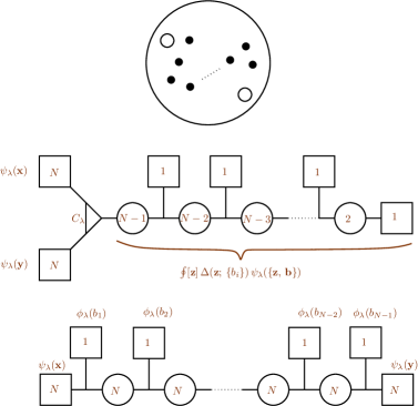
Figure 2: One can determine the structure constants $C_{\lambda}$ of the $A_{n-1}$ theories by studying the theory associated to a sphere with two maximal and $n-1$ minimal punctures (top picture). In one duality frame (middle picture) this is given by a $T_{n}$ theory, involving $C_{\lambda}$, coupled to a “superconformal tail” quiver. In another duality frame (bottom picture) this is given by a linear quiver with an $SU(n)^{n-2}$ gauge group, where each $SU(n)$ is coupled to $2n$ hypermultiplets. For $n=3$, the equivalence of the two frames is the celebrated Argyres-Seiberg duality, whose consequences for the index of $T_{3}$ ($\equiv$ the $E_{6}$ SCFT) have already been explored in section 3.

To include punctures of general type $\Lambda$, we need more general superconformal tails. For each $\Lambda$, there exists a minimal integer $n(\Lambda)$ such that the theory associated to one maximal puncture, one puncture of type $\Lambda$ and $n(\Lambda)$ minimal punctures can be described by a Lagrangian quiver gauge theory Gaiotto:2009we . This can in fact be viewed as a definition of the puncture of type $\Lambda$. By equating the abstract definition of the index of such a theory, namely

$$\sum_{\lambda}\psi_{\lambda}({\bf x})\,\phi_{\lambda}^{\Lambda}({\bf y}_{\Lambda})\,\prod_{i=1}^{n(\Lambda)}\phi_{\lambda}(b_{i})\,,$$ (4.20)

with the explicit integral expression of the same index given by Lagrangian quiver description we can determine the factor $\phi_{\lambda}^{\Lambda}({\bf y}_{\Lambda})$ associated to the puncture of type $\Lambda$.

In summary, we have described an algorithm that determines the superconformal index for all theories of class ${\cal S}$ with regular punctures. The index takes an elegant general form in terms of structure constants $C_{\lambda}(p,q,t)$ and of “wavefunctions” $\{\phi^{\Lambda_{i}}_{\lambda}({\bf y}_{\Lambda_{i}};p,q,t)\}$ associated to the punctures,

$${\cal I}=\sum_{\lambda}C_{\lambda}^{2{g}-2}\,\prod_{j=1}^{s}\phi^{\Lambda_{i}}_{\lambda}({\bf y}_{\Lambda_{i}})\,,$$ (4.21)

where the sum is over the set of finite-dimensional irreps of $\mathfrak{g}=\mathfrak{su}(n)$.

A caveat is in order. Not every possible choice of Riemann surface decorated by a choice of $\{{\Lambda}_{i}\}$ at the punctures corresponds to a physical SCFT. An indication that a choice of decorated surface may be unphysical is if the sum in (4.21) diverges, which happens when the flavor symmetry is “too small”. There are subtle borderline cases where the sum diverges, but the theory is perfectly physical – this can happen when the theory has additional “accidental” flavor symmetries not associated to punctures. An example of such a theory is the rank two $E_{6}$ SCFT. These cases have to be treated with more care Gaiotto:2012uq .

We will discuss how to calculate explicit expressions for the wavefunctions and structure constants in the next section. In the rest of this section we offer two viewpoints that illuminate the structure of the result, the first related to Higgsing and the second to dimensional reduction.

4.4 Higgsing: reduced punctures and surface defects

The index is a meromorphic function of flavor and superconformal fugacities, with a rich structure of poles. A large class of these poles has a nice physical interpretation Gaiotto:2012xa .

Consider a schematic version of the index,

$${\cal I}(a,b)={\rm Tr}(-1)^{F}\,a^{f}\,t^{R}\,,$$ (4.22)

where $f$ and $R$ are two conserved charges. Let us assume that ${\cal I}$ has a pole in fugacity $a$,

$${\cal I}=\frac{\widetilde{\cal I}(a,\,t)}{1-a^{f_{\cal O}}\,t^{R_{\cal O}}}\,.$$ (4.23)

It is natural to associate the pole to a bosonic operator ${\cal O}$, with charges $f=f_{\cal O}$ and $R=R_{\cal O}$, such that an infinite tower of composites of the form ${\cal O}^{n}$ contribute to the index. In the simplest case, ${\cal O}$ is the generator of a ring spanned by $\{{\cal O}^{n}\}$, and the pole appears by resumming the geometric sum,

$$1+a^{f_{\cal O}}\,t^{R_{\cal O}}+(a^{f_{\cal O}}\,t^{R_{\cal O}})^{2}+\dots$$ (4.24)

In more complicated cases, there can be several generators obeying non-trivial relations, which are encoded in the numerator of (4.23). The residue at $a^{f_{\cal O}}\,t^{R_{\cal O}}=1$ is given by $\widetilde{\cal I}(t^{-R_{\cal O}/f_{\cal O}},\,t)$, which can be interpreted as

$${\rm Tr}^{\prime}(-1)^{F}\,\,t^{\bar{R}}\,,\quad\bar{R}\colonequals R-\frac{R_{\cal O}}{f_{\cal O}}\,f\,,$$ (4.25)

where the prime on the trace indicates that we are omitting the infinite set of states with $\bar{R}=0$, which are of course the states responsible for the pole in the first place. The shifted charge $\bar{R}$ is the linear combination of charges preserved in a background where ${\cal O}$ has acquired a non-zero vacuum expectation value (vev). In a path integral representation of the index as the ${\mathbb{S}}^{3}\times{\mathbb{S}}^{1}$ partition function, the divergence at $a^{f_{\cal O}}\,t^{R_{\cal O}}=1$ arises from the integration over a bosonic zero mode, which heuristically we identify with $\langle{\cal O}\rangle$. Following this intuition, we expect the residue to be controlled by the behavior of theory “at infinity” in the moduli space parametrized by $\langle{\cal O}\rangle$, that is, by the properties of the IR theory reached at the endpoint of the the RG flow triggered by giving ${\cal O}$ a vev. We interpret $\widetilde{\cal I}$ as the index of this IR fixed point.

Reducing punctures

As a first application of these ideas, let us obtain more directly the index in the presence of punctures of general type, taking as starting point the index with maximal punctures. The idea is that the theory with a partially-closed puncture can be obtained from the theory with a full puncture by partially higgsing the full $\mathfrak{su}(n)$ flavor symmetry, and flowing to the IR. The role of the operator ${\cal O}$ that featured the above general discussion is played by the moment map operator $\mu$. The moment map is the superconformal primary of the supermultiplet that contains the flavor symmetry current, and thus transforms in the adjoint representation of $\mathfrak{su}(n)$. Given an embedding $\Lambda:\mathfrak{su}(2)\to\mathfrak{su}(n)$, we choose the vev of $\mu$ to be

$$\langle\mu\rangle=\Lambda(t^{-})\in{\rm adj}_{\mathfrak{su}(n)}\,,$$ (4.26)

where $t^{-}$ is the lowest weight of $\mathfrak{su}(2)$. The flavor symmetry is broken down to the centralizer of $\Lambda$ in $\mathfrak{su}(n)$, which we call $\mathfrak{g}_{\Lambda}$. We expect to find poles in the wavefunction $\phi_{\lambda}({\bf a})$ in correspondence to each component of $\mu$ that receives a vev. Extracting the residues with respect to such poles should give the wave function $\phi_{\lambda}^{\Lambda}({\bf x}_{\Lambda})$ associated to the reduced puncture. More precisely, the symmetry breaking also generates Goldstone modes that give a decoupled free sector, and we should remove their contribution if we are interested in the interacting IR SCFT. Finally we should remember to redefine charges, following the general principle outlined in (4.25). In our case, the vev for $\mu$ breaks the $SU(2)_{R}$ symmetry, however a linear combination $\bar{R}$ of the original $R$ Cartan generator and of flavor Cartan generators is preserved; we expect this symmetry to enhance in the IR to the full non-abelian $SU(2)_{\bar{R}}$ of the interacting fixed point. All in all, we have the prescription

$$G^{\Lambda}({\bf a}_{\Lambda})\,\phi^{\Lambda}_{\lambda}({\bf a}_{\Lambda})={\rm Res}_{{\bf a}\to\mathrm{fug}_{{\Lambda}}(\mathbf{a}_{{\Lambda}},t)}\,\phi_{\lambda}({\bf a})\,,$$ (4.27)

where the prefactor $G^{\Lambda}$, which is easily computable, accounts for the contribution to the index of the Goldstone bosons induced by the symmetry breaking. The fugacity replacement ${\bf a}\to\mathrm{fug}_{{\Lambda}}(\mathbf{a}_{{\Lambda}},t)$ can be obtained with a little representation theory. Any representation $\mathfrak{R}$ of $\mathfrak{g}=\mathfrak{su}(n)$ decomposes as

$$\mathfrak{R}=\bigoplus_{j}\mathcal{R}_{j}^{(\mathfrak{R})}\otimes V_{j}\;,$$ (4.28)

where $\mathcal{R}_{j}^{(\mathfrak{R})}$ is some (generally reducible) representation of $\mathfrak{g}_{\Lambda}$ and $V_{j}$ the spin $j$ representation of $\mathfrak{su}(2)$. Then $\mathrm{fug}_{{\Lambda}}(\mathbf{a}_{{\Lambda}},t)$ is the solution for $\mathbf{a}$ in the character decomposition equation,

$$\chi_{\mathfrak{f}}^{\mathfrak{g}}(\mathbf{a})=\sum_{j}\ \chi_{\mathcal{R}_{j}^{(\mathfrak{f})}}^{\mathfrak{g}_{{\Lambda}}}(\mathbf{\mathbf{a}}_{{\Lambda}})\,\chi_{V_{j}}^{\mathfrak{su}(2)}(t^{\frac{1}{2}}\,,t^{-\frac{1}{2}})\;.$$ (4.29)

One can check that (4.27) reproduces the wavefunctions obtained using superconformal tails by the method outlined in the previous subsection. Let us give a couple of simple examples.

Taking $\mathfrak{g}=\mathfrak{su}(2)$ and $\Lambda:\mathfrak{su}(2)\to\mathfrak{su}(2)$ the principal embedding, which in this case is just the identity map, the centralizer is of course trivial and (4.29) reads

$$a+a^{-1}=t^{\frac{1}{2}}+t^{-\frac{1}{2}}\,,$$ (4.30)

which has the two solutions $a=t^{\frac{1}{2}}\,,t^{-\frac{1}{2}}\,$, related by the action of the Weyl group $a\leftrightarrow a^{-1}$. Since we are interested in the vev of the $\mathfrak{su}(2)$ lowest weight $\mu^{-}$ of the moment map, whose contribution to the index is $a^{-2}t$, we should pick $a=t^{\frac{1}{2}}$; the other solution $t^{-\frac{1}{2}}$ would be associated to the $\mathfrak{su}(2)$ highest weight $\mu^{+}$. The lesson (which generalizes) is that if we are interested in giving a vev to specific operator, we should fix a representative of the Weyl orbit. Extracting the residue at $a^{2}t^{-1}=1$ will give the index of the IR theory at the end of the RG flow triggered by $\langle\mu^{-}\rangle$, times the contribution from the free Goldstone bosons. In this case, the Goldstone bosons consist of a free hypermultiplet in the fundamental of the flavor $\mathfrak{su}(2)$. Both the flavor and $R$ symmetry are broken by the vev, but the combination $\bar{R}=R+f/2$ is preserved. Under the new $SU(2)_{\bar{R}}$, the scalars of the free hypermultiplet transform as ${\bf 3}+{\bf 1}$, with the singlet corresponding to the states responsible for the divergence. Extracting the pole is precisely equivalent to omitting this singlet states. Setting $a=t^{\frac{1}{2}}$ in (2.9) we see that under this new charge assignment the non-singlet states of the free hypermultiplet give a contribution to the index exactly equal to the inverse of the index of a free $U(1)$ vector multiplet, so the Goldstone boson factor in (4.27) is $G={\cal I}_{V}^{-1}$. All in all, we have derived from general principles the following prescription to close an $\mathfrak{su}(2)$ puncture,

$${\cal I}_{V}\,{\rm Res}_{a^{-2}t\to 1}\,\phi^{[1^{2}]}_{\lambda}(a)=\phi_{\lambda}^{[2]}\equiv 1\,.$$ (4.31)

In the last equality we have just reminded ourselves that the wavefunction of a fully closed puncture is identically equal to one. One can check (4.31) using the expression for $\phi^{[1^{2}]}_{\lambda}$ derived by the methods of the previous subsection.

A sightly more involved example is $\mathfrak{g}=\mathfrak{su}(3)$ and $\Lambda$ the subregular embedding, corresponding to the partition $[2,1]$. The centralizer is $\mathfrak{g}_{\Lambda}=\mathfrak{u}(1)$. If $a_{1}$, $a_{2}$, $a_{3}$ with $a_{1}a_{2}a_{3}=1$ are the $\mathfrak{su}(3)$ fugacities, and $b$ the $\mathfrak{u}(1)$ fugacity, (4.29) takes the form

$$a_{1}+a_{2}+a_{3}=b\,(t^{\frac{1}{2}}+t^{-\frac{1}{2}})+b^{-2}\,.$$ (4.32)

The only solution (up to the action of the Weyl group, which permutes the $a_{i}$) is $a_{1}=t^{\frac{1}{2}}b$, $a_{2}=t^{-\frac{1}{2}}b$, $a_{3}=b^{-2}$. Extracting the residue and removing the contribution of the Goldstone bosons accomplishes the reduction of the full puncture to the minimal puncture.

Surface defects

Next, we would like to interpret in a similar light the poles (4.12) that played such a crucial role in the previous subsection. Recall the basic setup: we “glued” the bifundamental hypermultiplet theory $T_{n}^{[1^{n}]\,[1^{n}]\,[n-1,1]}$ to a general theory $T[{\cal C}]$, connecting a maximal puncture of one theory with a maximal puncture of the other theory by gauging the diagonal $SU(n)$ symmetry. We then extracted residues with respect to the fugacity $a$ for the $U(1)$ global symmetry of the hypermultiplet. This is the $U(1)$ baryon symmetry, under which the complex scalars $q$ and $\tilde{q}$ have charge $-1$ and $+1$ respectively. It is then clear that the operator associated to the simplest pole, at $a^{-n}t^{\frac{n}{2}}=1$, is the baryon operator $B={\rm det}\;q$. Giving a vev to $B$ higgses the $SU(n)$ gauge group, triggering an RG flow whose IR endpoint is the original theory $T[{\cal C}]$ and a collection of decoupled free fields Gaiotto:2012xa . This explains (4.13).

By the same logic, the poles at $p^{r}q^{s}t^{\frac{n}{2}}a^{-n}=1$ are naturally associated to holomorphic derivatives of the baryon operator in the $12$ and $34$ planes, $\partial^{r}_{12}\,\partial^{s}_{34}\,\det q$. We expect the residue at these poles to describe the IR physics of the flow triggered by a spacetime-dependent vev of the form $\langle B\rangle\sim z^{r}w^{s}$. Consider first the $r=0$, $s\neq 0$ case. Away from the $w=0$ plane, the endpoint of the flow is still $T[{\cal C}]$. However some extra degrees of freedom survive at $w=0$, which we interpret as a surface defect for $T[{\cal C}]$ extended in the 12 plane. Similarly, the endpoint of the flow with $r\neq 0$, $s=0$ is $T[{\cal C}]$ decorated with an extra surface defect extended in the 34 plane. In the general case with $rs\neq 0$ both type of defects will be present. In the ${\mathbb{S}}^{3}\times{\mathbb{S}}^{1}$ geometry, these surface defects fill the “temporal” ${\mathbb{S}}^{1}$ and the two maximal circles inside the ${\mathbb{S}}^{3}$ fixed by the $j_{12}$ and $j_{34}$ rotations, respectively. This proposal has been checked Gadde:2013dda in a set of examples where $T[{\cal C}]$ admits a Lagrangian description, and surface defects can be added by coupling the $4d$ SCFT to a $(2,2)$ sigma model; the index can then be independently evaluated by localization techniques, confirming the prescription that we have just outlined.

In summary, we have found a physical interpretation for the difference operators ${\mathfrak{S}}_{(r,s)}$: their action on the index of $T[{\cal C}]$ yields the index of the same theory decorated by some extra surface defect Gaiotto:2012xa . Since the difference operators act “locally” on the generalized quiver, we should associate them to special punctures of the UV curve. This agrees with the M-theory picture, where the surface defects correspond to M2 branes localized on the UV curve. Acting with a difference operator on a given flavor fugacity corresponds pictorially to colliding the special puncture with a flavor puncture. The location of the special punctures on the UV curve is immaterial, so collision of the same special puncture with different flavor punctures is bound to give the same result – which is a restatement of (4.15).

This description of surface defects bears a striking kinship with the analogous picture that arises in the AGT correspondence  Alday:2009aq ; Alday:2009fs . The introduction of surface defects in the ${\mathbb{S}}^{4}$ partition function is accomplished by the insertion of special, semi-degenerate operators in the Toda CFT correlator defined on the UV curve. These operators are the key to the solution of Liouville theory by the conformal bootstrap Teschner:1995yf : considering their fusion with normalizable vertex operators one can derive functional equations that admit a unique solution. Similarly, we have special punctures in our 2d TQFT that insert surface defects in the ${\mathbb{S}}^{3}\times{\mathbb{S}}^{1}$ partition function. Their fusion with ordinary flavor punctures leads to the topological bootstrap equations (4.31), which uniquely fix the superconformal index.

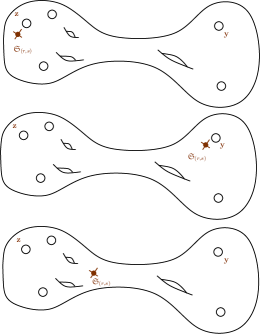
Figure 3: The difference operators ${\mathfrak{S}}_{(r,s)}$, which compute residues and introduce surface defects, can be visualized as special punctures on the UV curve. The action of ${\mathfrak{S}}_{(r,s)}$ on a flavor fugacity is interpreted as the collision of the special puncture with a flavor puncture. We can act on different punctures and obtain the same result for the index (top and middle pictures). We can also define the action of ${\mathfrak{S}}_{(r,s)}$ on a long tube (bottom picture), by cutting open a cylinder, acting on one of the open punctures and gluing the surface back. S-duality guarantees that this is a well-defined procedure. In this way we can introduce the special punctures ${\mathfrak{S}}_{(r,s)}$ on a UV curve with no flavor punctures at all.

4.5 Reduction to 3d

The index of theories of class ${\cal S}$ has a very definite structure (4.21). This structure is natural since it is a manifestation of the $2d$ TQFT nature of the index of the theories at hand as was anticipated in section 4.2. It is however an important question to understand better the physical meaning of the different ingredients entering (4.21). For example, we would like to gain more insight into the physical significance of the eigenfunctions $\phi^{\Lambda_{i}}_{\lambda}({\bf y}_{\Lambda_{i}})$ and the eigenvalues ${\cal E}_{\lambda}^{(r,s)}$. Let us consider here a very informative $3d$ interpretation of (4.21).

We can consider theories of class ${\cal S}$ on ${\cal M}_{3}\times{\mathbb{S}}^{1}$ with ${\cal M}_{3}$ some three dimensional manifold. Upon reduction on the ${\mathbb{S}}^{1}$ we obtain a $3d$ theory on ${\cal M}_{3}$. The ${\cal N}=2$ class ${\cal S}$ theories admitting a known description in terms of a Lagrangian upon dimensional reduction on ${\mathbb{S}}^{1}$ are described in terms of the same field content and same gauge and superpotential interaction as the $4d$ parent theory. The $3d$ Lagrangians however are not conformal and the theories flow in general to an interacting ${\cal N}=4$ $3d$ SCFT in the IR. The $4d$ conformal S-dualities imply IR (Seiberg-like) dualities of the $3d$ models. Thus the complex moduli of the Riemann surface defining the model in $4d$ do not translate to physical parameters in $3d$: the topology of the surface and the information at the punctures alone are sufficient to completely specify the $3d$ model. An extremely interesting fact about the class ${\cal S}$ theories in $3d$ is that they possess yet another dual description. All theories of class ${\cal S}$ reduced to $3d$, with and without known Lagrangian description in $4d$, have a mirror description in $3d$ in terms of a star-shaped quiver theory Benini:2010uu .

This mirror symmetry states that a theory corresponding to a Riemann surface with genus $g$ and $s$ punctures of types $\Lambda_{i}$ is dual to a quiver theory coupling $s$ linear quivers ${\mathfrak{T}}_{\Lambda_{i}}[{\mathfrak{g}}]$ Gaiotto:2008ak associated to Lie algebra ${\mathfrak{g}}=\mathfrak{su}(N)$ by gauging the common ${\mathfrak{g}}$ with an addition of $g$ ${\cal N}=4$ adjoint hypermultiplet, see figure 4 for an example.

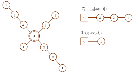
Figure 4: On the left we have an example of a star-shaped quiver mirror of the $A_{3}$ theory corresponding to a sphere with four punctures, two of which are maximal and one is minimal. On the right the quiver theories for ${\mathfrak{T}}_{(1,1,1,1)}[\mathfrak{su}(4)]$ corresponding to the maximal puncture and ${\mathfrak{T}}_{(3,1)}[\mathfrak{su}(4)]$ corresponding to minimal puncture are depicted.

The dimensional reduction on ${\mathbb{S}}^{1}$ can be performed at the level of the index. Here ${\cal M}_{3}$ is ${\mathbb{S}}^{3}$ and upon reduction of the index on ${\mathbb{S}}^{1}$ we obtain the partition function of the dimensionally reduced theory on a squashed sphere ${\mathbb{S}}^{3}_{b}$ Dolan:2011rp ; Gadde:2011ia ; Imamura:2011uw (see also Aharony:2013dha ). The reduction is done by first parametrizing the fugacities as

$$t=e^{2\pi ir_{1}(\gamma+\frac{i}{2r_{3}}(b+b^{-1}))},\;\;\;z=e^{2\pi ir_{1}\sigma},\;\;\;p=e^{2\pi br_{1}/r_{3}},\;\;\;q=e^{2\pi b^{-1}r_{1}/r_{3}}\,,$$ (4.33)

where $r_{1}$ is the radius of ${\mathbb{S}}^{1}$ and $r_{3}$ is the radius of ${\mathbb{S}}^{3}$. Then the radius of ${\mathbb{S}}^{1}$, $r_{1}$, is sent to zero. The parameter $b$ is the squashing parameter of the sphere.

We have defined the functions $\phi^{\Lambda_{i}}_{\lambda}({\bf y}_{\Lambda_{i}})$ as eigenfunctions of difference operators ${\mathfrak{S}}_{(r,s)}$ and argued that this operators have a physical interpretation of introducing linked surface defects to the index computation. The surface defects corresponding to ${\mathfrak{S}}_{(0,s)}$ and ${\mathfrak{S}}_{(r,0)}$ span the ${\mathbb{S}}^{1}$ and one of the two equators of ${\mathbb{S}}^{3}$. Upon reduction on the ${\mathbb{S}}^{1}$ these become line defects sitting on one of the two equators of ${\mathbb{S}}^{3}_{b}$. When sending $r_{1}\to 0$ the difference operators have very simple limit. For example in the $A_{1}$ case we have

$${\mathfrak{S}}_{(0,1)}\cdot f(z)\qquad\to\qquad{\cal T}(\sigma)\cdot\hat{f}(\sigma)=$$

$$\,\qquad=\frac{\sinh\pi b\left(\frac{i(b-b^{-1})}{2}-\gamma+2\sigma\right)}{\sinh 2\pi b\sigma}\hat{f}(\sigma+\frac{ib}{2})+\frac{\sinh\pi b\left(\frac{i(b-b^{-1})}{2}-\gamma-2\sigma\right)}{\sinh-2\pi b\sigma}\hat{f}(\sigma-\frac{ib}{2})\,,$$

where $\hat{f}(\sigma)=\lim_{r_{1}\to 0}f(e^{2\pi ir_{1}\sigma})$. Interestingly a set of eigenfunctions of this operator is given by the ${\mathbb{S}}^{3}_{b}$ partition functions of the ${\mathfrak{T}}[\mathfrak{su}(2)]$ theory. The ${\mathfrak{T}}[\mathfrak{su}(N)]$ theory has global $\mathfrak{su}(N)_{H}\times\mathfrak{su}(N)_{C}$ symmetry with the $\mathfrak{su}(N)_{H}$ acting on the Higgs branch and $\mathfrak{su}(N)_{C}$ acting on the Coulomb branch. Turning on real mass parameters, ${\bf\sigma}_{H}$ and ${\bf\sigma}_{C}$, for the two symmetries the ${\mathbb{S}}^{3}_{b}$ partition function of ${\mathfrak{T}}[\mathfrak{su}(N)]$ can be denoted by $\phi^{({\gamma,b})}({\bf\sigma}_{H}|{\bf\sigma}_{C})$ and we have the property

$${\cal T}({\bf\sigma}_{C})\cdot\phi^{({\gamma,b})}({\bf\sigma}_{H}|{\bf\sigma}_{C})={\cal W}({\bf\sigma}_{H})\,\phi^{({\gamma,b})}({\bf\sigma}_{H}|{\bf\sigma}_{C})\,.$$ (4.35)

The eigenvalue ${\cal W}({\bf\sigma}_{H})$ is the expectation value of the Wilson loop for the $\mathfrak{su}(N)_{H}$ global symmetry. This eigenvalue property of the partition function thus suggests the physical interpretation that the line defect for the gauge symmetry of ${\mathfrak{T}}[\mathfrak{su}(N)]$ is equivalent to a Wilson line for the global $\mathfrak{su}(N)_{H}$ symmetry. This fact is not surprising since the ${\mathfrak{T}}[\mathfrak{su}(N)]$ theories make their appearance as models living on S-duality domain wall separating two S-dual ${\cal N}=4$ $SU(N)$ SYM theories. Since under $4d$ S-duality defect (’t Hooft) line operators map to Wilson operators our $3d$ eigenvalue statement is natural.

Further, the ${\mathbb{S}}^{3}_{b}$ partition function of a star shaped quiver mirror dual say to the $A_{1}$ theory with genus $g$ and $s$ punctures has the following form,

$$Z_{g,s}(\{\sigma^{(i)}_{C}\}_{i=1}^{s})=\int d\sigma_{H}Z_{V}(\sigma_{H})\;Z_{\cal H}(\sigma_{H})^{g}\;\prod_{i=1}^{s}\phi^{(\gamma,b)}(\sigma_{H}|\sigma^{(i)}_{C})\,.$$ (4.36)

Here $Z_{\cal H}(\sigma_{H})$ is the contribution of an ${\cal N}=4$ $3d$ adjoint hypermultiplet and $Z_{V}(\sigma_{H})$ is the contribution of the vector. Note the striking structural similarity between (4.21) and (4.36). This is not a coincidence Nishioka:2011dq . One can argue that indeed in the $r_{1}\to 0$ limit the eigenfunctions $\phi^{\Lambda}_{\lambda}({\bf y}_{\Lambda})$ reduce to the ${\mathbb{S}}^{3}_{b}$ partition functions of ${\mathfrak{T}}_{\Lambda}[\mathfrak{su}(N)]$. The discrete labels of the eigenfunctions, $\lambda_{i}$, become (linear combinations of) the real masses of the symmetry rotating the Coulomb branch of ${\mathfrak{T}}_{\Lambda}[\mathfrak{su}(N)]$, $\sigma^{(i)}_{C}$: roughly, taking the $r_{1}\to 0$ limit we should also concentrate on large representations and keep $r_{1}\,\lambda_{i}$ fixed.

Let us summarize the $3d$ interpretation of the eigenfunctions,

• The difference operators introduce line defects.

• The eigenfunctions are ${\mathbb{S}}^{3}_{b}$ partition functions of ${\mathfrak{T}}_{\Lambda}[\mathfrak{su}(N)]$.

• The eigenvalues are expectation values of Wilson loops.

• The existence of the eigenvalue equation follows from $4d$ S-duality through the statement that Wilson and ’t Hooft lines are S-dual to each other.

In particular the fact that the index of theories of class ${\cal S}$ in $4d$ can be written in the form (4.21) is a $4d$ manifestation of the fact that the dimensionally reduced theories admit a mirror description. That is the index written as (4.21) is a $4d$ precursor of the $3d$ mirror symmetry. The interested reader might consult Razamat:2014pta for more thorough discussion of these issues.

Finally let us also mention that the $3d$ eigenfunctions, ${\mathbb{S}}^{3}_{b}$ partition functions of ${\mathfrak{T}}_{\Lambda}[\mathfrak{su}(N)]$, provide a connection between the $4d$ index and the $4d$ ${\mathbb{S}}^{4}$ partition functions of theories of class ${\cal S}$. As we mentioned ${\mathfrak{T}}_{\Lambda}[\mathfrak{su}(N)]$ models are obtained by considering ${\cal N}=4$ $4d$ theories with a duality domain wall. The kernel which implements the insertion of such duality wall in the ${\mathbb{S}}^{4}$ partition function computation is precisely the ${\mathbb{S}}^{3}_{b}$ partition function of ${\mathfrak{T}}_{\Lambda}[\mathfrak{su}(N)]$ Hosomichi:2010vh . In particular the difference operator we obtained by reduction to $3d$ are the same difference operators introducing line defects into Liouville-Toda/${\mathbb{S}}^{4}$ (AGT correspondence Alday:2009aq ) computations Gaiotto:2012xa (see also Bullimore:2014nla ).

5 Integrable models and limits of the index

The discussion of the previous section reduces the physical problem of determining the superconformal index of class ${\cal S}$ theories to the mathematical problem of finding a complete set of orthonormal eigenfunctions of the difference operators ${\mathfrak{S}}_{(r,s)}({\bf x})$. Remarkably, these operators are closely related to the Hamiltonians that define a well-known class of integrable models, the elliptic relativistic Ruijsenaars-Schneider (RS) models, aka relativistic elliptic Calogero-Moser-Sutherland models.

The operator (4.14), ${\mathfrak{S}}_{(0,1)}({\bf x})$, is related to the basic RS Hamiltonian ${\cal H}_{1}(t,q;p)$ by a similarity transformation,

$${\cal H}_{1}(t,q;p)=\frac{\theta(q^{-1};p)}{\theta(t;p)}\;\frac{1}{\prod_{i\neq j}\Gamma(t\,z_{i}/z_{j};p,\,q)}\;{\mathfrak{S}}_{(0,1)}({\mathbf{z}})\;\prod_{i\neq j}\Gamma(t\,z_{i}/z_{j};p,\,q)\,.$$ (5.1)

Under the same similarity transformation, the propagator measure in the $A_{n-1}$ case becomes

$$\frac{1}{n!}\oint\prod_{i=1}^{n-1}\frac{dz_{i}}{2\pi iz_{i}}\prod_{i\neq j}\frac{\Gamma(t\,z_{i}/z_{j};p,\,q)}{\Gamma(z_{i}/z_{j};p,\,q)}\,\cdots\,.$$ (5.2)

Higher operators, ${\cal H}_{\ell}$, can be constructed as polynomials in ${\mathfrak{S}}_{(0,s)}$. One can think of the $n-1$ independent ${\cal H}_{\ell}$ operators as associated to antisymmetric representations of $SU(n)$, whereas ${\mathfrak{S}}_{(0,s)}$ are associated to symmetric representations. Then by exploiting group theory and the fact that the fundamental representation can be trivially thought as either symmetric or antisymmetric one can translate between ${\cal H}_{\ell}$ and ${\mathfrak{S}}_{(0,s)}$ (see for example Bullimore:2014nla ).

The parameters $p$, $q$, and $t$ appear in the Hamiltonian ${\cal H}_{1}(t,q;p)$ on different footing: (i) the parameter $t$ plays a role of coupling constant, (ii) $q$ is the shift parameter of the difference operator and can be understood as an exponent of the “speed of light” parameter of the relativistic integrable system, (iii) the integrable model is associated to an elliptic curve parametrized by $p$. Given an eigenfunction of ${\cal H}_{1}$ dressing it with an arbitrary elliptic function in $q$ a huge class of new eigenfunctions can be obtained. This arbitrariness is lifted by the demand that the eigenfunction we are after diagonalize both operators ${\mathfrak{S}}_{(0,s)}$ and ${\mathfrak{S}}_{(s,0)}$ and in particular are symmetric with respect to exchanging $p$ and $q$.

The RS models have a long history of rich connections with gauge theories in various dimensions (see e.g. gorsky ; Gorsky:1993pe ). Nevertheless, for general values of $(p,q,t)$ determining the exact eigenfunctions and eigenvalues of the difference operators is still an open problem. For some natural limits of the parameters the eigenfunctions are well known. Curiously, many of the same limits have independent physical interest, because they lead to a supersymmetry enhancement of the ${\mathbb{S}}^{3}\times{\mathbb{S}}^{1}$ partition function. One can systematically classify the limits of the index that enjoy enhanced supersymmetry, and relate them to integrable models. We will shortly review some of the salient results in this direction. Physical properties of theories of class ${\cal S}$ impose additional constraints on $\phi_{\lambda}({\bf z})$. For example, since some of the theories have known Lagrangian descriprion the indices can be explicitly computed as integrals of elliptic Gamma functions and the results have to match the expressions evaluated using the eigenfunctions. Exploiting the known expressions for the eigenfunctions for specialized values of the parameters and the additional physical constraints one can set up a perturbative scheme around the known results to compute the eigenfunctions for general values of the parameters Gaiotto:2012xa ; Razamat:2013qfa .

We now turn to discuss several useful limits of the index for which explicit expressions for eigenfunctions are known.

Schur index

The trace formula (2.2) that defines the general index can be written in the following equivalent form (we suppress flavor fugacities to avoid cluttering):

$${\cal I}(q,p,t)=\mathrm{Tr}(-1)^{F}\,p^{\frac{1}{2}\delta^{1}_{-}}\,q^{\frac{1}{2}\delta^{1}_{+}}\,t^{R+r}\,e^{-\beta^{\prime}\delta_{2\dot{-}}}\,,$$ (5.3)

where

$$2\delta^{1}_{+} \colonequals\{{\cal Q}^{1}_{+}\,,({\cal Q}^{1}_{+})^{\dagger}\}= E+2j_{1}-2R-r\geqslant 0$$ (5.4)

$$2\delta^{1}_{-} \colonequals\{{\cal Q}^{1}_{-}\,,({\cal Q}^{1}_{-})^{\dagger}\}= E-2j_{1}-2R-r\geqslant 0$$

$$2\delta_{2\dot{-}} \colonequals\{{\widetilde{\cal Q}}_{2\dot{-}}\,,({\widetilde{\cal Q}}_{2\dot{-}})^{\dagger}\}= E-2j_{2}-2R+r\geqslant 0\,.$$

The inequalities follow from unitarity of the representation and will be useful momentarily. The equivalence of (2.2) and (5.3) follows immediately by recalling that only states with $\delta_{2\dot{-}}=0$ contribute to the trace. The Schur index is the “unrefined” index obtained by setting $q=t$.  . One readily observes that on this slice the combination of conserved charges appearing in the trace formula commute with a second supercharge, ${\cal Q}^{1}_{-}$, in addition to the supercharge $\widetilde{\cal Q}_{2\dot{-}}$ that leaves invariant the general index. As the $p$ dependence is ${\cal Q}^{1}_{-}$-exact, it drops out, and we are left with a simple expression that depends on $q$ alone,

$${\cal I}_{\rm Schur}\colonequals\mathrm{Tr}(-1)^{F}\,q^{E-R}\,.$$ (5.5)

The index counts operators with $\delta^{1}_{-}=\delta_{2\dot{-}}=0$, or equivalently

$$\widehat{L}_{0}\colonequals\frac{E-(j_{1}+j_{2})}{2}-R=0\,,\qquad{\cal Z}\colonequals j_{1}-j_{2}+r=0\,.$$ (5.6)

In fact, the unitarity inequalities in (5.4) give $\widehat{L}_{0}\geqslant\frac{|{\cal Z}|}{2}$, so the first condition implies the second. We refer to operators obeying $\widehat{L}_{0}=0$ as Schur operators. A Schur operator is annihilated by two Poincaré supercharges of opposite chiralities (${\cal Q}_{-}^{1}$ and $\widetilde{\cal Q}_{2\dot{-}}$ in our conventions). This is a consistent condition because the supercharges have the same $SU(2)_{R}$ weight, and thus anticommute with each other. No analogous BPS condition exists in an $\mathcal{N}=1$ supersymmetric theory, because the anticommutator of opposite-chirality supercharges necessarily yields a momentum operator, which annihilates only the identity.

Multiplet	$\mathcal{O}_{\rm Schur}$	$h\colonequals\frac{E+(j_{1}+j_{2})}{2}$	$r$	Lagrangian “letters”
$\hat{\mathcal{B}}_{R}$	$\Psi^{11\dots 1}$	$R$	$0$	$Q$, $\tilde{Q}$
$\mathcal{D}_{R(0,j_{2})}$	$\widetilde{\mathcal{Q}}^{1}_{\dot{+}}\Psi^{11\dots 1}_{\dot{+}\dots\dot{+}}$	$R+j_{2}+1$	$j_{2}+\frac{1}{2}$	$Q$, $\tilde{Q}$, $\tilde{\lambda}^{1}_{\dot{+}}$
$\bar{\mathcal{D}}_{R(j_{1},0)}$	${\mathcal{Q}}^{1}_{+}\Psi^{11\dots 1}_{+\dots+}$	$R+j_{1}+1$	$-j_{1}-\frac{1}{2}$	$Q$, $\tilde{Q}$, $\lambda^{1}_{+}$
$\hat{\mathcal{C}}_{R(j_{1},j_{2})}$	${\mathcal{Q}}^{1}_{+}\widetilde{\mathcal{Q}}^{1}_{\dot{+}}\Psi^{11\dots 1}_{+\dots+\,\dot{+}\dots\dot{+}}$	$R+j_{1}+j_{2}+2$	$j_{2}-j_{1}$	$D_{+\dot{+}}^{n}Q$, $D_{+\dot{+}}^{n}\tilde{Q}$, $D_{+\dot{+}}^{n}\lambda^{1}_{+}$, $D_{+\dot{+}}^{n}\tilde{\lambda}^{1}_{\dot{+}}$

Table 3: This table summarizes the manner in which Schur operators fit into short multiplets of the $\mathcal{N}=2$ superconformal algebra. We use the naming conventions for supermultiplets of Dolan and Osborn Dolan:2002zh . For each supermultiplet, we denote by $\Psi$ the superconformal primary. There is then a single conformal primary Schur operator ${\mathcal{O}}_{\rm Schur}$, which in general is obtained by the action of some Poincaré supercharges on $\Psi$. We list the holomorphic dimension $h$ and $U(1)_{r}$ charge $r$ of ${\mathcal{O}}_{\rm Schur}$ in terms of the quantum numbers $(R,j_{1},j_{2})$ that label the shortened multiplet (left-most column). We also indicate the schematic form that ${\mathcal{O}}_{\rm Schur}$ can take in a Lagrangian theory by enumerating the elementary “letters” from which the operator may be built. We denote by $Q$ and $\tilde{Q}$ the complex scalar fields of a hypermultiplet, by $\lambda_{\alpha}^{\mathcal{I}}$ and $\tilde{\lambda}_{\dot{\alpha}}^{\mathcal{I}}$ the left- and right-moving fermions of a vector multiplet, and by $D_{\alpha\dot{\alpha}}$ the gauge-covariant derivatives. Note that while in a Lagrangian theory Schur operators are built from these letters, the converse is false – not all gauge-invariant words of this kind are Schur operators, only the special combinations with vanishing anomalous dimensions.

A summary of the different classes of Schur operators, organized according to how they fit in shortened multiplets of the superconformal algebra, is given in Table 3 Beem:2013sza . The first line lists the half-BPS operators belonging to the Higgs branch ${\cal N}=1$ chiral ring, which have $E=2R$ and $j_{1}=j_{2}=0$. In a Lagrangian theory, these are operators of the schematic form $QQ\dots\tilde{Q}\tilde{Q}$. The $SU(2)_{R}$ highest weight component of the moment map operator $\mu^{11}$, which has $E=2R=2$ (and transforms in the adjoint representation of the flavor group) is in this class. The second and third lines of the table list more general ${\cal N}=1$ antichiral (respectively chiral) operators. In a Lagrangian theory they may be obtained by considering gauge-invariant words that contain $\tilde{\lambda}^{1}_{\dot{+}}$ (respectively $\lambda^{1}_{+}$) in addition to $Q$ and $\tilde{Q}$. Finally the forth line lists the most general class of Schur operators, belonging to supermultiplet obeying less familiar semishortening conditions. An important operator in this class is the Noether current for the $SU(2)_{R}$ R-symmetry, which belongs to the same superconformal multiplet as the stress-energy tensor and is universally present in any ${\cal N}=2$ SCF. Its $J^{11}_{+\dot{+}}$ component, with $E=3$, $R=1$, $j_{1}=j_{2}=\frac{1}{2}$, is a Schur operator. Finally, note that the half-BPS operators of the Coulomb branch chiral ring (of the form ${\rm Tr}\,\phi^{k}$ in a Lagrangian theory) are not Schur operators.

The Schur index earns its name from the fact that the wavefunctions are proportional to Schur polynomials, and simple closed form expressions are available for all the ingredients that enter the TQFT formula for the index (4.21). We will quote the full expressions below in the more general Macdonald limit. The structure constants $C_{\lambda}(q)$ turn out to be inversely proportional to the quantum dimension of the representation $\lambda$. One recognizes Gadde:2011ik the TQFT of the index as the zero-area limit of $q$-deformed $2d$ Yang-Mills theory Aganagic:2004js , which can also be understood as an analytic continuation of Chern-Simons theory on ${\cal C}\times{\mathbb{S}}^{1}$. This observation has been reproduced by a top-down approach  Kawano:2012up ; Fukuda:2012jr , starting from the $(2,0)$ theory on the geometry ${\mathbb{S}}^{3}\times{\mathbb{S}}^{1}\times{\cal C}$, first reducing on ${\mathbb{S}}^{1}$ to obtain $5d$ YM, and then reducing further on ${\mathbb{S}}^{3}$ and using supersymmetric localization to obtain a bosonic gauge theory on ${\cal C}$, which is argued to coincide with $q$-YM.

In $q$-YM theory, introducing flavor punctures correspond to fixing the holonomies of the gauge fields around the punctures. One can also define additional local operators by fixing the dual variables at the punctures Witten:1991we – in the language of Chern-Simons theory on ${\cal C}\times{\mathbb{S}}^{1}$, this corresponds to adding a Wilson loop along the temporal ${\mathbb{S}}^{1}$. These operators are the natural candidates to correspond to the surface defects discussed in the previous section Gaiotto:2012xa ; Alday:2013kda .

Perhaps the most interesting fact about the Schur index is that it can be viewed as the character of a $2d$ chiral algebra canonically associated to the $4d$ SCFT Beem:2013sza , as we shall review in section 7. A related point is that the Schur index enjoys intriguing modular properties encoding conformal anomalies Razamat:2012uv . For example the indices of a hypermultiplet and the vecor multiplets in the Schur limit become combinations of theta functions,

$${\cal I}_{H}=\frac{1}{\theta(q^{\frac{1}{2}}a;q)}\,,\qquad\Delta_{Haar}({\bf z})\,{\cal I}_{V}({\bf z})=\frac{1}{n!}(q;q)^{2n-2}\prod_{i\neq j}\theta(qz_{i}/z_{j};q)\,,$$ (5.7)

which have simple modular properties under

$$q=e^{2\pi i\tau}\quad\to\quad q^{\prime}=e^{-\frac{2\pi i}{\tau}},\qquad z=e^{2\pi i\zeta}\quad\to\quad z^{\prime}=e^{\frac{2\pi i\zeta}{\tau}}\,.$$ (5.8)

Here $\Delta_{Haar}$ is the Haar measure and we specialized for concreteness to $SU(n)$ vector field. An index of the gauge theory is given by contour integrals with the integrand built from products of theta functions. The combination of theta functions in in the integrand, ${\cal I}_{integ.}({\bf z};q)$, always forms an elliptic function in the fugacities, ${\bf z}$ corresponding to the gauged symmetries,

$${\cal I}_{integ.}(q\,{\bf z};q)={\cal I}_{integ.}({\bf z};q)\,.$$ (5.9)

The gauge fugacities ${\bf z}$ can be thus thought as taking values on a torus with modular parameter $\tau$. The contour integral defining the Schur index of a gauge theory then can be thought of as an integral over a cycle of the torus while the index after modular transformation is given as an integral over the dual cycle.

Figure 5: The Schur index of a guage theory is given by an integral over fugacities ${\bf z}$ taking value in a torus with modular parameter $\tau$. After modular transformation, $\tau\to-\frac{1}{\tau}$, the index is written as an integral over the dual cycle.

These properties beg the question of the relation of the Schur index to mock modular forms, a relation which is yet to be explored.

Macdonald limit

Taking $p\to 0$ in (5.3) is a well-defined limit, thanks to positive-definiteness of the associated charge $\delta^{1}_{-}$. The trace formula reads

$${\cal I}_{\rm Mac}(q,t)\colonequals{\rm Tr}_{\rm M}(-1)^{F}q^{E-2R-r}t^{R+r}={\rm Tr}_{\rm M}(-1)^{F}q^{2j_{1}}t^{R+r}\,,$$ (5.10)

where the subscript in the trace indicates that we are restricting by hand to the states with $\delta^{1}_{-}=0$. Clearly, we are concentrating on the operators that are also annihilated by the supercharge ${\cal Q}^{1}_{-}$, in addition to $\widetilde{\cal Q}_{2\dot{-}}$. These are of course the same as the Schur operators, but we are now refining their counting by keeping track of the quantum number $R+r$. For $q=t$, we recover the Schur index.

This limit is mathematically very interesting. Our difference operators and our integration measure become identical (up to conjugation) to the well-studied Macdonald difference operators and Macdonald measure Mac . The diagonalization problem is completely solved in terms of Macdonald polynomials, a beautiful two-parameter generalization of the Schur polynomials. In the Macdonald limit we set the elliptic curve of the Ruijsenaars-Schneider model, $p$, to zero the integrable model becomes thus trigonometric (but still relativistic). For example, in the $A_{1}$ case after conjugation (5.1) the basic hamiltonian becomes,

$${\cal H}_{1}\cdot f(z)\sim\frac{1-t\,z^{2}}{1-z^{2}}\,f(q^{\frac{1}{2}}z)+\frac{1-t\,z^{-2}}{1-z^{-2}}\,f(q^{-\frac{1}{2}}\,z)\,.$$ (5.11)

We are then able to find closed form expressions for the general wavefunctions and for the structure constants Gadde:2011uv . The wavefunction for a general choice of puncture (embedding) and representation now takes the following form,

$$\psi_{\mathfrak{R}}^{\Lambda}({\bf z}_{\Lambda};q,t)=K_{\Lambda}({\bf z}_{\Lambda};q,t)\,P_{\mathfrak{R}}^{\mathfrak{g}}(\mathrm{fug}_{\Lambda}(\mathbf{z}_{\Lambda};t);q,t)~{}.$$ (5.12)

Here $P_{\mathfrak{R}}^{\mathfrak{g}}(\mathbf{z};q,t)$ are the Macdonald polynomials labeled by finite dimensional representatioins $\mathfrak{R}$ of Lie algebra $\mathfrak{g}$ and orthonormal under the Macdonald measure, which, e.g., for $\mathfrak{g}={\mathfrak{su}}(n)$ is given by,

$$\Delta_{q,t}({\bf z})=\frac{1}{n!}\prod_{i\neq j}\frac{(z_{i}/z_{j};q)}{(tz_{i}/z_{j};q)}\,.$$ (5.13)

The $K$-factors admit a compact expression as a plethystic exponential Mekareeya:2012tn ,

$$K_{\Lambda}(\mathbf{z}_{\Lambda};q,t)=\mathrm{P.E.}\left[\sum_{j}\frac{t^{j+1}}{1-q}\raisebox{1.0pt}{$\chi$}^{\mathfrak{h}_{\Lambda}}_{\mathcal{R}_{j}^{(\mathrm{adj})}}(\mathbf{z}_{\Lambda})\right]~{},$$ (5.14)

where the summation is over the terms appearing in the decomposition of Eqn. (4.28) applied to the adjoint representation,

$$\mathrm{adj}_{\mathfrak{g}}=\bigoplus_{j}\mathcal{R}_{j}^{(\mathrm{adj})}\otimes V_{j}~{}.$$ (5.15)

$\raisebox{1.0pt}{$\chi$}^{\mathfrak{h}_{\Lambda}}_{\mathcal{R}_{j}^{(\mathrm{adj})}}({\mathbf{z}})$ is the Schur polynomial of Lie algebra $\mathfrak{h}_{\Lambda}$ corresponding to representation $\mathcal{R}_{j}^{(\mathrm{adj})}$. For the maximal puncture, corresponding to the trivial embedding $\Lambda_{\rm max}\equiv 0$, the wavefunction reads,

$$\psi_{\mathfrak{R}}^{\Lambda_{\rm max}}({\bf x};q,t)=K_{\rm max}({\bf x};q,t)\,P_{\mathfrak{R}}^{\mathfrak{g}}({\bf x};q,t)\,,\quad K_{\rm max}({\bf x};q,t)\colonequals\mathrm{P.E.}\left[\frac{t}{1-q}\chi_{\rm adj}^{\mathfrak{g}}({\bf x})\right]~{}.$$ (5.16)

At the other extreme, for the principal embedding $\Lambda=\rho$, the decomposition of Eqn. (5.15) reads

$$\mathrm{adj}_{\mathfrak{g}}=\bigoplus_{i=1}^{{\rm rank}\,\mathfrak{g}}V_{d_{i}-1}~{},$$ (5.17)

where $\{d_{i}\}$ are the degrees of invariants of $\mathfrak{g}$, so in particular $d_{i}=i+1$ for $\mathfrak{su}(n)$. We then find

$$\psi^{\rho}_{\mathfrak{R}}(q,t)=\mathrm{P.E.}\left[\sum_{i}^{{\rm rank}\,\mathfrak{g}}\frac{t^{d_{i}}}{1-q}\right]P^{\mathfrak{g}}_{\mathfrak{R}}(\mathrm{fug}_{\rho}(t))~{}.$$ (5.18)

For $\mathfrak{g}=\mathfrak{su}(n)$, the fugacity assignment associated to the principal embedding takes a particularly simple form,

$$\mathrm{fug}_{\rho}(t)=(t^{\frac{n-1}{2}},t^{\frac{n-3}{2}},\dots t^{-\frac{n-1}{2}})~{}.$$ (5.19)

Provided that,

$$C_{\mathfrak{R}}(q)^{-1}=\psi^{\rho}_{\mathfrak{R}}(q,t)\,,$$ (5.20)

we thus obtain an expression for the Macdonald index of any class ${\cal S}$ theory with regular punctures,

$$\mathcal{I}_{\rm Mac}(q,t;{\bf x})=\sum_{\mathfrak{R}}C_{\mathfrak{R}}(q,t)^{2g-2+s}\prod_{i=1}^{s}\psi_{\mathfrak{R}}^{\Lambda_{i}}({\bf x}_{\Lambda_{i}};q,t)~{},$$ (5.21)

with all the ingredients explicitly given above.

In the Macdonald limit, the TQFT of the index is recognized as a certain deformation of $q$-YM, closely related to the refined Chern-Simons theory on ${\cal C}\times{\mathbb{S}}^{1}$ discussed in Aganagic:2011sg ; the refinement amounts to changing the measure in the path integral of $q$-YM from Haar to Macdonald.

Hall-Littlewood limit

Proceeding one step further, we can take the $q\to 0$ limit in the Macdonald index. The trace formula reads

$${\cal I}_{\rm HL}(t)\colonequals{\rm Tr}_{\rm HL}(-1)^{F}\,t^{R+r}\,,$$ (5.22)

where we are restricting the trace to states with $\delta^{1}_{+}=\delta^{1}_{-}=0$. In the $q\to 0$ limit, Macdonald polynomials reduce to the much more manageable Hall-Littlewood (HL) polynomials. The HL index of theories of class ${\cal S}$ takes a relatively simple form: it is always a rational function of $t$.

The HL index receives contributions from operators annihilated by the three supercharges ${\cal Q}^{1}_{+}$, ${\cal Q}^{1}_{+}$ and ${\cal Q}_{2\dot{-}}$. This is precisely the subset of Schur operators with $j_{1}=0$, corresponding to the $\hat{\cal B}$ and ${\cal D}$ multiplets, listed in the first two rows of Table 3. Since such Hall-Littlewood operators are killed by both spinorial components of ${\cal Q}^{1}_{\alpha}$, they are chiral with respect to an ${\cal N}=1$ subalgebra, and thus form a ring, which is consistent truncation of the full ${\cal N}=1$ chiral ring. In a Lagrangian theory, they are composite operators made with the complex hypermultiplet scalars $Q$ and $\tilde{Q}$ and the $\lambda^{1}_{\dot{+}}$ component of the gaugino, but no derivatives. There is a further consistent truncation of the ring to operators with $j_{2}=0$: this is the Higgs branch chiral ring, spanned by the bottom component of the ${\hat{\cal B}}_{R}$ multiplets.

For an ${\cal N}=2$ SCFTs associated to a linear quiver, one can show that only the ${\hat{\cal B}}_{R}$ multiplets contribute to the HL index. This is the case because the gauginos are in one-to-one correspondence with the F-term constraints on the Higgs branch chiral operators, so their contribution to the index (which comes with a minus sign) is precisely such to enforce those constraints. It follows that for linear quivers the HL index coincides Gadde:2011uv with the Hilbert series of the Higgs branch (see e.g. Gray:2008yu ; Hanany:2008kn ). The equivalence between the HL index and the Higgs branch Hilbert series appears also to hold for the $T_{n}$ building blocks (see Gadde:2011uv ), and so by the same reasoning it extends to all class ${\cal S}$ theories associated to curves of of genus zero. One can then use the HL index to compute the Hilbert series of multi-instanton moduli spaces for $E_{n}$ groups Hanany:2012dm ; Gaiotto:2012uq , which are quite intricate to compute using other methods (see e.g. Keller:2012da ). The HL index and the Higgs Hilbert series are not the same for theories with genus one or higher, where ${\cal D}$ multiplets play a role.

Coulomb limit

There is another limit of the index that leads to supersymmetry enhancement: one takes $t,\,p\to 0$ while keeping $q$ and $\frac{p\,q}{t}$ fixed. It is called the Coulomb limit because in a Lagrangian theory the hypermultiplet single-particle index (2.9) goes to zero; the only supermultiplets that contribute in this limit are the short multiplets of type $\bar{\cal E}_{-\ell(0,0)}$ (in the notations of Dolan:2002zh ), whose lowest components are the operators of the Coulomb branch chiral ring, of the form ${\rm Tr}\,\phi^{k}$. That there should exist a limit of the general index for which only $\{\bar{\cal E}_{-\ell(0,0)}\}$ contribute is a priori clear from the fact that these multiplets do not appear in any of the recombination rules, so their multiplicities define an index.

In a Lagrangian theory with simple gauge group $G$, the Coulomb index is given by Gadde:2011uv

$${\cal I}_{C}=\oint[d{\bf z}]_{G}\,\Delta_{q,\frac{pq}{t}}({\bf z})={\rm PE}\left[\sum_{\ell\in\exp(G)}\widetilde{\cal I}_{\ell+1}\right]\,,$$ (5.23)

where $\exp(G)$ stands for the set of exponents of $G$, $\Delta_{q,\frac{pq}{t}}({\bf z})$ is the Macdonald measure (5.13) (which arises by taking the Coulomb limit of the usual propagator measure), and $\widetilde{\cal I}_{\ell+1}$ is the index of an individual $\bar{\cal E}_{-\ell(0,0)}$ multiplet. This is a well-known mathematical equality, going by the name of the the Macdonald central term identity. It can be understood physically as the statement that the Coulomb chiral ring is freely generated by a set of operators in one-to-one correspondence with the Casimir invariants of $G$, for example $\{{\rm Tr}\,\phi^{k}\,\}$, $k=2,\dots n$ for $G=SU(n)$.

6 Some generalizations

The discussion in previous sections can be extended and generalized in several ways. We will discuss some of the open problems in section 8, while here let us briefly mention some of the work that has already appeared in the literature.

• In this review we have concentrated on class ${\cal S}$ theories of type $A$. A similar analysis can be performed for theories of type $D$ and $E$. Following our TQFT intuition the indices should be expressible in terms of a complete set of functions. The integrable models we discussed here for which the relevant set of functions for the $A$ case is a set of eigenfunctions have natural generalizations to the $D$ and $E$ cases. In particular the eigenfunctions for $D$ and $E$ cases are known in the Macdonald limit. These eigenfunctions have been used to compute indices for the three-punctured spheres $D$ type class ${\cal S}$ theories Lemos:2012ph ; Chacaltana:2013oka and for the $E$ type class ${\cal S}$ theories Chacaltana:2014jba . One can also consider indices with outer-automorphism twists around the temporal ${\mathbb{S}}^{1}$ as was done in Mekareeya:2012tn .

• Performing a different twist of the $6d$ theory while puttng it on a Riemann surface can result in a $4d$ theory with ${\cal N}=1$ supersymmetry rather than ${\cal N}=2$ Bah:2012dg . The resulting ${\cal N}=1$ theories are closely related to the ${\cal N}=2$ class theories and in particular their indices can be exactly computed resulting in expressions which are very similar to the ones discussed here Beem:2012yn ; Gadde:2013fma . The ${\cal N}=1$ theories can be also built using outer-automorphism twists and the corresponding indices can be computed as was done in Agarwal:2013uga .

• In the process of detemining the index we have found it useful to consider indices of theories with surface defects. The theories of interest admit a variety of other supersymmetric defects in presence of which the index can be computed. For example, one can compute the Schur index in presence of supersymmetri line operator wrapping the ${\mathbb{S}}^{1}$ Dimofte:2011py ; Gang:2012yr . Here the answers are easily obtained in case of Wilson lines but in case of ’t Hooft lines the computation is much more involved Gang:2012yr if one chooses to perform the computation without making use of S-duality. Other examples of extended objects involve domain walls Gang:2012ff and more general surface defects than discussed here Alday:2013kda ; Bullimore:2014nla .

• Finally let us mention that the dualities satisfied by the theories of class ${\cal S}$ imply highly non-trivial identities satisfied by the superconformal indices. These identities take usually the form of equalities between different integrals of elliptic Gamma functions and or (infinite) sums of orthogonal functions. To give an example let us write down the index of the $SU(N)$ ${\cal N}=2$ SYM with $2N$ flavors. This theory corresponds to a sphere with two maximal and two minimal punctures and its index is proportional to Gadde:2010te ,

  $$\oint\prod_{\ell=1}^{N-1}\frac{dz_{\ell}}{2\pi iz_{\ell}}\prod_{i\neq j}\frac{\Gamma(\frac{pq}{t}z_{i}/z_{j};p,q)}{\Gamma(z_{i}/z_{j};p,q)}\,\prod_{i=1}^{N}\prod_{\alpha,\beta=1}^{2N}\Gamma(t^{\frac{1}{2}}(z_{i}y_{\alpha}a)^{\pm 1};p,q)\Gamma(t^{\frac{1}{2}}(z_{i}^{-1}x_{\beta}b)^{\pm 1};p,q)\,.$$ (6.1)

  Here $a$ and $b$ are fugacities for the $U(1)$ symmetries associated with the minimal punctures and ${\bf x}$ with ${\bf y}$ are fugacities associated with the maximal punctures. The S-duality exchanging the two minimal punctures implies that the above integral is invariant under exchange of $a$ and $b$. Mathematically this property is not at all obvious and was proven for the $SU(2)$ case in debult . As far as we know no mathematical proof for higher rank cases exists as of this moment. Another simple example of an unproven identity following from S-duality propertied of the index is the equality of the indices of $SO(2n+1)$ and $SP(n)$ ${\cal N}=4$ theories Gadde:2009kb .

7 Chiral algebras and the Schur index

In this section, we give a brief outline of the structure discovered in Beem:2013sza . The basic claim is that any ${\cal N}=2$ SCFT admits a closed sector of operators and observables, isomorphic to a two-dimensional chiral algebra. The Schur index is recognized as the character of this chiral algebra,

$${\rm Tr}_{2d}\,(-1)^{F}q^{L_{0}}\equiv{\cal I}_{\rm Schur}(q)\,.$$ (7.1)

To understand this surprising claim, we start with the following seemingly innocent observation. The states that contribute to the Schur index can be equivalently characterized as belonging to the cohomology of a single nilpotent supercharge, a linear combination of Poincaré and conformal supercharges,

$$\mathbbmtt{Q}\,\colonequals\mathcal{Q}^{1}_{-}+\tilde{\SS}^{\dot{-}2}\,.$$ (7.2)

Indeed,

$$\{\mathbbmtt{Q}\,\,,\mathbbmtt{Q}\,^{\dagger}\}=2\widehat{L}_{0}=E-(j_{1}+j_{2})-2R\,,$$ (7.3)

so the harmonic cohomology representatives obey the Schur condition (5.6). By the state/operator map, states are as always in correspondence with local operators inserted at the origin. So Schur operators ${\cal O}_{\rm Schur}(0)$ inserted the origin belong to the cohomology of $\mathbbmtt{Q}\,$.

What is the cohomology of $\mathbbmtt{Q}\,$ more generally? One easily shows that ${\cal Z}$ defined in (5.6) is $\mathbbmtt{Q}\,$-exact, so a local operator can be $\mathbbmtt{Q}\,$-closed only if it lies on the plane fixed by $j_{1}-j_{2}$, which we call the chiral algebra plane. We use the complex coordinate $z$ (and its conjugate $\bar{z}$) to parametrize the chiral algebra plane. The global conformal algebra on the chiral algebra plane is the standard $\mathfrak{sl}(2)\times\overline{\mathfrak{sl}(2)}$, with generators $L_{n}$ and $\bar{L}_{n}$, for $n=-1,0,1$, and is of course a subalgebra of the four-dimensional conformal algebra. For example,

$$L_{0}=\frac{E+j_{1}+j_{2}}{2}\,,\quad\bar{L}_{0}=\frac{E-(j_{1}+j_{2})}{2}\,.$$ (7.4)

It turns out that

$$[\mathbbmtt{Q}\,\,,L_{n}]=0\,\quad{\rm but}\,\quad[\mathbbmtt{Q}\,\,,\overline{L}_{n}]\neq 0\,,$$ (7.5)

so a Schur operator ${\cal O}_{\rm Schur}(z,\bar{z})$ inserted away from the origin is not $\mathbbmtt{Q}\,$-closed. There is however a simple fix. We introduce a twisted algebra $\widehat{\mathfrak{sl}(2)}$ as the diagonal subalgebra of $\overline{\mathfrak{sl}(2)}\times\mathfrak{su}(2)_{R}$,

$$\widehat{L}_{-1}\colonequals\bar{L}_{-1}+\mathcal{R}^{-}\,,\qquad\widehat{L}_{0}\colonequals\bar{L}_{0}-\mathcal{R}\,,\qquad\widehat{L}_{+1}\colonequals\bar{L}_{+1}-\mathcal{R}^{+}\,.$$ (7.6)

(In retrospect, this explains why the combination of charges in the first equation of (5.6) was denoted by $\widehat{L}_{0}$). Remarkably, the twisted generators $\widehat{L}_{n}$ are $\mathbbmtt{Q}\,$-exact. It follows that starting from a Schur operator inserted at the origin, we can act with twisted translations to obtain a $\mathbbmtt{Q}\,$-closed operator defined at a generic point $(z,\bar{z})$ on the chiral algebra plane,

$$\mathcal{O}(z,{\bar{z}})=e^{zL_{-1}+{\bar{z}}\widehat{L}_{-1}}\mathcal{O}_{\rm Schur}(0,0)e^{-zL_{-1}-{\bar{z}}\widehat{L}_{-1}}~{}.$$ (7.7)

A Schur operator is necessarily an $\mathfrak{su}(2)_{R}$ highest weight state, carrying the maximum eigenvalue $R$ of the Cartan. Indeed, if this were not the case, states with greater values of $R$ would have negative $\widehat{L}_{0}$ eigenvalue, violating unitarity. We denote the whole spin $k$ representation of $\mathfrak{su}(2)_{R}$ as $\mathcal{O}^{(\mathcal{I}_{1}\cdots\mathcal{I}_{2k})}$, with $\mathcal{I}_{i}=1,2$. Then the Schur operator is $\mathcal{O}_{\rm Schur}=\mathcal{O}^{11\cdots 1}(0)$, and the twisted-translated operator at any other point is given by

$$\mathcal{O}(z,{\bar{z}})\colonequals u_{\mathcal{I}_{1}}({\bar{z}})\,\cdots\,u_{\mathcal{I}_{2k}}({\bar{z}})\;\mathcal{O}^{(\mathcal{I}_{1}\cdots\mathcal{I}_{2k})}(z,{\bar{z}})\,,\qquad\quad u_{\mathcal{I}}({\bar{z}})\colonequals(1,{\bar{z}})\,.$$ (7.8)

By construction, such an operator is annihilated by $\mathbbmtt{Q}\,$, and $\mathbbmtt{Q}\,$-exactness of $\widehat{L}_{-1}$ implies that its ${\bar{z}}$ dependence is $\mathbbmtt{Q}\,$-exact. It follows that the cohomology class of the twisted-translated operator defines a purely meromorphic operator,

$$[\mathcal{O}(z,{\bar{z}})]_{\mathbbmtt{Q}}\,~{}~{}~{}\leadsto~{}~{}~{}\mathcal{O}(z)~{}.$$ (7.9)

Operators constructed in this manner have correlation functions that are meromorphic functions of the insertion points, and enjoy well-defined meromorphic OPEs at the level of the cohomology. These are precisely the ingredients that define a two-dimensional chiral algebra! The relation (7.1) of the chiral algebra character with the Schur index follows at once by observing that $\widehat{L}_{0}=0$ implies $L_{0}=E-R$, so the trace formula (5.5) that defines the Schur index is reproduced.

There is a rich dictionary related properties of the $4d$ SCFT with properties of its associated chiral algebra. Let us briefly mention some universal features of this correspondence:

• The global $\mathfrak{sl}(2)$ symmetry is enhanced to the full Virasoro symmetry, with the $2d$ holomorphic stress tensor $T(z)$ arising from the Schur operator in the $SU(2)_{R}$ conserved current, $T(z)\colonequals[{\mathcal{J}}_{R}(z,\bar{z})]_{\mathbbmtt{Q}\,}\,.$ The $2d$ central charge is given by

  $$c_{2d}=-12\,c_{4d}\,,$$ (7.10)

  where $c_{4d}$ is one of conformal anomaly coefficients of the $4d$ theory (the one associated to the Weyl tensor squared).

• The global flavor symmetry of the SCFT is enhanced to an affine symmetry in the associated chiral algebra, with the affine current $J(z)$ arising from the moment map operator, $J(z)\colonequals[M(z,\bar{z})]_{\mathbbmtt{Q}\,}\,.$ The $2d$ level is related to the $4d$ level by another universal relation,

  $$k_{2d}=-\frac{k_{4d}}{2}\,.$$ (7.11)

• The generators of the HL chiral ring give rise to generators of the chiral algebra. Remarkably, the geometry of the $4d$ Higgs branch is encoded algebraically in vacuum module of the chiral algebra: Higgs branch relations correspond to null states.

Free SCFTs are associated to free chiral algebras. The free hypermultiplet corresponds to the chiral algebra of symplectic bosons $(q,\tilde{q})$, of weights $(\frac{1}{2},\frac{1}{2})$, while the free vector multiplet corresponds to a $(b,c)$ ghost system of weights $(1,0)$.

There is also a chiral algebra counterpart of the index gauging prescription (2.12). We start with a SCFT ${\cal T}$, whose chiral algebra $\chi[{\cal T}]$ is known, and define a new SCFT ${\cal T}_{G}$ by gauging a subgroup of the flavor symmetry, such that the gauge coupling is exactly marginal. A naive guess for finding the chiral algebra associated ${\cal T}_{G}$ is to take the tensor product of $\chi[{\cal T}]$ with a $(b^{A}c_{A})$ ghost system in the adjoint representation of $G$, and restrict to gauge singlets. This would be the direct analog of (2.12), and is indeed the correct answer at zero gauge coupling. But at finite coupling, some of the Schur states are lifted and the chiral algebra must be smaller. There is an elegant prescription to find the quantum chiral algebra: one is instructed to pass to the cohomology of

$$Q_{\rm BRST}\colonequals\oint\frac{dz}{2\pi i}\,j_{\rm BRST}(z)\,,\quad j_{\rm BRST}\colonequals c_{A}\left[J^{A}-\frac{1}{2}f^{AB}_{\quad C}\,c_{B}b^{C}\right]\,,$$ (7.12)

where $J^{A}$ is the $G$ affine current of $\chi[{\cal T}]$. This BRST operator is nilpotent precisely when the $\beta_{G}=0$, which amounts to $k_{2d}=-2h^{\vee}$, where $h^{\vee}$ is the dual Coxeter number of $G$. By this prescription, we can in principle find $\chi[{\cal T}]$ for any Lagrangian SCFT ${\cal T}$.

The chiral algebra contains much more information that the Schur index. The state space of the chiral algebra can be regarded as a “categorification” of the Schur index: it consists of the cohomology classes of $\mathbbmtt{Q}\,$, whereas the index only counts such cohomology classes with signs, and so it knows about sets of short multiplets that are kinematically allowed to recombine but do not. In addition, there may be multiplets that cannot recombine but nonetheless make accidentally cancelling contributions to the index, and these are also seen in the categorification. And of course, the chiral algebra structure goes well beyond categorification – it is a rich algebraic system that also encodes the OPE coefficients of the Schur operators, and is subject to non-trivial associativity constraints.

For theories of class ${\cal S}$, there is a generalized topological quantum field theory that associates to a decorated Riemann surface the corresponding chiral algebra. Associativity of the gluing of Riemann surfaces imposes highly non-trivial requirements on the chiral algebras of the elementary building blocks $T_{n}$. Finally, let us mention that the task of reducing the rank of a puncture can be accomplished directly in the chiral algebra setting, by a generalization of quantum Drinfeld-Sokolov reduction. We refer to Beem:2013sza ; classSchiral for a detailed discussion of this very rich structure.

8 Some open questions

We conclude by discussing some open problems and possible generalizations of the topics discussed in this review. The main focus of this review was the partition function on ${\mathbb{S}}^{3}\times{\mathbb{S}}^{1}$ for ${\cal N}=2$ superconformal theories in four dimensions: generalizations and extensions of our logic can be entertained by relaxing each of these qualifiers.

• More partition functions A rather natural generalization is to consider indices with the theory quantized on more generic manifolds, i.e. ${\cal M}_{3}\times{\mathbb{S}}^{1}$. For example, one can take ${\cal M}_{3}={\mathbb{S}}^{3}/{\mathbb{Z}}_{r}$, the lens space Benini:2011nc . The superconformal index discussed in this paper is a special case of the partition functions defined using this sequence of manifolds, $r=1$. The lens space with $r>1$ has a non-contractable cycle and thus is sensitive to non-local objects in the theory. In particular, unlike the superconformal index it can distinguish theories differing by choices of allowed line operators and/or by choices of the global structure of the gauge groups. One would expect that as long as the manifold on which the partition function is computed has an ${\mathbb{S}}^{1}$ the arguments of this paper can be reiterated. In particular the partition functions in these cases should be computable by a $2d$ TQFT. This has been discussed in the case of the lens space Alday:2013rs ; Razamat:2013jxa , and it would be interesting to extend the analysis to other partition functions, e.g. ${\mathbb{T}}^{2}\times{\mathbb{S}}^{2}$ Closset:2013vra ; Closset:2013sxa .

• More theories

  The superconformal index is not yet fixed for all ${\cal N}=2$ theories in $4d$. For example, we do not know at the moment how to compute the index depending on the most general set of fugacities for Argyres-Douglas theories and theories corresponding to Riemann surfaces with irregular singularieties Xie:2012hs . It would be very interesting to fill this gap in our current understanding. To do so it might be useful to exploit the chiral algebra associated to these theories and its relation to the (Schur) index. Another, related, question is what kind of partition functions can be exactly computed for ${\cal N}=2$ theories which are not superconformal.

• Properties of the index

  The indices which we can compute have many interesting properties not all of which were sufficiently well studied. For example, the $4d$ indices have factorization properties Yoshida:2014qwa ; Peelaers:2014ima similar to the ones studied for the partition functions of $3d$ theories Pasquetti:2011fj ; Beem:2012mb ; Cecotti:2013mba . Another example is that of modular properties the indices have under non linear transformations of some of the chemical potentials Spiridonov:2012ww ; Razamat:2012uv (see also Aharony:2013dha ; DiPietro:2014bca ; Ardehali:2014esa ).

• Less supersymmetry and/or other space-time dimensions

  A very important open question is whether the methodology which allowed us to fix the index of a large class of ${\cal N}=2$ theories can be applied to theories with less supersymmetry and/or theories in different space-time dimensions: this remains to be seen.

• Relations to mathematics

  The superconformal index is directly related to different branches of exciting mathematics. To list just couple examples: it is a gold mine for extracting identities satisfied by elliptic hypergeometric integrals; and it is closely related to quantum mechanical integrable systems with their very rich mathematical structure. There is a real chance here for a mutually beneficial dialogue between the mathematics community working on these topics and the physics community.

Appendix A Plethystics

In this appendix we collect the definitions of some special functions and combinatorial objects used in the bulk of the review. The Pochammer symbol is defined as

$$(z;\,p)\colonequals\prod_{\ell=0}^{\infty}(1-z\,p^{\ell})\,.$$ (A.1)

The theta-function is given by

$$\theta(z;\,p)\colonequals(z;\,p)\,(p\,z^{-1};\,p)\,.$$ (A.2)

The plethystic exponential is given by

$${\rm PE}\left[f(x,y,\cdots)\right]\colonequals\exp\left[\sum_{\ell=1}^{\infty}\frac{1}{\ell}f(x^{\ell},y^{\ell},\cdots)\right]\,.$$ (A.3)

In particular

$${\rm PE}[x]=\frac{1}{1-x}\,,\qquad{\rm PE}[-x]=1-x\,.$$ (A.4)

The inverse of the plethystic exponential is the plethystic logarythm, given by

$${\rm PL}\left[f(x,y,\cdots)\right]\colonequals\sum_{\ell=1}^{\infty}\frac{\mu(\ell)}{\ell}\,\ln f(x^{\ell},y^{\ell},\cdots)\,,$$ (A.5)

where $\mu(\ell)$ is the Mobius mu-function. Finally the elliptic Gamma function is defined as

$$\Gamma(z;\,p,\,q)\colonequals{\rm PE}\left[\frac{z-\frac{p\,q}{z}}{(1-p)(1-q)}\right]=\prod_{i,j=0}^{\infty}\frac{1-p^{i+1}q^{j+1}z^{-1}}{1-p^{i}q^{j}\,z}\,.$$ (A.6)

Appendix B ${\cal N}=2$ superconformal representation theory

In this appendix (adapted from Beem:2013sza ) we review the classification of short representations of the four-dimensional $\mathcal{N}=2$ superconformal algebra Dobrev:1985qv ; Dolan:2002zh ; Kinney:2005ej .

Short representations occur when the norm of a superconformal descendant state in what would otherwise be a long representation is rendered null by a conspiracy of quantum numbers. The unitarity bounds for a superconformal primary operator are given by

$$E \geqslant E_{i}~{}, j_{i} \neq 0~{},$$ (B.1)

$$E =E_{i}- 2~{}~{}\mbox{~{}or~{}}~{}~{}E \geqslant E_{i}~{},\qquad j_{i} =0~{},$$

where we have defined

$$E_{1}=2+2j_{1}+2R+r~{},\qquad E_{2}=2+2j_{2}+2R-r~{},$$ (B.2)

and short representations occur when one or more of these bounds are saturated. The different ways in which this can happen correspond to different combinations of Poincaré supercharges that will annihilate the superconformal primary state in the representation. There are two types of shortening conditions, each of which has four incarnations corresponding to an $SU(2)_{R}$ doublet’s worth of conditions for each supercharge chirality:

$$\mathcal{B}^{\mathcal{I}} : \qquad\mathcal{Q}^{\mathcal{I}}_{\alpha}|\psi\rangle=0~{},\quad\alpha=1,2$$ (B.3)

$${\bar{\mathcal{B}}}_{\mathcal{I}} : \qquad\widetilde{\mathcal{Q}}_{\mathcal{I}\dot{\alpha}}|\psi\rangle=0~{},\quad\dot{\alpha}=1,2$$ (B.4)

$$\mathcal{C}^{\mathcal{I}} : \qquad\begin{cases}\epsilon^{\alpha\beta}\mathcal{Q}^{\mathcal{I}}_{\alpha}&|\psi\rangle_{\beta}=0~{},\quad j_{1}\neq 0\\ \epsilon^{\alpha\beta}\mathcal{Q}^{\mathcal{I}}_{\alpha}\mathcal{Q}^{\mathcal{I}}_{\beta}&|\psi\rangle=0~{},\quad j_{1}=0\end{cases}~{},$$ (B.5)

$${\bar{\mathcal{C}}}_{\mathcal{I}} : \qquad\begin{cases}\epsilon^{\alpha\beta}\widetilde{\mathcal{Q}}_{\mathcal{I}\alpha}&|\psi\rangle_{\beta}=0~{},\quad j_{2}\neq 0\\ \epsilon^{\alpha\beta}\widetilde{\mathcal{Q}}_{\mathcal{I}\alpha}\widetilde{\mathcal{Q}}_{\mathcal{I}\beta}&|\psi\rangle=0~{},\quad j_{2}=0\end{cases}~{},$$ (B.6)

The different admissible combinations of shortening conditions that can be simultaneously realized by a single unitary representation are summarized in Table 4, where the reader can also find the precise relations that must be satisfied by the quantum numbers $(E,j_{1},j_{2},r,R)$ of the superconformal primary operator, as well as the notations used to designate the different representations in Dolan:2002zh (DO) and Kinney:2005ej (KMMR).

Shortening	Quantum Number Relations	DO	KMMR
$\varnothing$	$E\geqslant{\rm max}(E_{1},E_{2})$	$\mathcal{A}^{\Delta}_{R,r(j_{1},j_{2})}$	${\bf aa}_{\Delta,j_{1},j_{2},r,R}$
$\mathcal{B}^{1}$	$E=2R+r$ $j_{1}=0$	$\mathcal{B}_{R,r(0,j_{2})}$	${\bf ba}_{0,j_{2},r,R}$
$\bar{\mathcal{B}}_{2}$	$E=2R-r$ $j_{2}=0$	$\bar{\mathcal{B}}_{R,r(j_{1},0)}$	${\bf ab}_{j_{1},0,r,R}$
$\mathcal{B}^{1}\cap\mathcal{B}^{2}$	$E=r$ $R=0$	$\mathcal{E}_{r(0,j_{2})}$	${\bf ba}_{0,j_{2},r,0}$
$\bar{\mathcal{B}}_{1}\cap\bar{\mathcal{B}}_{2}$	$E=-r$ $R=0$	$\bar{\mathcal{E}}_{r(j_{1},0)}$	${\bf ab}_{j_{1},0,r,0}$
$\mathcal{B}^{1}\cap\bar{\mathcal{B}}_{2}$	$E=2R$ $j_{1}=j_{2}=r=0$	$\hat{\mathcal{B}}_{R}$	${\bf bb}_{0,0,0,R}$
$\mathcal{C}^{1}$	$E=2+2j_{1}+2R+r$	$\mathcal{C}_{R,r(j_{1},j_{2})}$	${\bf ca}_{j_{1},j_{2},r,R}$
$\bar{\mathcal{C}}_{2}$	$E=2+2j_{2}+2R-r$	$\bar{\mathcal{C}}_{R,r(j_{1},j_{2})}$	${\bf ac}_{j_{1},j_{2},r,R}$
$\mathcal{C}^{1}\cap\mathcal{C}^{2}$	$E=2+2j_{1}+r$ $R=0$	$\mathcal{C}_{0,r(j_{1},j_{2})}$	${\bf ca}_{j_{1},j_{2},r,0}$
$\bar{\mathcal{C}}_{1}\cap\bar{\mathcal{C}}_{2}$	$E=2+2j_{2}-r$ $R=0$	$\bar{\mathcal{C}}_{0,r(j_{1},j_{2})}$	${\bf ac}_{j_{1},j_{2},r,0}$
$\mathcal{C}^{1}\cap\bar{\mathcal{C}}_{2}$	$E=2+2R+j_{1}+j_{2}$ $r=j_{2}-j_{1}$	$\hat{\mathcal{C}}_{R(j_{1},j_{2})}$	${\bf cc}_{j_{1},j_{2},j_{2}-j_{1},R}$
$\mathcal{B}^{1}\cap\bar{\mathcal{C}}_{2}$	$E=1+2R+j_{2}$ $r=j_{2}+1$	$\mathcal{D}_{R(0,j_{2})}$	${\bf bc}_{0,j_{2},j_{2}+1,R}$
$\bar{\mathcal{B}}_{2}\cap\mathcal{C}^{1}$	$E=1+2R+j_{1}$ $-r=j_{1}+1$	$\bar{\mathcal{D}}_{R(j_{1},0)}$	${\bf cb}_{j_{1},0,-j_{1}-1,R}$
$\mathcal{B}^{1}\cap\mathcal{B}^{2}\cap\bar{\mathcal{C}}_{2}$	$E=r=1+j_{2}$ $r=j_{2}+1$ $R=0$	$\mathcal{D}_{0(0,j_{2})}$	${\bf bc}_{0,j_{2},j_{2}+1,0}$
$\mathcal{C}^{1}\cap\bar{\mathcal{B}}_{1}\cap\bar{\mathcal{B}}_{2}$	$E=-r=1+j_{1}$ $-r=j_{1}+1$ $R=0$	$\bar{\mathcal{D}}_{0(j_{1},0)}$	${\bf cb}_{j_{1},0,-j_{1}-1,0}$

Table 4: Unitary irreducible representations of the $\mathcal{N}=2$ superconformal algebra.

At the level of group theory, it is possible for a collection of short representations to recombine into a generic long representation whose dimension is equal to one of the unitarity bounds of (B.1). In the DO notation, the generic recombinations are as follows:

$$\mathcal{A}_{R,r(j_{1},j_{2})}^{2R+r+2+2j_{1}} \simeq \mathcal{C}_{R,r(j_{1},j_{2})}\oplus\mathcal{C}_{R+\frac{1}{2},r+\frac{1}{2}(j_{1}-\frac{1}{2},j_{2})}~{},$$ (B.7)

$$\mathcal{A}_{R,r(j_{1},j_{2})}^{2R-r+2+2j_{2}} \simeq \bar{\mathcal{C}}_{R,r(j_{1},j_{2})}\oplus\bar{\mathcal{C}}_{R+\frac{1}{2},r-\frac{1}{2}(j_{1},j_{2}-\frac{1}{2})}~{},$$ (B.8)

$$\mathcal{A}_{R,j_{1}-j_{2}(j_{1},j_{2})}^{2R+j_{1}+j_{2}+2} \simeq \hat{\mathcal{C}}_{R(j_{1},j_{2})}\oplus\hat{\mathcal{C}}_{R+\frac{1}{2}(j_{1}-\frac{1}{2},j_{2})}\oplus\hat{\mathcal{C}}_{R+\frac{1}{2}(j_{1},j_{2}-\frac{1}{2})}\oplus\hat{\mathcal{C}}_{R+1(j_{1}-\frac{1}{2},j_{2}-\frac{1}{2})}~{}.$$ (B.9)

There are special cases when the quantum numbers of the long multiplet at threshold are such that some Lorentz quantum numbers in (B.7) would be negative and unphysical:

$$\mathcal{A}_{R,r(0,j_{2})}^{2R+r+2} \simeq \mathcal{C}_{R,r(0,j_{2})}\oplus\mathcal{B}_{R+1,r+\frac{1}{2}(0,j_{2})}~{},$$ (B.10)

$$\mathcal{A}_{R,r(j_{1},0)}^{2R-r+2} \simeq \bar{\mathcal{C}}_{R,r(j_{1},0)}\oplus\bar{\mathcal{B}}_{R+1,r-\frac{1}{2}(j_{1},0)}~{},$$ (B.11)

$$\mathcal{A}_{R,-j_{2}(0,j_{2})}^{2R+j_{2}+2} \simeq \hat{\mathcal{C}}_{R(0,j_{2})}\oplus\mathcal{D}_{R+1(0,j_{2})}\oplus\hat{\mathcal{C}}_{R+\frac{1}{2}(0,j_{2}-\frac{1}{2})}\oplus\mathcal{D}_{R+\frac{3}{2}(0,j_{2}-\frac{1}{2})}~{},$$ (B.12)

$$\mathcal{A}_{R,j_{1}(j_{1},0)}^{2R+j_{1}+2} \simeq \hat{\mathcal{C}}_{R(j_{1},0)}\oplus\hat{\mathcal{C}}_{R+\frac{1}{2}(j_{1}-\frac{1}{2},0)}\oplus\bar{\mathcal{D}}_{R+1(j_{1},0)}\oplus\bar{\mathcal{D}}_{R+\frac{3}{2}(j_{1}-\frac{1}{2},0)}~{},$$ (B.13)

$$\mathcal{A}_{R,0(0,0)}^{2R+2} \simeq \hat{\mathcal{C}}_{R(0,0)}\oplus\mathcal{D}_{R+1(0,0)}\oplus\bar{\mathcal{D}}_{R+1(0,0)}\oplus\hat{\mathcal{B}}_{R+2}~{}.$$ (B.14)

The last three recombinations involve multiplets that make an appearance in the associated chiral algebra described in this work. Note that the $\mathcal{E}$, $\bar{\mathcal{E}}$, $\hat{\cal B}_{\frac{1}{2}}$, $\hat{\cal B}_{1}$, $\hat{\cal B}_{\frac{3}{2}}$, $\mathcal{D}_{0}$, $\bar{\mathcal{D}}_{0}$, $\mathcal{D}_{\frac{1}{2}}$ and $\bar{\mathcal{D}}_{\frac{1}{2}}$ multiplets can never recombine, along with $\mathcal{B}_{\frac{1}{2},r(0,j_{2})}$ and $\bar{\mathcal{B}}_{\frac{1}{2},r(j_{1},0)}$.

References

- (1) C. Romelsberger, Counting chiral primaries in N = 1, d=4 superconformal field theories, Nucl. Phys. B747 (2006) 329–353, [hep-th/0510060].
- (2) J. Kinney, J. M. Maldacena, S. Minwalla, and S. Raju, An index for 4 dimensional super conformal theories, Commun. Math. Phys. 275 (2007) 209–254, [hep-th/0510251].
- (3) C. Romelsberger, Calculating the Superconformal Index and Seiberg Duality, 0707.3702.
- (4) G. Festuccia and N. Seiberg, Rigid Supersymmetric Theories in Curved Superspace, JHEP 1106 (2011) 114, [1105.0689].
- (5) C. Beem, M. Lemos, P. Liendo, W. Peelaers, L. Rastelli, et al., Infinite Chiral Symmetry in Four Dimensions, 1312.5344.
- (6) A. Gadde, L. Rastelli, S. S. Razamat, and W. Yan, Gauge Theories and Macdonald Polynomials, Commun.Math.Phys. 319 (2013) 147–193, [1110.3740].
- (7) D. Gaiotto, L. Rastelli, and S. S. Razamat, Bootstrapping the superconformal index with surface defects, JHEP 01 (2013) 022, [1207.3577].
- (8) A. Gadde, E. Pomoni, and L. Rastelli, The Veneziano Limit of N=2 Superconformal QCD: Towards the String Dual of SYM with , 0912.4918.
- (9) J. A. Minahan and D. Nemeschansky, An N = 2 superconformal fixed point with E(6) global symmetry, Nucl. Phys. B482 (1996) 142–152, [hep-th/9608047].
- (10) P. C. Argyres and N. Seiberg, S-duality in n=2 supersymmetric gauge theories, JHEP 0712 (2007) 088.
- (11) A. Gadde, L. Rastelli, S. S. Razamat, and W. Yan, The Superconformal Index of the SCFT, JHEP 08 (2010) 107, [1003.4244].
- (12) V. P. Spiridonov and S. O. Warnaar, Inversions of integral operators and elliptic beta integrals on root systems , Adv. Math. 207 (2006) 91–132, [math/0411044].
- (13) D. Gaiotto, A. Neitzke, and Y. Tachikawa, Argyres-Seiberg duality and the Higgs branch, Commun. Math. Phys. 294 (2010) 389–410, [0810.4541].
- (14) Y. Tachikawa, N=2 S-duality via Outer-automorphism Twists, J.Phys. A44 (2011) 182001, [1009.0339].
- (15) A. Gadde, E. Pomoni, L. Rastelli, and S. S. Razamat, S-duality and 2d Topological QFT, JHEP 03 (2010) 032, [0910.2225].
- (16) S. S. Razamat, On the N=2 superconformal index and eigenfunctions of the elliptic RS model, 1309.0278.
- (17) D. Gaiotto, N=2 dualities, arXiv:0904.2715.
- (18) D. Gaiotto and S. S. Razamat, Exceptional Indices, JHEP 1205 (2012) 145, [1203.5517].
- (19) Y. Tachikawa, N=2 supersymmetric dynamics for dummies, 1312.2684.
- (20) A. Gadde and S. Gukov, 2d Index and Surface operators, JHEP 1403 (2014) 080, [1305.0266].
- (21) L. F. Alday, D. Gaiotto, and Y. Tachikawa, Liouville Correlation Functions from Four-dimensional Gauge Theories, Lett. Math. Phys. 91 (2010) 167–197, [0906.3219].
- (22) L. F. Alday, D. Gaiotto, S. Gukov, Y. Tachikawa, and H. Verlinde, Loop and surface operators in N=2 gauge theory and Liouville modular geometry, JHEP 01 (2010) 113, [0909.0945].
- (23) J. Teschner, On the Liouville three point function, Phys.Lett. B363 (1995) 65–70, [hep-th/9507109].
- (24) D. Gaiotto, L. Rastelli, and S. S. Razamat, un-published, .
- (25) F. Benini, Y. Tachikawa, and D. Xie, Mirrors of 3d Sicilian theories, JHEP 09 (2010) 063, [1007.0992].
- (26) D. Gaiotto and E. Witten, S-Duality of Boundary Conditions In N=4 Super Yang-Mills Theory, 0807.3720.
- (27) F. Dolan, V. Spiridonov, and G. Vartanov, From 4d superconformal indices to 3d partition functions, 1104.1787.
- (28) A. Gadde and W. Yan, Reducing the 4d Index to the Partition Function, JHEP 1212 (2012) 003, [1104.2592].
- (29) Y. Imamura, Relation between the 4d superconformal index and the partition function, 1104.4482.
- (30) O. Aharony, S. S. Razamat, N. Seiberg, and B. Willett, 3d dualities from 4d dualities, JHEP 1307 (2013) 149, [1305.3924].
- (31) T. Nishioka, Y. Tachikawa, and M. Yamazaki, 3d Partition Function as Overlap of Wavefunctions, JHEP 1108 (2011) 003, [1105.4390].
- (32) C. Beem, T. Dimofte, and S. Pasquetti, Holomorphic Blocks in Three Dimensions, 1211.1986.
- (33) S. S. Razamat and B. Willett, Down the rabbit hole with theories of class S, 1403.6107.
- (34) K. Hosomichi, S. Lee, and J. Park, AGT on the S-duality Wall, JHEP 1012 (2010) 079, [1009.0340].
- (35) M. Bullimore, M. Fluder, L. Hollands, and P. Richmond, The superconformal index and an elliptic algebra of surface defects, 1401.3379.
- (36) A. Gorsky, Integrable many-body systems in the field theories, Theoretical and Mathematical Physics 103 (1995) 681–700. 10.1007/BF02065867.
- (37) A. Gorsky and N. Nekrasov, Hamiltonian systems of Calogero type and two-dimensional Yang-Mills theory, Nucl.Phys. B414 (1994) 213–238, [hep-th/9304047].
- (38) C. Klare and A. Zaffaroni, Extended Supersymmetry on Curved Spaces, JHEP 1310 (2013) 218, [1308.1102].
- (39) F. A. Dolan and H. Osborn, On short and semi-short representations for four dimensional superconformal symmetry, Ann. Phys. 307 (2003) 41–89, [hep-th/0209056].
- (40) A. Gadde, L. Rastelli, S. S. Razamat, and W. Yan, The 4d Superconformal Index from q-deformed 2d Yang- Mills, Phys. Rev. Lett. 106 (2011) 241602, [1104.3850].
- (41) Y. Tachikawa, 4d partition function on and 2d Yang-Mills with nonzero area, PTEP 2013 (2013) 013B01, [1207.3497].
- (42) D. Gaiotto, G. W. Moore, and Y. Tachikawa, On theory compactified on a Riemann surface with finite area, 1110.2657.
- (43) M. Aganagic, H. Ooguri, N. Saulina, and C. Vafa, Black holes, q-deformed 2d Yang-Mills, and non-perturbative topological strings, Nucl.Phys. B715 (2005) 304–348, [hep-th/0411280].
- (44) T. Kawano and N. Matsumiya, 5D SYM on 3D Sphere and 2D YM, Phys.Lett. B716 (2012) 450–453, [1206.5966].
- (45) Y. Fukuda, T. Kawano, and N. Matsumiya, 5D SYM and 2D q-Deformed YM, Nucl.Phys. B869 (2013) 493–522, [1210.2855].
- (46) E. Witten, On quantum gauge theories in two-dimensions, Commun.Math.Phys. 141 (1991) 153–209.
- (47) L. F. Alday, M. Bullimore, M. Fluder, and L. Hollands, Surface defects, the superconformal index and q-deformed Yang-Mills, 1303.4460.
- (48) S. S. Razamat, On a modular property of N=2 superconformal theories in four dimensions, JHEP 1210 (2012) 191, [1208.5056].
- (49) I. G. Macdonald, Symmetric functions and hall polynomials, Oxford University Press (1995).
- (50) N. Mekareeya, J. Song, and Y. Tachikawa, 2d TQFT structure of the superconformal indices with outer-automorphism twists, JHEP 1303 (2013) 171, [1212.0545].
- (51) M. Aganagic and S. Shakirov, Knot Homology from Refined Chern-Simons Theory, 1105.5117.
- (52) J. Gray, A. Hanany, Y.-H. He, V. Jejjala, and N. Mekareeya, SQCD: A Geometric Apercu, JHEP 0805 (2008) 099, [0803.4257].
- (53) A. Hanany and N. Mekareeya, Counting Gauge Invariant Operators in SQCD with Classical Gauge Groups, JHEP 0810 (2008) 012, [0805.3728].
- (54) A. Hanany, N. Mekareeya, and S. S. Razamat, Hilbert Series for Moduli Spaces of Two Instantons, JHEP 1301 (2013) 070, [1205.4741].
- (55) C. A. Keller and J. Song, Counting Exceptional Instantons, JHEP 1207 (2012) 085, [1205.4722].
- (56) S. Cremonesi, A. Hanany, N. Mekareeya, and A. Zaffaroni, Coulomb branch Hilbert series and Hall-Littlewood polynomials, 1403.0585.
- (57) S. Cremonesi, A. Hanany, N. Mekareeya, and A. Zaffaroni, Coulomb branch Hilbert series and Three Dimensional Sicilian Theories, 1403.2384.
- (58) M. Lemos, W. Peelaers, and L. Rastelli, The superconformal index of class theories of type , JHEP 1405 (2014) 120, [1212.1271].
- (59) O. Chacaltana, J. Distler, and A. Trimm, Tinkertoys for the Twisted D-Series, 1309.2299.
- (60) O. Chacaltana, J. Distler, and A. Trimm, Tinkertoys for the Theory, 1403.4604.
- (61) I. Bah, C. Beem, N. Bobev, and B. Wecht, Four-Dimensional SCFTs from M5-Branes, JHEP 1206 (2012) 005, [1203.0303].
- (62) C. Beem and A. Gadde, The superconformal index for class fixed points, JHEP 1404 (2014) 036, [1212.1467].
- (63) A. Gadde, K. Maruyoshi, Y. Tachikawa, and W. Yan, New N=1 Dualities, JHEP 1306 (2013) 056, [1303.0836].
- (64) P. Agarwal and J. Song, New N=1 Dualities from M5-branes and Outer-automorphism Twists, JHEP 1403 (2014) 133, [1311.2945].
- (65) T. Dimofte, D. Gaiotto, and S. Gukov, 3-Manifolds and 3d Indices, 1112.5179.
- (66) D. Gang, E. Koh, and K. Lee, Line Operator Index on , 1201.5539.
- (67) D. Gang, E. Koh, and K. Lee, Superconformal Index with Duality Domain Wall, JHEP 1210 (2012) 187, [1205.0069].
- (68) L. F. Alday and Y. Tachikawa, Affine SL(2) conformal blocks from 4d gauge theories, Lett.Math.Phys. 94 (2010) 87–114, [1005.4469].
- (69) F. van de Bult, An elliptic hypergeometric integral with symmetry, The Ramanujan Journal 25 (2011) 1–20, [0909.4793].
- (70) C. Beem, W. Peelaers, L. Rastelli, and B. C. van Rees, Chiral algebras of class S, 1408.6522.
- (71) F. Benini, T. Nishioka, and M. Yamazaki, 4d Index to 3d Index and 2d TQFT, 1109.0283.
- (72) L. F. Alday, M. Bullimore, and M. Fluder, On S-duality of the Superconformal Index on Lens Spaces and 2d TQFT, 1301.7486.
- (73) S. S. Razamat and M. Yamazaki, S-duality and the N=2 Lens Space Index, JHEP 1310 (2013) 048, [1306.1543].
- (74) C. Closset, T. T. Dumitrescu, G. Festuccia, and Z. Komargodski, The Geometry of Supersymmetric Partition Functions, JHEP 1401 (2014) 124, [1309.5876].
- (75) C. Closset and I. Shamir, The Chiral Multiplet on and Supersymmetric Localization, JHEP 1403 (2014) 040, [1311.2430].
- (76) D. Xie, General Argyres-Douglas Theory, JHEP 1301 (2013) 100, [1204.2270].
- (77) M. Del Zotto and A. Hanany, Complete Graphs, Hilbert Series, and the Higgs branch of the 4d N=2 SCFT’s, 1403.6523.
- (78) Y. Yoshida, Factorization of 4d N=1 superconformal index, 1403.0891.
- (79) W. Peelaers, Higgs branch localization of theories on , 1403.2711.
- (80) S. Pasquetti, Factorisation of N = 2 Theories on the Squashed 3-Sphere, JHEP 1204 (2012) 120, [1111.6905].
- (81) S. Cecotti, D. Gaiotto, and C. Vafa, geometry in 3 and 4 dimensions, JHEP 1405 (2014) 055, [1312.1008].
- (82) V. Spiridonov and G. Vartanov, Elliptic hypergeometric integrals and ’t Hooft anomaly matching conditions, JHEP 1206 (2012) 016, [1203.5677].
- (83) L. Di Pietro and Z. Komargodski, Cardy Formulae for SUSY Theories in d=4 and d=6, 1407.6061.
- (84) A. A. Ardehali, J. T. Liu, and P. Szepietowski, Central charges from the superconformal index, 1411.5028.
- (85) V. Dobrev and V. Petkova, All Positive Energy Unitary Irreducible Representations of Extended Conformal Supersymmetry, Phys.Lett. B162 (1985) 127–132.