Optimizing for an arbitrary perfect entangler. II. Application

Abstract

The difficulty of an optimization task in quantum information science depends on the proper mathematical expression of the physical target. Here we demonstrate the power of optimization functionals targeting an arbitrary perfect two-qubit entangler, creating a maximally-entangled state out of some initial product state. For two quantum information platforms of current interest, nitrogen vacancy centers in diamond and superconducting Josephson junctions, we show that an arbitrary perfect entangler can be reached faster and with higher fidelity than specific two-qubit gates or local equivalence classes of two-qubit gates. Our results are obtained with two independent optimization approaches, underlining the crucial role of the optimization target.

I Introduction

Optimal control theory Brif et al. (2010) is a versatile tool to tackle tasks in quantum information science, allowing to reach very high fidelities in state preparation Rojan et al. (2014); Hoyer et al. (2014); Montangero et al. (2007a) and manipulation Palao and Kosloff (2002); Schulte-Herbrüggen et al. (2011); Müller et al. (2011, 2014); van Frank et al. (2014) for complex quantum systems. Very recently the field of application of optimal control has also been extended also to many body quantum systems Caneva et al. (2011a, b, 2013); Doria et al. (2011a); Müller et al. (2013). Optimal control represents a mathematical toolbox which processes its input, the desired physical target and constraints as well as the quantum system’s equation of motion, to yield external controls that drive the dynamics towards the target as best possible. The optimized controls thus depend crucially on a proper mathematical formulation of the physical ingredients. For example, it is possible to obtain controls that are robust with respect to experimentally unavoidable fluctuations by accounting for these fluctuations in the optimization Kobzar et al. (2004, 2008); Goerz et al. (2014a). Similarly, when treating the quantum system as open, one can explore the limits on fidelity imposed by decoherence Schulte-Herbrüggen et al. (2011); Floether et al. (2012); Gorman et al. (2012); Goerz et al. (2014b); Mukherjee et al. (2013) or identify control mechanisms that rely on the coupling to the environment Rebentrost et al. (2009); Schmidt et al. (2011); Reich et al. (2014a). Optimal control also allows to develop time-optimal strategies, resulting in protocols that perform transformations at the fastest possible pace – the so called Quantum Speed Limit (QSL) – compatible with energy and information constraints del Campo et al. (2013); Deffner and Lutz (2013); Levitin and Toffoli (2009); Margolus and Levitin (1998); Bhattacharyya (1983); Lloyd and Montangero (2014).

While fluctuations and coupling to the environment enter the equation of motion, the optimization goal and additional constraints are expressed in the optimization functional. One can target a state-to-state transition Somlói et al. (1993), a quantum gate Palao and Kosloff (2002), or a certain class of quantum gates Müller et al. (2011). It is also possible to minimize the system energy Caneva et al. (2011b), maximize entanglement Platzer et al. (2010), or prescribe a desired time evolution Şerban et al. (2005), as well as targeting an unknown stable and maximally entangled states Caneva et al. (2012). Typical constraints include finite pulse energy Somlói et al. (1993) and bandwidth Reich et al. (2014b); Palao et al. (2013) or smoothness of the control Hohenester et al. (2007). Constraints naturally limit the resources available for control and thus restrict the search. This does not only slow down convergence of the optimization, but may also prevent reaching the target with sufficient fidelity altogether Rabitz et al. (2004); Moore and Herschel (2012).

Similarly, formulating the optimization target in an overly specific way may unnecessarily restrict the flexibility of optimization. For example, in the circuit model of quantum computing, the capability to implement an entangling two-qubit gate is required Nielsen and Chuang (2000). This may be the controlled NOT gate but any gate within the local equivalence class of CNOT, i.e., all gates that differ from CNOT only by single qubit operations, will work equally well Zhang et al. (2003). However, the time evolution of gates in the same local equivalence class is generated by Hamiltonians which may be very different. For example, diagonal Hamiltonians are sufficient to generate a controlled phasegate which is locally equivalent to CNOT, whereas CNOT itself requires non-diagonal entangling terms. Thus, optimization for the CNOT gate does not have any effect if the Hamiltonian is diagonal but targeting an arbitrary gate in the local equivalence class of CNOT with the same Hamiltonian is effective Müller et al. (2011). The corresponding optimization functional utilizes the geometric theory of non-local two-qubit operations Zhang et al. (2003).

For other applications in quantum information science, the optimization target can be formulated even more generally than the functional for a gate within a certain local equivalence class. For example, the capability to implement an arbitrary perfect entangler (PE) is sufficient in quantum communication. Perfect entanglers make up a large part of all entangling two-qubit operations. Therefore, extending the optimization functional targeting a specific local equivalence class to comprise all perfect entanglers holds the promise of a significantly more flexible and easier search. This flexibility is crucial when very high fidelities are required or when optimal control theory is utilized to identify fundamental limits for control in a numerical search.

In the preceding paper Watts et al. (2014), two variants of an optimization functional targeting all two-qubit perfect entanglers have been developed. Here, we apply these functionals to two quantum information platforms that currently enjoy great popularity, nitrogen vacancy (NV) centers in diamond and superconducting Josephson junctions, due to their promise of control and scalability. In particular, both are candidates for use in hybrid systems which shall provide the interconnect between information processing and communication platforms.

The two variants of the perfect entanglers functional differ in the representation of the two-qubit non-locality, utilizing either the coefficients $c_{1}$, $c_{2}$, $c_{3}$ of $\sigma_{x}\otimes\sigma_{x}$, $\sigma_{y}\otimes\sigma_{y}$, $\sigma_{z}\otimes\sigma_{z}$ in the canonical parametrization of two-qubit gates or the so-called local invariants Zhang et al. (2003). The latter offer the advantage that they can be calculated from the time evolution in a closed analytical formula. This is a prerequisite for optimization algorithms using gradient information Müller et al. (2011); Reich et al. (2012). Due to the non-linear relation between the coefficients $c_{1}$, $c_{2}$, $c_{3}$ and the local invariants, the topology underlying the two optimization functionals is rather different Watts et al. (2014). While the $c$-space (the space spanned by the coefficients $c_{1}$, $c_{2}$, $c_{3}$; we refer to this also as the Weyl chamber due to the symmetries of the $c$-space – see Ref. Zhang et al., 2003) variant is expected to provide for a more direct approach towards the target, gradient algorithms can use more information of a given control landscape. In order to investigate whether the topology underlying the optimization functional influences the final fidelities, we employ two different optimization methods, Chopped Random Basis (CRAB) optimization, which combines a gradient-free search with a randomized parametrization of the control Doria et al. (2011b); Caneva et al. (2011c), and Krotov’s method, which utilizes gradient information  Reich et al. (2012).

Our paper is organized as follows. We first present the models for our applications, NV centers in diamond and superconducting charge and transmon qubits, in Sec. II. Section III reviews the CRAB optimization algorithm which utilizes the perfect entanglers functional based on the coefficients $c_{1}$, $c_{2}$, $c_{3}$. Krotov’s method with the corresponding perfect entanglers functional written in terms of the local invariants is presented in Sec. IV. Our numerical results are discussed in Sec. V for the three models, and we conclude in Sec. VI.

II Models

An optimization functional that allows for a very flexible search is only useful when the system dynamics is sufficiently complex to explore different areas of the search space. In paper I Watts et al. (2014), the two-qubit Hamiltonian

$$\boldsymbol{\mathsf{\hat{H}}} = \sum_{\alpha=1,2}\frac{\omega_{\alpha}}{2}\boldsymbol{\mathsf{\hat{\sigma}}}_{z}^{(\alpha)}+u_{1}(t)\left(\boldsymbol{\mathsf{\hat{\sigma}}}_{x}^{(1)}+\lambda\boldsymbol{\mathsf{\hat{\sigma}}}_{x}^{(2)}\right)+$$ (1)

$$+u_{2}(t)\left(\boldsymbol{\mathsf{\hat{\sigma}}}_{x}^{(1)}\boldsymbol{\mathsf{\hat{\sigma}}}_{x}^{(2)}+\boldsymbol{\mathsf{\hat{\sigma}}}_{y}^{(1)}\boldsymbol{\mathsf{\hat{\sigma}}}_{y}^{(2)}\right)$$

with $\boldsymbol{\mathsf{\hat{\sigma}}}_{i}^{\left(j\right)}$ the $i$th Pauli operator acting on the $j$th qubit and $u\left(t\right)$ the control field, was shown to allow for a non-trivial search in the Weyl chamber. The Weyl chamber is the geometric space spanned by the non-local coefficients $c_{1}$, $c_{2}$, $c_{3}$, taking into account reflection symmetries, see Ref. Zhang et al., 2003. Here, we extend the discussion to specific physical examples, starting with an NV center in diamond, followed by superconducting transmon and charge qubits. The Hamiltonians of the latter two can be related to Eq. (1), although for realistic parameters, additional levels, beyond the logical two-qubit space, have to be taken into account.

II.1 NV$+^{13}$C center in diamond

Figure 1: Level structure for NV$+^{13}$C center. The electronic states $|0\rangle_{e}$ and $|1\rangle_{e}$ correspond to the ground $m_{s}=0$ and degenerate $m_{s}=\pm 1$ sublevels of the $S=1$ triplet state of the two unpaired electrons of the NV center (see Ref. Nizovtsev et al., 2005). The energy levels are not drawn to scale.

For an NV center in diamond, we employ the NV+¹³C model of Refs. Nizovtsev et al. (2005); Said and Twamley (2009) for the ground ³A state of the NV center coupled to a ¹³C nuclear spin. This comprises the four states $|00\rangle=|0\rangle_{e}|0\rangle_{n}$, $|01\rangle=|0\rangle_{e}|1\rangle_{n}$, $|10\rangle=|1\rangle_{e}|0\rangle_{n}$, and $|11\rangle=|1\rangle_{e}|1\rangle_{n}$, where the electronic states $|0\rangle_{e}$ and $|1\rangle_{e}$ correspond to the ground $m_{s}=0$ and degenerate $m_{s}=\pm 1$ sublevels of the $S=1$ triplet state of the two unpaired electrons of the NV center (see Figure 1). Transitions between these levels are driven by a radio frequency field,

$$\epsilon_{RF}(t)=\Omega_{RF}(t)\cos\left[(\omega_{RF}-\delta_{RF}(t))\,t\right]\,,$$ (2)

and a microwave field,

$$\epsilon_{MW}(t)=\Omega_{MW}(t)\cos\left[(\omega_{MW}-\delta_{MW}(t))\,t\right]\,,$$ (3)

as depicted in Fig. 1. In the interaction picture ($\omega_{01}=0$) under the rotating wave approximation, the corresponding Hamiltonian reads

$$\boldsymbol{\mathsf{\hat{H}}}_{NV}=\begin{pmatrix}0&0&\frac{\Omega_{MW}(t)}{2}&0\\ 0&0&0&0\\ \frac{\Omega_{MW}(t)}{2}&0&\delta_{MW}(t)&\frac{\Omega_{RF}(t)}{2}\\ 0&0&\frac{\Omega_{RF}(t)}{2}&\Delta(t)\end{pmatrix}\,,$$ (4)

with $\Delta(t)=\delta_{MW}(t)-\delta_{RF}(t)$. If we tune the radiation fields onto resonance, $\delta_{MW}(t)\equiv\delta_{RF}(t)\equiv 0$, only two driving terms are retained in Eq. (4), i.e., $\boldsymbol{\mathsf{\hat{H}}}^{\Delta=0}_{NV}=\boldsymbol{\mathsf{\hat{H}}}_{MW}+\boldsymbol{\mathsf{\hat{H}}}_{RF}$ with

$$\boldsymbol{\mathsf{\hat{H}}}_{MW} = \frac{\Omega_{MW}(t)}{4}\boldsymbol{\mathsf{\hat{\sigma}}}_{x}^{(1)}\otimes(\leavevmode\hbox{\small 1\kern-3.3pt\normalsize 1}+\boldsymbol{\mathsf{\hat{\sigma}}}_{z}^{(2)})\,,$$ (5)

$$\boldsymbol{\mathsf{\hat{H}}}_{RF} = \frac{\Omega_{RF}(t)}{4}(\leavevmode\hbox{\small 1\kern-3.3pt\normalsize 1}-\boldsymbol{\mathsf{\hat{\sigma}}}_{z})^{(1)}\otimes\boldsymbol{\mathsf{\hat{\sigma}}}_{x}^{(2)}\,.$$ (6)

For a gate duration of $T=5\,\mathrm{\mu\,s}$, typical amplitudes for the optimized pulses are on the order of $\Omega_{MW}/2\pi=50\,$MHz and $\Omega_{RF}/2\pi=100\,$kHz.

The interaction described by Eqs. (5) and (6) is of different form than Eq. (1), and thus we have to analyze controllability separately. This is straightforward: Labelling $\boldsymbol{\mathsf{\hat{A}}}_{1}=\boldsymbol{\mathsf{\hat{\sigma}}}_{x}^{(1)}\otimes(\leavevmode\hbox{\small 1\kern-3.3pt\normalsize 1}+\boldsymbol{\mathsf{\hat{\sigma}}}_{z})^{(2)}$, $\boldsymbol{\mathsf{\hat{A}}}_{2}=(\leavevmode\hbox{\small 1\kern-3.3pt\normalsize 1}-\boldsymbol{\mathsf{\hat{\sigma}}}_{z})^{(1)}\otimes\boldsymbol{\mathsf{\hat{\sigma}}}_{x}^{(2)}$, their commutator yields

$$\boldsymbol{\mathsf{\hat{A}}}_{3}=[\boldsymbol{\mathsf{\hat{A}}}_{1},\boldsymbol{\mathsf{\hat{A}}}_{2}]=-\boldsymbol{\mathsf{\hat{\sigma}}}_{x}\boldsymbol{\mathsf{\hat{\sigma}}}_{y}-\boldsymbol{\mathsf{\hat{\sigma}}}_{y}\boldsymbol{\mathsf{\hat{\sigma}}}_{x}\,.$$ (7)

The nested commutators read

$$[\boldsymbol{\mathsf{\hat{A}}}_{1},\boldsymbol{\mathsf{\hat{A}}}_{3}]=-\boldsymbol{\mathsf{\hat{A}}}_{2},\quad[\boldsymbol{\mathsf{\hat{A}}}_{2},\boldsymbol{\mathsf{\hat{A}}}_{3}]=\boldsymbol{\mathsf{\hat{A}}}_{1}\,.$$ (8)

Therefore, the Lie algebra is closed under just the three operators $\boldsymbol{\mathsf{\hat{A}}}_{1}$, $\boldsymbol{\mathsf{\hat{A}}}_{2}$, $\boldsymbol{\mathsf{\hat{A}}}_{3}$. These operators are not linearly independent (up to local transformations) and correspond to only two dimensions of the Weyl chamber, specifically the ground plane.

We also consider the case of a non-zero detuning $\Delta(t)$ in Eq. (4). This results in a third control Hamiltonian,

$$\boldsymbol{\mathsf{\hat{H}}}_{\Delta} = \operatorname{diag}(0,0,0,\Delta(t))$$ (9)

$$= \frac{\Delta(t)}{4}\left(\leavevmode\hbox{\small 1\kern-3.3pt\normalsize 1}-\boldsymbol{\mathsf{\hat{\sigma}}}_{z}^{(1)}-\boldsymbol{\mathsf{\hat{\sigma}}}_{z}^{(2)}+\boldsymbol{\mathsf{\hat{\sigma}}}_{z}\boldsymbol{\mathsf{\hat{\sigma}}}_{z}\right)\,.$$

$\Delta(t)$ is on the order of 1 MHz. This additional terms provides the missing commutators necessary to reach every point in the Weyl chamber. Both cases, $\boldsymbol{\mathsf{\hat{H}}}^{\Delta=0}_{NV}$ and $\boldsymbol{\mathsf{\hat{H}}}_{\Delta}$, allow for a non-trivial search in the Weyl chamber, making it a suitable candidate for optimization employing the perfect entanglers functional.

II.2 Charge qubits with Josephson junction coupling

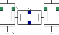
Figure 2: (Color online) Setup of the Josephson charge qubits (green, left and right) coupled by a Josepshon junction (blue, middle). The local charge levels are driven by $E_{J}$. The interaction is driven by $E_{JJ}$.

As an example relating more directly to Eq. (1), we consider two superconducting charge qubits coupled via a Josephson junction Montangero et al. (2007b), as depicted in Fig. 2. The local Hamiltonian reads

$$\boldsymbol{\mathsf{\hat{H}}}^{\text{loc}}_{C} = \sum_{i=1,2}\sum_{n_{i}}\Bigg{[}E_{C}\left(n_{i}-n_{g}^{(i)}\right)^{2}\Ket{n_{i}}\!\Bra{n_{i}}$$ (10)

$$-\frac{E_{J}^{(i)}(t)}{2}\bigg{(}\Ket{n_{i}}\!\Bra{n_{i}+1}+\Ket{n_{i}+1}\!\Bra{n_{i}}\bigg{)}\Bigg{]}\,.$$

We can control the Josephson coupling $E_{j}^{(1)}(t)=E_{j}^{(2)}(t)$, while the charging energy $E_{C}$ and the offset charge $n_{g}^{(i)}$ are fixed. In order to make the connection to Eq. (1) explicit, we truncate each anharmonic ladder to two levels,

$$\boldsymbol{\mathsf{\hat{H}}}^{\text{loc}}_{C,2l}=\sum_{i=1}^{2}\left[E_{C}\left(n_{g}-\frac{1}{2}\right)\boldsymbol{\mathsf{\hat{\sigma}}}_{z}^{(i)}-\frac{E_{J}(t)}{2}\boldsymbol{\mathsf{\hat{\sigma}}}_{x}^{(i)}\right]\,,$$ (11)

omitting terms proportional to the identity. As was shown in Paper I Watts et al. (2014), only a two-dimensional subsection of the Weyl chamber can be reached at the degeneracy point, i.e. $n_{g}=\frac{1}{2}$. Here, as we are more interested in the control problem than in its possible experimental realization and thus its robustness against noise, we set $n_{g}=1$, lifting the degeneracy between the qubit levels and ensuring full controllability.

The interaction is described by

$$\boldsymbol{\mathsf{\hat{H}}}_{JJ}=\frac{E_{JJ}(t)}{2}\sum_{n_{1},n_{2}}\left(\Ket{n_{1},n_{2}+1}\!\Bra{n_{1}+1,n_{2}}+h.c.\right)\,,$$ (12)

or

$$\boldsymbol{\mathsf{\hat{H}}}_{JJ,2l}=\frac{E_{JJ}(t)}{4}\left(\boldsymbol{\mathsf{\hat{\sigma}}}_{x}^{(1)}\boldsymbol{\mathsf{\hat{\sigma}}}_{x}^{(2)}+\boldsymbol{\mathsf{\hat{\sigma}}}_{y}^{(1)}\boldsymbol{\mathsf{\hat{\sigma}}}_{y}^{(2)}\right)\,,$$ (13)

if truncated to two levels. Typically, $E_{C}$ takes values between 20 GHz and 200 GHz, and $E_{J}/E_{C}$ is between $0.03$ and $0.5$. Both single and two-qubit gates can be implemented on a picosecond time scale Nakamura et al. (1999); Makhlin et al. (2001); Yamamoto et al. (2003). The two-level truncation of the Hamiltonian is generally only accurate near the charge degeneracy point. For the parameters considered here, higher levels have to be taken into account.

II.3 Two transmon qubits interacting via a cavity

The transmon qubit Koch et al. (2007) is closely related to the charge qubit, but operated in a different parameter regime, $E_{J}\gg E_{C}$. This makes them significantly less anharmonic than typical charge qubits, but more robust with respect to charge noise. The coupling between two transmons is implemented via a shared transmission line resonator (“cavity”). The energy of each transmon qubit transition is denoted by $\omega_{1}$, $\omega_{2}$ for the first (“left”) and second (“right”) transmon, respectively. Higher levels are given as a Duffing oscillator with anharmonicity $\alpha_{1}$, $\alpha_{2}$. Each qubit couples to the cavity with coupling strength $g_{1}$ , $g_{2}$. In the dispersive limit $|\omega_{i}-\omega_{r}|\gg|g_{i}|$ ($i=1,2$) with $\omega_{r}$ the cavity frequency, the cavity can be eliminated and an effective two-transmon Hamiltonian is obtained. The coupling between each transmon and the cavity turns into an effective qubit-qubit coupling,

$$J^{\operatorname{eff}}\approx\frac{g_{1}g_{2}}{(\omega_{1}-\omega_{r})}+\frac{g_{1}g_{2}}{(\omega_{2}-\omega_{r})}\,.$$ (14)

In most current setups, $J^{\operatorname{eff}}\ll|\omega_{2}-\omega_{1}|$, and the two-transmon Hamiltonian can be approximated as Poletto et al. (2012)

$$\boldsymbol{\mathsf{\hat{H}}}_{T} \approx \sum_{i=1,2}\left(\left(\omega_{i}+\frac{\alpha_{i}}{2}\right)\boldsymbol{\mathsf{\hat{b}}}_{i}^{\dagger}\boldsymbol{\mathsf{\hat{b}}}_{i}-\frac{\alpha_{i}}{2}\left(\boldsymbol{\mathsf{\hat{b}}}_{i}^{\dagger}\boldsymbol{\mathsf{\hat{b}}}_{i}\right)^{2}\right)$$ (15)

$$+J^{\operatorname{eff}}\left(\boldsymbol{\mathsf{\hat{b}}}_{1}^{\dagger}\boldsymbol{\mathsf{\hat{b}}}_{2}+\boldsymbol{\mathsf{\hat{b}}}_{1}\boldsymbol{\mathsf{\hat{b}}}_{2}^{\dagger}\right)$$

$$+\Omega(t)\left(\boldsymbol{\mathsf{\hat{b}}}_{1}+\boldsymbol{\mathsf{\hat{b}}}_{1}^{\dagger}+\lambda\boldsymbol{\mathsf{\hat{b}}}_{2}+\lambda\boldsymbol{\mathsf{\hat{b}}}_{2}^{\dagger}\right)\,,$$

where $\Omega(t)$ is the driving field that couples to the cavity. Typical parameters are listed in Table 1.

left qubit frequency	$\omega_{1}$	4.380	GHz
right qubit frequency	$\omega_{2}$	4.614	GHz
left qubit anharmonicity	$\alpha_{1}$	-210	MHz
right qubit anharmonicity	$\alpha_{1}$	-215	MHz
effective qubit-qubit coupling	$J^{\operatorname{eff}}$	-3.0	MHz
relative coupling strength	$\lambda$	1.03

Table 1: Parameters for the transmon Hamiltonian Eq. (15)

.

A Hamiltonian of the form of Eq. (1) is obtained by truncating the higher levels,

$$\boldsymbol{\mathsf{\hat{H}}}_{T,2l} = \frac{\omega_{i}}{2}{\sigma^{(i)}_{z}}+2J^{\operatorname{eff}}\left(\boldsymbol{\mathsf{\hat{\sigma}}}_{x}^{(1)}\boldsymbol{\mathsf{\hat{\sigma}}}_{x}^{(2)}+\boldsymbol{\mathsf{\hat{\sigma}}}_{y}^{(1)}\boldsymbol{\mathsf{\hat{\sigma}}}_{y}^{(2)}\right)+$$ (16)

$$+\Omega(t)\left(\boldsymbol{\mathsf{\hat{\sigma}}}_{x}^{(1)}+\lambda\boldsymbol{\mathsf{\hat{\sigma}}}_{x}^{(2)}\right)\,.$$

Finally, notice that in systems B and C, the assumption that only two qubit levels are populated leading to Eqs. (13) and (16) might not hold in general, however, we present it to make the connection to Eq. (1) and the controllability analysis of Paper I Watts et al. (2014) explicit.

III Optimal control using CRAB

III.1 Perfect entangler functional in $c$-space

A common choice for a fidelity that quantifies whether an obtained gate $U$ corresponds to the target gate $V$ is Palao and Kosloff (2003)

$$F_{\text{sm}}=\frac{1}{4}\left|\operatorname{tr}\left[V^{\dagger}U\right]\right|^{2}\,.$$ (17)

In the context of the geometric theory for two-qubit gates, reviewed in paper I Watts et al. (2014), where arbitrary local transformations are allowed, the generalization of this fidelity can be expressed through the difference of the Weyl chamber coordinates of the obtained gate $U$ and the target point,

$$F_{\operatorname{LEC}}(U)=\cos\frac{\Delta c_{1}}{2}\cos\frac{\Delta c_{2}}{2}\cos\frac{\Delta c_{3}}{2}\,.$$ (18)

This fidelity can also be used as a functional for optimizing towards gates of a given local equivalence class as shown in the preceding paper. Building on the local equivalence class functional, a functional $F_{\operatorname{PE}}$ for the optimization of an arbitrary perfect entangler can be derived. In the Weyl chamber, the perfect entanglers form a polyhedron confined by the three planes

$$c_{1}+c_{2} = \pi/2\,,$$ (19a)

$$c_{2}+c_{3} = \pi/2\,\quad\text{and}$$ (19b)

$$c_{1}-c_{2} = \pi/2\,.$$ (19c)

These planes divide the Weyl chamber into the polyhedron of perfect entanglers and three corners of non-perfect entanglers. Within the perfect entangler polyhedron, the functional is defined to take the value $F_{\operatorname{PE}}\equiv 1$. Outside of the polyhedron, the value of $F_{\operatorname{PE}}$ depends on the region of the Weyl chamber the gate is in,

$$F_{\operatorname{PE}}(U)=\begin{cases}\cos^{2}\frac{c_{U,1}+c_{U,2}-\frac{\pi}{2}}{4}\,,\qquad c_{1}+c_{2}\leq\frac{\pi}{2}\\ \cos^{2}\frac{c_{U,2}+c_{U,3}-\frac{\pi}{2}}{4}\,,\qquad c_{2}+c_{3}\geq\frac{\pi}{2}\\ \cos^{2}\frac{c_{U,1}-c_{U,2}-\frac{\pi}{2}}{4}\,,\qquad c_{1}-c_{2}\geq\frac{\pi}{2}\\ 1\qquad\text{otherwise (inside polyhedron).}\end{cases}$$ (20)

As shown in the preceding paper, both $F_{\operatorname{LEC}}$ and $F_{\operatorname{PE}}$ are not only optimization functionals but have also a nonlocal fidelity interpretation.

Generally, the logical two-qubit subspace is embedded in a larger Hilbert space, such that while the dynamics in the total Hilbert space are unitary, the dynamics in the subspace may not be. In this case, a closest unitary $U$ can be derived from the non-unitary (projected) gate $\tilde{U}$: If $\tilde{U}$ has the singular value decomposition $\tilde{U}=V\Sigma W^{\dagger}$, then the unitary that fulfills $U=\arg\min_{u}\|u-\tilde{U}\|$ is given by $U=VW^{\dagger}$. The local equivalence-class and perfect entangler fidelities then become

$$F_{\operatorname{LEC}}(\tilde{U})=F_{\operatorname{LEC}}(U)-||\tilde{U}-U||\,,$$ (21)

$$F_{\operatorname{PE}}(\tilde{U})=F_{\operatorname{PE}}(U)-||\tilde{U}-U||\,.$$ (22)

These fidelities can be directly used as optimization functionals. The optimization target is then to find $c_{i}$ in such a way that Eqs. (21) and (22) are maximized.

III.2 CRAB algorithm

The chopped random basis (CRAB) algorithm Doria et al. (2011b); Caneva et al. (2011c) is an optimal control tool that allows to optimize quantum operations in cases where it is either not possible or impractical to calculate gradients of the optimization functional. In the present context, it is mathematically unfeasible to calculate gradients of $F_{\operatorname{LEC}}$ and $F_{\operatorname{PE}}$ as given in Eqs. (21), (22) with respect to the states (as needed for the Krotov update formula in Sec IV below), since the functionals depends on the states in a highly non-trivial way.

The central idea of CRAB is the expansion of the control function into a truncated basis using random basis functions Doria et al. (2011b); Caneva et al. (2011c),

$$u(t)=\sum_{i=1}^{n}c_{i}f_{i}(t)\,,$$ (23)

where the set of $f_{i}$ form the truncated basis. We choose $f_{i}(t)=\sin(\omega_{i}t)$ with random $\omega_{i}\in[\frac{2\pi}{T}(i-0.5),\frac{2\pi}{T}(i+0.5)]$. The coefficients $c_{i}$ are optimized by a direct search algorithm, Nelder-Mead downhill simplex in our case.

IV Optimal control using Krotov’s method

IV.1 Perfect entangler functional in $g$-space

For optimal control approaches utilizing gradient information, the capability to take the derivative of the optimization functional with respect to the unitary $U$, or equivalently, with respect to the time-evolved basis states, is required. This is not possible for the functionals in Eqs. (21) and (22). We therefore use an equivalent functional, based not on the Weyl chamber coordinates $c_{1}$, $c_{2}$, $c_{3}$, but on the local invariants $g_{1}$, $g_{2}$, $g_{3}$ Watts et al. (2014).

An appropriate functional to optimize towards gates in a local equivalence class is given by Müller et al. (2011)

$$J_{\operatorname{LI}}(U)=(\Delta g_{1})^{2}+(\Delta g_{2})^{2}+(\Delta g_{3})^{2}\,,$$ (24)

where $\Delta g_{i}$ is the Euclidean distance between local invariant $g_{i}$ of the obtained unitary $U$ and that of the optimal gate $O$. For the perfect entanglers, the functional becomes Watts et al. (2014)

$$\mathcal{D}(U)=g_{3}\sqrt{g_{1}^{2}+g_{2}^{2}}-g_{1}\,.$$ (25)

Both of these functionals take the value zero if the goal is reached. They are thus distance measures, as opposed to the fidelities in Eqs. (21), (22), and they are not restricted to lie within the range $[0,1]$.

Again, non-unitarity due to projection onto the logical subspace must be taken into account. However, the expression $||\tilde{U}-U||$, similarly to the functionals $F_{\operatorname{LEC}}$, $F_{\operatorname{PE}}$ used in Sec III, cannot easily be differentiated. As an alternative, we minimize the loss of population $\operatorname{tr}\left[\tilde{U}^{\dagger}\tilde{U}\right]/4$ from the logical subspace,

$$J_{\operatorname{LI}}(\tilde{U}) = wJ_{\operatorname{LI}}(U)+(w-1)\left(1-\frac{1}{4}\operatorname{tr}\left[\tilde{U}^{\dagger}\tilde{U}\right]\right)$$ (26)

$$\mathcal{D}(\tilde{U}) = w\mathcal{D}(U)+(w-1)\left(1-\frac{1}{4}\operatorname{tr}\left[\tilde{U}^{\dagger}\tilde{U}\right]\right)\,.$$ (27)

In Eqs. (26), (27), the factor $w\in[0,1]$ is used to weight the relative importance of Weyl-chamber optimization and unitarity. It can adaptively be changed during the optimization in order to improve convergence.

IV.2 Krotov’s Method

In Krotov’s method, the total functional $J$ must include a control-dependent running cost in order to derive an update equation. $J$ takes the form

$$J=J_{T}\left[\{\varphi_{k}(T)\}\right]+\int_{0}^{T}\frac{\lambda_{a}}{S(t)}\left[u(t)-u_{\mathrm{ref}}(t)\right]^{2}\;dt\,,$$ (28)

where $J_{T}$ is a final-time functional, e.g. Eq. (26) or (27). The second term is a constraint on the optimized control field $u(t)$. Taking the reference field $u_{\mathrm{ref}}(t)$ to be the field from the previous iteration ensures that close to the optimum the functional is improved only due to changes in the actual target $J_{T}$ Palao and Kosloff (2003).

A comprehensive description of Krotov’s method for quantum control problems is found in Ref. Reich et al. (2012). Here, we state the control equations for a final-time functional $J_{T}$ that depends higher than quadratically on the states, linear coupling to the control and linear equations of motion. In this case, the update equation for the control at the $i+1$st iterative step, $u^{(i+1)}(t)$, is given by

$$u^{(i+1)}(t)=u_{\mathrm{ref}}(t)+\frac{S(t)}{\lambda}\mathfrak{Im}\bigg{\{}\sum_{k=1}^{4}\left\langle\chi_{k}^{(i)}(t)\Bigg{|}\frac{\partial\boldsymbol{\mathsf{\hat{H}}}}{\partial u}\bigg{|}_{u^{(i+1)}}\Bigg{|}\varphi_{k}^{(i+1)}(t)\right\rangle+\frac{1}{2}\sigma(t)\sum_{k=1}^{4}\left\langle\Delta\varphi_{k}(t)\Bigg{|}\frac{\partial\boldsymbol{\mathsf{\hat{H}}}}{\partial u}\bigg{|}_{u^{(i+1)},}\Bigg{|}\varphi_{k}^{(i+1)}(t)\right\rangle\bigg{\}}$$ (29)

with $\Ket{\Delta\varphi_{k}(t)}=\Ket{\varphi_{k}^{(i+1)}(t)}-\Ket{\varphi_{k}^{(i)}(t)}$ representing the change in state $\Ket{\varphi_{k}(t)}$. In Eq. (29), $S(t)$ is a shape function to smoothly switch the control on and off, and $\lambda$ is a parameter that determines the step size of the change in the control. The scalar function $\sigma(t)$ is constructed to ensure monotonic convergence. For final-time functionals that depend higher than quadratically on the states $|\varphi_{k}(T)\rangle$, linear equations of motion and linear coupling to the control, it reads Reich et al. (2012)

$$\sigma(t)=-\bar{A}$$ (30)

with $\bar{A}=\max\left(\varepsilon_{A},2A+\varepsilon_{A}\right)$, where $\varepsilon_{A}$ is a small non-negative number that can be used to enforce strict inequality in the second order optimality condition. The parameter $A$ depends on the final-time functional. In principle, it is possible to determine a supremum for $A$ that guarantees convergence. In practice, one should determine the optimal value for $A$ in each iteration numerically Reich et al. (2012),

$$A^{(i+1)} = \frac{\sum_{k=1}^{4}\left[\Braket{\chi_{k}\left(T\right)}{\Delta\varphi_{k}\left(T\right)}+\Braket{\Delta\varphi_{k}\left(T\right)}{\chi_{k}\left(T\right)}\right]+J_{T}\left(\{\varphi_{k}^{(i+1)}(T)\}\right)-J_{T}\left(\{\varphi_{k}^{(i)}(T)\}\right)}{\sum_{k=1}^{4}\left[\Braket{\Delta\varphi_{k}\left(T\right)}{\Delta\varphi_{k}\left(T\right)}\right]}\,.$$ (31)

Evaluation of the update equation for the control, Eq. (29), implies forward propagation of the logical basis states and backward propagation of the adjoint states. The forward propagation of the logical basis uses the new control, as indicated by the superscript $(i+1)$,

$$\frac{d}{dt}|\varphi^{(i+1)}_{k}(t)\rangle = -\frac{i}{\hbar}\boldsymbol{\mathsf{\hat{H}}}[u^{(i+1)}]|\varphi^{(i+1)}_{k}(t)\rangle$$ (32a)

$$|\varphi^{(i+1)}_{k}(0)\rangle = |k\rangle\,,\quad k=1,\ldots,4\,.$$ (32b)

The adjoint states are propagated backward in time under the old control, $u^{(i)}$,

$$\frac{d}{dt}|\chi^{(i)}_{k}(t)\rangle = -\frac{i}{\hbar}\boldsymbol{\mathsf{\hat{H}}}^{\dagger}[u^{(i)}]|\chi^{(i)}_{k}\rangle$$ (33a)

$$|\chi^{(i)}_{k}(T)\rangle = -\nabla_{\Bra{\varphi_{k}}}J_{T}\big{|}_{|\varphi^{(i)}_{k}(T)\rangle}\,$$ (33b)

for the $k=1\dots 4$ states that constitute the logical two-qubit basis. Note that it is Eq. (33b) that necessitates a functional that is differentiable with respect to the states. The initial condition for the adjoint states is given in terms of the final-time functional, $J_{T}$. We use either one of the functionals in Eqs. (26) and (27).

V Applications

V.1 Optimization for NV centers in diamond

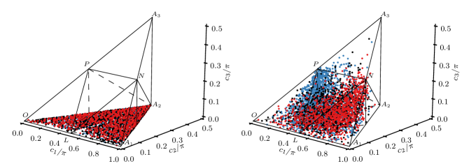
Figure 3: (Color online) Gates reached for an NV center in diamond with 2 control pulses (left) and 3 control pulses (right) during an optimization towards a perfect entangler (black), and towards the equivalence class of the points $P$ and $N$ in the Weyl chamber (blue and red, respectively).

For a system whose dynamics do not leak out of the logical subspace, such as NV centers in diamond introduced in Section II.1, optimization towards a perfect entangler is a powerful tool, given that half of all possible two-qubit gates are perfect entanglers. Since without leakage any control is guaranteed to yield a fully unitary gate, the likelihood of finding a perfect entangler already with an arbitrary control is large, provided the gate duration is sufficiently long.

In Fig. 3, a sampling of all the gates obtained during an optimization of the Hamiltonian (4) is shown, for two pulses, $\Omega_{MW}(t)$ and $\Omega_{RF(t)}$ (left), cf. Eqs. (5) and (6), as well as for a third control $\Delta(t)$ (right), cf. Eq. (9). The gates from an optimization towards the polyhedron of perfect entanglers, using the functional of Eq. (22), are indicated by black dots. The optimization was performed using the CRAB algorithm and was allowed to continue even after reaching a perfect entangler. Furthermore, an optimization towards the local equivalence class of the points $P$ and $N$ (which are corners of the polyhedron of perfect entanglers – see Paper I Watts et al. (2014) for interpretation) using the functional of Eq. (21), encountered the gates shown by blue and red dots, respectively. In all cases, the results confirm the predictions of Section II.1: for two controls all gates lie in the ground plane of the Weyl chamber, whereas for three controls every part of the Weyl chamber is reached.

Since $P$ and $N$ are not reachable using only two control fields, the optimization only yields success for the PE-functional, within at most two iterations. Nonetheless, the gates obtained from all optimization targets (that is PE-functional and the local equivalence classes P and N) sample the entire reachable region; the black, red, and blue points in Fig. 3 (left) each evenly cover the entire ground plane of the Weyl chamber.

For three controls, the system shows full controllability, and the gates from different optimization targets cluster in different regions. The gates from the PE optimization evenly fill most of the front half of the PE polyhedron, whereas the local-equivalence-class optimizations cluster in the direction of their respective target points. In all cases, the desired target is reached. However, there is a dramatic difference in the effort required in the different cases. For the perfect entanglers, the optimization target was reached within usually one or two optimization steps. In contrast, for the optimization towards the $P$ and $N$ points, at least several hundred iterations were necessary.

V.2 Optimization for Josephson Charge Qubits

The optimization problem becomes more difficult once the model accounts for the possibility of leakage out of the logical subspace, which is the case for superconducting qubits. As a first example, we optimize the system of coupled charge qubits described in Sec. II.2, using the CRAB algorithm. For each qubit, six levels were taken into account, and thus leakage from the logical subspace had to be considered, cf. Eqs. (21) and (22).

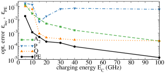
Figure 4: (Color online) Success of optimization for two Josephson charge qubits coupled by a Josephson junction. Control with one pulse $E_{J}(t)=E_{JJ}(t)$ and total time $T=1\,$ns. The error $\varepsilon_{\operatorname{PE}}$ for optimization toward the polyhedron of perfect entanglers (PE) is compared to the error $\varepsilon_{\operatorname{LEC}}$ for optimization towards the local equivalence classes of different points in the Weyl chamber $A_{2}$, $P$, and $Q$.

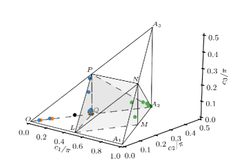
Figure 5: (Color online) Optimized gates in the Weyl chamber, for optimization of two coupled charge qubits with $E_{J}(t)=E_{JJ}(t)$ and total time $T=1\,$ns, using the PE functional as well as the local invariants functional for the points $A$, $P$, $Q$. The end points of the optimization for the results shown in Fig. 4 are indicated, using the same color coding (black for PE optimization, green for optimization towards the $A$ point, blue for $P$, and orange for $Q$).

First, we consider the case $E_{JJ}(t)=E_{J}(t)$, i.e. using only a single control pulse. Figure 4 shows the optimization results of the perfect entanglers functional for different values of $E_{C}$ and compares it to optimization towards a specific perfect entangler equivalence class, for three corners of the polyhedron, $Q$, $A_{2}$, and $P$. Success is measured by the error $\varepsilon_{\operatorname{PE}}(\tilde{U})=1-F_{\operatorname{PE}}(\tilde{U})$ for optimization towards the polyhedron of perfect entanglers (black solid line, circles), and equivalently, $\varepsilon_{\operatorname{LEC}}(\tilde{U})=1-F_{\operatorname{LEC}}(\tilde{U})$ for optimization towards a local equivalence class. Larger values of $E_{C}$ increase the spacing between levels and thus make the implementation of a gate easier as leakage of population to higher levels is suppressed. We stress that while for the truncated Hamiltonian we can show full controllability, this does not clearly imply full controllability also when additional levels are included. Furthermore, the choice of specific parameters can make certain parts of the Weyl chamber harder to reach in the chosen total time. This is indeed what we see and report in Fig. 4: the optimization for an arbitrary perfect entangler significantly outperforms the optimization towards a specific local equivalence class. Indeed, we find that while $Q$ and $A_{2}$ can be reached with an error $\varepsilon_{\operatorname{LEC}}<10^{-3}$ and decreasing with the gate duration (or equivalently increasing $E_{C}$), $P$ cannot be reached with precision higher than a few percent. This finding is supported by Fig. 5 that shows the position in the Weyl chamber of the gates reached during optimization. Each dot corresponds to a reached gate at final time (if leakage is present, the closest gate $\in SU(4)$ is shown; see section III). This explains the blue dot appearing near the point $P$: While the projection onto $SU(4)$ gets relatively close to $P$, a loss of population from the logical subspace of 2.1% is observed, making the overall fidelity low. In contrast, the population loss for the gates ($Q$, $A_{2}$) as well as the perfect entanglers is less then 0.1%. Interestingly, all optimizations towards a perfect entangler cluster around the $Q$ point, which is the point that was reached with highest fidelity by a direct local equivalence class optimization.

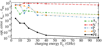
Figure 6: (Color online) Same as Fig. 4 but control with two independent pulses $E_{J}(t)$ and $E_{JJ}(t)$.

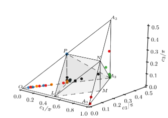
Figure 7: (Color online) Same as Fig. 5 but control with 2 pulses $E_{J}(t)$ and $E_{JJ}(t)$. Color coding as in Fig. 6.

Finally, we relax the constraint $E_{JJ}(t)=E_{J}(t)$, allowing for two independent pulses: Figure 6 shows the optimization success of the perfect entanglers functional for different gate durations, comparing it to optimization towards a given local equivalence class. Here, we examine four corners of the polyhedron, namely $Q$, $A_{2}$, $P$, and also $N$. As expected, again the smallest errors, i.e., highest fidelities, are obtained for perfect entangler optimization. In addition to $Q$ and $A_{2}$, now also $P$ could be implemented with high fidelity, but $N$ (data not included in Fig. 4) remains unreachable. This is also supported by Fig. 7 that shows the position in the Weyl chamber of the gates reached during optimization. The obtained results for two independent pulses suffer from significantly less loss of population from the logical subspace compared to optimization with a single pulse. This is the expected behavior as the system goes from being weakly controllable (the drift Hamiltonian is needed to counteract leakage) for one control to being fully controllable for two controls Motzoi et al. (2009). For the optimization towards specific points in the Weyl chamber, the loss was below 0.01%, for the perfect entanglers it was as low as machine precision.

V.3 Optimization of Transmon Qubits

Lastly, for two transmons as described in Sec. II.3, we analyze the performance of the perfect entanglers functional using Krotov’s method, outlined in Sec. IV. The optimization is carried out for different gate durations between 25 ns and 400 ns, starting from a $\sin$-squared guess pulse of 35 MHz peak amplitude.

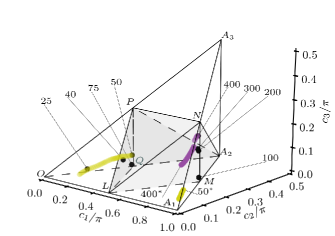
Figure 8: (Color online) Optimized gates in the Weyl chamber, for two transmon qubits, optimized with Krotov’s method for the perfect entangler functional in Eq. (27). The point at which each optimization enters the PE polyhedron, or the end point of the optimization if no PE can be achieved, is shown by a black dot and labeled with the gate duration. The entire optimization paths for $T=50\,$ns and $T=400\,$ns are shown in light blue and dark purple, respectively, with the starting points labeled by 50^∗ and 400^∗.

Figure 8 shows the results of the optimization in the Weyl chamber. The point at which each optimization enters the perfect entanglers polyhedron is indicated by a black dot and labeled with the gate duration. For $T<50\,$ns, no perfect entangler can be reached – defining heuristically the QSL for this transformation. In order to illustrate how the optimization proceeds, the optimization paths for $T=50\,$ns, i.e., the gate at the QSL, and a high-fidelity gate ($T=400\,$ns) are traced in light blue and dark purple, respectively. Both optimizations start in the $W_{0}^{*}$ region (near the $A_{1}$ point). The gate obtained with the guess pulse for $T=50\,$ns is significantly farther away from the surface of the polyhedron of PE than that for the guess pulse with $T=400\,$ns. Optimization for $T=400\,$ns therefore moves directly towards the $W_{0}^{*}$ surface of the PE polyhedron, whereas the optimization for $T=50$ ns enters the ground plane and emerges in the $W_{0}$ region, before finally reaching the $W_{0}$ surface of the polyhedron of perfect entanglers. The jump from $W_{0}^{*}$ to $W_{0}$ is indicated by the light blue arrow. We find the optimization to enter $W_{0}$ from $W_{0}^{*}$ for durations $<100\,$ns, whereas for longer gate duration the optimizations stay within $W_{0}^{*}$ entirely. The different optimization paths are a result of the competition between the two objectives – to reach a perfect entangler, and to implement a gate that is unitary in the logical subspace (the points shown in Fig. 8 are the Weyl chamber coordinates of the unitary $U$ closest to the actual time evolution $\tilde{U}$). The latter objective is more difficult to realize for shorter gate durations, resulting in a more indirect approach to the polyhedron of perfect entanglers than one might expect when considering that objective alone.

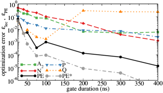
Figure 9: (Color online) Comparison of optimization success for the PE functional compared to the local invariants (LI) functional for several points in the Weyl chamber. The optimization success using Krotov’s method is measured in $c$-space, although the optimization functionals are defined in $g$-space (see text for details). For the LI-optimization, the results are fully converged. For the PE-optimization, the results are converged to a relative change below $10^{-2}$ (black solid curve) and $10^{-3}$ (gray dash-dash-dotted curve).

Analogously to the study of charge qubit optimization in Sec. V.2, it is instructive to compare the optimization success of the perfect entangler functional, Eq. (27), to that of the local invariants functional, Eq. (26), for a few select points of the Weyl chamber. This is shown in Fig. 9. Instead of the optimization functionals Eqs. (27) and (26) we plot the gate errors $1-F_{\operatorname{LEC}}(\tilde{U})$ for the local invariants optimization, and $1-F_{\operatorname{PE}}(\tilde{U})$ for the PE optimization, see. Eqs. (21) and (22).

The results of Fig. 9 show how, for different gate durations, the gates that are easiest to reach differ. In agreement with the results of Fig. 8, for durations $<50$ ns, the jump in the optimization error indicates a speed limit. For short gate durations, $50~{}\text{ns}\leq T\leq 100~{}\text{ns}$, optimization towards the point $Q$ in the Weyl chamber is most successful. This matches the optimized gates for $T\leq 100\,$ns in Fig. 8 being near the $Q$ point. Also correspondingly, the longer gate durations end near the $N$ point. The failure to reach the point $Q$ for longer durations is due to the symmetry structure of the Weyl chamber. Namely, for the ground plane of the chamber, there is a mirror axis defined by the line through $L$ and $A_{2}$, where mirrored points are in the same local equivalence class. Both the $Q$-point and the $M$ point have local invariants of $g_{1}=\frac{1}{4},g_{2}=0,g_{3}=1$. Since the optimization was performed in $g$-space, these two points are not distinguishable; indeed, for long gate durations, the $Q$-optimization successfully reached the $M$ point.

In comparison with the local invariants optimization, the perfect entanglers functional shows excellent performance. It automatically identifies the optimal gate for a given gate duration and reaches significantly better fidelities. This is due to the fact that the desired entangling power of $U$ can usually be obtained in just a few tens of iterations of the algorithm, and the remainder of the optimization then focuses on improving the unitarity of the obtained gate $\tilde{U}$. Most strikingly, we find that for the optimization towards a specific local equivalence class, the convergence rate becomes extremely small as the optimum is approached. All the results shown in Fig. 9 are converged to a relative change below $10^{-4}$, such that no measurable improvement can be expected within a reasonable number of iterations. While in principle (due to the full controllability of the system), the direct optimizations should yield arbitrarily small gate errors, as long as the gate duration is above the quantum speed limit, in practice this depends on numerical parameters such as the weight $\lambda_{a}$ in Krotov’s method and may take a extremely large number of iterations or stagnate, as we observe here. The perfect entangler optimization shows remarkable robustness with respect to this issue. We observed very little slow-down in convergence. The black curve in Fig. 9 for the PE-optimization already yields a significantly smaller optimization error than any of the LI-optimizations, but is only converged to a relative change of $10^{-2}$. Even the gray dash-dash-dotted curve, labeled PE^∗, is only converged to a relative change of $10^{-3}$, and thus the optimization would still yield considerably better results if it were to be continued.

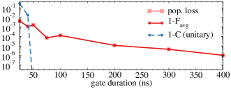
Figure 10: (Color online) Analysis of the sources of error for PE of 2 transmon qubits: Population loss from the logical subspace (light red squares), concurrence error of the closest unitary gate $U$ in the logical subspace (blue circles), and average gate error, $\varepsilon_{avg}=1-F_{avg}$, with which $U$ is implemented (red circles).

The values of the optimization error in Fig. 9 of $10^{-3}$ or $10^{-2}$ should not be understood to indicate a gate error above the quantum error correction threshold. Whereas the optimization error relates only to a figure of merit used for optimization, the relevant physical quantity that would be determined in an experiment is the average gate fidelity. It can be evaluated as Pedersen et al. (2007)

$$F_{avg} = \frac{1}{20}\sum_{i,j=1}^{4}\bigg{(}\langle\varphi_{i}|\boldsymbol{\mathsf{\hat{O}}}^{\dagger}\boldsymbol{\mathsf{\hat{U}}}\Ket{\varphi_{i}}\!\Bra{\varphi_{j}}\boldsymbol{\mathsf{\hat{U}}}^{\dagger}\boldsymbol{\mathsf{\hat{O}}}|\varphi_{j}\rangle$$ (34)

$$+\operatorname{tr}\left[\boldsymbol{\mathsf{\hat{O}}}\Ket{\varphi_{i}}\!\Bra{\varphi_{i}}\boldsymbol{\mathsf{\hat{O}}}^{\dagger}\boldsymbol{\mathsf{\hat{U}}}\Ket{\varphi_{j}}\!\Bra{\varphi_{j}}\boldsymbol{\mathsf{\hat{U}}}^{\dagger}\right]\bigg{)}\,,$$

assuming a two-qubit target gate $\boldsymbol{\mathsf{\hat{O}}}$ and denoting the logical basis by $\{\Ket{\varphi_{i}}\}$. Figure 10 shows the generated entanglement as measured by the concurrence and the average gate error, $\varepsilon_{avg}=1-F_{avg}$, together with the population loss from the logical subspace. $\boldsymbol{\mathsf{\hat{O}}}$ is taken to be the unitary that is closest to the projection of the realized operation from the full Hilbert space onto the logical subspace. For $T>50\,$ns, the gate errors are at or below $10^{-4}$. For shorter gate durations, insufficient entanglement is generated, cf. blue dashed curve in Fig. 10. Once $T$ is sufficiently large to generate the desired entanglement, the only source of error is loss of population from the logical subspace, shown in light red in Fig. 10. This loss does not depend on the choice of the weight $w$ in Eq. (27). When the gate duration is increased, optimization yields gates that are exponentially more unitary, as indicated by the linear decrease of the average gate error in our semi-log plot, in agreement with recently introduced error bounds for optimal transformations Lloyd and Montangero (2014). The difficulty to ensure unitarity on the logical subspace is typical for weakly anharmonic ladders, as found in superconducting transmon or phase qubits. Optimal control can be successfully employed to tackle the problem of ensuring unitarity in the logical subspace, in addition to generating entanglement, as exemplified in Fig. 10.

VI Conclusions

We have employed an optimization functional targeting an arbitrary perfect entangler to obtain gate implementations for NV centers in diamond and superconducting Josephson junctions. For NV centers in diamonds, to a good approximation, the dynamics is confined to the logical subspace. In this case, optimization for a perfect entangler turns out to be trivial. This finding is in striking contrast to optimization for a specific local equivalence class which requires a large number of iterations, if it is successful at all. The ease with which perfect entanglers are identified for perfectly unitary time evolution can be rationalized by the fact that more than half of all non-local two-qubit gates are perfect entanglers.

When population may leak out of the logical subspace, the optimization problem becomes more difficult. Our corresponding examples were the anharmonic ladders of superconducting qubits in the charge and transmon architectures. While an optimization for a perfect entangler is then no longer trivial, it converges much faster than an optimization for a local equivalence class. This is rationalized by the larger flexibility that a functional offers which allows for more possible solutions. Larger flexibility implies an easier optimization problem, which is reflected in better convergence properties of the algorithm, i.e., optimization is less likely to get stuck, and better final gate fidelities can be reached. The perfect entanglers functional is thus a better tool to investigate the quantum speed limit for perfectly entangling two-qubit gates, i.e., the minimum time in which an perfectly entangling gate operation can be performed, than the local invariants functional.

We find a qualitatively similar performance of two variants of the perfect entanglers functional, expressed in terms of the Weyl chamber coordinates and the local invariants. This is despite the very different topologies connected with each formulation.

Our results underline the importance of properly expressing the physical target in an optimization functional. This is particularly encouraging in view of more complex quantum systems than those considered here, including models that explicitly account for decoherence. Such applications require identification of the unitary that is closest to the actual dynamical map in order to evaluate the perfect entanglers functional. This is possible by extending the mathematical framework developed in Refs. Goerz et al. (2014b); Reich et al. (2013) and will be subject of future work.