Non-equilibrium Berezinskii-Kosterlitz-Thouless Transition in a Driven Open Quantum System

The Berezinskii-Kosterlitz-Thouless mechanism, in which a phase transition is mediated by the proliferation of topological defects, governs the critical behaviour of a wide range of equilibrium two-dimensional systems with a continuous symmetry, ranging from superconducting thin films to two-dimensional Bose fluids, such as liquid helium and ultracold atoms. We show here that this phenomenon is not restricted to thermal equilibrium, rather it survives more generally in a dissipative highly non-equilibrium system driven into a steady-state. By considering a light-matter superfluid of polaritons, in the so-called optical parametric oscillator regime, we demonstrate that it indeed undergoes a vortex binding-unbinding phase transition. Yet, the exponent of the power-law decay of the first order correlation function in the (algebraically) ordered phase can exceed the equilibrium upper limit – a surprising occurrence, which has also been observed in a recent experiment Roumpos et al. (2012). Thus we demonstrate that the ordered phase is somehow more robust against the quantum fluctuations of driven systems than thermal ones in equilibrium.

The Hohenberg-Mermin-Wagner theorem prohibits spontaneous symmetry breaking of continuous symmetries and associated off-diagonal long-range order for systems with short-range interactions at thermal equilibrium in two (or fewer) dimensions Mermin and Wagner (1966). This is because long-range fluctuations due to the soft Goldstone mode are so strong as to be able to “shake apart” any possible long-ranged order. The Berezinskii-Kosterlitz-Thouless (BKT) mechanism (for an overview see Refs. Chaikin and Lubensky (2000); Minnhagen (1987)) provides a loophole to the Hohenberg-Mermin-Wagner theorem: Two-dimensional (2D) systems can still exhibit a phase transition between a quasi-long-range ordered phase below a critical temperature, where correlations decay algebraically and topological defects are bound together, and a disordered phase above such a temperature, where defects unbind and proliferate, causing exponential decay of correlations. Further, it can be shown Nelson and Kosterlitz (1977) that the algebraic decay exponent in the ordered phase cannot exceed the upper bound value of $1/4$.

The BKT transition is relevant for a wide class of systems, perhaps the most celebrated examples are those in the context of 2D superfluids, as in ⁴He and ultracold atoms: Here, despite the absence of true long-range order, as well as a true condensate fraction, clear evidence of superfluid behaviour has been observed in the ordered phase Bishop and Reppy (1978). Particularly interesting, and far from obvious, is the case of harmonically trapped ultracold atomic gases Hadzibabic et al. (2006). While, in an ideal gas, trapping modifies the density of states to allow Bose-Einstein condensation and a true condensate Petrov et al. (2004); Pitaevskii and Stringari (2003), weak interactions change the phase transition from normal-to-BEC to normal-to-superfluid and recover the BKT physics despite the system’s harmonic confinement.

These considerations are applicable to equilibrium, where the BKT transition can be understood in terms of the free energy being minimised in either the phase with free vortices or in the one with bound vortex-anti-vortex pairs. However, in recent years a new class of 2D quantum systems has emerged: strongly driven and highly dissipative interacting many-body light-matter systems such as, for example, polaritons in semiconductor microcavities Carusotto and Ciuti (2013), cold atoms in optical cavities Ritsch et al. (2013) or cavity arrays Carusotto et al. (2009); Hartmann et al. (2008). Due to the dissipative nature of the photonic part, a strong drive is necessary to sustain a non-equilibrium steady-state. In spite of this, a transition from a normal to a superfluid phase in driven microcavity polaritons has been observed Kasprzak et al. (2006); Deng et al. (2010), and the superfluid properties of the ordered phase have started being explored Amo et al. (2009a, b); Sanvitto et al. (2010); Marchetti et al. (2010); Tosi et al. (2011). Being strongly driven, the system does not obey the principle of free energy minimisation, and so it is not obvious whether the transition between the normal and superfluid phases, as the density of particles is increased, is of the BKT type i.e. due to vortex-antivortex pairs unbinding.

Current experiments are not yet able to resolve single shot measurements, and so are not sufficiently sensitive to detect randomly moving vortices. Algebraic decay of correlations was reported from averaged data Roumpos et al. (2012); Roumpos and Yamamoto (2012), however, the power-law decay displays a larger exponent than is possible in equilibrium, which posed questions as to the actual mechanism of the transition. On the theory side, by mapping the complex Ginzburg-Landau equation describing long-wavelength condensate dynamics onto the anisotropic Kardar-Parisi-Zhang (KPZ) equation, Altman et al. Altman et al. (2013) concluded that although no algebraic order is possible in a truly infinite system, the KPZ length scale is certainly much larger than any reasonable system size in the case of microcavity polaritons.

In this work, we consider the case of microcavity polaritons coherently driven into the optical parametric oscillator regime Stevenson et al. (2000); Baumberg et al. (2000) as the archetype of a 2D driven-dissipative system. Another popular pumping scheme is incoherent injection of hot carriers, which relax down to the polariton ground state by exciton formation and interactions with the lattice phonons Kasprzak et al. (2006); Deng et al. (2010). However, the incoherently pumped polariton system is challenging to model due to the complicated and not yet fully understood processes of pumping and relaxation. As a result, one is typically forced to use phenomenological models Chiocchetta and Carusotto (2014), which often suffer from spurious divergences. From this point of view, the parametric pumping scheme is particularly appealing, as an ab initio theoretical description can be developed in terms of a system Hamiltonian Vogel and Risken (1989), and its predictions can be directly compared to experiment.

Analysing the non-equilibrium steady-state, we show that despite the presence of a strong drive and dissipation the transition from the normal to the superfluid phase in this light-matter interacting system is of the BKT type i.e governed by binding and dissociation of vortex-antivortex pairs as a function of particle density, and bares a lot of similarities to the equilibrium counterpart. However, as recent experiments suggested Roumpos et al. (2012), we find that larger exponents of the power-law decay are possible before vortices unbind and destroy the quasi-long-range order leading to exponential decay. This suggests that the external drive, decay and associated noise favours excitations of collective excitations, the Goldstone phase modes, which lead to faster spatial decay, over unpaired vortices which would destroy the quasi-order all together. This externally over-shaken but not stirred quantum fluid constitutes an interesting new laboratory to explore non-equilibrium phases of matter.

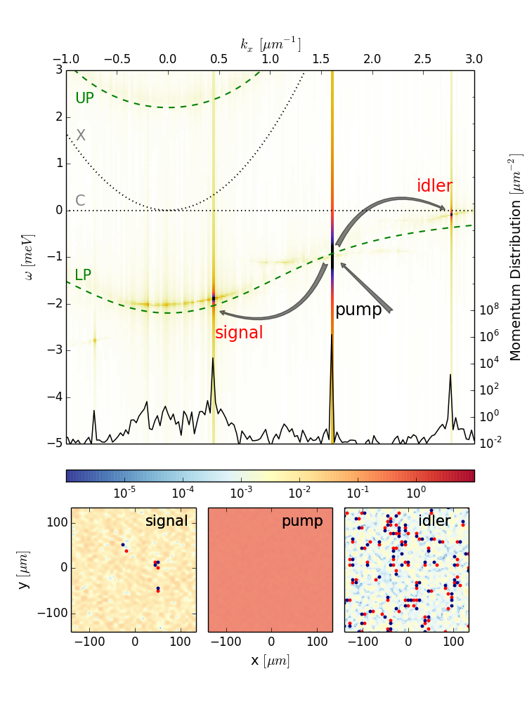
Figure 1: Polariton system in the OPO regime. Upper panel: 2D map of the photonic OPO spectrum $|\psi_{C,k_{x},k_{y}=0}(\omega)|^{2}$ (logarithmic scale) of energy $\omega$ versus the $k_{x}$ momentum component (cut at $k_{y}=0$) for a single noise realisation and at a pump power $f_{p}=1.02436f_{p}^{\text{th}}$, where $f_{p}^{{}^{\textrm{th}}}$ is the mean-field OPO threshold. The arrows show schematically the parametric process scattering polaritons from the pump state into the signal and idler modes. Dashed (green) lines show the bare upper (UP) and lower polariton (LP) dispersions, while dotted (black) lines are the cavity photon ($C$) and exciton ($X$) dispersions. The solid (black) line underneath the spectrum is the $k_{y}=0$ cut of the single-shot time-averaged in the steady-state momentum distribution $\int dt|\psi_{C,k_{x},k_{y}=0}(t)|^{2}$, clearly showing the macroscopic occupation of the three OPO pump, signal, and idler states. Lower panels: 2D maps of the filtered space profiles $|\psi_{s,p,i}({\mathbf{r}},t)|^{2}$ at a fixed time $t$ for which a steady-state regime is reached — the pump emission intensity is rescaled to $1$. Blue (red) dots indicate the vortex (antivortex) core positions.

Simulating driven-dissipative open systems

We describe the dynamics of polaritons in the OPO regime, including the effects of fluctuations, by starting from the system Hamiltonian for the coupled exciton and cavity photon field operators $\hat{\psi}_{X,C}({\mathbf{r}},t)$, depending on time $t$ and 2D spatial coordinates ${\mathbf{r}}=(x,y)$ ($\hbar=1$):

$$\hat{H}_{S}=\int d{\mathbf{r}}\begin{pmatrix}\hat{\psi}_{X}^{{\dagger}}&\hat{\psi}_{C}^{{\dagger}}\end{pmatrix}\begin{pmatrix}\frac{-\nabla^{2}}{2m_{X}}+\frac{g_{X}}{2}|\hat{\psi}_{X}|^{2}&\frac{\Omega_{R}}{2}\\ \frac{\Omega_{R}}{2}&\frac{-\nabla^{2}}{2m_{C}}\end{pmatrix}\begin{pmatrix}\hat{\psi}_{X}\\ \hat{\psi}_{C}\end{pmatrix}\;.$$

Here, $m_{X,C}$ are the exciton and photon masses, $g_{X}$ the exciton-exciton interaction strength, and $\Omega_{R}$ the Rabi splitting Carusotto and Ciuti (2013). In order to introduce the effects of both an external drive (pump) and the incoherent decay, we add to $\hat{H}_{S}$ a system-bath Hamiltonian $\hat{H}_{SB}$

$$\hat{H}_{SB}=\int d{\mathbf{r}}\left[F({\mathbf{r}},t)\hat{\psi}_{C}^{{\dagger}}({\mathbf{r}},t)+\text{H.c.}\right]\\ +\sum_{{\mathbf{k}}}\sum_{l=X,C}\left\{\zeta^{l}_{{\mathbf{k}}}\left[\hat{\psi}_{l,{\mathbf{k}}}^{{\dagger}}(t)\hat{B}_{l,{\mathbf{k}}}+\text{H.c.}\right]+\omega_{l,{\mathbf{k}}}\hat{B}_{l,{\mathbf{k}}}^{{\dagger}}\hat{B}_{l,{\mathbf{k}}}\right\}\;,$$

where $\hat{\psi}_{l,{\mathbf{k}}}(t)$ are obtained Fourier transforming to momentum space ${\mathbf{k}}=(k_{x},k_{y})$ the corresponding field operators in real space $\hat{\psi}_{l}({\mathbf{r}},t)$. $\hat{B}_{l,{\mathbf{k}}}$ and $\hat{B}_{l,{\mathbf{k}}}^{{\dagger}}$ are the bath’s bosonic annihilation and creation operators with momentum ${\mathbf{k}}$ and energy $\omega_{l,{\mathbf{k}}}$, describing the decay processes for both excitons and cavity photons. To compensate the decay, the system is driven by an external homogeneous coherent pump $F({\mathbf{r}},t)=f_{p}e^{i({\mathbf{k}}_{p}\cdot{\mathbf{r}}-\omega_{p}t)}$, which continuously injects polaritons into a pump state, with momentum ${\mathbf{k}}_{p}$ and energy $\omega_{p}$.

Within the Markovian bath regime, standard quantum optical methods Szymańska et al. (2007); Walls and Milburn (2007) can be used to eliminate the environment and obtain a description of the system dynamics in terms of a master equation. As the full quantum problem is, in practice, intractable, a simple yet useful description of the parametric oscillation process properties is provided by the mean-field approximation, where the quantum fields $\hat{\psi}_{l}({\mathbf{r}},t)$ are replaced by the classical fields $\psi_{l}({\mathbf{r}},t)$, whose dynamics is governed by the following generalised Gross-Pitaevskii equation Carusotto and Ciuti (2013)

$$i\partial_{t}\begin{pmatrix}\psi_{X}\\ \psi_{C}\end{pmatrix} =H_{MF}\begin{pmatrix}\psi_{X}\\ \psi_{C}\end{pmatrix}+\begin{pmatrix}0\\ F({\mathbf{r}},t)\end{pmatrix}$$ (1)

$$H_{MF} =\begin{pmatrix}\frac{-\nabla^{2}}{2m_{X}}+g_{X}|\psi_{X}|^{2}-i\kappa_{X}&\frac{\Omega_{R}}{2}\\ \frac{\Omega_{R}}{2}&\frac{-\nabla^{2}}{2m_{C}}-i\kappa_{C}\end{pmatrix}\;,$$

where $\kappa_{X,C}$ are the exciton and photon decay rates. By solving (1) both analytically and numerically, much work has been carried out on the mean-field dynamics for polaritons in the OPO regime and its properties analysed in detail Whittaker (2005); Wouters and Carusotto (2007a); Marchetti and Szymańska (2012). Here, polaritons resonantly injected into the pump state, with momentum ${\mathbf{k}}_{p}$ and energy $\omega_{p}$, undergo parametric scattering into the signal $({\mathbf{k}}_{s},\omega_{s})$ and idler $({\mathbf{k}}_{i},\omega_{i})$ states — see Fig. 1. As explained in detail in Ref. SM , as well as in other works Marchetti and Szymańska (2012), the full steady-state OPO photon emission $\psi_{C}({\mathbf{r}},t)$ is filtered in momentum around the values of the signal, pump and idler momenta ${\mathbf{k}}_{s,p,i}$ in order to get their corresponding steady-state profiles, i.e., $\psi_{s,p,i}({\mathbf{r}},t)=\sum_{|{\mathbf{k}}-{\mathbf{k}}_{s,p,i}|<\tilde{k}_{s,p,i}}\psi_{C,{\mathbf{k}}}(t)e^{i{\mathbf{k}}\cdot{\mathbf{r}}}$. The choice of each state filtering radius, $\tilde{k}_{s,p,i}$, is such that the filtered profiles $\psi_{s,p,i}({\mathbf{r}},t)$ are not affected by them — for details, see SM . The mean-field onset of OPO is shown in the inset of Fig. 3, where the mean-field densities of both pump and signal are plotted as a function of the increasing pump power $f_{p}$. At mean-field level, parametric processes lock the sum of the phases of signal and idler fields $\psi_{s,i}$ to that of the external pump, while allowing a global $U(1)$ gauge symmetry for their phase difference to be spontaneously broken into the OPO phase — a feature which implies the appearance of a Goldstone mode Wouters and Carusotto (2007b). As shown below, fluctuations above mean-field can lift, close to the OPO threshold, this perfect phase locking.

Fluctuations beyond the Gross-Pitaevskii mean-field description (1) can be included by making use of phase-space techniques — for a general introduction, see Ref. Gardiner and Zoller (2004) , while for recent developments in quantum fluids of atoms and photons, see, e.g., Refs. Carusotto and Ciuti (2005); Giorgetti et al. (2007); Foster et al. (2010). Here, the quantum fields $\hat{\psi}_{l}({\mathbf{r}},t)$ are represented as quasiprobability distribution functions in the functional space of C-number fields $\psi_{l}({\mathbf{r}},t)$. Under suitable conditions, the Fokker-Planck partial differential equation, which governs the time evolution of the quasiprobability distribution, can be mapped on a stochastic partial differential equation, which in turn can be numerically simulated on a finite $N\times N$ grid with spacing $a$ (along both $x$ and $y$ directions) and a total size $L_{x,y}=Na$ comparable to the polariton pump spot size in state-of-the-art experiments. For the system under consideration here, the Wigner representation – one of the many possible quasiprobability distributions – is the most suitable to numerical implementation: in the limit $g_{X}/(\kappa_{X,C}dV)\ll 1$, where $dV=a^{2}$ is the cell area, it appears in fact legitimate Drummond and Walls (1980); Vogel and Risken (1989) to truncate the Fokker-Planck equation, retaining the second-order derivative term only, thus obtaining the following stochastic differential equation:

$$id\begin{pmatrix}\psi_{X}\\ \psi_{C}\end{pmatrix}=\left[H_{MF}^{\prime}\begin{pmatrix}\psi_{X}\\ \psi_{C}\end{pmatrix}+\begin{pmatrix}0\\ F\end{pmatrix}\right]dt+i\begin{pmatrix}\sqrt{\kappa_{X}}dW_{X}\\ \sqrt{\kappa_{C}}dW_{C}\end{pmatrix}\;.$$ (2)

Here, $dW_{l=X,C}$ are complex valued, zero-mean, independent Weiner noise terms with $\langle dW^{*}_{l}({\mathbf{r}},t)dW_{m}({\mathbf{r}}^{\prime},t)\rangle=\delta_{{\mathbf{r}},{\mathbf{r}}^{\prime}}\delta_{l,m}\frac{dt}{dV}$, and the operator $H_{MF}^{\prime}$ coincides with $H_{MF}$ in Eq. (1) with the replacement $|\psi_{X}|^{2}\mapsto|\psi_{X}|^{2}-\frac{1}{dV}$. The same stochastic equation (2) can be alternatively derived applying a Keldysh path integral formalism to the Hamiltonian $\hat{H}_{S}+\hat{H}_{SB}$, integrating out the bath fields, and keeping only the renormalisation group relevant terms Sieberer et al. (2013). Note that, remarkably, some of the difficulties of the truncated Wigner method met in the context of equilibrium systems, such as for cold atoms, are suppressed here by the presence of loss and pump terms, i.e., the existence of a small parameter $g_{X}/(\kappa_{l}dV)$ which controls the truncation Carusotto and Ciuti (2013). Note, however, that the bound on this truncation parameter involves the cell area $dV$ of the numerical grid, that is the UV cut-off of the stochastic truncated Wigner equation. For typical OPO parameters, it is possible to choose $dV$ small enough to capture the physics, but at the same time large enough to keep the UV issues under control.

We reconstruct the steady-state Wigner distributions $\psi_{l}({\mathbf{r}},t)$ by considering a monochromatic homogeneous continuous-wave pump $F({\mathbf{r}},t)=f_{p}e^{i({\mathbf{k}}_{p}\cdot{\mathbf{r}}-\omega_{p}t)}$ as before and letting the system evolve to its steady-state. In order to rule out any dependence on the chosen initial conditions, we have considered four extremely different cases: empty cavity with random noise initial conditions and adiabatic increase of the external pump power strength; mean-field condensate initial conditions; either random or mean-field initial conditions in the presence of an unpumped region at the edges of the numerical box, so to model a sort of “vortex-antivortex reservoir. The different initial stage dynamics, and their physical interpretation for each of these four different initial conditions, are carefully described in SM ; in all four cases we always reach the very same steady-state regime, i.e., all noise averaged observable quantities discussed in the following lead to the same result — this could not be a priori assumed for a non-linear system.

Below we first analyse results from single noise realisations (concretely, here, for the case of mean-field initial conditions and no “V-AV reservoir” present), by filtering the photon emission at the signal, pump and idler momenta as also previously done at mean-field level. The filtered profiles are again indicated as $\psi_{s,p,i}({\mathbf{r}},t)$ — for details on filtering see SM . Second, we consider a large number of independent noise realisations and perform stochastic averages of appropriate field functions in order to determine the expectation values of the corresponding symmetrically ordered quantum operators. In particular, we evaluate the signal first-order correlation function as

$$g^{(1)}({\mathbf{r}})=\displaystyle\frac{\langle\psi_{s}^{*}({\mathbf{r}}+{\mathbf{R}},t)\psi_{s}({\mathbf{R}},t)\rangle}{\sqrt{\langle\psi_{s}^{*}({\mathbf{R}},t)\psi_{s}({\mathbf{R}},t)\rangle\langle\psi_{s}^{*}({\mathbf{r}}+{\mathbf{R}},t)\psi_{s}({\mathbf{r}}+{\mathbf{R}},t)\rangle}}\;,$$ (3)

where the averaging $\langle\dots\rangle$ is taken over both noise realisations as well as the auxiliary position ${\mathbf{R}}$, and where $t$ is either a fixed time after a steady-state is reached, or we take additional time average in the steady-state SM .

.1 Vortices and densities across the transition

It is particularly revealing to explore the steady-state profiles, i.e. $\psi_{s,p,i}({\mathbf{r}},t)$, of the signal, pump and idler states. Fig. 1 shows a cut at $k_{y}=0$ of the OPO spectrum, $|\psi_{C,k_{x},k_{y}=0}(\omega)|^{2}$, determined by solving Eq. (2) for $\psi_{X,C}({\mathbf{r}},t)$ to a steady-state and evaluating the Fourier transforms in both space and time. Note, that the logarithmic scale of this 2D map plot (which we employ to clearly characterise all three OPO states) makes the emission artificially broad in energy, while in reality this is sharp (as required by a steady-state regime), as well as it is very narrow in momentum. The filtered space profiles $\psi_{s,p,i}({\mathbf{r}},t)$ shown in the bottom panels of Fig. 1 reveal that while the pump state is homogeneous and free from defects, vortex-antivortex (V-AV) pairs are present for both signal and idler states. Note, that while at the mean-field level the sum of the signal and idler phases is locked to the one of the pump (and thus a V in the signal implies the presence of an AV at the same position in the idler), the large fluctuations occurring in the vicinity of the OPO threshold make this coherent phase-locking mechanism only weakly enforced, resulting in a different number (and different core locations) of V-AV pairs in the signal and idler states. Because the density of photons in the idler state is much lower than the one at the signal (see, e.g., the photonic momentum distribution plotted as a solid black line inside the upper panel of Fig. 1), while both states experience the same noise strength, the number of V-AV pairs in the filtered photonic signal profile is much lower than the number of pairs in the filtered photonic idler profile. Phase locking between signal and idler is recovered instead for pump powers well above the OPO threshold, where long-range coherence over the entire pumping region is re-established.

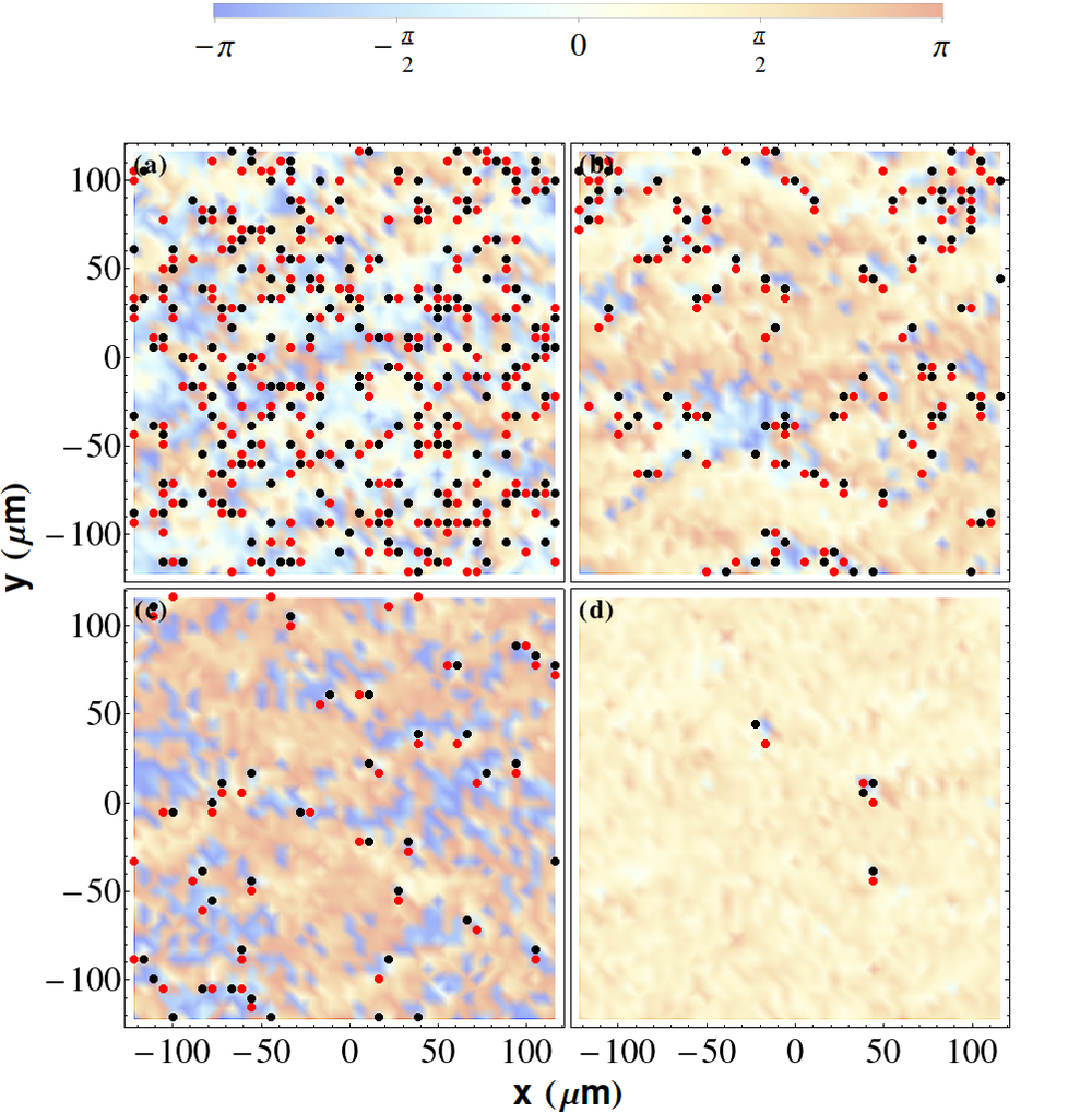
Figure 2: Binding-unbinding transition and vortex-antivortex proliferation across the OPO threshold. Phase (colour map) of the filtered OPO signal $\psi_{s}({\mathbf{r}},t)$ and position of vortices (black dots) and antivortices (red dots) for increasing values of the pump power, in a narrow region close to the mean-field OPO threshold $f_{p}^{\text{th}}$: (a) $f_{p}=1.00287f_{p}^{\textrm{th}}$, (b) $f_{p}=1.01648f_{p}^{\textrm{th}}$, (c) $f_{p}=1.01719f_{p}^{\textrm{th}}$, and (d) $f_{p}=1.02436f_{p}^{\textrm{th}}$. We observe a dramatic decrease of both the number of Vs and AVs, as well as the typical distance between pairs, as a function of the increasing pump power. The filtered profiles are plotted at a late stage of the dynamics, at which a steady-state is reached.

The proliferation of vortices below the OPO transition, followed by a sharp decrease in their density and their binding into close vortex-antivortex pairs is illustrated in Fig. 2. Here, we plot the 2D maps of the phase for the single noise realisation of the filtered OPO signal $\psi_{s}({\mathbf{r}},t)$ (photonic component) for increasing values of the pump power $f_{p}$ in a narrow region close to the mean-field OPO threshold $f_{p}^{\text{th}}$; the position of the generated vortices (antivortices) are marked with blue (black) dots. While at lower pump powers there is a dense “plasma” of Vs and AVs, the number of V-AV pairs decrease with increasing pump powers till eventually disappearing altogether (not shown). We do also record a net decrease in the distance between nearest neighbouring vortices with opposite winding number with respect to that between vortices with the same winding number. In order to quantify the vortex binding across the OPO transition, we measure, for each detected vortex, the distance to its nearest vortex, $r_{\text{V-V}}$ and to its nearest antivortex $r_{\text{V-AV}}$; and similarly, for each detected antivortex, we measure $r_{\text{AV-AV}}$ and $r_{\text{AV-V}}$. We then consider the symmetrised ratio $b=\frac{r_{\text{V-V}}+r_{\text{AV-AV}}}{r_{\text{V-AV}}+r_{\text{AV-V}}}$. In order to extract a noise realisation independent quantity, an average over many different realisations, as well as over individual vortex positions, is performed to obtain $\langle b\rangle$; this quantity $\langle b\rangle\to 1$ for an unbound vortex plasma, while $\langle b\rangle\to 0$ when vortices form tightly bound pairs. We observe a dramatic drop in $\langle b\rangle$ (green squares in Fig. 3) when increasing the pump power across the OPO threshold, indicating that vortices and antivortices are indeed binding, as it is expected for a BKT transition.

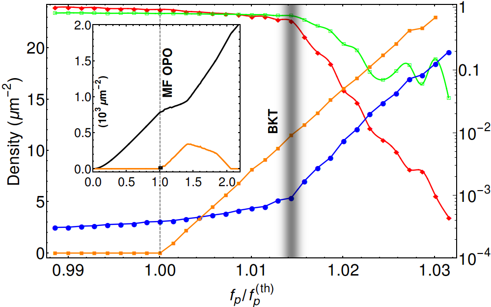
Figure 3: The phase diagram and the BKT transition. Inset: Mean-field photonic OPO densities for pump (black) $n_{p}$ and signal (orange) $n_{s}$ states as a function of increasing pump power $f_{p}$ rescaled by the threshold value $f_{p}^{\text{th}}$ (vertical black dashed line). The black square at $f_{p}\simeq f_{p}^{\text{th}}$ indicates the tiny pump strength interval close to mean-field threshold analysed in the main panel. Main panel: We plot with (orange) squares the same mean-field signal density $n_{s}$ as in the inset. All other data are noise averaged properties from stochastic simulations as a function of the pump strength. The noise averaged signal density $n_{s}$ is plotted with (blue) dots; the average vortex number in the signal rescaled by its average maximum value, $N_{\textrm{max}}=222.8$ with (red) diamonds; the noise averaged and symmetrised distance ratio $\langle b\rangle$ between nearest neighbouring V-V and AV-AV over V-AV pairs with (green) empty squares. The shaded region indicates the pump region for the BKT transition.

By evaluating other relevant noise averaged observable quantities, we are able to construct a phase diagram for the OPO transition in Fig. 3 and link it with the properties of the BKT transition. We evaluate the averaged signal photonic density at some time $t$ in the steady-state, $n_{s}=\int d{\mathbf{r}}\langle|\psi_{s}({\mathbf{r}},t)|^{2}\rangle/V$, where $V=(Na)^{2}$ is the system area and $\langle\dots\rangle$ indicates the noise average for the stochastic dynamics (blue dots). We also show the steady state signal density in the mean field (orange squares). The corresponding mean-field densities for both signal (orange line) and pump (black line) are presented for comparison in the inset of Fig. 3. At mean-field level, both signal and idler (not shown) suddenly switch on at the OPO threshold pump power, $f_{p}=f_{p}^{\text{th}}$ and both states are macroscopically occupied above threshold. The effect of fluctuations is to smoothen the sharp mean-field transition, as clearly shown by the (blue) dots in the main panel of Fig. 3, where we plot the noise average signal density $n_{s}$. This is because, even below the mean-field threshold, incoherent fluctuations weakly populate the signal. Note also that, even though somewhat smoothened, we can still appreciate a kink in the $n_{s}$ density, but at higher values of the pump power compared to the mean-field threshold $f_{p}^{\text{th}}$. We identify this as the novel BKT transition for our out-of-equilibrium system, as discussed more in detail below. This is further confirmed by a sudden decrease of the averaged number of vortices in the signal (red diamonds), and of the averaged distance between nearest neighbouring vortices of opposite winding number, $\langle b\rangle$ (green squares), as a function of the pump power concomitant with the observed kink for $n_{s}$. These results suggest that the system undergoes an OPO transition which, by including fluctuations above mean-field, is indeed analogous to the equilibrium BKT transition. Both vortices and antivortices proliferate below some threshold and, above, they bind to eventually disappear altogether. As indicated by the black square in the inset of Fig. 3, the region for such a crossover is indeed narrow in the pump strength.

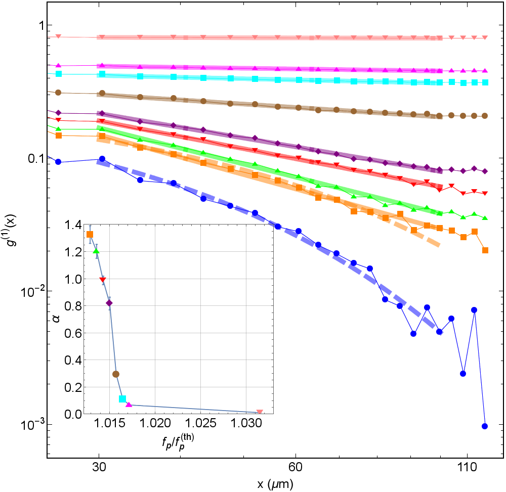
Figure 4: Algebraic and exponential decay of the first order correlation function across the BKT transition. Main panel: Long-range spatial dependence of $g^{(1)}({\mathbf{r}})$ for different pump powers $f_{p}/f_{p}^{\text{th}}$ close to the mean-field pump threshold (the symbols are the same ones as in the inset and correspond to the same values of $f_{p}/f_{p}^{\text{th}}$). Thick solid (thick dashed) lines are power-law (exponential) fitting, from which values of the exponent $\alpha$ are derived. The $f_{p}/f^{\textrm{th}}_{p}=1.0129$ case (orange squares) is a marginal case where both algebraic and exponential fits apply almost equally well, signalling the BKT transition region. Inset: Power-law algebraic decay exponent $\alpha$ for different pump powers $f_{p}/f_{p}^{\text{th}}$; error bars are standard deviations of the time-average.

First-order spatial correlations

For systems in thermal equilibrium, the BKT transition is associated with the onset of quasi-off-diagonal long-range order, i.e., with the algebraic decay of the first-order correlation function in the ordered phase, where vortices are bound, and exponential decay in the disordered phase, where free vortices do proliferate. In order to investigate whether the same physics applies to our out-of-equilibrium open-dissipative polariton system, we evaluate the signal first-order correlation function $g^{(1)}({\mathbf{r}})$ according to the prescription of Eq. (3) and characterise its long-range behaviour in Fig. 4. We observe the ordering transition as a crossover in the long-distance behaviour between an exponential decay in the disordered phase, $g^{(1)}({\mathbf{r}})\sim e^{-r/\xi}$, and an algebraic decay in the quasi-ordered phase, $g^{(1)}({\mathbf{r}})\sim(r/r_{0})^{-\alpha}$. We therefore fit the tail of the calculated correlation function to both of these functional forms and observe that, at the onset of vortex binding-unbinding and proliferation, the signal’s spatial correlation function changes its long-range nature, from exponential at lower pump powers to algebraic at higher (see Fig. 4).

However, in contrast with the thermal equilibrium case, we do observe that the exponent $\alpha$ of the power-law decay (inset of Fig. 4) can exceed the equilibrium upper bound of $1/4$ Nelson and Kosterlitz (1977), and can reach values as high as $\alpha\simeq 1.2$ for $f_{p}/f_{p}^{\text{th}}=1.0136$, just within the ordered phase. Further, as thoroughly discussed in Ref. SM , it is interesting to note that, close to the transition, we do observe a critical slowing down of the dynamics: Here, the convergence to a steady-state is dramatically slowed down compared to cases above or below the OPO transition, a common feature of other phase transitions. At the same time, close to threshold, the convergence of noise averaged number of vortices is much faster than the convergence of the power-law exponent $\alpha$. This indicates that the fluctuations induced by both the external drive and the decay preferentially excite collective excitations, rather than topological excitations, resulting in vortices being much more dynamically stable. Finally, note that for sufficiently strong pump powers, the power-law exponent becomes extremely small and thus quasi-long-range order is difficult to distinguish from the true long-range order over the entire system size.

Our findings explain why recent experimental studies, both in the OPO regime Spano et al. (2013), as well as for non-resonant pumping Roumpos et al. (2012), experienced noticeable difficulties in investigating the power-law decay of the first order correlation function across the transition. We do indeed find that the pump strength interval over which power-law decay can be clearly observed is extremely small, and the system quickly enters a regime where coherence extends over the entire system size, as measured in Spano et al. (2013). This was also observed in non-resonantly pumped experiments when using a single-mode laser Kasprzak et al. (2006). However, by intentionally adding extra fluctuations with a multimode laser pump, as in Roumpos et al. (2012), power-law decay was finally observed in the correlated regime, with an exponent in the range $\alpha\simeq 0.9-1.2$, in agreement with our results.

Discussion

Using microcavity polaritons in the optical parametric oscillator regime as the prototype of a driven-dissipative system, we have numerically shown that a mechanism analogous to the BKT transition, which governs the equilibrium continuous-symmetry-breaking phase transitions in two dimensions, occurs out of equilibrium for a driven-dissipative system of experimentally realistic size. Notwithstanding the novelty and significance of this result, there are a number of novel features which warrant discussion as they are peculiar to non-equilibrium phase transitions. We have observed that the exponent of algebraic decay in the quasi-long-range ordered phase exceeds what would be attainable in equilibrium. This recovers a recent observation Roumpos et al. (2012), and strongly suggests that indeed a non-equilibrium BKT may have been seen there. Moreover, our findings imply that the ordered phase is more robust to fluctuations induced by the external drive and decay than an analogous equilibrium ordered phase would be to thermal fluctuations. Although for realistic experimental conditions, we have found that the region for BKT physics, before the pump power is strong enough to induce perfect spatial coherence over the entire system size, is indeed narrow, we believe our work will encourage further experimental investigations in the direction of studying the non-equilibrium BKT phenomena. Even though the small size of the critical region has so far hindered its direct experimental study, our calculations indicate that the macroscopic coherence observed in past polariton experiments Keeling et al. (2007); Kasprzak et al. (2006); Stevenson et al. (2000); Baumberg et al. (2000); Carusotto and Ciuti (2013); Deng et al. (2010); Spano et al. (2013) results from a non-equilibrium phase transition of the BKT rather than the BEC kind.

Methods

We simulate the dynamics of the stochastic equations (2) with the XMDS2 software framework Dennis et al. (2012) using a fixed-step (where the fixed step-size ensures stochastic noise consistency) 4th order Runge-Kutta (RK) algorithm, which we have tested against fixed-step 9th order RK, and a semi-implicit fixed-step algorithm with 3 and 5 iterations. We choose the system parameters to be close to current experiments Sanvitto et al. (2010): The Rabi frequency is chosen as $\Omega_{R}=4.4$ meV, the mass of the microcavity photons is taken to be $m_{C}=2.3\times 10^{-5}m_{e}$, where $m_{e}$ is the electron mass, the mass of the excitons is much greater than this so we may take $m_{X}^{-1}\to 0$, the exciton and photon decay rates as $\kappa_{X}=\kappa_{C}=0.1$ meV, and the exciton-exciton interaction strength $g_{X}=0.002$ meV$\mu$m² Ferrier et al. (2011). The pump momentum ${\mathbf{k}}_{p}=(k_{p},0)$, with $k_{p}=1.6$ $\mu$m^-1, is fixed just above the inflection point of the LP dispersion, and its frequency, $\omega_{p}-\omega_{X}(0)=1.0$ meV, just below the bare LP dispersion. In order to satisfy the condition necessary to derive the truncated Wigner equation (2), $g_{X}/(\kappa_{X,C}dV)\ll 1$, whilst maintaining a sufficient spatial resolution and, at the same time, a large enough momentum range so that to resolve the idler state, simulations are performed on a 2D finite grid of $N\times N=280\times 280$ points and lattice spacing $a=0.866$ $\mu$m. Thus, the only system parameter left free to be varied is the pump strength $f_{p}$: We first solve the mean-field dynamics (1) in order to determine the pump threshold $f_{p}^{\text{th}}$ for the onset of OPO. We then vary the value of $f_{p}$ around $f_{p}^{\text{th}}$ in presence of the noise in order to investigate the nature of the OPO transition. We analyse the results from single noise realisations by filtering the full photonic emission for signal pump and idler, as described in the main text, as well as in SM . Further, we average all of our results over many independent realisations, which are either taken from $96$ independent stochastic paths or from multiple independent snapshots in time after the steady-state is reached: As thoroughly discussed in SM , 96 stochastic paths is shown to be sufficient to ensure the convergence of noise averaged observable quantities. For each noise realisation, vortices are counted by summing the phase difference (modulo $2\pi$) along each link around every elementary plaquette on the filtered grid. In the absence of a topological defect this sum is zero, while if the sum is $2\pi$ ($-2\pi$) we determine there to be a vortex (antivortex) at the center of the plaquette. The number of vortices is then averaged over the different stochastic paths or over time in the steady-state (see Ref. SM ): We consider the average number of vortices to be converged in time when its variation is less then $5\%$. Finally, the first order correlation function $g^{(1)}({\mathbf{r}})$ is evaluated according to Eq. (3), by averaging over both the noise and the auxiliary position ${\mathbf{R}}$; as discussed in SM , this can be computed efficiently in momentum space.

Acknowledgments
We thank J. Keeling for stimulating discussions. MHS acknowledges support from EPSRC (grants EP/I028900/2 and EP/K003623/2), FMM from the programs MINECO (MAT2011-22997) and CAM (S-2009/ESP-1503), and IC from ERC through the QGBE grant and from the Autonomous Province of Trento, partly through the project “On silicon chip quantum optics for quantum computing and secure communications” (“SiQuro”).

In this supplementary information we provide a more detailed account of some of the technical issues arising from our numerical methods, which are not of sufficiently general interest to warrant a discussion in the main text, but which are germane to the validity of our conclusions. In particular, we discuss the filtering we perform in order to isolate the signal state, and the loss in resolution this incurs, and we describe various tests we have undertaken in order to ensure that the results we present are properly converged.

I Momentum filtering

In order to study the condensate at the signal (or idler), we have to filter the full emission $\psi_{C}({\mathbf{r}},t)$ in such a way as to omit contributions with momentum outside a set radius about the signal (idler) states in $\mathbf{k}-$space. This applies both to the theory and the experimental data, and this procedure could equivalently be performed in either momentum or energy space. Here we filter in momentum space, and define:

$$\psi_{s,p,i}({\mathbf{r}},t)=\sum_{|{\mathbf{k}}-{\mathbf{k}}_{s,p,i}|<\tilde{k}_{s,p,i}}\psi_{C,{\mathbf{k}}}(t)e^{i{\mathbf{k}}\cdot{\mathbf{r}}},$$

where ${\mathbf{k}}_{s,p,i}$ is the momentum of the signal, pump and idler states respectively and $\tilde{k}_{s,p,i}$ is the filtering radius. We fix the filtering radius for the signal and idler to be $\tilde{k}_{s,i}=\tfrac{1}{2}|\mathbf{k}_{s,i}-\mathbf{k}_{p}|$ and choose to operate in the frame of reference co-moving with the signal (idler) so that the (physically irrelevant) background current does not show in the data. The filtering reveals the phase-freedom of the signal (idler) state at the expense of spatial resolution. Note, that this limits our ability to distinguish vortex-antivortex (V-AV) pairs with a separation less than a distance $\pi/\tilde{k}_{l}$, which for our chosen parameters is $\approx 2.708\mu\textrm{m}$. However, such extremely close vortex-antivortex pairs do not affect the spatial correlations of the field at large distances.

II Numerical Convergence

II.1 Number of stochastic realisations

The stochastic averages over the configurations of different realisations of the fields provide the expectation value of the corresponding symmetrically ordered operators. The realisation-averaged results presented in the main paper have been averaged over 96 realisations taken from independent stochastic paths as we assessed this to be sufficiently many to give a reliably converged result. In Fig. 1 we show the first order correlation function $g^{(1)}(x)$ for $f_{p}=1.017f_{p}^{\textrm{th}}$, averaged over different numbers of realisations (96, 192, 288, 384 and 480). We conclude that 96 is sufficient to determine the nature of the correlations.

The average number of vortices also does not change significantly (no more than $\pm 0.5$) beyond 96 realisations, and so we conclude that this number is sufficient to ensure consistent results in both the smooth and topological sectors of the model.

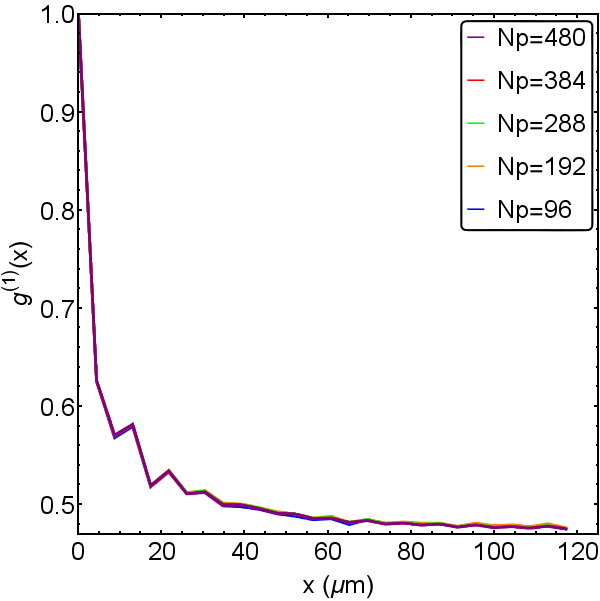
S. Fig. 1: Correlation function averaged over different numbers of realisations. The strength of the pump is fixed at $f_{p}=1.017f_{p}^{\textrm{th}}$, and each simulation is run well into the steady state. We calculate the correlation function averaged over 96, 192, 288, 384 and 480 realisations and observe no significant improvement in the convergence past 96 realisations.

II.2 Convergence in time to a steady state

In order to assess when a time evolution has reached its steady state we consider the average (over realisations) of both the signal density, $|\psi_{\textrm{s}}|^{2}$, and the number of vortices. In Figs. 2 and 3 we show the evolution of these quantities toward a steady state, assuming the initial condition wherein the system is allowed to reach its mean field steady state (at time $t=0$) and stochastic processes are adiabatically switched on. In practice this means that the noise terms are multiplied by a ramp function

$$r(t)=\frac{1}{2}\left[\tanh\left(\frac{t-t_{0}}{t_{r}}\right)+1\right]$$

such that the noise is slowly increases from $0$, achieving half its maximum at $t_{0}$, at a rate determined by $t_{r}$. For the empty cavity with noise initial condition, in which the pump is adiabatically increased, it is the pump term that is multiplied by this ramp function. We choose $t_{0}=450\textrm{ps}$ and $t_{r}=150\textrm{ps}$ as these prove to give a fairly rapid convergence to the steady state. It is, however, important to note that the steady state is unique and does not depend upon the specific values of $t_{0}$ and $t_{r}$ we choose nor on the initial conditions, which we start the dynamics from.

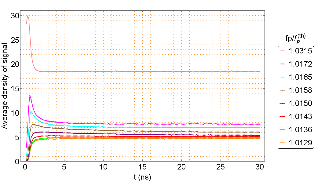
S. Fig. 2: Convergence in time of the average signal density. Here we show $|\psi_{\textrm{s}}|^{2}$ evolving in time for a range of pump powers. The initial jump in the signal occupation is induced by the introduction of stochastic processes, and dies away as the system resolves toward its non-equilibrium steady state.

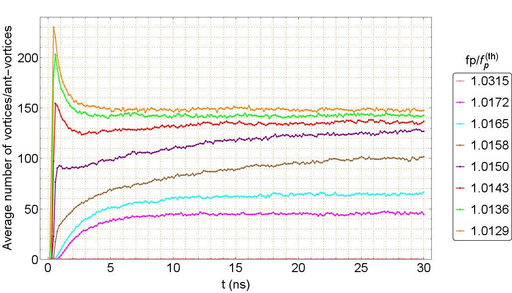
S. Fig. 3: Convergence in time of the average number of vortices. Here we show the average number of vortices in the system evolving in time for a range of pump powers. The introduction of stochastic processes increases the number of vortices (which is always zero in the spatially homogeneous mean field steady-state), which then evolves toward its steady state value through pair creation and annihilation events.

In all cases the steady state is reached within around twenty nanoseconds. The slowest convergence occurs in the vicinity of the BKT transition. This critical slowing of the dynamics is to be anticipated given the divergence of the correlation length as the transition is approached.

II.3 Realisations from independent stochastic paths vs. independent time snapshots in a single path

In Fig. 4 we show the number of vortices for a broad range of pump powers across the transition averaged over realisations taken from independent stochastic paths (red dots) and from multiple snapshots over time (blue dots) once the steady-state is reached. Averaging over time within the steady state is a less numerically intensive approach, and shows an excellent agreement with the average over realisations even in the critical region. In practice, averaging over time is computationally efficient away from the critical region, where the steady state is reached quickly and memory is quickly lost during the time evolution. Around the critical region it takes a significant time to reach a steady state and then to decorrelate the snapshots, so averaging over stochastic paths becomes more computationally effective.

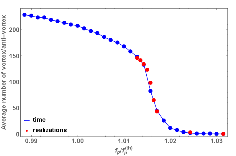
S. Fig. 4: Time versus stochastic realisations averaging. The red dots show number of vortices averaged over many stochastic paths. The blue dots show the number of vortices averaged over the final 500 frames, running from $15\textrm{ns}$ to $30\textrm{ns}$, of a single stochastic path, once the system has converged to a steady state. We observe an excellent agreement between these two approaches and so away from the critical region we can consider the (less numerically intensive) average over time.

II.4 Dependence on different initial conditions

We have investigated a number of physically diverse initial conditions in order to rule out dependence of the final steady state on the starting configuration. To initiate our simulations we either adiabatically increase the pump strength atop a white noise background or adiabatically increase the strength of the stochastic terms starting from the mean field steady state. We also wish to eliminate the possible effects of trapped vortices, and so in addition to simulations with a uniform pump region we have performed simulations, where a small strip around the numerical integration box is left un-pumped so as to act as a source/sink for vortices. The four distinct initial conditions we consider are therefore those classified in the following table:

	Increasing Pump	Increasing Noise
No Reservoir	Scheme A	Scheme B
Reservoir	Scheme D	Scheme C

In schemes A and D, there are initially very many vortices, which then proceed to annihilate with one another so that the overall vorticity tends to decrease toward the steady state. In schemes B and C there are no vortices at the outset but as stochastic processes shake the system the vorticity increases toward the steady state. Therefore even before the true steady state is reached, we can treat schemes A and D as upper bounds for the vorticity and schemes B and C as lower bounds. In schemes C and D we incorporate a reservoir (region with no drive and thus of very low density) of width $34.72\textrm{nm}$ along the two sides of the numerical integration box parallel to $k_{p}$, which we then exclude from calculations of the vorticity, signal density, and correlations. The width of the reservoir does not change the result except in that it needs to be wide enough that the condensate has room to decay away to zero.

In Supplementary Movie 1 we show the evolution towards the steady state for all four of these schemes with a pump power $f_{p}=1.017f_{p}^{\textrm{th}}$. We plot the vortex density (top panel) as well as dynamics of vortices (bottom panel, where blue and red dots show positions of V and AV cores) for each scheme (A, B, C and D starting from the left). We see that every scheme converges fairly rapidly towards the same steady state. From the animations it is evident that the vortices always appear in pairs but that these pairs are not always tightly bound. It was not a priori obvious that all four schemes should lead to the same steady state but we take this as evidence that the physical process leading to the steady state is universal for this system. We observe that the schemes incorporating an empty reservoir converge more quickly to the steady state than their counterparts without a reservoir. Nevertheless we present data for scheme B because the reservoirs have no counterpart in the traditional BKT transition to which we wish to compare our results.

III Fitting to the spatial correlation function

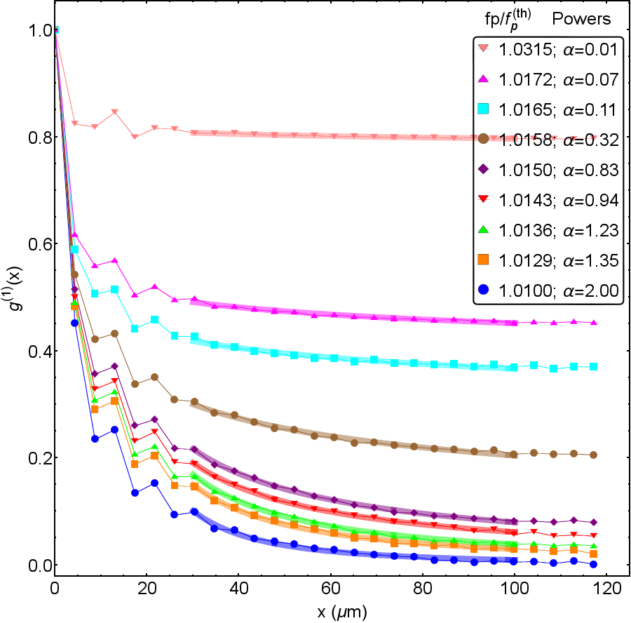
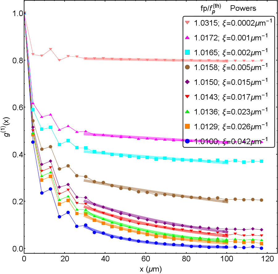
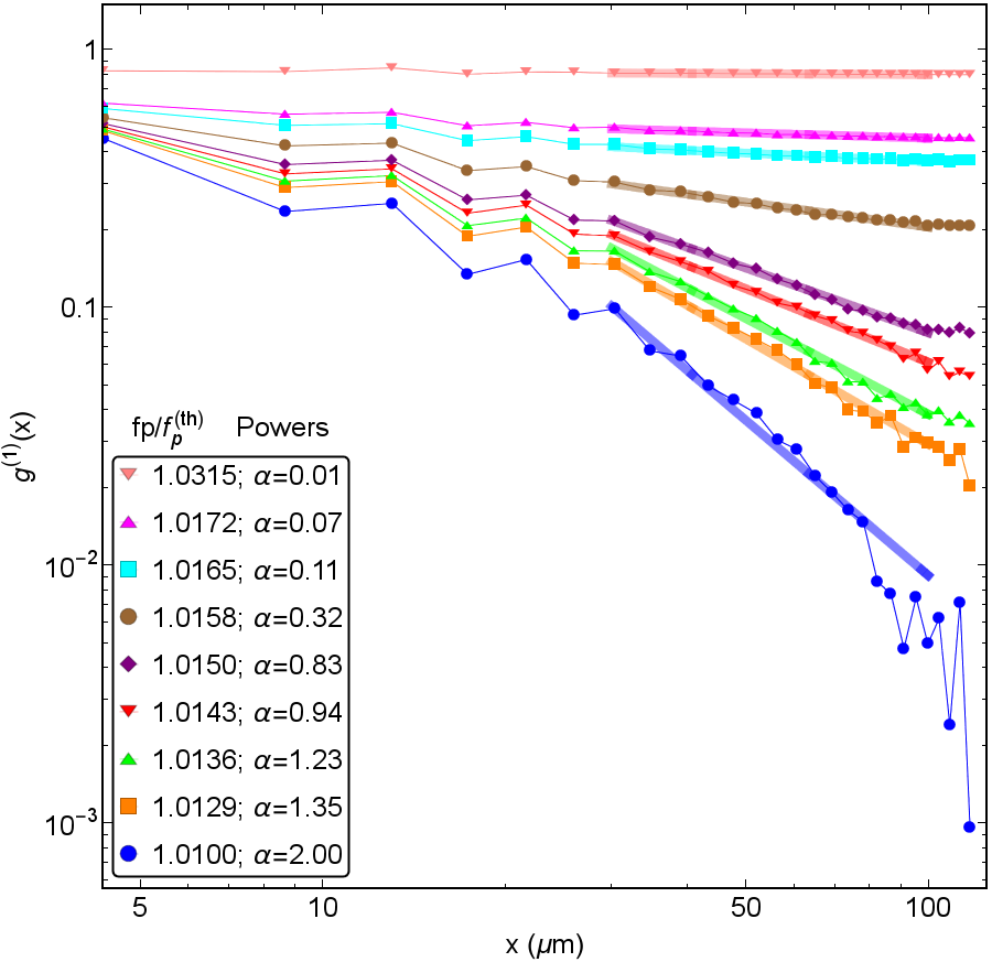
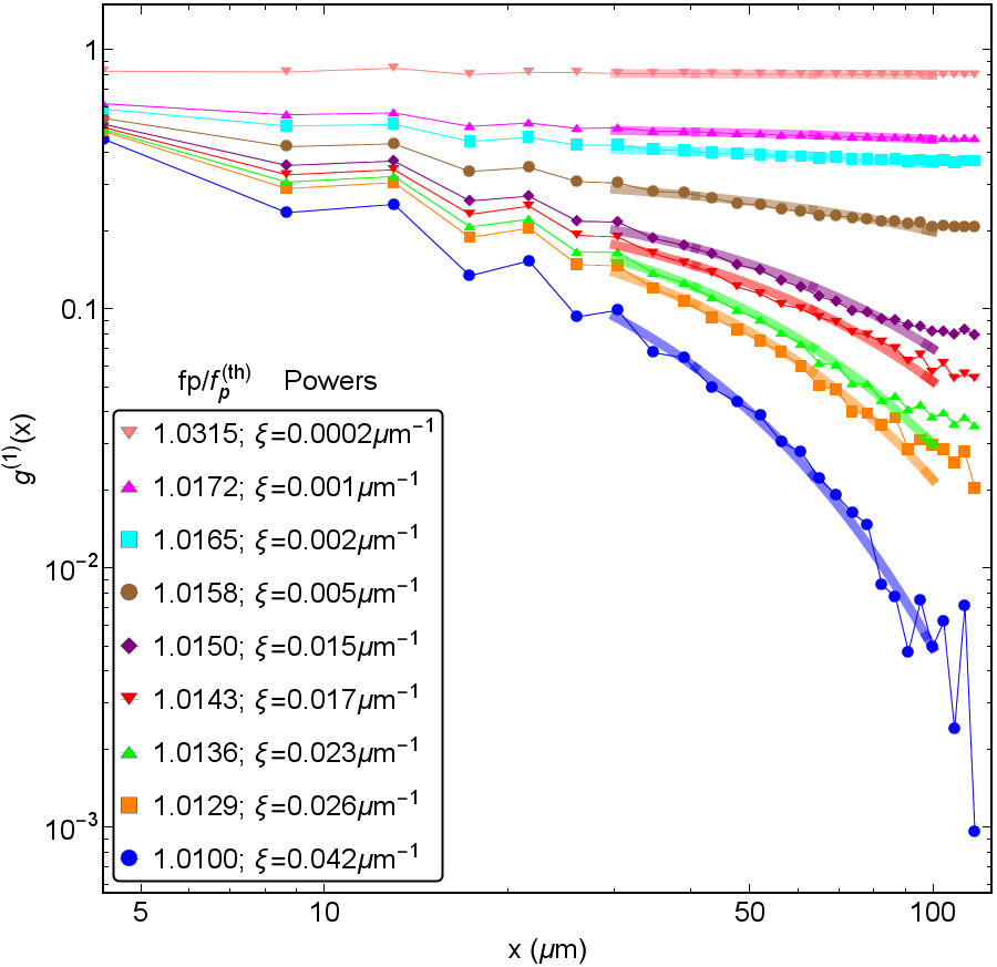
S. Fig. 5: Algebraic and exponential fits to the correlation function. Here we show both the algebraic (left) and exponential (right) fits to the correlation function on a full linear scale (above) and on an exponential scale (below). The fitting to the data is taken over the range $30\mu\textrm{m}<x<100\mu\textrm{m}$. This domain needs to avoid both the region close to origin with short-range correlations and the edges, where the behaviour might be influenced by periodic boundary conditions.

The behaviour of the first order correlation function $g^{(1)}(x)$, whether it decays as an exponential or as a power law, is determined by fitting the tail of the data to each functional form and taking the better fit of the two. The fitting is illustrated in Fig. 5. For pump powers close but above the critical region it is clear that the power-law fits the data better (which is also confirmed by a larger correlation coefficient), while below the critical region the exponential fit is closer to the data. For stronger pump powers, away from the transition, $g^{(1)}(x)$ is practically constant on these length-scales (as reported in experiments and discussed in the main text).

References

- Roumpos et al. (2012) G. Roumpos et al., Proc. Natl. Acad. Sci. U.S.A. 109, 6467 (2012).
- Mermin and Wagner (1966) N. Mermin and H. Wagner, Phys. Rev. Lett. 17, 1133 (1966).
- Chaikin and Lubensky (2000) P. M. Chaikin and T. C. Lubensky, Principles of condensed matter physics, vol. 1 (Cambridge Univ Press, 2000).
- Minnhagen (1987) P. Minnhagen, Rev. Mod. Phys. 59, 1001 (1987).
- Nelson and Kosterlitz (1977) D. Nelson and J. Kosterlitz, Phys. Rev. Lett. 39, 1201 (1977).
- Bishop and Reppy (1978) D. Bishop and J. Reppy, Phys. Rev. Lett. 40, 1727 (1978).
- Hadzibabic et al. (2006) Z. Hadzibabic, P. Krüger, M. Cheneau, B. Battelier, and J. Dalibard, Nature 441, 1118 (2006).
- Petrov et al. (2004) D. Petrov, D. Gangardt, and G. Shlyapnikov, J. Phys. IV 116, 5 (2004).
- Pitaevskii and Stringari (2003) L. Pitaevskii and S. Stringari, Bose-Einstein Condensation, International Series of Monographs on Physics (Clarendon Press, 2003).
- Carusotto and Ciuti (2013) I. Carusotto and C. Ciuti, Rev. Mod. Phys. (2013).
- Ritsch et al. (2013) H. Ritsch, P. Domokos, F. Brennecke, and T. Esslinger, Rev. of Mod. Phys. 85, 553 (2013).
- Carusotto et al. (2009) I. Carusotto et al., Phys. Rev. Lett. 103, 033601 (2009).
- Hartmann et al. (2008) M. J. Hartmann, F. G. S. L. Brandao, and M. B. Plenio, Laser Photon. Rev. 2, 527 (2008).
- Kasprzak et al. (2006) J. Kasprzak et al., Nature 443, 409 (2006).
- Deng et al. (2010) H. Deng, H. Haug, and Y. Yamamoto, Rev. Mod. Phys. 82, 1489 (2010).
- Amo et al. (2009a) A. Amo et al., Nature Phys. 5, 805 (2009a).
- Amo et al. (2009b) A. Amo et al., Nature 457, 291 (2009b).
- Sanvitto et al. (2010) D. Sanvitto et al., Nature Phys. 6, 527 (2010).
- Marchetti et al. (2010) F. Marchetti, M. H. Szymańska, C. Tejedor, and D. M. Whittaker, Phys. Rev. Lett. 105, 063902 (2010).
- Tosi et al. (2011) G. Tosi et al., Phys. Rev. Lett. 107, 036401 (2011).
- Roumpos and Yamamoto (2012) G. Roumpos and Y. Yamamoto, in Exciton Polaritons in Microcavities (Springer, 2012), pp. 85–146.
- Altman et al. (2013) E. Altman, L. M. Sieberer, L. Chen, S. Diehl, and J. Toner (2013), eprint arXiv:1311.0876.
- Stevenson et al. (2000) R. Stevenson et al., Phys. Rev. Lett. 85, 3680 (2000).
- Baumberg et al. (2000) J. Baumberg et al., Phys. Rev. B 62, R16247 (2000).
- Chiocchetta and Carusotto (2014) A. Chiocchetta and I. Carusotto, Phys. Rev. A 90, 023633 (2014).
- Vogel and Risken (1989) K. Vogel and H. Risken, Phys. Rev. A 39, 4675 (1989).
- Szymańska et al. (2007) M. H. Szymańska, J. Keeling, and P. B. Littlewood, Phys. Rev. B 75, 195331 (2007).
- Walls and Milburn (2007) D. F. Walls and G. J. Milburn, Quantum optics (Springer, 2007).
- Whittaker (2005) D. M. Whittaker, Phys. Rev. B 71, 115301 (2005).
- Wouters and Carusotto (2007a) M. Wouters and I. Carusotto, Phys. Rev. B 75, 075332 (2007a).
- Marchetti and Szymańska (2012) F. M. Marchetti and M. H. Szymańska, Vortices in polariton OPO superfluids (Springer-Verlag, 2012), vol. Springer Series in Solid-State Sciences, chap. Exciton Polaritons in Microcavities: New Frontiers.
- (32) See Supplemental Material for details on the model, used parameters, and numerical procedures.
- Wouters and Carusotto (2007b) M. Wouters and I. Carusotto, Phys. Rev. A 76, 043807 (2007b).
- Gardiner and Zoller (2004) C. Gardiner and P. Zoller, Quantum noise: a handbook of Markovian and non-Markovian quantum stochastic methods with applications to quantum optics, vol. 56 (Springer, 2004).
- Carusotto and Ciuti (2005) I. Carusotto and C. Ciuti, Phys. Rev. B 72, 1 (2005).
- Giorgetti et al. (2007) L. Giorgetti, I. Carusotto, and Y. Castin, Phys. Rev. A 76, 013613 (2007).
- Foster et al. (2010) C. J. Foster, P. Blakie, and M. J. Davis, Phys. Rev. A 81, 023623 (2010).
- Drummond and Walls (1980) P. Drummond and D. Walls, J. Phys. A 13, 725 (1980).
- Sieberer et al. (2013) L. M. Sieberer, S. D. Huber, E. Altman, and S. Diehl (2013), eprint arXiv:1309.7027v1.
- Spano et al. (2013) R. Spano et al., Opt. Express 21, 1 (2013).
- Keeling et al. (2007) J. Keeling, F. Marchetti, M. Szymańska, and P. Littlewood, Semicond. Sci. Technol. 22, R1 (2007).
- Dennis et al. (2012) G. R. Dennis, J. J. Hope, and M. T. Johnsson, Comput. Phys. Commun. 184, 201 (2012).
- Ferrier et al. (2011) L. Ferrier et al., Phys. Rev. Lett. 106, 126401 (2011).