From Markovian to non-Markovian persistence exponents

Abstract

We establish an exact formula relating the survival probability for certain Lévy flights (viz. asymmetric $\alpha$-stable processes where $\alpha=1/2$) with the survival probability for the order statistics of the running maxima of two independent Brownian particles. This formula allows us to show that the persistence exponent $\delta$ in the latter, non Markovian case is simply related to the persistence exponent $\theta$ in the former, Markovian case via: $\delta=\theta/2$.

Thus, our formula reveals a link between two recently explored families of anomalous exponents: one exhibiting continuous deviations from Sparre-Andersen universality in a Markovian context, and one describing the slow kinetics of the non Markovian process corresponding to the difference between two independent Brownian maxima.

I Introduction

In many applications of stochastic modeling, a key question regards the time that a random process will “survive” before reaching (or crossing, if the process has jumps) a certain point or absorbing boundary, away from which it started. Examples abound, from spin dynamics Baldassarri et al. (1999) to financial markets Majumdar and Bouchaud (2008), reaction kinetics Bénichou et al. (2010), biological systems Goel and Richter-Dyn (2004) or climate science Koscielny-Bunde et al. (1998), to name but a few Redner (2001).

Such survival times are usually described by the exponent governing the power-law decay of the long-time asymptotics for the first passage or first crossing time (FPT) density Baldassarri et al. (1999). They are linked with the time at which the maximum is achieved Knight (1996); Chaumont et al. (2001) and with excursions (fluctuations) away from the average Baldassarri et al. (2003). In a handful of cases, the probability density functions (pdf) associated with the FPT at $0$ can be computed exactly, e.g. for Brownian motion starting at $x_{0}>0$ with diffusion constant $D$, where the method of images yields the well-known density: $f_{D}(x_{0},\tau)=x_{0}(4\pi D\tau^{3})^{-1/2}\exp(-x_{0}^{2}/4D\tau)$, corresponding to a persistence exponent $\theta=1/2$.

As a consequence of E. Sparre Andersen’s celebrated theorem Sparre Andersen (1953, 1954), this value of $1/2$ expresses a universal behaviour that extends to the more general case of symmetric continuous time Markov processes Zumofen and Klafter (1995); Redner (2001); Chechkin et al. (2003); Koren et al. (2007a), even when the method of images breaks down Chechkin et al. (2003). In the case of skewed processes, however, the situation is more complex and offers a larger variety of exponents Koren et al. (2007b). De Mulatier et al de Mulatier et al. (2013) showed recently that the persistence exponent associated with the survival probability $P_{LF}^{(x_{0})}$ for asymmetric Lévy flights with stability index $\alpha\neq 1$ and asymmetry parameter $\beta\in[-1,1]$ can be computed exactly: the result is a family of exponents $\theta(\alpha,\beta)$, which continuously deviates from the Sparre Andersen value of $1/2$ (recovered for $\beta=0$).

In the case of non Markov processes, persistence exponents have been studied especially in connection with non-equilibrium dynamics and turbulence Merikoski et al. (2003); Oerding et al. (1997); Majumdar (1999); Paul and Schehr (2005); Henkel et al. (2011); Perlekar et al. (2011). Particular interest has been devoted to dynamical phenomena involving extreme-value processes Majumdar et al. (1996); Derrida et al. (1996); Sire (2007); Majumdar et al. (2010); Bray et al. (2013); Majumdar and Ziff (2008); Ben-Naim and Krapivsky (2014a). In a Letter published earlier this year (Ben-Naim and Krapivsky, 2014b), Ben-Naim and Krapivsky computed the persistence exponent associated with the order statistics of two Brownian maxima (see Fig. 1). They showed that if $m_{1}-m_{2}=a>0$ initially, the probability $P_{BM}^{(a)}(t)$ that the maxima have remained ordered in the same way up to a time $\tau$, decays, when $\tau$ is large, like $\tau^{-\delta}$, where $\delta$ is linked to the diffusion constants of the Brownian particles as follows: $\delta(D_{1},D_{2})=(1/\pi)\arctan(\sqrt{D_{2}/D_{1}})$. In particular, when $D_{1}=D_{2}$, $\delta=1/4$.

In this paper, we establish a formula that relates the survival probability of certain Lévy flights (therefore Markov processes) studied by de Mulatier et al., with the survival probability examined by Ben-Naim and Krapivsky in a non Markovian context:

$$P_{BM}^{(a)}(t) = 2\,\int_{a}^{\infty}dm\ p_{D_{1}}(a,m;t)\,\times\int_{0}^{\infty}ds\ f_{D_{2}}(a,s)\,P_{LF}^{(s)}(m).$$ (1)

($f_{D}$ is the FPT density for Brownian motion, and $p_{D}$ is the standard Brownian propagator.)

This formula allows us to show how the persistence exponents in both cases are directly related via:

$$\delta(D_{1},D_{2})=\theta(\alpha,\beta)/2,$$ (2)

with $\alpha=1/2$ and $\beta=\left(\sqrt{D_{1}}-\sqrt{D_{2}}\right)/\left(\sqrt{D_{1}}+\sqrt{D_{2}}\right)$. Thus, our formula also reveals how the $1/4$-exponent obtained in (Ben-Naim and Krapivsky, 2014b) when $D_{1}=D_{2}$, can be derived directly from the Sparre-Andersen universal behaviour of an underlying, hidden Markov process governing the order statistics of the two Brownian maxima.

A key point on which we base our reasoning is the fact, noted by P. Lévy Lévy (1948), that the path of the running-maximum process, $M(t)$, of a Brownian motion, is strictly increasing and therefore admits a reciprocal function. This function corresponds to the path of a process, $T(x)$, which is also strictly increasing. But contrary to $M(t)$, $T(x)$ is Markovian. We shall first recall some details about the $T$ process and about general Lévy-Brownian processes, before establishing our results.

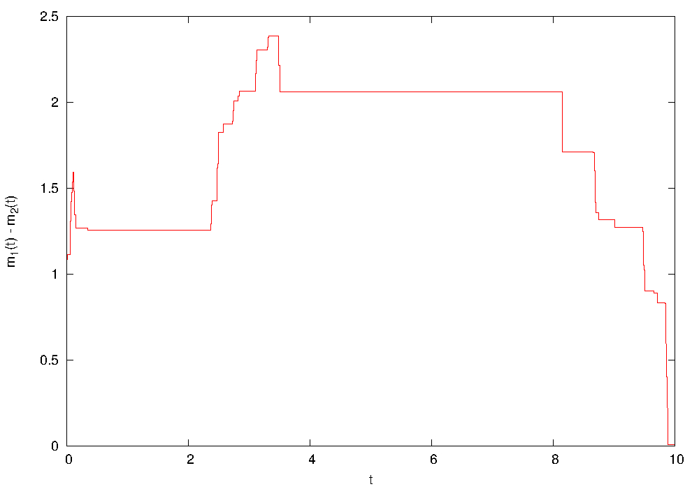
Figure 1: Sample path, until it first crosses $0$, of the non Markov process $m_{1}(t)-m_{2}(t)$, where $m_{1}$ and $m_{2}$ are the running maxima of two independent Brownian walkers.

II Hitting times of new maxima

Consider a Brownian motion on the real line, with diffusion constant $D$ and with position at time $t$ given by $B(t)$. The transition probability for the motion, sometimes called the free particle propagator, is the well known Gaussian kernel $p_{D}(x,y;\tau)=(4\pi D\tau)^{-\frac{1}{2}}\exp\left\{-(y-x)^{2}/4D\tau\right\}$, which gives the probability density to find the particle in $y$ at time $t+\tau$ given that it was in $x$ at time $t$.

From $B$, the maximum process, that corresponds to the running maximum of the Brownian motion at time $t$, is defined as $M(t)=\mathrm{max}\left\{B(\tau),0\leq\tau\leq t\right\}$. Using for instance the method of images, one easily shows that the pdf for $M(t)$ is just twice the pdf for $B(t)$, that is $2\,p_{D}(x_{0},M;t)$.

One of the difficulties when working with Brownian maxima is the fact that $M$ is not a Markov process. In some cases, this difficulty can be circumvented by working with $M(t)-B(t)$ which is Markovian (and actually happens to be simply a reflected Brownian motion). In other cases, it can prove useful to rely on a perhaps lesser-known process, associated with the times when new maxima are achieved: $T(x)=\inf\left\{t\geq 0,B(t)=x\right\}$.

Lévy showed that $T$ is Markovian and $\alpha$-stable with $\alpha=1/2$, since the characteristic function (which is just the Fourier transform of the law) of the random variable $T(x)$ has the form Lévy (1948):

$$\mathbb{E}\left[e^{iuT(x)}\right]=e^{-(1-i\ \mathrm{sign}(u))x\sqrt{\frac{\mid u\mid}{2D}}},$$ (3)

where $\mathbb{E}\left[\dots\right]$ denotes probabilistic expectation, and $\mathrm{sign}(u)$ is the sign of $u$. When the diffusion constant $D$ is $1/2$, this process is called the standard stable subordinator of index $1/2$. Its propagator can be expressed easily Mörters and Peres (2010) from the first-passage time density of Brownian motion, and one finds a transition kernel from $s$ to $t>s$ in a “time” $a$ given by:

$$f_{D}(a,t-s)=\frac{a}{\sqrt{4\pi D(t-s)^{3}}}e^{-\frac{a^{2}}{4D(t-s)}}.$$ (4)

(Recall that here $a$ is the time parameter for the $T$ process, while $s$ and $t$ correspond to positions. Also, note that this is a densitiy in $t$ and therefore will be multiplied by $dt$ upon integration so that, dimension-wise, there is nothing wrong with the denominator.)

Stable subordinators are an extreme case of $\alpha$-stable processes. These processes play an important role in line with the generalized central limit theorem Feller (1968): so-called Lévy flights, also known as Lévy-Brownian motions Dybiec et al. (2006), have emerged as powerful tools to model non Gaussian phenomena Parashar et al. (2008); Zeng and Xu (2010); Penland and Ewald (2008); Janakiraman and Sebastian (2014); Risau-Gusman et al. (2013). They are continuous time Markov processes that can be described in Langevin formalism as generalized Brownian motion, where the driving term, instead of a simple Gaussian white noise is a general Lévy noise $\zeta$, that induces independent increments identically distributed according to an $\alpha$-stable law Dybiec et al. (2006): $\dot{x}(t)=\zeta(t)$. Such stable laws are specified by four parameters Applebaum (2009): their stability index $\alpha\in]0,2]$, a scale parameter $\sigma$, a location parameter $\mu$, and a skewness parameter $\beta$. For $\alpha\neq 1$, the characteristic function of their position at time $t$ admits the following Lévy-Khintchine general form Koren et al. (2007a):

$$\phi_{t}(u)=e^{i\mu u-\sigma^{\alpha}t\mid u\mid^{\alpha}\left(1-i\beta\tan\left(\frac{\pi}{2}\alpha\right)\mathrm{sign}(u)\right)}.$$ (5)

Standard Brownian motion corresponds to $\alpha=2$, the Cauchy-Lorentz process is $\alpha=1,\beta=0$, and the Lévy-Smirnov driven process, with $\alpha=0.5,\beta=1$, is the same as the stable subordinator mentioned above.

III Time-lag process

Let now $B_{1}$ and $B_{2}$ be two independent Brownian walkers. Write $m_{1}$ and $m_{2}$ for their running maxima and write $T_{1}$ and $T_{2}$ for the associated hitting-time processes as defined in the previous section. We set $Z(x)=T_{2}(x)-T_{1}(x)$ and call $Z$ the time-lag process: indeed, if $Z(x)=\tau$, it means that, compared to $B_{1}$, $B_{2}$ first hit $x$ with a delay $\tau$.

The important point here is that if $m_{1}$ and $m_{2}$ switch order, so will $T_{1}$ and $T_{2}$, and therefore $Z$ will change signs. One can therefore compute the probability that $m_{1}$ and $m_{2}$ remain in the same order up to time $t$ by examining the probability that $Z$ remains positive on the interval $\left[0,m_{1}(t)\right]$ (of course, one will need to pay attention to the fact that the right-hand side of this interval is itself a random variable).

Let us first determine the characteristic function of $Z(x)$, in terms of the diffusion constants $D_{1}$ and $D_{2}$. Using the independence of $T_{1}$ and $T_{2}$, one has:

$$\mathbb{E}\left[e^{iuZ(x)}\right]=\mathbb{E}\left[e^{iuT_{2}(x)}\right]\mathbb{E}\left[e^{-iuT_{1}(x)}\right].$$ (6)

Substituting formula (3) for the characteristic functions on the right-hand side yields:

$$\mathbb{E}\left[e^{iuZ(x)}\right] = \exp\left\{-\left(1-i\frac{\sqrt{D_{1}}-\sqrt{D_{2}}}{\sqrt{D_{1}}+\sqrt{D_{2}}}\ \mathrm{sign}(u)\right)\ \left(\frac{\sqrt{D_{1}}+\sqrt{D_{2}}}{\sqrt{2D_{1}D_{2}}}\right)x\sqrt{\mid u\mid}\right\}.$$ (7)

From this characteristic function and (5), one can readily identify an $\alpha$-stable process with $\alpha=1/2$, and asymmetry coefficient $\beta=\left(\sqrt{D_{1}}-\sqrt{D_{2}}\right)/\left(\sqrt{D_{1}}+\sqrt{D_{2}}\right)$. We immediately notice that when the diffusion constants are the same, $\beta$ will be zero and therefore $Z$ will simply be a symmetric Lévy flight. We will make use of this observation in section 5, but let us first derive a general formula.

IV General formula

Let $B_{1}$ and $B_{2}$ have diffusion constants $D_{1}$ and $D_{2}$, and let $B_{1}(0)=a$ with $a>0$, and $B_{2}(0)=0$. In this case, $T_{1}(x)$ is not defined for $x<a$, but $T_{1}(a)=0$. Also $T_{2}(0)=0$ and $T_{2}(a)$ is distributed according to the transition kernel (4) — so it has almost surely some strictly positive value. Hence, $Z(x)=T_{2}(a+x)-T_{1}(a+x)$ is a $1/2$-stable Lévy flight that starts at some value $T_{2}(a)>0$.

Now we wish to encode the fact that the time-lag process does not have any zero crossing before “time” $m_{1}(t)$ (recall that the time space for the $Z$ process is the position space for the Brownian particles). This is saying that the first time at which $Z$ crosses $0$ should be larger than $m_{1}(t)$ and it can be expressed in terms of the survival probability $P_{LF}\left(m_{1}(t)\right)$, provided that the initial value, $T_{2}(a)$, is averaged out using $f_{D_{2}}(a,s)$, the propagator from (4):

$$R(m_{1},a)=\int_{0}^{\infty}ds\ f_{D_{2}}(a,s)\,P_{LF}^{(s)}(m_{1}(t)).$$ (8)

We can now write our general formula for $P_{BM}(t)$ by integrating (8) over $m_{1}(t)$:

$$P_{BM}^{(a)}(t)=\int_{a}^{\infty}dm\ 2\,p_{D_{1}}(a,m;t)\,R(m,a).$$ (9)

Of course, $P_{BM}(t)$ depends on $a$, the initial distance between the two walkers. Also, to compute $P_{BM}(t)$ more explicitly, one would need to know the exact form of $\rho_{s}(x)$, the pdf for the time at which a $1/2$-stable Lévy flight with characteristic function as in (7) first crosses $0$, having started at $s$. This would allow the computation of $P_{LF}^{(s)}$. Unfortunately, such pdfs are known explicitly only for very few Lévy processes: as soon as jumps are not negligible (as is the case for $1/2$-stable processes), hitting times and crossing times differ, and standard methods like the method of images fail Chechkin et al. (2003); Koren et al. (2007a). However, one can extract from (9) a non-trivial relationship between some Markovian persistence exponents and some non Markovian ones, as we shall now see.

V Bijection between exponents

In the general case, when the diffusion constants are different, the time-lag process $Z$ will be $1/2$-stable but asymmetric, with a skewness coefficient $\beta=\left(\sqrt{D_{1}}-\sqrt{D_{2}}\right)/\left(\sqrt{D_{1}}+\sqrt{D_{2}}\right)$. Such asymmetric Lévy flights are found to have power-law tailed persistence de Mulatier et al. (2013), so that if one writes $\theta(1/2,\beta)$ (or simply $\theta$ here) for their persistence exponents, one can express in terms of these the exponent governing the asymptotics of $P_{BM}(t)$. Indeed, from (8) and (9):

$$P_{BM}(t)=\int_{a}^{\infty}dm\ 2\,p_{D_{1}}(a,m;t)\ \int_{0}^{\infty}ds\ f_{D_{2}}(a,s)\,\int_{m}^{\infty}dx\ \rho_{s}(x)$$

$$= \int_{0}^{\infty}ds\ f_{D_{2}}(a,s)\,\int_{0}^{\infty}dx\ \rho_{s}(x+a)\ \mathrm{erf}\left(\frac{x}{\sqrt{2t}}\right)$$

$$= \sqrt{2t}\int_{0}^{\infty}ds\ f_{D_{2}}(a,s)\ \int_{0}^{\infty}dx\ \rho_{s}(x\sqrt{2t}+a)\ \mathrm{erf}\left(x\right).$$

And, using $\rho_{s}(v)\sim h(s)\,v^{-(1+\theta)}$ when $v$ is large, with $h$ a function of the initial point $s$, one finds that:

$$P_{BM}(t)\sim\sqrt{2t}\int_{0}^{\infty}ds\ f_{D_{2}}(a,s)\ \int_{0}^{\infty}dx\ h(s)\ (x\sqrt{2t}+a)^{-(1+\theta)}\ \mathrm{erf}\left(x\right)$$ (10)

$$\sim (\sqrt{2t})^{-\theta}\int_{0}^{\infty}ds\ h(s)\ f_{D_{2}}(a,s)\,\int_{0}^{\infty}dx\ x^{-(1+\theta)}\ \mathrm{erf}\left(x\right)$$

$$\sim \ \tilde{h}(a)\ t^{-\frac{\theta}{2}}.$$

(We have used the fact that any finite $a>0$ will become negligible compared to $\sqrt{2t}$ when $t$ becomes large enough, and we write $\tilde{h}$ for the function obtained from the remaining integrals.)

Thus, we obtain our second main result:

$$P_{BM}(t)\sim t^{-{\theta(\beta)/2}}.$$ (11)

To confirm this result, note that we know from de Mulatier et al. (2013) the exact value of $\theta(\beta)$: this is given by $1/2-2/\pi\arctan(\beta)$. It is then easy to see, by means of a simple trigonometric identity, that with $\beta$ as stated in (7) in terms of $D_{1}$ and $D_{2}$, one finds: $\theta(\beta)/2=(1/\pi)\arctan\left(\sqrt{D_{2}/D_{1}}\right)$, in full agreement with Ben-Naim and Krapivsky (2014b).

Also, in simple, extreme cases, one recovers intuitive results: eg for $D_{1}\gg D_{2}$, one expects $P(t)$ to be equal to $1$ as the running maximum of the first particle will keep being too high for the second particle to exceed it. In this case, $\beta\rightarrow 1$ and one sees from formula (7) that the time-lag process reduces to a $1/2$-stable subordinator, that is a jump process with purely positive jumps, so that $Z$ never crosses $0$ and $P(t)=1$ indeed.

VI Hidden Sparre Andersen behaviour

An interesting phenomenon is to be noticed in the special case when the two Brownian motions have the same diffusion constant. Then, $\beta=0$ and the time-lag process becomes symmetric. Therefore, the pdf for its first crossing time will obey the universal Sparre Andersen behaviour so that $\rho_{s}(x)\sim h(s)x^{-3/2}$, and equivalently $\theta(\beta)=1/2$. Our second main result, Equation (11), therefore sheds light on how the anomalous $1/4$-exponent computed in Ben-Naim and Krapivsky (2014b) emerges from the underlying “standard” Sparre Andersen behaviour of the time-lag process.

VII Conclusion

We have established an exact formula for the survival probability $P_{BM}(t)$ of the order of two Brownian maxima, by linking it with the survival probability of an underlying Lévy flight. This yields a bijection between non trivial persistence exponents. Via the results in (Ben-Naim and Krapivsky, 2014b), our formula also establishes a link between persistence exponents for asymmetric $1/2$-stable Lévy flights and an eigenvalue of the angular component of the 2-dimensional Laplace operator.

One of the main features of the method used in this paper is the fact that it maps a non Markov problem onto a Markov one, moving from Brownian maxima to Lévy flights. The extent to which the same mapping may be used to obtain other results, in this and other contexts (order statistics of more than two maxima, higher dimension,…), should and will be investigated.

References

- Baldassarri et al. (1999) A. Baldassarri, J. P. Bouchaud, I. Dornic, and C. Godrèche, Phys. Rev. E 59, R20 (1999).
- Majumdar and Bouchaud (2008) S. N. Majumdar and J.-P. Bouchaud, Quantitative Finance 8, 753 (2008), http://dx.doi.org/10.1080/14697680802569093 .
- Bénichou et al. (2010) O. Bénichou, C. Chevalier, J. Klafter, B. Meyer, and R. Voituriez, Nature chemistry 2, 472 (2010).
- Goel and Richter-Dyn (2004) N. Goel and N. Richter-Dyn, Stochastic Models in Biology (Blackburn Press, 2004).
- Koscielny-Bunde et al. (1998) E. Koscielny-Bunde, A. Bunde, S. Havlin, H. Roman, Y. Goldreich, and H.-J. Schellnhuber, Phys. Rev. Lett. 81, 729 (1998).
- Redner (2001) S. Redner, A Guide to First-Passage Processes (Cambridge University Press, 2001).
- Knight (1996) F. Knight, Astérisque 236, 171 (1996).
- Chaumont et al. (2001) L. Chaumont, D. Holson, and M. Yor, in Séminaire de Probabilités XXXV, Lecture Notes in Mathematics, Vol. 1755, edited by J. Azéma, M. Émery, M. Ledoux, and M. Yor (Springer Berlin Heidelberg, 2001) pp. 334–347.
- Baldassarri et al. (2003) A. Baldassarri, F. Colaiori, and C. Castellano, Phys. Rev. Lett. 90, 060601 (2003).
- Sparre Andersen (1953) E. Sparre Andersen, Mathematica Scandinavica 1, 263 (1953).
- Sparre Andersen (1954) E. Sparre Andersen, Mathematica Scandinavica 2, 195 (1954).
- Zumofen and Klafter (1995) G. Zumofen and J. Klafter, Phys. Rev. E 51, 2805 (1995).
- Chechkin et al. (2003) A. V. Chechkin, R. Metzler, V. Y. Gonchar, J. Klafter, and L. V. Tanatarov, Journal of Physics A: Mathematical and General 36, L537 (2003).
- Koren et al. (2007a) T. Koren, A. Chechkin, and J. Klafter, Physica A: Statistical Mechanics and its Applications 379, 10 (2007a).
- Koren et al. (2007b) T. Koren, M. Lomholt, A. Chechkin, J. Klafter, and R. Metzler, Phys. Rev. Lett. 99, 160602 (2007b).
- de Mulatier et al. (2013) C. de Mulatier, A. Rosso, and G. Schehr, Journal of Statistical Mechanics: Theory and Experiment 2013, P10006 (2013).
- Merikoski et al. (2003) J. Merikoski, J. Maunuksela, M. Myllys, J. Timonen, and M. Alava, Phys. Rev. Lett. 90, 024501 (2003).
- Oerding et al. (1997) K. Oerding, S. Cornell, and A. Bray, Phys. Rev. E 56, R25 (1997).
- Majumdar (1999) S. N. Majumdar, Current Science 77, 370 (1999).
- Paul and Schehr (2005) R. Paul and G. Schehr, EPL (Europhysics Letters) 72, 719 (2005).
- Henkel et al. (2011) M. Henkel, H. Hinrichsen, M. Pleimling, and S. Lübeck, Non-Equilibrium Phase Transitions: Volume 2: Ageing and Dynamical Scaling Far from Equilibrium, Theoretical and Mathematical Physics (Springer, 2011).
- Perlekar et al. (2011) P. Perlekar, S. Ray, D. Mitra, and R. Pandit, Phys. Rev. Lett. 106, 054501 (2011).
- Majumdar et al. (1996) S. Majumdar, C. Sire, A. Bray, and S. Cornell, Phys. Rev. Lett. 77, 2867 (1996).
- Derrida et al. (1996) B. Derrida, V. Hakim, and R. Zeitak, Phys. Rev. Lett. 77, 2871 (1996).
- Sire (2007) C. Sire, Phys. Rev. Lett. 98, 020601 (2007).
- Majumdar et al. (2010) S. Majumdar, A. Rosso, and A. Zoia, Phys. Rev. Lett. 104, 020602 (2010).
- Bray et al. (2013) A. J. Bray, S. N. Majumdar, and G. Schehr, Advances in Physics 62, 225 (2013), http://dx.doi.org/10.1080/00018732.2013.803819 .
- Majumdar and Ziff (2008) S. Majumdar and R. Ziff, Phys. Rev. Lett. 101, 050601 (2008).
- Ben-Naim and Krapivsky (2014a) E. Ben-Naim and P. L. Krapivsky, Journal of Physics A: Mathematical and Theoretical 47, 255002 (2014a).
- Ben-Naim and Krapivsky (2014b) E. Ben-Naim and P. L. Krapivsky, Phys. Rev. Lett. 113, 030604 (2014b).
- Lévy (1948) P. Lévy, Processus stochastiques et mouvement brownien (Gauthiers-Villars, Paris, 1948).
- Mörters and Peres (2010) P. Mörters and Y. Peres, Brownian Motion, Cambridge Series in Statistical and Probabilistic Mathematics (Cambridge University Press, 2010).
- Feller (1968) W. Feller, An Introduction to Probability Theory and its Applications (Wiley, New York, 1968).
- Dybiec et al. (2006) B. Dybiec, E. Gudowska-Nowak, and P. Hänggi, Phys. Rev. E 73, 046104 (2006).
- Parashar et al. (2008) R. Parashar, D. O’Malley, and J. Cushman, Phys. Rev. E 78, 052101 (2008).
- Zeng and Xu (2010) L. Zeng and B. Xu, Physica A: Statistical Mechanics and its Applications 389, 5128 (2010).
- Penland and Ewald (2008) C. Penland and B. D. Ewald, Philosophical Transactions of the Royal Society of London A: Mathematical, Physical and Engineering Sciences 366, 2455 (2008).
- Janakiraman and Sebastian (2014) D. Janakiraman and K. L. Sebastian, Phys. Rev. E 90, 040101 (2014).
- Risau-Gusman et al. (2013) S. Risau-Gusman, S. Ibáñez, and S. Bouzat, Phys. Rev. E 87, 022105 (2013).
- Applebaum (2009) D. Applebaum, Lévy processes and stochastic calculus (Cambridge university press, 2009).