The Smaller (SALI) and the Generalized (GALI) Alignment Indices: Efficient Methods of Chaos Detection

Abstract

We provide a concise presentation of the Smaller (SALI) and the Generalized Alignment Index (GALI) methods of chaos detection. These are efficient chaos indicators based on the evolution of two or more, initially distinct, deviation vectors from the studied orbit. After explaining the motivation behind the introduction of these indices, we sum up the behaviors they exhibit for regular and chaotic motion, as well as for stable and unstable periodic orbits, focusing mainly on finite-dimensional conservative systems: autonomous Hamiltonian models and symplectic maps. We emphasize the advantages of these methods in studying the global dynamics of a system, as well as their ability to identify regular motion on low dimensional tori. Finally we discuss several applications of these indices to problems originating from different scientific fields like celestial mechanics, galactic dynamics, accelerator physics and condensed matter physics.

1 Introduction and Basic Concepts

A fundamental aspect in studies of dynamical systems is the identification of chaotic behavior, both locally, i.e. in the neighborhood of individual orbits, and globally, i.e. for large samples of initial conditions. The most commonly used method to characterize chaos is the computation of the maximum Lyapunov exponent (mLE) $\lambda_{1}$. In general, Lyapunov exponents (LEs) are asymptotic measures characterizing the average rate of growth or shrinking of small perturbations to orbits of dynamical systems. They were introduced by Lyapunov Lyapunov_1892 and they were applied to characterize chaotic motion by Oseledec in O_68 , where the Multiplicative Ergodic Theorem (which provided the theoretical basis for the numerical computation of the LEs) was stated and proved. For a recent review of the theory and the numerical evaluation of LEs the reader is referred to S_10 . The numerical evaluation of the mLE was achieved in the late 1970’s BGS_76 ; NS_77 ; CGG_78 and allowed the discrimination between regular and chaotic motion. This evaluation is performed through the time evolution of an infinitesimal perturbation of the orbit’s initial condition, which is described by a deviation vector from the orbit itself. The evolution of the deviation vector is governed by the so-called variational equations CGG_78 .

In practice, $\lambda_{1}$ is evaluated as the limit for $t\rightarrow\infty$ of the finite time maximum Lyapunov exponent

$$\Lambda_{1}(t)=\frac{1}{t}\ln\frac{\|\vec{w}(t)\|}{\|\vec{w}(0)\|},$$ (1)

where $t$ denotes the time and $\|\vec{w}(0)\|$, $\|\vec{w}(t)\|$ are the Euclidean norms of the deviation vector $\vec{w}$ at times $t=0$ and $t>0$ respectively. Thus

$$\lambda_{1}=\lim_{t\rightarrow\infty}\Lambda_{1}(t).$$ (2)

The computation of the mLE was extensively used for studying chaos and it is still implemented nowadays for this purpose. Nevertheless, one of its major practical disadvantages is the slow convergence of the finite time Lyapunov exponent (1) to its limit value (2). Since $\Lambda_{1}(t)$ is influenced by the whole evolution of the deviation vector, the time needed for it to converge to $\lambda_{1}$ is not known a priori, and in many cases it may become extremely long. This delay can result in CPU-time expensive computations, especially when the study of many orbits is required for the global investigation of a system. In order to overcome this problem several other fast chaos detection techniques have been developed over the years; some of which are presented in this volume.

Throughout this chapter we consider finite-dimensional conservative dynamical systems and in particular, autonomous Hamiltonian models and symplectic maps (except from Sect. 4.3 where a time dependent Hamiltonian system is studied). In these systems regular motion occurs on the surface of a torus in the system’s phase space and is characterized by $\lambda_{1}=0$. Any deviation vector $\vec{w}(0)$ from a regular orbit eventually falls on the tangent space of this torus and its norm will approximately grow linearly in time, i.e. eventually becoming proportional to $t$, $\|\vec{w}(t)\|\propto t$. Consequently, $\Lambda_{1}(t)\propto\ln t/t$, which practically means that $\Lambda_{1}(t)$ tends asymptotically to zero following the power law $t^{-1}$ because the values of $\ln t$ change much slower than $t$ as time grows (see for example BGS_76 ; CCF_80 and Sect. 5.3 of S_10 ). On the other hand, in the case of chaotic orbits the use of any initial deviation vector in (1) and (2) practically leads to the computation of the mLE $\lambda_{1}>0$ because this vector eventually is stretched towards the direction associated to the mLE, assuming of course that $\lambda_{1}>\lambda_{2}$, with $\lambda_{2}$ being the second largest LE. We note here that, from the first numerical attempts to evaluate the mLE BGS_76 ; CGG_78 it became apparent that a random choice of the initial deviation vector $\vec{w}(0)$ leads with probability one to the computation of $\lambda_{1}$. This means that, the choice of $\vec{w}(0)$ does not affect the limiting value of $\Lambda_{1}(t)$, but only the initial phases of its evolution. This behavior introduces some difficulties when we want to evaluate the whole spectrum of LEs of chaotic orbits because any set of initially distinct deviation vectors eventually end up to vectors aligned along the direction defined by the mLE. It is worth-noting that even in cases where we could theoretically know the initial choice of deviation vectors which would lead to the evaluation of LEs other than the maximum one, the unavoidable numerical errors in the computational procedure will lead again to the computation of the mLE BGGS_80b . This problem was bypassed by the development of a procedure based on repeated orthonormalizations of the evolved deviation vectors BGGS_78 ; BG_79 ; SN_79 ; BFS_79 ; BGGS_80a ; BGGS_80b ; WSSV_85 .

Although the eventual coincidence of distinct initial deviation vectors for chaotic orbits with $\lambda_{1}>\lambda_{2}$ was well-known from the early 1980’s, this property was not directly used to identify chaos for about two decades until the introduction of the Smaller Alignment Index (SALI) method in S_01 . In the 1990’s some indirect consequences of the fact that two initially distinct deviation vectors eventually coincide for chaotic motion, while they will have different directions on the tangent space of the torus for regular ones, were used to determine the nature of orbits, but not the fact itself. In particular, in VCE_98 the spectra of what was named the ‘stretching number’, i.e. the quantity

$$\alpha=\frac{\ln\left(\frac{\left\|\vec{w}(t+\Delta t)\right\|}{\left\|\vec{w}(t)\right\|}\right)}{\Delta t},$$ (3)

where $\Delta t$ is a small time step, were considered. The main outcome of that paper was that ‘the spectra for two different initial deviations are the same for chaotic orbits, but different for ordered orbits’, as was stated in the abstract of VCE_98 . This feature was later quantified in VCE_99 by the introduction of a quantity measuring the ‘difference’ of two spectra, the so-called ‘spectral distance’. In VCE_99 it was shown that this quantity attains constant, positive values for regular orbits, while it becomes zero for chaotic ones. It is worth noting that in VCE_98 it was explained that the observed behavior of the two spectra was due to the fact that the deviation vectors eventually coincide for chaotic orbits, producing the same sequences of stretching numbers, while they remain different for regular ones resulting in different spectra of stretching numbers. Nevertheless, instead of directly checking the matching (or not) of the two deviation vectors the method developed in VCE_98 ; VCE_99 requires unnecessary, additional computations as it goes through the construction of the two spectra and the evaluation of their ‘distance’. Naturally, this procedure is influenced by the whole time evolution of the deviation vectors, which in turn results in the delay of the matching of the two spectra with respect to the matching of the two deviation vectors.

Apparently, the direct determination of the possible coincidence (or not) of the deviation vectors is a much faster and more efficient approach to reveal the regular or chaotic nature of orbits than the evaluation of the spectral distance, as it requires less computations (see S_01 for a comparison between the two approaches). This observation led to the introduction in S_01 of the SALI method which actually checks the possible coincidence of deviation vectors, while the later introduced Generalized Alignment Index (GALI) SBA_07 extends this criterion to more deviation vectors. As we see in Sect. 3 this extension allows the correct characterization of chaotic orbits also in the case where the spectrum of the LEs is degenerate and the second, or even more, largest LEs are equal to $\lambda_{1}$.

In order to illustrate the behaviors of both the SALI and the GALI methods for regular and chaotic motion we use in this chapter some simple models of Hamiltonian systems and symplectic maps.

In particular, as a two degrees of freedom (2D) Hamiltonian model we consider the well-known Hénon-Heiles system HH_64 , described by the Hamiltonian

$$H_{2}=\frac{1}{2}(p_{1}^{2}+p_{2}^{2})+\frac{1}{2}(q_{1}^{2}+q_{2}^{2})+q_{1}^{2}q_{2}-\frac{1}{3}q_{2}^{3}.$$ (4)

We also consider the 3D Hamiltonian system

$$H_{3}=\sum_{i=1}^{3}\frac{\omega_{i}}{2}(q_{i}^{2}+p_{i}^{2})+q_{1}^{2}q_{2}+q_{1}^{2}q_{3},$$ (5)

initially studied in CGG_78 ; BGGS_80b . Note that $\omega_{i}$ in (5) are some constant coefficients. As a model of higher dimensions we use the $N$D Hamiltonian

$$H_{N}=\frac{1}{2}\sum_{i=1}^{N}p_{i}^{2}+\sum_{i=0}^{N}\left[\frac{1}{2}(q_{i+1}-q_{i})^{2}+\frac{1}{4}\beta(q_{i+1}-q_{i})^{4}\right],$$ (6)

which describes a chain of $N$ particles with quadratic and quartic nearest neighbor interactions, known as the Fermi-Pasta-Ulam $\beta$ model (FPU-$\beta$) FPU_55 , where $q_{0}=q_{N+1}=0$. In all the above-mentioned $N$D Hamiltonian models, $q_{i}$, $p_{i}$, $i=1,2,\ldots N$ are respectively the generalized coordinates and the conjugate momenta defining the 2$N$-dimensional (2$N$d) phase space of the system.

As a symplectic map model we consider in our presentation the 2$M$-dimensional (2$M$d) system of coupled standard maps studied in KG_88

$$\begin{array}[]{ccl}\displaystyle x^{\prime}_{j}&\displaystyle=&\displaystyle x_{j}+y^{\prime}_{j}\\ &&\\ \displaystyle y^{\prime}_{j}&\displaystyle=&\displaystyle y_{j}+\frac{K_{j}}{2\pi}\sin\left(2\pi x_{j}\right)-\frac{\gamma}{2\pi}\left\{\sin\left[2\pi\left(x_{j+1}-x_{j}\right)\right]+\sin\left[2\pi\left(x_{j-1}-x_{j}\right)\right]\right\},\end{array}$$ (7)

where $j=1,2,\ldots,M$ is the index of each standard map, $K_{j}$ and $\gamma$ are the model’s parameters and the prime (^′) denotes the new values of the variables after one iteration of the map. We note that each variable is given modulo 1, i.e. $0\leq x_{j}<1$, $0\leq y_{j}<1$ and also that the conventions $x_{0}=x_{M}$ and $x_{M+1}=x_{1}$ hold.

In order to make this chapter more focused and easier to read we decided not to present any analytical proofs for the various mathematical statements given in the text; we prefer to direct the reader to the publications where these proofs can be found. Nevertheless, we want to emphasize here that all the laws describing the behavior of the SALI and the GALI have been obtained theoretically and they are not numerical estimations or fits to numerical data. Indeed, these laws succeed to accurately reproduce the evolution of the indices in actual numerical simulations, some of which are presented in the following sections.

The chapter is organized as follows. In Sect. 2 the SALI method is presented and the behavior of the index for regular and chaotic orbits is discussed. Section 3 is devoted to the GALI method. After explaining the motivation that led to the introduction of the GALI, the definition of the index is given and its practical computation is discussed in Sect. 3.1. Then, in Sect. 3.2 the behavior of the index for regular and chaotic motion is presented and several example orbits of Hamiltonian systems and symplectic maps of various dimensions are used to illustrate these behaviors. The ability of the GALI to identify motion on low dimensional tori is presented in Sect. 3.3, while Sect. 3.4 is devoted to the behavior of the index for stable and unstable periodic orbits. In Sect. 4 several applications of the SALI and the GALI methods are presented. In particular, in Sect. 4.1 we explain how the SALI and the GALI can be used for understanding the global dynamics of a system, while specific applications of the indices to various dynamical models are briefly discussed in Sect. 4.2. The particular case of time dependent Hamiltonians is considered in Sect. 4.3. Finally, in Sect. 5 we summarize the advantages of the SALI and the GALI methods and briefly discuss some recent comparative studies of different chaos indicators.

2 The Smaller Alignment Index (SALI)

The idea behind the SALI’s introduction was the need for a simple, easily computed quantity which could clearly identify the possible alignment of two multidimensional vectors. As has been already explained, it was well-known that any two deviation vectors from a chaotic orbit with $\lambda_{1}>\lambda_{2}$ are stretched towards the direction defined by the mLE, eventually becoming aligned having the same or opposite directions. Thus, it would be quite helpful to devise a quantity which could clearly indicate this alignment.

Since we are only interested in the direction of the two deviation vectors and not in their actual size, we can normalize them before checking their alignment. This process also eliminates the problem of potential numerical overflow due to vectors’ growth in size, which appears especially in the case of chaotic orbits. So in practice, we let the two deviation vectors evolve under the system’s dynamics (according to the variational equations for Hamiltonian models, or the so-called tangent map for symplectic maps) normalizing them after a fixed number of evolution steps to a predefined norm value. For simplicity in our presentation we consider the usual Euclidean norm (denoted by $\|\,\cdot\,\|$) and renormalize the evolved vectors to unity.

In the case of chaotic orbits this procedure is schematically shown in Fig. 1 where the two initially distinct unit deviation vectors $\hat{\vec{w}}_{1}(0)$, $\hat{\vec{w}}_{2}(0)$ converge to the same direction. We emphasize that Fig. 1 is just a schematic representation on the plane of the real deviation vectors which are objects evolving in multidimensional spaces. Since the mLE $\lambda_{1}>0$ denotes the mean exponential rate of each vector’s stretching, they are elongated at some later time $t>0$, becoming $\vec{w}_{1}(t)$, $\vec{w}_{2}(t)$, while the corresponding unit vectors are $\hat{\vec{w}}_{1}(t)$, $\hat{\vec{w}}_{2}(t)$. Then the diagonals of the parallelograms defined by $\hat{\vec{w}}_{1}(t)$, $\hat{\vec{w}}_{2}(t)$, both for $t=0$ and $t>0$, depict the sum and the difference of the two unit vectors.

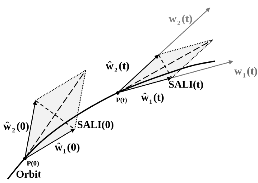
Figure 1: Schematic representation of the evolution of two deviation vectors and of the corresponding SALI for a chaotic orbit. Two initially distinct unit deviation vectors $\hat{\vec{w}}_{1}(0)$, $\hat{\vec{w}}_{2}(0)$ from point $P(0)$ of a chaotic orbit become $\vec{w}_{1}(t)$, $\vec{w}_{2}(t)$ after some time $t>0$ when the orbit reaches point $P(t)$, with $\hat{\vec{w}}_{1}(t)$, $\hat{\vec{w}}_{2}(t)$ being the unit vectors along these directions. The length of the shortest diagonals of the grey-shaded parallelograms defined by $\hat{\vec{w}}_{1}(0)$, $\hat{\vec{w}}_{2}(0)$ and $\hat{\vec{w}}_{1}(t)$, $\hat{\vec{w}}_{2}(t)$ are the values of the SALI$(0)$ and the SALI$(t)$ respectively

In the particular case shown in Fig. 1 the two unit vectors tend to align by becoming equal. This means that $\|\hat{\vec{w}}_{1}(t)-\hat{\vec{w}}_{2}(t)\|\rightarrow 0$ and $\|\hat{\vec{w}}_{1}(t)+\hat{\vec{w}}_{2}(t)\|\rightarrow 2$. Of course the dynamics could have led the vectors to become opposite. In that case we get $\|\hat{\vec{w}}_{1}(t)-\hat{\vec{w}}_{2}(t)\|\rightarrow 2$ and $\|\hat{\vec{w}}_{1}(t)+\hat{\vec{w}}_{2}(t)\|\rightarrow 0$. Since we are not interested in the particular orientation of the deviation vectors, i.e. whether they become equal or opposite to each other, when we check their possible alignment, a rather natural choice is to define the minimum of norms $\|\hat{\vec{w}}_{1}(t)+\hat{\vec{w}}_{2}(t)\|$, $\|\hat{\vec{w}}_{1}(t)-\hat{\vec{w}}_{2}(t)\|$ as an indicator of the vectors’ alignment. This is the reason of the appellation, as well as of the definition of the SALI in S_01 as

$$\mbox{SALI}(t)=\min\left\{\|\hat{\vec{w}}_{1}(t)+\hat{\vec{w}}_{2}(t)\|,\|\hat{\vec{w}}_{1}(t)-\hat{\vec{w}}_{2}(t)\|\right\},$$ (8)

with $\hat{\vec{w}}_{i}(t)=\frac{\vec{w}_{i}(t)}{\|\vec{w}_{i}(t)\|}$, $i=1,2$ being unit vectors.

Naturally, in order for the SALI to be efficiently used as a chaos indicator it should exhibit distinct behaviors for chaotic and regular orbits. As explained before the SALI becomes zero for chaotic orbits. On the other hand, in the case of regular orbits deviation vectors fall on the tangent space of the torus on which motion occurs, having in general different directions as there is no reason for them to be aligned VCE_98 ; SABV_03 . This behavior is shown schematically in Fig. 2. Thus, in this case the index should be always different from zero. In practice, the values of the SALI exhibit bounded fluctuations around some constant, positive number.

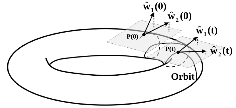
Figure 2: Schematic representation of the evolution of two deviation vectors for a regular orbit. The motion takes place on a torus. We consider two initially distinct unit deviation vectors $\hat{\vec{w}}_{1}(0)$, $\hat{\vec{w}}_{2}(0)$ from point $P(0)$, which are not necessarily on the tangent space of the torus (this space is depicted as a shaded parallelogram passing through $P(0)$). As time evolves the deviation vectors tend to fall on the torus’ tangent space and the corresponding unit vectors $\hat{\vec{w}}_{1}(t)$, $\hat{\vec{w}}_{2}(t)$ at time $t>0$ are ‘closer’ to the current tangent space (i.e. the grey-shaded parallelogram passing through $P(t)$), as the shortening of the perpendicular to the tangent spaces dotted lines from the edges of the deviation vectors indicate. Since there is no reason for the alignment of the two deviation vectors, the SALI will not become zero

Thus, in order to compute the SALI we follow the evolution of two initially distinct, random, unit deviation vectors $\hat{\vec{w}}_{1}(0)$, $\hat{\vec{w}}_{2}(0)$. Choosing these vectors to be also orthogonal sets the initial SALI to its highest possible value (SALI$(0)=\sqrt{2}$) and ensures that they are considerably different from each other, which has proved to be a very good computational practice. Then, every $t=\tau$ time units we normalize the evolved vectors $\vec{w}_{1}(i\tau)$, $\vec{w}_{2}(i\tau)$, $i=1,2,\ldots$, to $\hat{\vec{w}}_{1}(i\tau)$, $\hat{\vec{w}}_{2}(i\tau)$ and evaluate the SALI$(i\tau)$ from (8). This algorithm is described in pseudo-code in Table 1 of the Appendix. A MAPLE code for this algorithm, developed specifically for the Hénon-Heiles system (4) can be found in Chap. 5 of BS_12 .

The completely different behaviors of the SALI for regular and chaotic orbits are clearly seen in Fig. 3, where some representative results are shown for the 2D Hamiltonian system (4) and the 6d symplectic map

$$\begin{array}[]{ccl}\displaystyle x^{\prime}_{1}&\displaystyle=&\displaystyle x_{1}+y^{\prime}_{1}\\ \displaystyle y^{\prime}_{1}&\displaystyle=&\displaystyle y_{1}+\frac{K}{2\pi}\sin\left(2\pi x_{1}\right)-\frac{\gamma}{2\pi}\left\{\sin\left[2\pi\left(x_{2}-x_{1}\right)\right]+\sin\left[2\pi\left(x_{3}-x_{1}\right)\right]\right\}\\ \displaystyle x^{\prime}_{2}&\displaystyle=&\displaystyle x_{2}+y^{\prime}_{2}\\ \displaystyle y^{\prime}_{2}&\displaystyle=&\displaystyle y_{2}+\frac{K}{2\pi}\sin\left(2\pi x_{2}\right)-\frac{\gamma}{2\pi}\left\{\sin\left[2\pi\left(x_{3}-x_{2}\right)\right]+\sin\left[2\pi\left(x_{1}-x_{2}\right)\right]\right\}\\ \displaystyle x^{\prime}_{3}&\displaystyle=&\displaystyle x_{3}+y^{\prime}_{3}\\ \displaystyle y^{\prime}_{3}&\displaystyle=&\displaystyle y_{3}+\frac{K}{2\pi}\sin\left(2\pi x_{3}\right)-\frac{\gamma}{2\pi}\left\{\sin\left[2\pi\left(x_{1}-x_{3}\right)\right]+\sin\left[2\pi\left(x_{2}-x_{3}\right)\right]\right\},\end{array}$$ (9)

obtained by considering $M=3$ coupled standard maps with $K_{1}=K_{2}=K_{3}=K$ in (7). From the results of Fig. 3 we see that for both systems the SALI of regular orbits (black, solid curves) remains practically constant and positive, i.e.

$$\mbox{SALI}\propto\mbox{constant}.$$ (10)

On the other hand, the SALI of chaotic orbits (black, dashed curve in Fig. 3(a) and grey, solid curve in Fig. 3(b)) exhibits a fast decrease to zero after an initial transient time interval, reaching very small values around the computer’s accuracy ($10^{-16}$). Actually, it was shown in SABV_04 that the SALI tends to zero exponentially fast in such cases, following the law

$$\mbox{SALI}(t)\propto\exp{\left[-(\lambda_{1}-\lambda_{2})t\right]},$$ (11)

where $\lambda_{1}$, $\lambda_{2}$ ($\lambda_{1}\geq\lambda_{2}$) are the first (i.e. the mLE) and the second largest LEs respectively. As an example demonstrating the validity of this exponential-decay law we plot in Fig. 4 the evolution of the SALI (solid curve) of the chaotic orbit of Fig. 3(a) using a linear horizontal axis for time $t$. Since for 2D Hamiltonian systems $\lambda_{2}=0$, (11) becomes

$$\mbox{SALI}(t)\propto\exp{\left(-\lambda_{1}t\right)},$$ (12)

For this particular orbit the mLE was found to be $\lambda_{1}\approx 0.047$ in SABV_04 . From Fig. 4 we see that (12) with $\lambda_{1}=0.047$ (dashed line) reproduces correctly the evolution of the ALI.

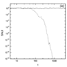
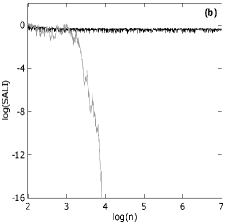
Figure 3: The time evolution of the SALI for a regular and a chaotic orbit of (a) the 2D Hamiltonian system (4) for $H_{2}=0.125$ (after SABV_04 ) and (b) the 6d map (9) for $K=3$ and $\gamma=0.1$ (after S_01 ). In (a) the time $t$ is continuous, while in (b) it is discrete and counts the map’s iterations $n$. The initial conditions of the orbits are: (a) $q_{1}=0$, $q_{2}=0.1$, $p_{1}=0.49058$, $p_{2}=0$ (regular orbit; solid curve) and $q_{1}=0$, $q_{2}=-0.25$, $p_{1}=0.42081$, $p_{2}=0$ (chaotic orbit; dashed curve), and (b) $x_{1}=0.55$, $y_{1}=0.05$, $x_{2}=0.55$, $y_{2}=0.01$, $x_{3}=0.55$, $y_{3}=0$ (regular orbit; black curve) and $x_{1}=0.55$, $y_{1}=0.05$, $x_{2}=0.55$, $y_{2}=0.21$, $x_{3}=0.55$, $y_{3}=0$ (chaotic orbit; grey curve)

t]

Figure 4: The evolution of the SALI (solid curve) for the chaotic orbit of Fig. 3(a) as a function of time $t$. The dashed line corresponds to a function proportional to $\exp{\left(-\lambda_{1}t\right)}$ for $\lambda_{1}=0.047$. Note that the $t$-axis is linear (after SABV_04 )

Thus, the completely different behavior of the SALI for regular (10) and chaotic (11) orbits permits the clear and efficient distinction between the two cases. In S_01 ; SABV_04 a comparison of the SALI’s performance with respect to other chaos detection techniques was presented and the efficiency of the index was discussed. A main advantage of the SALI method is its ability to detect chaotic motion faster than other techniques which depend on the whole time evolution of deviation vectors, like the mLE and the spectral distance, because the SALI is determined by the current state of these vectors and is not influenced by their evolution history. Hence, the moment the two vectors are close enough to each other the SALI becomes practically zero and guarantees the chaotic nature of the orbit beyond any doubt. In addition, the evaluation of the SALI is simpler and more straightforward with respect to other methods that require more complicated computations. Such aspects were discussed in SABV_04 where a comparison of the index with the Relative Lyapunov Indicator (RLI) SESF_04 and the so-called ‘0–1’ test GM_04 was presented. Another crucial characteristic of the SALI is that it attains values in a given interval, namely SALI$(t)\in[0,\sqrt{2}]$, which does not change in time as is for example the case for the Fast Lyapunov Indicator (FLI) FGL_97 . Thus, setting a realistic threshold value below which the SALI is considered to be practically zero (and the corresponding orbit is characterized as chaotic), allows the fast and accurate discrimination between regular and chaotic motion. Due to all these features the SALI became a reliable and widely used chaos indicator as its numerous applications to a variety of dynamical systems over the years prove. Some of these applications are discussed in Sect. 4.

3 The Generalized Alignment Index (GALI)

A fundamental difference between the SALI and other, commonly applied chaos indicators, is that it uses information from the evolution of two deviation vectors instead of just one. A consequence of this feature is the appearance of the two largest LEs in (11). After performing this first leap from using only one deviation vector, the question of going even further arises naturally. To formulate this in other words: why should we stop in using only two deviation vectors? Can we extend the definition of the SALI to include more deviation vectors? Assuming that this extension is possible, what will we gain from it? Will the use of more than two deviation vectors lead to the introduction of a new chaoticity index which will permit the acquisition of a deeper understanding of the system’s dynamics, exhibiting at the same time a better numerical performance than the SALI? For instance, from (11) we realize that in the case of a chaotic orbit with $\lambda_{1}\approx\lambda_{2}$ the convergence of the SALI to zero will be extremely slow. As a result long integrations would be required in order for the index to distinguish this orbit from a regular one for which the SALI remains practically constant. Although the existence of such chaotic orbits is not very probable the drawback of the SALI remains. An alternative way to state this problem is the following: can we construct a new index whose behavior in the case of chaotic orbits will depend on more LEs than the two largest ones so that it can overcome the discrimination problem for $\lambda_{1}\approx\lambda_{2}$?

Indeed, such an index can be constructed. The key point to its development is the observation that the SALI is closely related to the area of the parallelogram defined by the two deviation vectors. From the schematic representation of the deviation vectors’ evolution in Fig. 1 we see that when the SALI vanishes one of the diagonals of the parallelogram also vanishes, and consequently its area becomes zero. The area $A_{2}$ of a usual 2d parallelogram is equal to the norm of the exterior product of its two sides $\vec{v}_{1}$, $\vec{v}_{2}$, and also equal to the half of the product of its diagonals’ lengths

$$A_{2}=\|\vec{v}_{1}\times\vec{v}_{2}\|=\frac{\|\vec{v}_{1}+\vec{v}_{2}\|\cdot\|\vec{v}_{1}-\vec{v}_{2}\|}{2}.$$ (13)

In a similar way, the area $A$ of the parallelogram of Fig. 1 is given by the generalization of the exterior product of vectors to higher dimensions, i.e. the so-called wedge product denoted by $(\wedge)$, so that

$$A=\|\hat{\vec{w}}_{1}\wedge\hat{\vec{w}}_{2}\|=\frac{\|\hat{\vec{w}}_{1}+\hat{\vec{w}}_{2}\|\cdot\|\hat{\vec{w}}_{1}-\hat{\vec{w}}_{2}\|}{2}.$$ (14)

Note the analogy of this equation to (13).

Based on the fact that the SALI is related to the area of the parallelogram defined by two unit deviation vectors, the extension of the index to include more vectors is straightforward: the new quantity is defined as the volume of the parallelepiped formed by more than two deviation vectors. This volume is computed as the norm of the wedge product of these vectors. These arguments led to the introduction in SBA_07 of the Generalized Alignment Index of order $k$ (GALI_k) as

$$\mbox{GALI}_{k}(t)=\|\hat{\vec{w}}_{1}(t)\wedge\hat{\vec{w}}_{2}(t)\wedge\ldots\wedge\hat{\vec{w}}_{k}(t)\|,$$ (15)

where $\hat{\vec{w}}_{i}$ are unit vectors as in (8). In this definition the number of used deviation vectors should not exceed the dimension of the system’s phase space, because in this case the $k$ vectors will become linearly dependent and the corresponding volume will be by definition zero, as is for example the area defined by two vectors having the same direction. Thus, for an $N$D Hamiltonian system with $N\geq 2$ or a $2N$d symplectic map with $N\geq 1$, we consider only GALIs with $2\leq k\leq 2N$.

By its definition the GALI_k is a quantity clearly indicating the linear dependence (GALI${}_{k}=0$) or independence (GALI${}_{k}>0$) of $k$ deviation vectors. The SALI has the same discriminating ability as SALI$=0$ indicates that the two vectors are aligned, i.e. they are linearly dependent, while $\mbox{SALI}>0$ implies that the vectors are not aligned, which means that they are linearly independent. Actually, the connection between the two indices can be quantified explicitly. Indeed, it was proved in the Appendix B of SBA_07 that

$$\mbox{GALI}_{2}=\mbox{SALI}\cdot\frac{\max\left\{\|\hat{\vec{w}}_{1}(t)+\hat{\vec{w}}_{2}(t)\|,\|\hat{\vec{w}}_{1}(t)-\hat{\vec{w}}_{2}(t)\|\right\}}{2}.$$ (16)

Since the $\max\left\{\|\hat{\vec{w}}_{1}(t)+\hat{\vec{w}}_{2}(t)\|,\|\hat{\vec{w}}_{1}(t)-\hat{\vec{w}}_{2}(t)\|\right\}$ is a number in the interval $[\sqrt{2},2]$ we conclude that

$$\mbox{GALI}_{2}\propto\mbox{SALI},$$ (17)

which means that the GALI₂ is practically equivalent to the SALI. This is another evidence that the GALI definition (15) is a natural extension of the SALI for more than two deviation vectors.

3.1 Computation of the GALI

Let us discuss now how one can actually calculate the value of the GALI_k for an $N$D Hamiltonian system ($N\geq 2$) or a $2N$d symplectic map ($N\geq 1$). For this purpose we consider the $k\times 2N$ matrix

$$\textbf{A}(t)=\left[\begin{array}[]{cccc}w_{11}(t)&w_{12}(t)&\cdots&w_{1\,2N}(t)\\ w_{21}(t)&w_{22}(t)&\cdots&w_{2\,2N}(t)\\ \vdots&\vdots&&\vdots\\ w_{k1}(t)&w_{k2}(t)&\cdots&w_{k\,2N}(t)\end{array}\right]$$ (18)

having as rows the $2N$ coordinates of the $k$ unit deviation vectors $\hat{\vec{w}}_{i}(t)$ with respect to the usual orthonormal basis $\hat{\vec{e}}_{1}=(1,0,0,\ldots,0)$, $\hat{\vec{e}}_{2}=(0,1,0,\ldots,0)$, …, $\hat{\vec{e}}_{2N}=(0,0,0,\ldots,1)$. We note that the elements of $\textbf{A}(t)$ satisfy the condition $\sum_{j=1}^{2N}w_{ij}^{2}(t)=1$ for $i=1,2,\ldots,k$ as each deviation vector has unit norm.

We can now follow two routes for evaluating the GALI${}_{k}(t)$. According to the first one we compute the GALI_k by evaluating the norm of the wedge product of $k$ vectors as

$$\mbox{GALI}_{k}(t)=\left\{\sum_{1\leq i_{1}<i_{2}<\cdots<i_{k}\leq 2N}\left(\det\left[\begin{array}[]{cccc}w_{1i_{1}}(t)&w_{1i_{2}}(t)&\cdots&w_{1i_{k}}(t)\\ w_{2i_{1}}(t)&w_{2i_{2}}(t)&\cdots&w_{2i_{k}}(t)\\ \vdots&\vdots&&\vdots\\ w_{ki_{1}}(t)&w_{ki_{2}}(t)&\cdots&w_{ki_{k}}(t)\end{array}\right]\right)^{2}\right\}^{1/2},$$ (19)

where the sum is performed over all the possible combinations of $k$ indices out of $2N$ (a proof of this equation can be found in SBA_07 ). In practice this means that in our calculation we consider all the $k\times k$ determinants of $\textbf{A}(t)$. Equation (19) is particularly useful for the theoretical description of the GALI’s behavior (actually expressions (22) and (23) below were obtained by using this equation), but not very efficient from a practical point of view. The reason is that the number of determinants appearing in (19) can increase enormously when $N$ grows, leading to unfeasible numerical computations.

A simpler, straightforward and computationally more efficient approach to evaluate the GALI_k was developed in SBA_08 , where it was proved that the index is equal to the product of the singular values $z_{i}$, $i=1,2,\ldots,k$ of $\textbf{A}^{T}(t)$ (the transpose of matrix $\textbf{A}(t)$), i.e.

$$\mbox{GALI}_{k}(t)=\prod_{i=1}^{k}z_{i}(t).$$ (20)

We note that the singular values of $\textbf{A}^{T}(t)$ are obtained by performing the Singular Value Decomposition (SVD) procedure to $\textbf{A}^{T}(t)$. According to the SVD method (see for instance Sect. 2.6 of NumRec ) the $2N\times k$ matrix $\textbf{A}^{T}$ is written as the product of a $2N\times k$ column-orthogonal matrix U ($\textbf{U}^{T}\cdot\textbf{U}=\textbf{I}_{k}$, with $\textbf{I}_{k}$ being the $k\times k$ unit matrix), a $k\times k$ diagonal matrix Z having as elements the positive or zero singular values $z_{i}$, $i=1,\ldots,k$, and the transpose of a $k\times k$ orthogonal matrix V ($\textbf{V}^{T}\cdot\textbf{V}=\textbf{I}_{k}$), i.e.

$$\textbf{A}^{\mathrm{T}}=\textbf{U}\cdot\textbf{Z}\cdot\textbf{V}^{\mathrm{T}}.$$ (21)

In practice, in order to compute the GALI of order $k$ we follow the evolution of $k$ initially distinct, random, orthonormal deviation vectors $\hat{\vec{w}}_{1}(0)$, $\hat{\vec{w}}_{2}(0)$, $\ldots$, $\hat{\vec{w}}_{k}(0)$. Similarly to the computation of the SALI, choosing orthonormal vectors ensures that all of them are sufficiently far from linear dependence and gives to the GALI_k its largest possible initial value GALI${}_{k}=1$. Afterwards, every $t=\tau$ time units we normalize the evolved vectors $\vec{w}_{1}(i\tau)$, $\vec{w}_{2}(i\tau)$, $\ldots$, $\vec{w}_{k}(i\tau)$, $i=1,2,\ldots$, to $\hat{\vec{w}}_{1}(i\tau)$, $\hat{\vec{w}}_{2}(i\tau)$, $\ldots$, $\hat{\vec{w}}_{k}(i\tau)$ and set them as rows of a matrix $\textbf{A}(i\tau)$ (18). Then, according to (20) the GALI${}_{k}(i\tau)$ is computed as the product of the singular values of matrix $\textbf{A}^{T}(i\tau)$. This algorithm is described in pseudo-code in Table 2 of the Appendix. A MAPLE code computing all the possible GALIs (i.e. GALI₂, GALI₃ and GALI₄) for the 2D Hamiltonian (4) can be found in Chap. 5 of BS_12 .

3.2 Behavior of the GALI for Chaotic and Regular Orbits

After defining the new index and explaining a practical way to evaluate it, let us discuss its ability to discriminate between chaotic and regular motion. As we have already mentioned, in the case of a chaotic orbit all deviation vectors eventually become aligned to the direction defined by the largest LE. Thus, they become linearly dependent and consequently the volume they define vanishes, meaning that the GALI_k, $2\leq k\leq 2N$, will become zero. Actually, in SBA_07 it was shown analytically that in this case the the GALI${}_{k}(t)$ decreases to zero exponentially fast with an exponent which depends on the $k$ largest LEs as

$$\mbox{GALI}_{k}(t)\propto\exp\left\{-\left[(\lambda_{1}-\lambda_{2})+(\lambda_{1}-\lambda_{3})+\cdots+(\lambda_{1}-\lambda_{k})\right]t\right\}.$$ (22)

Note that for $k=2$ we get the exponential law (11) in agreement with the equivalence between the GALI₂ and the SALI (17).

Let us now consider the case of regular motion in a $N$D Hamiltonian system or a 2$N$d symplectic map with $N\geq 2$. In general, this motion occurs on an $N$d torus in the system’s 2$N$d phase space. As we discussed in Sect. 2, in this case any deviation vector eventually falls on the $N$d tangent space of the torus (Fig. 2). Consequently, the $k$ initially distinct, linearly independent deviation vectors we follow in order to compute the evolution of the GALI_k eventually falls on the $N$d tangent space of the torus, without necessarily having the same directions. Thus, if we do not consider more deviation vectors than the dimension of the tangent space ($k\leq N$) we end up with $k$ linearly independent vectors on the torus’ tangent space and consequently the volume of the parallelepiped they define (i.e. the GALI_k) will be different from zero. As we see later on, numerical simulations show that the GALI_k exhibits small fluctuations around some positive value. If, on the other hand, we consider more deviation vectors than the dimension of the tangent space ($N<k\leq 2N$) the deviation vectors eventually become linearly dependent, as we end up with more vectors in the torus’ tangent space than the space’s dimension. Thus, the volume that these vectors define will vanish and the GALI_k will become zero. Specifically, in SBA_07 it was shown analytically that in this case the GALI_k tends to zero following a power law whose exponent depends on the torus dimension and on the number $k$ of deviation vectors considered, i.e. GALI${}_{k}\propto t^{-2(k-N)}$. In summary the behavior of the GALI_k for regular orbits is

$$\mbox{GALI}_{k}(t)\propto\left\{\begin{array}[]{ll}\mbox{constant}&\mbox{if $2\leq k\leq N$ }\\ \frac{1}{t^{2(k-N)}}&\mbox{if $N<k\leq 2N.$}\\ \end{array}\right.$$ (23)

From this equation we see that $\mbox{SALI}\propto\mbox{GALI}_{2}\propto\mbox{constant}$, in accordance to (10).

Some Illustrative Paradigms

In what follows we illustrate the different behaviors of the GALI_k by computing its evolution for some representative chaotic and regular orbits of various $N$D autonomous Hamiltonians and 2$N$d symplectic maps. Before doing so let us note that for these systems the LEs comes in pairs of values having opposite signs

$$\lambda_{i}=-\lambda_{2N-i+1},\,\,\,\,i=1,2,\ldots,N,$$ (24)

while, moreover

$$\lambda_{N}=\lambda_{N+1}=0$$ (25)

for Hamiltonian systems BGGS_80a ; H_83 ; S_10 .

Hamiltonian systems

Initially, we consider the 2D Hamiltonian (4) which has a 4d phase space. For this system we can define the GALI_k for $k=2$, 3 and 4. Then, according to (24) and (25), the LEs satisfy the conditions $\lambda_{1}=-\lambda_{4}$, $\lambda_{2}=\lambda_{3}=0$. Thus, according to (22) the evolution of the GALIs for a chaotic orbit is given by

$$\mbox{GALI}_{2}(t)\propto e^{-\lambda_{1}t},\,\,\,\mbox{GALI}_{3}(t)\propto e^{-2\lambda_{1}t},\,\,\,\mbox{GALI}_{4}(t)\propto e^{-4\lambda_{1}t}.$$ (26)

On the other hand, for a regular orbit (23) indicates that

$$\mbox{GALI}_{2}(t)\propto\mbox{constant},\,\,\,\mbox{GALI}_{3}(t)\propto\frac{1}{t^{2}},\,\,\,\mbox{GALI}_{4}(t)\propto\frac{1}{t^{4}}.$$ (27)

From the results of Fig. 5, where the time evolution of the GALI₂, the GALI₃ and the GALI₄ for a chaotic orbit (actually the one considered in Figs. 3(a) and 4) and a regular orbit are plotted, we see that the laws (26) and (27) describe quite accurately the obtained numerical data.

     

Figure 5: The time evolution of the GALI₂, the GALI₃ and the GALI₄ for (a) a chaotic and (b) a regular orbit of the 2D Hamiltonian (4) for $H_{2}=0.125$. The chaotic orbit is the one considered in Fig. 3a, while the initial conditions of the regular orbit are $q_{1}=0$, $q_{2}=0$, $p_{1}=0.5$, $p_{2}=0$. The straight lines correspond in (a) to functions proportional to $\exp(-\lambda_{1}t)$, $\exp(-2\lambda_{1}t)$ and $\exp(-4\lambda_{1}t)$, for $\lambda_{1}=0.047$ and in (b) to functions proportional to $t^{-2}$ and $t^{-4}$. The slope of each line is mentioned in the legend. Note that the horizontal, time axis in (a) is linear, while in (b) is logarithmic (after SBA_07 )

For a 3D Hamiltonian like (5) the theoretical prediction (22) gives

$$\begin{array}[]{c}\mbox{GALI}_{2}(t)\propto e^{-(\lambda_{1}-\lambda_{2})t},\,\,\,\mbox{GALI}_{3}(t)\propto e^{-(2\lambda_{1}-\lambda_{2})t},\,\,\,\mbox{GALI}_{4}(t)\propto e^{-(3\lambda_{1}-\lambda_{2})t},\vspace{0.2cm}\\ \mbox{GALI}_{5}(t)\propto e^{-4\lambda_{1}t},\,\,\,\mbox{GALI}_{6}(t)\propto e^{-6\lambda_{1}t},\end{array}$$ (28)

for a chaotic orbit, because, according to (24) and (25), $\lambda_{1}=-\lambda_{6}$, $\lambda_{2}=-\lambda_{5}$ and $\lambda_{3}=\lambda_{4}=0$. On the other hand, a regular orbit lies on a 3d torus and according to (23) the GALIs should behave as

$$\begin{array}[]{c}\displaystyle\mbox{GALI}_{2}(t)\propto\mbox{constant},\,\,\,\mbox{GALI}_{3}(t)\propto\mbox{constant},\,\,\,\mbox{GALI}_{4}(t)\propto\frac{1}{t^{2}},\\ \displaystyle\mbox{GALI}_{5}(t)\propto\frac{1}{t^{4}},\,\,\,\mbox{GALI}_{6}(t)\propto\frac{1}{t^{6}}.\end{array}$$ (29)

In Fig. 6 we plot the time evolution of the various GALIs for a chaotic (Fig. 6(a)) and a regular (Fig. 6(b)) orbit of the 3D Hamiltonian (5). From the plotted results we see that the behaviors of the GALIs are very well approximated by (28) and (29). We note here that the constant values that the GALI₂ and the GALI₃ eventually attain in Fig. 6(b) are not the same. Actually, the limiting value of GALI₃ is smaller than the one of GALI₂.

     

Figure 6: The time evolution of the GALI_k, $k=2,3,\ldots,6$ for (a) a chaotic and (b) a regular orbit of the 3D Hamiltonian (5) with $H_{3}=0.09$, $\omega_{1}=1$, $\omega_{2}=\sqrt{2}$ and $\omega_{3}=\sqrt{3}$. The initial conditions of the orbits are: (a) $q_{1}=0$, $q_{2}=0$, $q_{3}=0$, $E_{1}=0.03$, $E_{2}=0.03$, $E_{3}=0.03$, and (b) $q_{1}=0$, $q_{2}=0$, $q_{3}=0$, $E_{1}=0.005$, $E_{2}=0.085$, $E_{3}=0$, where the quantities $E_{1}$, $E_{2}$, $E_{3}$ (usually referred as the ‘harmonic energies’) are related to the momenta $p_{1}$, $p_{2}$, $p_{3}$ through $p_{i}=\sqrt{2E_{i}/\omega_{i}}$, $i=1,2,3$. The straight lines in (a) correspond to functions proportional to $\exp[-(\lambda_{1}-\lambda_{2})t]$, $\exp[-(2\lambda_{1}-\lambda_{2})t]$, $\exp[-(3\lambda_{1}-\lambda_{2})t]$, $\exp(-4\lambda_{1}t)$ and $\exp(-6\lambda_{1}t)$ for $\lambda_{1}=0.03$, $\lambda_{2}=0.008$, which are accurate numerical estimations of the orbit’s two largest LEs (see SBA_07 for more details). The straight lines in (b) correspond to functions proportional to $t^{-2}$, $t^{-4}$ and $t^{-6}$. The slope of each line is mentioned in the legend. The horizontal, time axis is linear in (a) and logarithmic in (b) (after SBA_07 )

As an example of evaluating the GALIs for multidimensional Hamiltonians we consider model (6) for $N=8$ particles. This corresponds to an 8D Hamiltonian system $H_{8}$, having a 16d phase space, which allows the definition of several GALIs: starting from GALI₂ up to GALI₁₆. In Fig. 7 the time evolution of several of these indices are shown for a chaotic (Figs. 7(a) and (b)) and a regular (Figs. 7(c) and (d)) orbit. From these results we again conclude that the laws (22) and (23) are quite accurate in describing the time evolution of the GALIs.

     

Figure 7: The time evolution of the GALI_k, $k=2,\ldots,8,10,12,14,16$ for a chaotic (panels (a) and (b)) and a regular orbit (panels (c) and (d)) of the $N$D Hamiltonian (6) with $N=8$ and $\beta=1.5$. The initial conditions of the chaotic orbit are $Q_{1}=Q_{4}=2$, $Q_{2}=Q_{5}=1$, $Q_{3}=Q_{6}=0.5$, $Q_{7}=Q_{8}=0.1$, $P_{i}=0$ where $\displaystyle Q_{i}=\frac{2}{3}\sum_{j=1}^{8}q_{j}\sin\left(\frac{ij\pi}{9}\right)$, $\displaystyle P_{i}=\frac{2}{3}\sum_{j=1}^{8}p_{j}\sin\left(\frac{ij\pi}{9}\right)$, $i=1,\ldots,8$ (see SBA_08 for more details). The initial conditions of the regular orbit are $q_{1}=q_{2}=q_{3}=q_{8}=0.05$, $q_{4}=q_{5}=q_{6}=q_{7}=0.1$, $p_{i}=0$, $i=1,\ldots,8$. The straight lines in (a) and (b) correspond to exponential functions of the form (22) for $\lambda_{1}=0.170$, $\lambda_{2}=0.141$, $\lambda_{3}=0.114$, $\lambda_{4}=0.089$, $\lambda_{5}=0.064$, $\lambda_{6}=0.042$, $\lambda_{7}=0.020$ , which are estimations (obtained in SBA_08 ) of the orbit’s seven largest LEs. The straight lines in (d) correspond to functions proportional to $t^{-4}$, $t^{-8}$, $t^{-12}$ and $t^{-16}$. The slope of each line is mentioned in the legend. Note the huge range differences in the horizontal, time axes between panels (a) and (b), where the axes are linear, and panels (c) and (d) where the axes are logarithmic (after SBA_08 )

The first seven indices, GALI₂ up to GALI₈, exhibit completely different behaviors for chaotic and regular motion: they tend exponentially fast to zero for a chaotic orbit (Figs. 7(a) and (b)), while they attain constant, positive values for a regular one (Fig. 7(c)). This characteristic makes them ideal numerical tools for discriminating between the two cases, as we see in Sect. 4.1 where some specific numerical examples are discussed in detail.

Although the constancy of the GALI_k, $k=1,\ldots,8$ for regular orbits is predicted from (23), nothing is yet said about the actual values of these constants. It is evident from Fig. 7(c) that these values decrease as the order $k$ of the GALI_k increases, something which was also observed in Fig. 6(b) for the 3D Hamiltonian (5). For the regular orbit of Fig. 7(c) we see that GALI${}_{8}\approx 10^{-7}$. One might argue that this very small value could be considered to be practically zero and that the orbit might be (wrongly) classified as chaotic. The flaw in this argumentation is that the possible smallness of GALI${}_{8}\approx 10^{-7}$ is of relative nature as this value should be compared with the values that the index reaches for actual chaotic orbits. For instance, the chaotic orbit of Fig. 7(b) has GALI${}_{8}\approx 10^{-40}$, after only $t\approx 160$ time units! At the same time we get GALI${}_{8}\approx 10^{-1}$ for the regular orbit (Fig. 7(c)). In addition, extrapolating the results of GALI₈ for the chaotic orbit in Fig. 7(b) to e.g. $t\approx 10^{5}$ we would obtain values extremely smaller than the value GALI${}_{8}\approx 10^{-7}$ archived for the regular orbit in Fig. 7(c).

The necessity to determine an appropriate threshold value for the GALI_k, $2\leq k\leq N$, below which orbits will be securely classified as chaotic, becomes evident from the above analysis. Since a theoretical, or even an empirical (numerical) relation between the order $k$ of the GALI_k and the constant value it reaches for regular orbits is still lacking, one efficient way to determine this threshold value is by computing the GALI_k for some representative chaotic and regular orbits of each studied system. Then, a safe policy is to define this threshold to be a few orders of magnitude smaller than the minimum value obtained by the GALI_k for the tested regular orbits. For example, based on the results of Fig. 6 for the 3D Hamiltonian (5) this threshold value for the GALI₃ could be set to be $\leq 10^{-8}$, while for the system of Fig. 7 a reliable threshold value for the GALI₈ could be $\leq 10^{-16}$.

The results of Fig. 7 verify the predictions of (22) and (23) that the GALIs of order $8<k\leq 16$ tend to zero both for chaotic and regular orbits. Nevertheless, the completely different way they do so, i.e. they decay exponentially fast for chaotic orbits, while they follow a power law decay for regular ones, allows us again to develop a well-tailored strategy to discriminate between the two cases. The different decay laws result in enormous differences in the time the indices need to reach any predefined low value. Thus, the measurement of this time can be used to characterize the nature of the orbits, as we see in Sect. 4.1. For example, for the chaotic orbit of Fig. 7(b) GALI${}_{16}\approx 10^{-30}$ after about $t\approx 25$ time units, while it reaches the same small value after about $t\approx 10^{5}$ time units for the regular orbit of Fig. 7(d); a time interval which is larger by a factor $\approx 4,000$ with respect to the chaotic orbit!

Symplectic Maps

Although up to now our discussion concerned the implementation of the GALIs to Hamiltonian systems, the indices follow laws (22) and (23) also for symplectic maps (with the obvious substitution of the continuous time $t$ by a discrete one which counts the map’s iterations $n$) as the representative results of Figs. 8 and 9 clearly verify. In particular, in Fig. 8 we see the behavior of the GALIs for a chaotic (Fig. 8(a)) and a regular (Fig. 8(b)) orbit of the 4d map

$$\begin{array}[]{ccl}\displaystyle x^{\prime}_{1}&\displaystyle=&\displaystyle x_{1}+y^{\prime}_{1}\\ \displaystyle y^{\prime}_{1}&\displaystyle=&\displaystyle y_{1}+\frac{K}{2\pi}\sin\left(2\pi x_{1}\right)-\frac{\gamma}{2\pi}\sin\left[2\pi\left(x_{2}-x_{1}\right)\right]\\ \displaystyle x^{\prime}_{2}&\displaystyle=&\displaystyle x_{2}+y^{\prime}_{2}\\ \displaystyle y^{\prime}_{2}&\displaystyle=&\displaystyle y_{2}+\frac{K}{2\pi}\sin\left(2\pi x_{2}\right)-\frac{\gamma}{2\pi}\sin\left[2\pi\left(x_{1}-x_{2}\right)\right],\end{array}$$ (30)

obtained from (7) for $M=2$ and $K_{1}=K_{2}=K$, while in Fig. 9 a chaotic (Fig. 9(a)) and a regular (Fig. 9(b)) orbit of the 6d map (9) are considered.

     

Figure 8: The evolution of the GALI₂, the GALI₃ and the GALI₄ with respect to the number of iterations $n$ for (a) a chaotic and (b) a regular orbit of the 4d map (30) with $K=0.5$ and $\gamma=0.05$. The initial conditions of the orbits are: (a) $x_{1}=0.55$, $y_{1}=0.1$, $x_{2}=0.005$, $y_{2}=0.01$, and (b) $x_{1}=0.55$, $y_{1}=0.1$, $x_{2}=0.54$, $y_{2}=0.01$. The straight lines in (a) correspond to functions proportional to $\exp[-(\lambda_{1}-\lambda_{2})n]$, $\exp(-2\lambda_{1}n)$ and $\exp(-4\lambda_{1}n)$ for $\lambda_{1}=0.07$, $\lambda_{2}=0.008$, which are the orbit’s LEs obtained in MSB_09 . The straight lines in (b) represent functions proportional to $n^{-2}$ and $n^{-4}$. The slope of each line is mentioned in the legend. Note that the horizontal axis is linear in (a) and logarithmic in (b) (after MSB_09 )

     

Figure 9: The evolution of the GALI_k, $k=2,3,\ldots,6$ with respect to the number of iterations $n$ for (a) a chaotic (after MSB_08 ) and (b) a regular orbit of the 6d map (9) with $K=3$ and $\gamma=0.1$. The initial conditions of the orbits are: (a) $x_{1}=x_{2}=x_{3}=0.8$, $y_{1}=0.05$, $y_{2}=0.21$, $y_{3}=0.01$, and (b) $x_{1}=x_{2}=x_{3}=0.55$, $y_{1}=0.05$, $y_{2}=0.21$, $y_{3}=0$. The straight lines in (a) correspond to functions proportional to $\exp[-(\lambda_{1}-\lambda_{2})n]$, $\exp[-(2\lambda_{1}-\lambda_{2}-\lambda_{3})n]$, $\exp[-(3\lambda_{1}-\lambda_{2})n]$, $\exp(-4\lambda_{1}n)$ and $\exp(-6\lambda_{1}n)$ for $\lambda_{1}=0.70$, $\lambda_{2}=0.57$, $\lambda_{3}=0.32$, which are the orbit’s LEs obtained in MSB_08 . The straight lines in (b) represent functions proportional to $n^{-2}$, $n^{-4}$ and $n^{-6}$. The slope of each line is mentioned in the legend. Note that the horizontal axis is linear in (a) and logarithmic in (b)

These results illustrate the fact that the GALI_k has the same behavior for Hamiltonian flows and symplectic maps. For instance, even by simple inspection we conclude that the GALIs behave similarly in Figs. 5 and 8, which refer to a 2D Hamiltonian and a 4d map respectively, as well as in Figs. 6 and 9, which refer to a 3D Hamiltonian and a 4d map respectively.

The Case of 2d Maps

Equations (22) and (23) describe the behavior of the GALIs for $N$D Hamiltonian systems and $2N$d symplectic maps with $N\geq 2$. What happens if $N=1$? The case of an 1D, time independent Hamiltonian is not very interesting because such systems are integrable and chaos does not appear. But, this is not the case for 2d maps, which can exhibit chaotic behavior.

In 2d maps only the GALI₂ (which, according to (17) is equivalent to the SALI) is defined. For chaotic orbits the GALI₂ decreases exponentially to zero according to (22), which becomes

$$\mbox{GALI}_{2}(n)\propto\mbox{SALI}(n)\propto\exp\left(-2\lambda_{1}n\right),$$ (31)

in this particular case, since, according to (24) $\lambda_{1}=-\lambda_{2}>0$. Note that in (31) we have substituted the continuous time $t$ of (22) by the number $n$ of map’s iterations. The agreement between the prediction (31) and actual, numerical data can be seen for example in Fig. 10(a) where the evolution of the SALI ($\propto\mbox{GALI}_{2}$) is plotted for a chaotic orbit of the 2d standard map

$$\begin{array}[]{ccl}\displaystyle x^{\prime}_{1}&\displaystyle=&\displaystyle x_{1}+y^{\prime}_{1}\\ \displaystyle y^{\prime}_{1}&\displaystyle=&\displaystyle y_{1}+\frac{K}{2\pi}\sin\left(2\pi x_{1}\right),\end{array}$$ (32)

obtained from (7) for $M=1$. Thus, we conclude that (22) is also valid for 2d maps.

                   

Figure 10: The evolution of the SALI (which in practice is the GALI₂) with respect to the number of iterations $n$ for (a) a chaotic and (b) a regular orbit of the 2d map (32) with $K=2$. The initial conditions of the orbits are: (a) $x_{1}=y_{1}=0.2$, and (b) $x_{1}=0.4$, $y_{1}=0.8$. The straight line in (a) corresponds to a function proportional to $\exp(-2\lambda_{1}n)$ for $\lambda_{1}=0.438$, which is the orbit’s mLE obtained in MSAB2008 , while the line in (b) represents a function proportional to $n^{-2}$. The slope of each line is mentioned in the legend. Note that the horizontal axis is linear in (a) and logarithmic in (b) (after MSAB2008 )

But what happens in the case of regular orbits? Is (23) still valid for $k=2$ and $N=1$? First of all let us note that for these particular values of $k$ and $N$ only the second branch of (23) is meaningful, and it provides the prediction that the GALI₂ tends to zero as $n^{-2}$. This result is interesting, as this is the first case of regular motion for which no GALI remains constant. But actually the vanishing of the GALI₂ in this case is not surprising. Regular motion in 2d maps occurs on 1d invariant curves. So, any deviation vector from a regular orbit eventually falls on the tangent space of this curve, which of course has dimension 1. Thus, the two deviation vectors needed for the computation of the GALI₂ eventually becomes collinear and consequently GALI${}_{2}\rightarrow 0$. Actually the prediction obtained by (23), that for regular orbits of 2d maps

$$\mbox{GALI}_{2}(n)\propto\mbox{SALI}(n)\propto\frac{1}{n^{2}},$$ (33)

is correct, as for example the results of Fig. 10(b) show.

In conclusion we note that the behavior of the SALI/GALI₂ for chaotic and regular orbits in 2d maps is respectively given by (31) and (33), which are obtained from (22) and (23) for $k=2$ and $N=1$. The different behaviors of the index for chaotic (exponential decay) and regular motion (power law decay) were initially observed in S_01 , although the exact functional laws (31) and (33) were derived later SABV_04 ; SBA_07 . As was pointed out even from the first paper on the SALI S_01 , these differences allow us to use the SALI/GALI₂ to distinguish between chaotic and regular motion also in 2d maps (see for instance S_01 ; MSAB2008 ).

3.3 Regular Motion on Low Dimensional Tori

An important feature of the GALIs is their ability to identify regular motion on low dimensional tori. In order to explain this capability let us assume that a regular orbit lies on an $s$d torus, $2\leq s\leq N$, in the $2N$d phase space on an $N$D Hamiltonian system or a $2N$d map with $N\geq 2$. Then, following similar arguments to the ones made in Sect. 3.2 for regular motion on an $N$d torus, we conclude that the GALI_k eventually remains constant for $2\leq k\leq s$, because in this case the $k$ deviation vectors will remain linearly independent when they eventually fall on the $s$d tangent space of the torus. On the other hand, any $s<k\leq 2N$ deviation vectors eventually become linearly dependent as there will be more vectors on the torus’ tangent space than the space’s dimension, and consequently the GALI_k will vanish. In this case, the way the GALI_k tends to zero depends not only on $k$ and $N$, as in (23), but also on the dimension $s$ of the torus. Actually, it was shown analytically in CB2006 ; SBA_08 that for regular orbits on an $s$d torus the GALI_k behaves as

$$\mbox{GALI}_{k}(t)\propto\left\{\begin{array}[]{ll}\mbox{constant}&\mbox{if $2\leq k\leq s$}\\ \frac{1}{t^{k-s}}&\mbox{if $s<k\leq 2N-s$}\\ \frac{1}{t^{2(k-N)}}&\mbox{if $2N-s<k\leq 2N.$}\\ \end{array}\right.$$ (34)

It is worth noting that for $s=N$ we retrieve (23) as the second branch of (34) becomes meaningless, while by setting $k=2$, $s=1$ and $N=1$ we get (33).

The validity of (34) is supported by the results of Fig. 11 where two representative regular orbits of the $H_{8}$ Hamiltonian, obtained by setting $N=8$ in (6), are considered (we note that Fig. 7 refers to the same model). The first orbit (Figs. 11(a) and (b)) lies on a 2d torus as the constancy of only GALI₂ indicates. The decay of the remaining GALIs is well reproduced by the power laws (34) for $N=8$ and $s=2$. The second orbit (Figs. 11(c) and (d)) lies on a 4d torus and consequently the GALI₂, the GALI₃ and the GALI₄ remain constant, while all other indices follow power law decays according to (34) for $N=8$ and $s=4$.

     

Figure 11: The time evolution of the GALI_k, $k=2,\ldots,9,11,13,14,16$ for a regular orbit lying on a 2d torus (panels (a) and (b)) and for another one lying on a 4d torus (panels (c) and (d)) of the 8D Hamiltonian $H_{8}$ considered in Fig. 7. The initial conditions of the first orbit are $Q_{1}=2$, $P_{1}=0$, $Q_{i}=P_{i}=0$, $i=2,\ldots,8$ (the definition of these variables is given in the caption of Fig. 7). The initial conditions of the second orbit are $q_{i}=0.1$, $p_{i}=0$, $i=1,\ldots,8$. The plotted straight lines correspond to the power law predictions (34) for $N=8$, $s=2$ (panels (a) and (b)) and for $N=8$, $s=4$ (panels (c) and (d)). The slope of each line is mentioned in the legend (after SBA_08 )

In Fig. 12 we see the evolution of some GALIs for regular motion on low dimensional tori of the 40d map obtained by (7) for $M=20$. The results of Fig. 12(a) denote that the orbit lies on a 3d torus in the 40d phase space of the map, while in the case of Fig. 12(b) the motion takes place on a 6d torus. The plotted straight lines help us verify that for both orbits the behaviors of the decaying GALIs are accurately reproduced by (34) for $N=20$, $s=3$ (Fig. 12(a)) and $N=20$, $s=6$ (Fig. 12(b)).

             

Figure 12: The evolution of several GALIs for a regular orbit lying (a) on a 3d torus and (b) on a 6d torus of the 40d map obtained by setting $M=20$ in (7). In (a) the initial conditions of the orbit are $x_{11}=0.65$, $x_{12}=0.55$, $x_{i}=0.5$ $\forall i\neq 11,12$, and $y_{i}=0$, $i=1,\ldots,20$, while the parameters of the map are set to $\gamma=0.001$ and $K_{i}=K=2$, $i=1,\ldots,20$. In (b) $\gamma=0.00001$ and $K_{i}$ are set in triplets of -1.35, -1.45, -1.55 (i.e. $K_{1}=-1.35$, $K_{2}=-1.45$, $K_{3}=-1.55$, $K_{4}=-1.35$, $\ldots$, $K_{20}=-1.45$), while the orbit’s exact initial conditions can be found in BMC2009 . The plotted straight lines correspond to the power law predictions (34) for (a) $N=20$, $s=3$ and (b) $N=20$, $s=6$. The slope of each line is mentioned in the legend (after BMC2009 )

Searching for Regular Motion on Low Dimensional Tori

Equation (34), as well as the results of Figs. 11 and 12 imply that the GALIs can be also used for identifying regular motion on low dimensional tori. From (34) we deduce that the dimension of the torus on which the regular motion occurs coincides with the largest order $k$ of the GALIs for which the GALI_k remains constant. Based on this remark we can develop a strategy for locating low dimensional tori in the phase space of a dynamical system. The GALI_k of initial conditions resulting in motion on an $s$d torus eventually will remain constant for $2\leq k\leq s$, while it will decay to zero following the power law (34) for $k>s$. So, after some relatively long time interval, all the GALIs of order $k>s$ will have much smaller values than the ones of order $k\leq s$. Thus, in order to identify the location of $s$d tori, $2\leq s\leq N$, in the $2N$d phase space of a dynamical system we evaluate at first various GALIs for several initial conditions and then find the initial conditions which result in large GALI_k values for $k\leq s$ and small values for $k>s$.

As was mentioned in Sect. 3.2, the constant, final values of the GALIs for regular motion decrease with the order of the GALI (see Figs. 6(b), 7(c), 9(b), 11(c) and 12). Since this decrease has not been quantified yet, a good computational approach in the quest for low dimensional tori is to ‘normalize’ the values of the GALIs for each individual orbit by dividing them by the largest GALI_k value, $\max\left(\mbox{GALI}_{k}\right)$, obtained by all orbits in the studied ensemble at the end time $t=t_{e}$ of the integration. In this way we define the ‘normalized GALI_k’

$$g_{k}(t)=\frac{\mbox{GALI}_{k}(t)}{\max\left[\mbox{GALI}_{k}(t_{e})\right]}.$$ (35)

Then, by coloring each initial condition according to its $g_{k}(t_{e})$ value we can construct phase space charts where the position of low dimensional tori is easily located.

To illustrate this method we present (following GES_12 ) the search for low dimensional tori in a subspace of the 8d phase space of the 4D Hamiltonian system $H_{4}$ obtained by setting $N=4$ and $\beta=1.5$ in (6). In order to facilitate the visualization of the whole procedure we restrict our search in the subspace $(q_{3},q_{4})$ by setting the other initial conditions of the studied orbits to $q_{1}=q_{2}=0.1$, $p_{1}=p_{2}=p_{3}=0$, while $p_{4}>0$ is evaluated so that $H_{4}=0.010075$. In Fig. 13 we color each permitted initial condition in the $(q_{3},q_{4})$ plane according to its $g_{2}$, $g_{3}$ and $g_{4}$ value at $t=t_{e}=10^{6}$ time units (panels (a), (b) and (c) respectively).

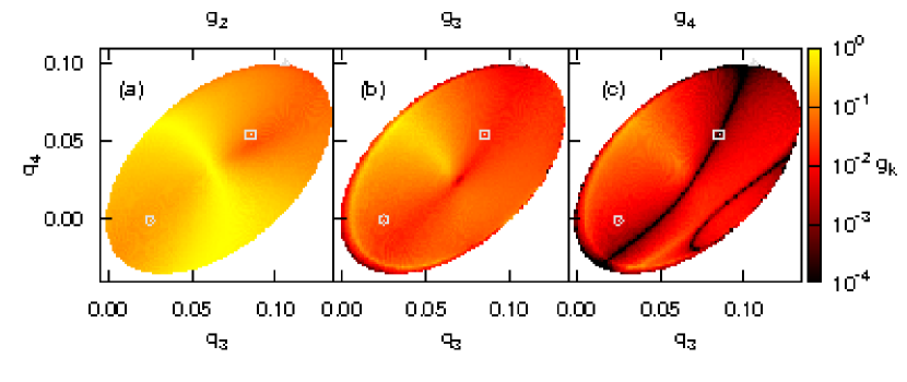
Figure 13: Regions of different $g_{k}$ (35) values for (a) $k=2$, (b) $k=3$, (c) $k=4$, in the subspace $(q_{3},q_{4})$ of the 4D Hamiltonian $H_{4}$ obtained from (6) for $N=4$ and $\beta=1.5$. The remaining coordinates of the considered initial conditions are set to $q_{1}=q_{2}=0.1$, $p_{1}=p_{2}=p_{3}=0$, while $p_{4}>0$ is evaluated so that $H_{4}=0.010075$. White regions correspond to forbidden initial conditions. The color scales shown at the right of the panels are used to color each point according to the orbit’s $g_{k}$ value at $t=10^{6}$. The points with coordinates $q_{3}=0.106$, $q_{4}=0.0996$ (marked by a triangle), $q_{3}=0.085109$, $q_{4}=0.054$ (marked by a square) and $q_{3}=0.025$, $q_{4}=0$ (marked by a circle) correspond to regular orbits on a 2d, a 3d and a 4d torus respectively (after GES_12 )

For this particular Hamiltonian we can have regular motion on 2d, 3d and 4d tori. Let us see now how we can exploit the results of Fig. 13 to locate such tori. Motion on 2d tori results in large final $g_{2}$ values and to small $g_{3}$ and $g_{4}$. So, such tori should be located in regions colored in yellow or light red in Fig. 13(a) and in black in Figs. 13(b) and (c). A region which satisfies these requirements is located at the upper border of the colored areas in Fig. 13. The evolution of the GALIs of an orbit with initial conditions in that region (denoted by a triangle in Fig. 13) is shown in Fig. 14(a) and it verifies that the motion takes place on a 2d torus, as only the GALI₂ remains constant.

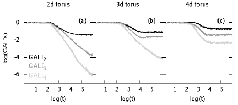
Figure 14: The time evolution of the GALI₂, the GALI₃ and the GALI₄ of regular orbits lying on a (a) 2d, (b) 3d, (c) 4d torus of the 4D Hamiltonian considered in Fig. 13. The initial conditions of these orbits are respectively marked by a triangle, a square and a circle in Fig. 13 (after GES_12 )

Extending the same argumentation to higher dimensions we see that motion on a 3d torus can occur in regions colored in yellow or light red in both Figs. 13(a) and (b) and in black in Fig. 13(c). The initial condition of an orbit of this kind is marked by a small square in Fig. 13. The evolution of this orbit’s GALIs (Fig. 14(b)) verifies that the orbit lies on a 3d torus, because only the GALI₂ and the GALI₃ remain constant. Orbits on 4d tori is the most common situation of regular motion for this 4D Hamiltonian system. This is evident from the results of Fig. 13 because most of the permitted area of initial conditions correspond to high $g_{2}$, $g_{3}$ and $g_{4}$ values. A randomly chosen initial condition in this region (marked by a circle in Fig. 13) results indeed to regular motion on a 4d torus as the constancy of its GALI_k, $k=2,3,4$ in Fig. 14(c) clearly indicates.

We note that initial conditions leading to chaotic motion in this system would correspond to very small $g_{2}$, $g_{3}$ and $g_{4}$ values (due to the exponential decay of the associated GALIs) and consequently would be colored in black in all panels of Fig. 13. The lack of such regions in Fig. 13 signifies that all considered initial conditions lead to regular motion. This happens because regions of chaotic motion occupy a tiny fraction of the system’s phase space, because its nonlinearity strength is very small. Therefore, chaotic motion is not captured by the grid of initial conditions of Fig. 13.

3.4 Behavior of the GALI for Periodic Orbits

Let us now discuss the behavior of the GALIs for periodic orbits of period $T$; i.e. orbits satisfying the condition $\vec{x}(t+T)=\vec{x}(t)$, with $\vec{x}(t)$ being the coordinate vector in the system’s phase space. In the presentation of this topic we mainly follow the analysis performed in MSA_12 . The linear stability of periodic orbits is defined by the eigenvalues of the so-called monodromy matrix, which is obtained by the solution of the variational equations (for Hamiltonian systems) or by the evolution of the tangent map (for symplectic maps) for one period $T$ (see for example B_69 ; S_01b and Sect. 3.3 of LL_92 ). When all eigenvalues lie on the unit circle in the complex plane the orbit is characterized as elliptic, while otherwise it is called hyperbolic (unstable). For a detailed presentation of the various stability types of periodic orbits the reader is referred for example to B_69 ; H_75 ; HM_87 ; HD_98 ; S_01b .

The presence of periodic orbits influence significantly the dynamics. In most systems we observe that the majority of non-periodic orbits in the vicinity of an elliptic one are regular. So, although initial conditions near an elliptic orbit can lead to chaos, regular orbits exhibiting a time evolution similar to the elliptic orbit itself prevail. If one assumes that the elliptic orbit is integrable and in its vicinity the Kolmogorov-Arnold-Moser (KAM) theorem (see for example Sect. 3.2 of LL_92 and references therein) can be applied (for which one needs to check a non-degeneracy condition which is typically satisfied), then there is large measure of orbits on KAM tori nearby. In Hamiltonian systems of dimension larger than 2 the phenomenon of Arnold diffusion (see for example Chap. 6 of LL_92 and references therein) typically would lead to an escape of orbits from the neighborhood of the elliptic orbit. However, it is generally believed that Arnold diffusion occurs on a slow time scale, and we do not expect interference with the GALI method. Of course, regular behavior on nearby KAM tori does not imply that the elliptic orbit itself is stable (e.g. Appendix of DMS00 ). On the other hand, in chaotic Hamiltonian systems and symplectic maps orbits in the vicinity of an unstable periodic orbit typically behave chaotically and diverge from the periodic one exponentially fast. This divergence is characterized by LEs (with at least one of them being positive) which are determined by the eigenvalues of the monodromy matrix (e.g. BFS_79 ; SBA_07 and Sect. 5.2b of LL_92 ). Thus, following arguments similar to the ones developed in Sect. 3.2 for chaotic orbits, we easily see that the GALI_k of unstable periodic orbits decreases to zero following the exponential law (22), i. e.

$$\mbox{GALI}_{k}(t)\propto\exp\left\{-\left[(\lambda_{1}-\lambda_{2})+(\lambda_{1}-\lambda_{3})+\cdots+(\lambda_{1}-\lambda_{k})\right]t\right\},$$ (36)

where $\lambda_{i}$, $i=1,\ldots,k$ are the periodic orbit’s $k$ largest LEs.

In Fig. 15(a) we see that the evolution of the GALIs for an unstable periodic orbit of the 2D Hamiltonian (4) is well approximated by (36) for $\lambda_{1}=0.084$. This value is the orbit’s mLE determined by the eigenvalues of the corresponding monodromy matrix (see MSA_12 for more details). We also note that according to (24) and (25) we set $\lambda_{1}=-\lambda_{4}$, and $\lambda_{2}=\lambda_{3}=0$ in (36). The agreement between the numerical data and the theoretical prediction (36) is lost after about $t\approx 350$ time units. This happens because the numerically computed orbit eventually deviates from the unstable periodic one due to unavoidable computational inaccuracies and enters the chaotic region around the periodic orbit. In general, this region is characterized by different LEs with respect to the ones of the periodic orbit. The effect of this behavior on the orbit’s finite time mLE $\Lambda_{1}$ (1) is seen in Fig. 15(b). The computed $\Lambda_{1}$ deviates from the value $\lambda_{1}=0.084$ (marked by a horizontal dotted line) at about the same time the GALI₂ changes its decreasing rate in Fig. 15(a). Eventually, $\Lambda_{1}$ stabilizes at another positive value, which characterizes the chaoticity of the region around the periodic orbit.

                 

Figure 15: The time evolution of (a) the GALI₂, the GALI₃, the GALI₄ and (b) the finite time mLE $\Lambda_{1}$ of an unstable periodic orbit of the 2D Hamiltonian (4) for $H_{2}=0.125$. The initial conditions of the orbit are $q_{1}=0$, $q_{2}=0.2083772012$, $p_{1}=0.4453146996$, $p_{2}=0.1196065752$. The straight lines in (a) correspond to functions proportional to $\exp(-\lambda_{1}t)$, $\exp(-2\lambda_{1}t)$ and $\exp(-4\lambda_{1}t)$, for $\lambda_{1}=0.084$, which is the mLE of the periodic orbit. The slope of each line is mentioned in the legend. The horizontal dotted line in (b) indicates the value $\lambda_{1}=0.084$ (after MSA_12 )

On the other hand, the case of stable periodic orbits is a bit more complicated, because the GALIs behave differently for Hamiltonian flows and symplectic maps. In MSA_12 it was shown analytically that for stable periodic orbits of $N$D Hamiltonian systems, with $N\geq 2$, the GALIs decay to zero following the following power laws

$$\mbox{GALI}_{k}(t)\propto\left\{\begin{array}[]{ll}\frac{1}{t^{k-1}}&\mbox{if $2\leq k\leq 2N-1$}\\ \frac{1}{t^{2N}}&\mbox{if $k=2N.$}\\ \end{array}\right.$$ (37)

We observe that this equation can be derived from (34), which describes the behavior of the GALIs for motion on an $s$d tori, by setting $s=1$. We note that the first branch of (34) is meaningless for $s=1$, while the other two branches take the forms appearing in (37). The connection between (34) and (37) is not surprising if we notice that a periodic orbit is nothing more than an 1d closed curve in the system’s phase space, having the some dimension with an 1d torus.

Small, random perturbations from the stable periodic orbit generally results in regular motion on an $N$d torus. So, the GALIs of the perturbed orbit will follow (23). Thus, in general, the GALIs of regular orbits in the vicinity of a stable periodic orbit behave differently with respect to the indices of the periodic orbit itself (except from the GALI_2N and the GALI_2N-1, which respectively follow the laws $\propto t^{-2N}$ and $\propto t^{-(2N-2)}$ in both cases). The most profound change happens for the GALIs of order $2\leq k\leq N$ because, according to (23), they remain constant in the neighborhood of the periodic orbit, while they decay to zero following the power law (37) for the periodic orbit.

The correctness of (37) becomes evident from the results of Fig. 16(a), where the time evolution of the GALIs of a stable periodic orbit of the 2D Hamiltonian (4) is shown. In particular, we see that the indices decay to zero following the power laws GALI${}_{2}\propto t^{-1}$, GALI${}_{3}\propto t^{-2}$, GALI${}_{4}\propto t^{-4}$ predicted from (37). According to (23) the GALIs of regular orbits in the neighborhood of the stable periodic orbit should behave as GALI${}_{2}\propto\mbox{constant}$, GALI${}_{3}\propto t^{-2}$ and GALI${}_{4}\propto t^{-4}$. Thus, only the GALI₂ is expected to behave differently for regular orbits in the vicinity of the periodic orbit of Fig. 16(a). The results of Fig. 16(b) show that this is actually true. The GALI₂ of the neighboring regular orbits initially follows the same power law decay of the periodic orbit (GALI${}_{2}\propto t^{-1}$), but later on it stabilizes to a constant positive value. We see that the further the orbit is located from the periodic one the sooner the GALI₂ deviates from the power law decay.

                  

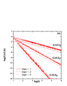
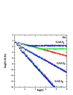
Figure 16: (a) The time evolution of the GALI₂, the GALI₃ and the GALI₄ for a stable periodic orbit of the 2D Hamiltonian (4) for $H_{2}=0.125$. The orbit’s initial conditions are $q_{1}=0=q_{10}$, $q_{2}=0.35207=q_{20}$, $p_{1}=0.36427=p_{10}$, $p_{2}=0.14979=p_{20}$. The straight lines correspond to functions proportional to $t^{-1}$, $t^{-2}$ and $t^{-4}$. The slope of each line is mentioned in the legend. (b) The same plot as in (a) where apart from the GALIs of the stable periodic orbit (red curves) the indices of two neighboring, regular orbits are also plotted. Their initial conditions are $q_{1}=q_{10}$, $p_{2}=p_{20}$ for both of them, while $q_{2}=q_{20}+0.00793$ (green curves), and $q_{2}=q_{20}+0.02793$ (blue curves). In both cases the $p_{1}>0$ initial condition is set so that $H_{2}=0.125$. Note that the curves of the GALI₃ and the GALI₄ for all three orbits overlap each other (after MSA_12 )

These differences of the GALI₂ values can be used to identify the location of stable periodic orbits in the system’s phase space, although the index was not developed for this particular purpose This becomes evident from the result of Fig. 17 where the values of the GALI₂ at $t=10^{5}$ for several orbits of the Hénon-Heiles system (4) are plotted as a function of the $q_{2}$ coordinate of the orbits’ initial conditions. The remaining coordinates are $q_{1}=p_{2}=0$, while $p_{1}>0$ is set so that $H_{2}=0.125$. Actually these initial conditions lie on the symmetry line of the subspace defined by $q_{1}=0$, $p_{1}>0$, i.e. the horizontal line $p_{2}=0$ in Figs. 19 and 20 below. This line passes through the initial condition of some periodic orbits of the system. For the construction of Fig. 17 we considered an ensemble of $7\,000$ orbits whose $q_{2}$ coordinates are equally distributed in the interval $-0.1\leq q_{2}\leq 0.6$. The data points are line connected, so that the changes of the GALI₂ values become easily visible.

t]

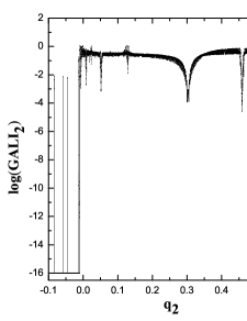
Figure 17: The values of the GALI₂ at $t=10^{5}$ for several orbits of the 2D Hamiltonian (4) as a function of the $q_{2}$ coordinate of the orbits’ initial conditions. The remaining coordinates are $q_{1}=p_{2}=0$, while $p_{1}>0$ is set so that $H_{2}=0.125$. Actually these initial conditions lie on the $p_{2}=0$ line of Figs. 19 and 20. The numerical data (black points) are line connected (grey line) in order to facilitate the visualization of the value changes (after MSA_12 )

In Fig. 17 regions of relatively large GALI₂ values ($\gtrsim 10^{-4}$) correspond to regular (periodic or quasiperiodic) motion. Chaotic orbits and unstable periodic orbits have very small GALI₂ values ($\lesssim 10^{-12}$), while domains with intermediate values ($10^{-12}\lesssim\mbox{GALI}_{2}\lesssim 10^{-4}$) correspond to sticky chaotic orbits. An interesting feature of Fig. 17 is the appearance of some relatively narrow regions where the GALI₂ decreases abruptly obtaining values $10^{-4}\lesssim\mbox{GALI}_{2}\lesssim 10^{-1}$; the most profound one being in the vicinity of $q_{2}\approx 0.3$. These regions correspond to the immediate neighborhoods of stable periodic orbits, with the periodic orbit itself been located at the point with the smallest GALI₂ value.

The creation of these characteristic ‘pointy’ shapes is due to the behavior depicted in Fig. 16(b): the GALI₂ has relatively small values on the stable periodic orbit, for which it decreases as $\propto t^{-1}$, while it attains constant, positive values for regular orbits in the vicinity of the periodic orbit. These constant values increase as the orbit’s initial conditions depart further away from the periodic orbit. So, more generally, the appearance of such ‘pointy’ formations in GALI_k plots ($2\leq k\leq N$) provide good indications for the location of stable periodic orbits.

Let us now turn our attention to maps. In $2N$d symplectic maps stable periodic orbits of period $l$ correspond to $l$ distinct points (the so-called stable fixed points of order $l$). Any deviation vector from the periodic orbit rotates around each fixed point. This behavior can be easily seen in the case of 2d maps where the tori around a stable fixed point correspond to closed invariant curves which can be represented, through linearization, by ellipses (see for example Sect. 3.3b of LL_92 ). Thus, any $k$ initially distinct deviation vectors needed for the computation of the GALI_k will rotate around the fixed point keeping on average the angles between them constant. Consequently the volume of the parallelepiped they define, i.e. the value of the GALI_k, will remain practically constant. Thus, in the case of stable periodic orbits of $2N$d maps, with $N\geq 1$ we have

$$\mbox{GALI}_{k}(t)\propto\mbox{constant},\,\,\,\,\mbox{ for $2\leq k\leq 2N$}.$$ (38)

This behavior is clearly seen in Fig. 18(a) where the evolution of the GALI₂, the GALI₃ and the GALI₄ for a stable periodic orbit of period 7 of the 4d map (30) is plotted.

                  

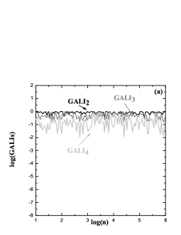
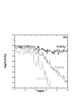
Figure 18: The evolution of the GALI₂, the GALI₃ and the GALI₄ with respect to the number of iterations $n$ for (a) a stable periodic orbit and (b) a nearby regular orbit, of the 4d map (30) with $K=0.9$ and $\gamma=0.05$. The initial conditions of the orbits are: (a) $x_{1}=0.23666$, $y_{1}=0.0$, $x_{2}=0.23666$, $y_{2}=0.0$, and (b) $x_{1}=0.23$, $y_{1}=0.0$, $x_{2}=0.236$, $y_{2}=0.0$

Again small perturbations of the periodic orbit’s initial conditions generally result in motion on an $N$d tori. Then, the evolution of the corresponding GALIs is provided by (23) for $N\geq 2$, while the GALI₂ will decrease to zero according to (33) for 2d maps. So, the most striking difference between the behavior of the GALI_k of a stable periodic orbit and of a neighboring, regular orbit appears for $k>N$, because in this case the GALI_k remains constant for the periodic orbit, while it decays to zero for the neighboring one. Differences of this kind can be observed in Fig.18(b).

4 Applications

The ability of the SALI and the GALI methods to efficiently discriminate between chaotic and regular motion was described in detail in the previous sections, where some exemplary Hamiltonian systems and symplectic maps were considered. In what follows we present applications of this ability to various dynamical systems originating from different research fields.

4.1 Global Dynamics

In Sect. 3.2 we discussed how one can use the various GALIs to reveal the chaotic or regular nature of individual orbits in the $2N$d phase space of a dynamical system. Additionally, in Sect. 3.4 we saw how the measurement of the GALI₂ values for an ensemble of orbits can facilitate the uncovering of some dynamical properties of the studied system, in particular the pinpointing of stable periodic orbits (Fig. 17), while in Sect. 3.3 we described how a more general search can help us locate motion on low dimensional tori.

Now we see how one can use the GALIs in order to study the global dynamics of a system. For simplicity we use in our analysis the 2D Hamiltonian system (4), but the methods presented below can be (and actually have already been) implemented to higher-dimensional systems.

Investigating Global Dynamics by the GALI_k with $2\leq k\leq N$

According to (22) and (23) the GALI_k, with $2\leq k\leq N$, behaves in a completely different way for chaotic (exponential decay) and regular (remains practically constant) orbits. Thus, by coloring each initial condition of an ensemble of orbits according to its GALI_k value at the end of a fixed integration time we can produce color plots where regions of chaotic and regular motion are easily seen. In addition, by choosing an appropriate threshold value for the GALI_k, below which the orbit is characterized as chaotic (see Sect. 3.2 on how to set up this threshold), we can efficiently determine the ‘strength’ of chaos by calculating the percentage of chaotic orbits in the studied ensemble. Then, by performing the same analysis for different parameter values of the system we can determine its physical mechanisms that increase or suppress chaotic behavior.

A practical question arises though: which index should one use for this kind of analysis? The obvious advantage of the GALI₂/SALI is its easy computation according to (8), which requires the evolution of only two deviation vectors. On the other hand, evaluating the GALIs of order up to $k=N$ is more CPU-time consuming as the computation of the index from (20) requires the evolution of more deviation vectors, as well as the implementation of the SVD algorithm. An advantage of these higher order indices is that they tend to zero faster than the GALI₂/SALI for chaotic orbits. So, reaching their threshold value which characterizes an orbit as chaotic, requires in general, less computational effort. This feature is particularly useful when we want to estimate the percentage of chaotic orbits, as there is no need to continue integrating orbits which have been characterized as chaotic (see Sect. 5.2 of SBA_07 for an example of this kind). Thus, we conclude that the reasonable choices for such global studies are the GALI₂/SALI and the GALI_N.

In order to illustrate this process, let us consider the 2D Hénon-Heiles system (4), for which $\mbox{GALI}_{N}\,\equiv\,\mbox{GALI}_{2}$, since $N=2$. In Fig. 19 we see color plots of its Poincaré surface of section defined by $q_{1}=0$ (a concise description of the construction of a surface of section can be found for instance in Sect. 1.2b of LL_92 ). The remaining initial conditions of each orbit are its coordinates on the $(q_{2},p_{2})$ plane of Fig. 19, while $p_{1}>0$ is set so that $H_{2}=0.125$. For each panel of Fig. 19 a 2d grid of approximately $350\,000$ equally distributed initial conditions is considered. Each point on the $(q_{2},p_{2})$ plane is colored according to its $\log(\mbox{GALI}_{2})$ value at $t=2\,000$, while white regions denote not permitted initial conditions. Regions colored in yellow or light red correspond to regular orbits, while dark blue and black domains contain chaotic ones. Intermediate colors at the borders between these two regions indicate sticky chaotic orbits.

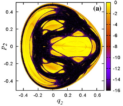
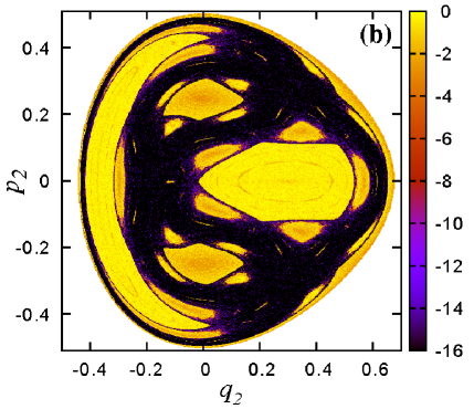
Figure 19: Regions of different values of the GALI₂ on the Poincaré surface of section defined by $q_{1}=0$ of the 2D Hamiltonian (4) for $H_{2}$=0.125. A set of approximately $350\,000$ equally spaced initial conditions on the grid $(q_{2},p_{2})\in[-0.5,0.7]\times[-0.5,0.5]$ is used. White regions correspond to forbidden initial conditions. The color scales shown at the right of the panels are used to color each point according to the orbit’s $\log(\mbox{GALI}_{2})$ value at $t=2\,000$. In (a) the same set of initial orthonormal deviation vectors was used for the computation of the GALI₂ of each initial condition, while in (b) a different, randomly produced set of vectors was used for each orbit

This kind of color plots can reveal fine details of the underlying dynamics, like for example the small yellow ‘islands’ of regular motion inside the large, black chaotic ‘sea’, as well as allow the accurate estimation of the percentage of chaotic or regular orbits in the studied ensemble. Naturally the denser the used grid is, the finer the uncovered details become, but unfortunately the higher the needed computational effort gets. In an attempt to speed up the whole process the following procedure was followed in AMS_05 where the dynamics of the Hénon-Heiles system (4) was studied. The final GALI₂/SALI value and the corresponding color was assigned not only to the initial condition of the studied orbit, but also to all intersection points of the orbit with the surface of section. This assignment can be extended even further by additionally taking into account the symmetry of Hamiltonian (4) with respect to the $q_{2}$ variable, which results in structures symmetric with respect to the $p_{2}=0$ axis in Fig. 19. Consequently, points symmetric to this axis should have the same GALI₂/SALI value. So, orbits with initial conditions on grid points to which a color has already been assigned, as they were intersection points with the surface of section of previously computed orbits, are not computed again and so the construction of color plots like the ones of Fig. 19 is speeded up significantly. In AMS_05 it was shown that this approach achieves very accurate estimations of the percentages of chaotic orbits with respect to the ones obtaining by coloring each and every initial condition according to the index’s value at the end of the integration time (this is actually how Fig. 19 was produced).

Let us now discuss the differences between panels (a) and (b) of Fig. 19. In both figures the chaotic regions are practically the same. Nevertheless, in the yellow and light red colored domains, where regular motion occurs, some ‘spurious’ structures appear in Fig. 19(a), which are not present in Fig. 19(b). For example, inside the large stability island with $0\lesssim q_{2}\lesssim 0.5$ at the right side of Fig. 19(a) we observe an almost horizontal formation colored in light red, while similar colored ‘arcs’ appear inside many other islands of regular motion. These artificial features emerge when one uses exactly the same set of orthonormal, initial deviation vectors for every studied orbit, as we did in Fig. 19(a). The appearance of such features in color plots of other chaos detection methods has already been reported in the literature BBB_09 . A simple way to avoid them is to use a different, random set of initial, orthonormal vectors for the computation of the GALI₂, as we did in Fig. 19(b). By doing so, these spurious features disappear and only structures related to the actual dynamics of the system remain, like for instance the cyclical ‘chain’ of the light red colored, elongated regions inside the big stability island at the right side of Fig. 19(b). This structure indicates the existence of some higher order stability island, which are surrounded by an extremely thin chaotic layer. This layer is not visible for the resolution used in Fig. 19(b). A magnification, and a much finer grid would reveal this tiny chaotic region.

Investigating Global Dynamics by the GALI_k with $N<k\leq 2N$

As was clearly explained in Sect. 3.2 the GALIs of order $N<k\leq 2N$ tend to zero both for chaotic and regular orbits, but with very different time rates as (22) and (23) state. This deference can be also used to investigate global dynamics, but following an alternative approach to the one developed in Sect. 4.1. Since these GALIs decay to zero exponentially fast for chaotic orbits, but follow a much slower power law decay for regular ones, the time $t_{th}$ they need to reach an appropriately chosen, small threshold value will be significantly different for the two kinds of orbits. We note that both the exponential and the power law decays become faster with increasing order $k$ of GALI_k. Consequently, the creation of huge differences in the GALI_k values, which allow the discrimination between chaotic and regular motion, will appear earlier for larger $k$ values. So, in general, the overall required computational time decreases significantly by using a higher order GALI_k, despite the integration of more deviation vectors, since this integration will be terminated earlier. Thus, the best choice in investigations of this kind is to use the GALI_2N.

Let us illustrate this approach by computing the GALI₄ for the 2D Hénon-Heiles system (4), at a grid in its $q_{1}=0$ surface of section. The outcome of this procedure is seen in Fig. 20, where each initial condition is colored according to the time $t_{th}$ needed for its GALI₄ to become $\leq 10^{-12}$. Each orbit is integrated up to $t=500$ time units and if its GALI₄ value at the end of the integration is larger than the threshold value $10^{-12}$ the corresponding $t_{th}$ value is set to $t_{th}=500$ and the initial condition is colored in blue according to the color scales seen below the panel of Fig. 20. Regions of regular motion correspond to large $t_{th}$ values and are colored in blue, while all the remaining colored domains contain chaotic orbits. Again, white regions correspond to forbidden initial conditions. This approach yields a very detailed chart of the dynamics, analogous to the one seen in Fig. 19.

t]

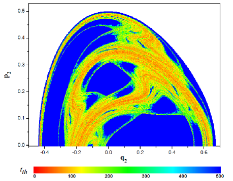
Figure 20: Regions of different values of the time $t_{th}$ needed for the GALI₄ to become less than $10^{-12}$ on the $q_{1}=0$ surface of section of the 2D Hénon-Heiles system (4). Each orbit is integrated up to $t=500$ time units. White regions correspond to forbidden initial conditions. The color scales shown below the panel are used to color each point according to the orbit’s $t_{th}$ value (after SBA_07 )

An advantage of the current approach is its ability to clearly reveal various ‘degrees’ of chaotic behavior in regions not colored in blue. Strongly chaotic orbits are colored in red and yellow as their GALI₄ becomes $\leq 10^{-12}$ quite fast. Orbits with larger $t_{th}$ values correspond to chaotic orbits which need more time in order to show their chaotic nature, while the ‘sticky’ chaotic regions are characterized by even higher $t_{th}$ values and are colored in light blue. We note that for every initial condition we used a different, random set of orthonormal deviation vectors in order to avoid the appearance of possible ‘spurious’ structures, like the ones seen in Fig. 19(a).

4.2 Studies of Various Dynamical Systems

The SALI and the GALI methods have been used broadly for the study of the phase space dynamics of several models originating from different scientific fields. These studies include the characterization of individual orbits as chaotic or regular, as well as the consideration of large ensembles of initial conditions along the lines presented in Sect. 4.1, whenever a more global understanding of the underlying dynamics was needed.

In this section we present a brief, qualitative overview of such investigations. For this purpose we focus mainly on the outcomes of these studies avoiding a detailed presentation of mathematical formulas and equations for each studied model.

An Accelerator Map Model

Initially, let us discuss two representative applications of the SALI. The first one concerns the study of a 4d symplectic map which describes the evolution of a charged particle in an accelerator ring having a localized thin sextupole magnet. The specific form of this map can be found in BS_06 where the SALI method was used for the construction of phase space color charts where regions of chaotic and regular motion were clearly identified, as well as for evaluating the percentage of chaotic orbits.

Later on, in BCSV_12 ; BCSPV_12 this map was used to test the efficiency of chaos control techniques for increasing the stability domain (the so-called ‘dynamic aperture’) around the ideal circular orbit of this simplified accelerator model. These techniques turned out to be quite successful, as the addition of a rather simple control term, which potentially could be approximated by real multipole magnets, increased the the stability region of the map as can be seen in Fig. 21.

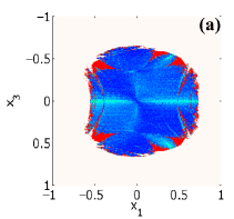
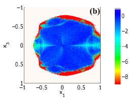
Figure 21: Regions of different SALI values of (a) the 4d uncontrolled accelerator map studied in BS_06 and (b) the controlled map constructed in BCSV_12 . The coordinates $x_{1}$, $x_{3}$ respectively describe horizontal and vertical deflections of a charged particle from the ideal circular orbit passing from $x_{1}=x_{3}=0$ in some appropriate units (see BS_06 for more details). $16\,000$ uniformly distributed initial conditions on the grid $(x_{1},x_{3})\in[-1,1]\times[-1,1]$ were evolved for $10^{5}$ iterations of each map and colored according to the orbit’s $\log(\mbox{SALI})$ value, using the color scales shown at the right of the panels. The white colored regions correspond to orbits that escape in less than $10^{5}$ iterations. Red points denote chaotic orbits, while regular ones are colored in blue. The increase of the stability region around the point $x_{1}=x_{3}=0$ is evident (after BCSPV_12 )

A Hamiltonian Model of a Bose-Einstein condensate

Let us now turn our attention to a 2D Hamiltonian system describing the interaction of three vortices in an atomic Bose-Einstein condensate, which was studied in KKSK_14 . By means of SALI color plots the extent of chaos in this model was accurately measured and its dependence on physically important parameters, like the energy and the angular momentum of the vortices, were determined.

In real experiments, from which the study of this model was motivated, the life time of Bose-Einstein condensates is limited. For this reason the time in which the chaotic nature of orbits is uncovered played a significant role in the analysis presented in KKSK_14 . Actually, different ‘degrees of chaoticity’ are revealed by registering the time $t_{th}$ that the SALI of a chaotic orbit requires in order to become $\leq 10^{-12}$ (Fig. 22). This approach is similar to the one presented in Sect. 4.1, and allows the identification of regions with different strengths of chaos.

 

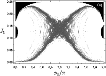
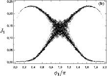
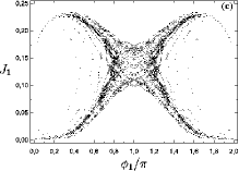
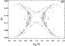
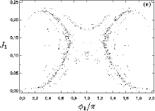
Figure 22: (a) Regions of different values of the time $t_{th}$ needed for the SALI to become less than $10^{-12}$ for a 2D Hamiltonian describing the interaction of three vortices in an atomic Bose-Einstein condensate. The explicit definition of the coordinates $J_{1}$ and $\phi_{1}/\pi$ can be found in KKSK_14 where this model was studied in detail. Each orbit is integrated up to $t=3\,000$ time units. White regions correspond to regular orbits, while black areas at the upper two corners, as well as in the middle of the vertical axes at both sides of the plot, denote not permitted initial conditions. The color scales shown at the right of the panel are used to color each point according to the orbit’s $t_{th}$ value. The initial conditions of (a) are decomposed in four different sets according to their $t_{th}$ value: (b) $140\leq t_{th}\leq 500$, (c) $500<t_{th}\leq 1\,000$, (d) $1\,000<t_{th}\leq 1\,500$ and (e) $1\,500<t_{th}\leq 2\,000$ (after KKSK_14 )

The chaotic orbits of Fig. 22(a) are decomposed in Figs. 22(b)–(e) in four different sets according to their $t_{th}$ value: $t_{th}\in[140,500]$ (Fig. 22(b)), $t_{th}\in(500,1\,000]$ (Fig. 22(c)), $t_{th}\in(1\,000,1\,500]$ (Fig. 22(d)) and $t_{th}\in(1\,500,2\,000]$ (Fig. 22(e)), where time is measured in some appropriate units (see KKSK_14 for more details). From these results we see that, as the initial conditions move further away from the center of the x-shaped region of Fig. 22(a) the orbits need more time to show their chaotic nature and consequently, some of them can be considered as regular from a practical (experimental) point of view. For instance, in real experiments one would expect to detect chaotic motion in regions shown in Fig. 22(b) where orbits have relatively small $t_{th}$ values. Thus, an analysis of this kind can provide practical information about where one should look for chaotic behavior in actual experimental set ups.

Further Applications of the SALI and the GALI Methods

The SALI and the GALI methods have been successfully employed in studies of various physical problems and mathematical toy models, as well as for the investigation of fundamental aspects of nonlinear dynamics (e.g. see CEGM_14 ). In what follows we briefly present some of these studies

In MSAB2008 the SALI/GALI₂ method was used for the global study of the standard map (32). By considering large ensembles of initial conditions the percentage of chaotic motion was accurately computed as a function of the map’s parameter $K$. This work revealed the periodic re-appearance of small (even tiny) islands of stability in the system’s phase space for increasing values of $K$. Subsequent investigations of the regular motion of the standard map in ManRob2014 led to the clear distinction between typical islands of stability and the so-called accelerator modes, i.e. motion resulting in an anomalous enhancement of the linear in time orbits’ diffusion. Typically, this motion is highly superdiffusive and is characterized by a diffusion exponent $\approx 2$.

In BMC2009 the GALI was used for the detection of chaotic orbits in many dimensions, the prediction of slow diffusion, as well as the determination of quasiperiodic motion on low dimensional tori in the system (7) of many coupled standard maps. Additional applications of the SALI in studying maps can be found in PABV2008 , where the index was used for shedding some light in the properties of accelerator models, while in SS2012 a coupled logistic type predator-prey model describing population growths in biological systems was considered. Further studies of 2d and 4d maps based on the SALI method were performed in FMT2012 .

Models of dynamical astronomy and galactic dynamics are considered to be the spearhead of the chaos detection methods Cont_book . Actually, many of these methods have been used, or often even constructed, to investigate the properties of such systems. Several applications of the SALI to systems of this kind can be found in the literature. In SBD2007 ; SPB2008 ; BP2009 the stability properties of orbits in a particular few-body problem, the so-called the Sitnikov problem, were studied, while in Voy2008 the long term stability of two-planet extrasolar systems initially trapped in the 3:1 mean motion resonance was investigated. The SALI was also used to study the dynamics of the Caledonian symmetric four-body problem SESS2013 , as well as the circular restricted three-body problem R_14 .

In systems modeling the dynamics of galaxies special care should be taken with respect to the determination of the star motion’s nature, because this has to be done as fast as possible and in physically relevant time intervals (e.g. smaller than the age of the universe). Hence, in order to check the adequacy of a proposed galactic model, in terms of being able to sustain structures resembling the ones seen in observations of real galaxies, the detection of chaotic and regular motion for rather small integration times is imperative. The SALI and the GALI methods have proved to be quite efficient tools for such studies, as they allow the fast characterization of orbits. This ability reduces significantly the required computational burden, as in many cases the determination of the orbits’ nature is achieved before the predefined, final integration time.

In particular, the SALI method has been used successfully in studying the chaotic motion and spiral structure in self-consistent models of rotating galaxies VHC2007 , the dynamics of self-consistent models of cuspy triaxial galaxies with dark matter haloes CDLMV2007 , the orbital structure in $N$ body models of barred-spiral galaxies HK2009 , the secular evolution of elliptical galaxies with central masses K2008 , the chaotic component of cuspy triaxial stellar systems CMN_14 , as well as the chaoticity of non-axially symmetric galactic models ZotCar2013 and of models with different types of dark matter halo components Zot2014 .

The SALI was used in MSAB2008 for investigating the dynamics of 2D and 3D Hamiltonian models of rotating bared galaxies. This work was extended in MA2011 by using the GALI for studying the global dynamics of different galactic models of this type. In particular, the effects of several parameters related to the shape and the mass of the disk, the bulge and the bar components of the models, as well as the rotation speed of the bar, on the amount of chaos appearing in the system were determined. Moreover, the implementation of the GALI₃ in the 3D Hamiltonians allowed the detection of regular motion on low (2d) dimensional tori, although these systems support, in general, 3d orbits. The astronomical significance of these orbits was discussed in detail in MA2011 .

Implementations of the SALI to nuclear physics systems can be found in SCM2007 ; MSCHJD2007 ; SHC2009 ; MDSC2010 ; MDC2010 where the chaotic behavior of boson models is investigated, as well as in ABB2010 where the dynamics of a Hamiltonian model describing a confined microplasma was studied. Recently the SALI and the GALI methods, together with other chaos indicators, were reformulated in the framework of general relativity, in order to become invariant under coordinate transformation Luk2014 .

The SALI and the GALI have been also used to study the dynamics of nonlinear lattice models. Applications of these indices to the Fermi-Pasta-Ulam model can be found in AB2006 ; CB2006 ; ABS_06 ; SBA_08 ; PP2008 ; CEB2010 ; AC2011 ; CE2013 where the properties of regular motion on low dimensional tori, the long term stability of orbits, as well as the interpretation of Fermi-Pasta-Ulam recurrences were studied. In ManRuf2011 the GALI method managed to capture the appearance of a second order phase transition that the Hamiltonian Mean Field model exhibits at a certain energy density. The index successfully verified also other characteristics of the system, like the sharp transition from weak to strong chaos. Further applications of the SALI method to other models of nonlinear lattices can be found in PBS_04 ; ABS_06 .

In addition, the SALI was further used in studying the chaotic and regular nature of orbits in non-Hamiltonian dynamical systems HuaWu2011 ; ABDNT2013 , some of which model chaotic electronic circuits HuaWu2012 ; HuaZhou2013 ; HuaCao2014 .

4.3 Time Dependent Hamiltonians

The applications presented so far concerned autonomous dynamical systems. However, there are several phenomena in nature whose modeling requires the invocation of parameters that vary in time. Whenever these phenomena are described according to the Hamiltonian formalism, the corresponding Hamiltonian function is not an integral of motion as its value does not remain constant as time evolves.

The SALI and the GALI methods can be also used to determine the chaotic or regular nature of orbits in time dependent systems as long as, their phase space does not shrink ceaseless or expand unlimited, with respect to its initial volume, during the considered times. This property allows us to utilize the time evolution of the volume defined by the deviation vectors, as in the case of the time independent models, and estimate accurately its possible decay for time intervals where the total phase space volume has not changed significantly.

In conservative time independent Hamiltonians orbits can be periodic (stable or unstable), regular (quasiperiodic) or chaotic and their nature does not change in time. Sticky chaotic orbits may exhibit a change in their orbital morphologies from almost quasiperiodic to completely chaotic behaviors, but in reality their nature does not change as they are weakly chaotic orbits. On the other hand, in time dependent models, individual orbits can display abrupt transitions from regular to chaotic behavior, and vice versa, during their time evolution. This is an intriguing characteristic of these systems which should be captured by the used chaos indicator. Such transitions between chaotic and regular behaviors can be seen for example in $N$ body simulations of galactic models. For this reason, time dependent analytic potentials trying to mimic the evolution of $N$ body galactic systems, are expected to exhibit similar transitions.

An analytic time dependent bared galaxy model consisting of a bar, a disk and a bulge component, whose masses vary linearly in time was studied in MBS2013 . The time dependent nature of the model influences drastically the location and the size of stability islands in the system’s phase space, leading to a continuous interplay between chaotic and regular behaviors. The GALI was able to capture subtle changes in the nature of individual orbits (or ensemble of orbits) even for relatively small time intervals, verifying that it is an ideal diagnostic tool for detecting dynamical transitions in time dependent systems.

Although both 2D and 3D time dependent Hamiltonian models were studied in MBS2013 , we further discuss here only the 3D model in order to illustrate the procedure followed for detecting the various dynamical epochs in the evolution of an orbit. The main idea for doing that is the re-initialization of the computation of the GALI_k, with $2\leq k\leq N$, whenever the index reaches a predefined low value (which signifies chaotic behavior) by considering $k$ new, orthonormal deviation vectors resetting GALI${}_{k}=1$.

Let us see this procedure in more detail. In MBS2013 the evolution of the GALI₃ was followed for each studied orbit. The three randomly chosen, initial deviations vectors set GALI${}_{3}=1$ in the beginning of the numerical simulation (t=0). These vectors were evolved according to the dynamics induced by the 3D, time dependent Hamiltonian up to the time $t=t_{d}$ that the GALI₃ became smaller than $10^{-8}$ for the fist time. At that point the time $t=t_{d}$ was registered and three new, random, orthonormal vectors were considered resetting GALI${}_{3}=1$. Afterwards, the evolution of these vectors was followed until the next, possible occurrence of GALI${}_{3}<10^{-8}$. Then the same process was repeated.

Why was this procedure implemented? What is the reason behind this strategy? In order to reveal this reason let us assume that an orbit initially behaves in a chaotic way and later on it drifts to a regular behavior. The volume formed by the deviation vectors will shrink exponentially fast, becoming very small during the initial chaotic epoch and will remain small throughout the whole evolution in the regular epoch, unless one re-initializes the deviation vectors and the volume they define. In this way the deviation vectors will be able to ‘feel’ the new, current dynamics.

An example case of this kind is shown in Fig. 23. In particular, in Fig. 23(a) we see that the evolution of the finite time mLE $\Lambda_{1}$ is not able to provide valid information about the different dynamical epochs that the studied orbit experiences. This is due to the index’s averaging nature which takes into account the whole history of the evolution. On the other hand, the re-initialized GALI₃ (whose time evolution is shown in Fig. 23(b)) clearly succeeds in depicting the transitions between regular epochs, where it oscillates around positive values (such time intervals are denoted by I and III in Figs. 23(a) and (b)), and chaotic ones, where it exhibits repeated exponential decays to very small values (epoch II). From the results of Fig. 23(a) it becomes evident that the computation of the mLE cannot be used as a reliable criterion for determining the chaotic or regular nature of the orbit in these three time intervals.

 

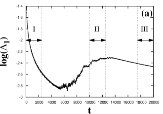
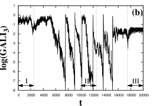
Figure 23: Time evolution of (a) the finite time mLE $\Lambda_{1}$, (b) the re-initialized GALI₃, and (c) the time $t_{d}$ needed for the re-initialized GALI₃ to decrease from GALI${}_{3}=1$ to GALI${}_{3}\leq 10^{-8}$ for a particular orbit of the 3D time dependent galactic model studied in MBS2013 . The orbit changes its dynamical nature from regular to chaotic and again to regular. Three characteristic epochs are located between the vertical dashed gray lines in (a) and (b) and are denoted by I (regular), II (chaotic) and III (regular). The arrow at the right end of (c) indicates that after $t\gtrsim 15000$ the GALI₃ in (b) does not fall back to zero (until of course, the final integration time $t=20\,000$), which is a clear indication that in this time interval the orbit is regular (after MBS2013 )

Another way to visualize the results of Fig. 23(b) is through the measurement of the time $t_{d}$ needed for the repeated re-initializations of the GALI₃, or in other words, of the time needed for the GALI₃ to decrease from GALI${}_{3}=1$ to GALI${}_{3}\leq 10^{-8}$. In Fig. 23(c) we present $t_{d}$ as a function of the evolution time of the orbit. From the results of this figure we see that during the time interval $7500\lesssim t\lesssim 14000$ the value of $t_{d}$ is rather small, indicating strong chaotic motion. For smaller times, $t\lesssim 7500$, the GALI₃ takes a long time to become small, suggesting the presence of regular motion or of (relatively) weaker chaotic motion. The upwardly pointing arrow, after $t\gtrsim 15000$, shows that the GALI₃ no longer falls to zero, which again indicates the appearance of a regular epoch.

After the first, successful application of the GALIs to time dependent Hamiltonians in MBS2013 , the same approach was followed for the study of a more sophisticated time dependent galactic model in ManMach2014 . This analytic Hamiltonian model succeeded to incorporate the evolution of the basic morphological features of an actual $N$ body simulation, by allowing all the relevant parameters of its dynamical components to vary in time.

5 Summary

In this chapter we presented how the SALI and the various GALIs can be used to study the chaotic behavior of dynamical systems.

Following the history of the evolution of these indices, we initially presented in Sect. 2 the underlying idea behind the introduction of the SALI: the index actually quantifies the possible alignment of two initially distinct deviation vectors. The natural generalization of this idea, by considering more than two deviation vectors and checking if they become linearly dependent, led later on, to the introduction of the GALI, as we explained in Sect. 3. The close relation between the two indices was also pointed out, as according to (17) the GALI₂ and the SALI practically coincide

$$\mbox{GALI}_{2}\propto\mbox{SALI}.$$

Avoiding the presentation of mathematical proofs (which the interested reader can find in the related references), we formulated in Sect. 3 the laws that the indices follow for chaotic and regular orbits, providing also several numerical results which demonstrate their validity.

In particular, for $N$D Hamiltonian systems ($N\geq 2$) and $2N$d symplectic maps ($N\geq 1$) the GALI_k tends exponentially to zero for chaotic orbits and unstable periodic orbits following (22)

$$\mbox{GALI}_{k}(t)\propto\exp\left\{-\left[(\lambda_{1}-\lambda_{2})+(\lambda_{1}-\lambda_{3})+\cdots+(\lambda_{1}-\lambda_{k})\right]t\right\},$$

while for regular motion on as $s$d torus, with $2\leq s\leq N$, the evolution of the GALI_k is given by (34)

$$\mbox{GALI}_{k}(t)\propto\left\{\begin{array}[]{ll}\mbox{constant}&\mbox{if $2\leq k\leq s$}\\ \frac{1}{t^{k-s}}&\mbox{if $s<k\leq 2N-s$}\\ \frac{1}{t^{2(k-N)}}&\mbox{if $2N-s<k\leq 2N.$}\\ \end{array}\right.$$

The latter formula is quite general as a) for $s=N$ it provides (23), which describes the behavior of the GALI_k for motion on an $N$d torus, i.e. the most common situation of regular motion in the $2N$d phase space of the system, b) for $k=2$, $s=1$ and $N=1$ it gives (33), which describes the power law decay of the GALI₂ in the case of a 2d map (the GALI₂ is only possible GALI in this case), and c) for $s=1$ it becomes (37), which provides the power law decay of the GALI_k for stable periodic orbits of Hamiltonian systems (we remind that in the case of stable periodic in maps all the GALIs remain constant (38)).

In our presentation, we paid much attention to issues concerning the actual computation of the indices. In Sect. 3.1 we explained in detail an efficient way to evaluate the GALI_k, which is based on the SVD procedure (20), while in the Appendix we provide pseudo-codes for the computation of the SALI and the GALI. In Sect. 3.3 we discussed a numerical strategy for the detection of regular motion on low dimensional tori (see Figs. 13 and 14), while in Sect. 3.4 we showed how the evaluation of the GALI for an ensemble of orbits can lead to the location of stable periodic orbits (see Figs. 17 and 18). In addition, the effect of the choice of the initial deviation vectors on the color plots depicting the global dynamics of a system, was discussed in Sect. 4.1, where specific strategies to avoid the appearance of spurious structures in these plots were presented (see Fig. 19).

One of the main advantages of the SALI and the GALI methods is their ability to discriminate between chaotic and regular motion very efficiently. The GALI_k with $2\leq k\leq N$ tends exponentially fast to zero for chaotic orbits, while it attains positive values for regular ones. Due to these different behaviors these indices, and in particular the GALI₂/SALI and the GALI_N, can reveal even tiny details of the underlying dynamics, if one follows the procedure presented in Sect. 4.1. Implementing the numerical strategies developed in Sect. 4.1 we can also use the completely different time rates with which the GALI_k with $N<k\leq 2N$, tends to zero (exponentially fast for chaotic orbits and power law decay for regular ones) in order to study the dynamics globally. Finally, in Sect. 4.3 a particular numerical method, the re-initialization of the GALI_k, proved to be the suitable approach to reveal even brief changes in the dynamical nature of orbits in time dependent Hamiltonians.

The SALI and the GALI have already proven their usefulness in chaos studies as their many applications to a variety of dynamical systems show (see Sect. 4.2). Nevertheless, several other chaos indicators have been developed over the years. A few, sporadic comparisons between some of these methods have been performed in studies of particular dynamical systems (e.g. S_01 ; SABV_04 ; BBB_09 ; R_14 ). Recently, detailed and systematic comparisons between many chaos indicators based on the evolution of deviation vectors were conducted MDCG2011 ; DMCG2012 , and the SALI method was added in the software package LP-VIcode CMD2014 , which includes several of these indicators. The main outcome of these comparative studies was that the use of more than one chaos indicators is useful, if not imperative, for revealing the dynamics of a system.

Appendix: Pseudo–codes for the Computation of the SALI and the GALI_k

We present here pseudo–codes for the numerical computation of the SALI (Table 1) and the GALI_k (Table 2) methods, according to the algorithms presented in Sects. 2 and 3.1 respectively.

Table 1: Numerical computation of the SALI. The algorithm for the computation of the SALI according to equation (8). The program computes the evolution of the SALI with respect to time $t$ up to a given upper value of time $t=T_{M}$ or until the index becomes smaller than a low threshold value $S_{m}$. In the latter case the studied orbit is considered to be chaotic.

Input:	1. Hamilton equations of motion and variational equations, or
	equations of the map and of the tangent map.
	2. Initial condition for the orbit $\vec{x}(0)$.
	3. Initial orthonormal deviation vectors $\vec{w}_{1}(0)$, $\vec{w}_{2}(0)$.
	4. Renormalization time $\tau$.
	5. Maximum time: $T_{M}$ and small threshold value of the SALI: $S_{m}$.
Step 1	Set the stopping flag, $\textsl{SF}\leftarrow 0$, the counter, $i\leftarrow 1$, and the orbit
	characterization variable, $\textsl{OC}\leftarrow\mbox{`regular'}$.
Step 2	While $(\textsl{SF}=0)$ Do
	Evolve the orbit and the deviation vectors from time $t=(i-1)\tau$
	to $t=i\tau$, i. e. Compute $\vec{x}(i\tau)$ and $\vec{w}_{1}(i\tau)$, $\vec{w}_{2}(i\tau)$.
Step 3	Normalize the two vectors, i.e.
	Set $\vec{w}_{1}(i\tau)\leftarrow\vec{w}_{1}(i\tau)/\|\vec{w}_{1}(i\tau)\|$ and $\vec{w}_{2}(i\tau)\leftarrow\vec{w}_{2}(i\tau)/\|\vec{w}_{2}(i\tau)\|$.
Step 4	Compute and Store the current value of the SALI:
	$\mbox{SALI}(i\tau)=\min\left\{\|\vec{w}_{1}(i\tau)+\vec{w}_{2}(i\tau)\|,\|\vec{w}_{1}(i\tau)-\vec{w}_{2}(i\tau)\|\right\}$.
Step 5	Set the counter $i\leftarrow i+1$.
Step 6	If $[\mbox{SALI}((i-1)\tau)<S_{m}]$ Then
	Set $\textsl{SF}\leftarrow 1$ and $\textsl{OC}\leftarrow\mbox{`chaotic'}$.
	End If
Step 7	If $[(i\tau>T_{M})]$ Then
	Set $\textsl{SF}\leftarrow 1$.
	End If
	End While
Step 8	Report the time evolution of the SALI and the nature of the orbit.

Table 2: Numerical computation of the GALI_k. The algorithm for the computation of the GALI_k according to equation (20). The program computes the evolution of the GALI_k with respect to time $t$ up to a given upper value of time $t=T_{M}$ or until the index becomes smaller than a low threshold value $G_{m}$. In the latter case the studied orbit is considered to be chaotic.

Input:	1. Hamilton equations of motion and variational equations, or
	equations of the map and of the tangent map.
	2. Order $k$ of the desired GALI.
	3. Initial condition for the orbit $\vec{x}(0)$.
	4. Initial orthonormal deviation vectors $\vec{w}_{1}(0)$, $\vec{w}_{2}(0)$, $\ldots$, $\vec{w}_{k}(0)$.
	5. Renormalization time $\tau$.
	6. Maximum time: $T_{M}$ and small threshold value of the GALI: $G_{m}$.
Step 1	Set the stopping flag, $\textsl{SF}\leftarrow 0$, the counter, $i\leftarrow 1$, and the orbit
	characterization variable, $\textsl{OC}\leftarrow\mbox{`regular'}$.
Step 2	While $(\textsl{SF}=0)$ Do
	Evolve the orbit and the deviation vectors from time $t=(i-1)\tau$
	to $t=i\tau$, i. e. Compute $\vec{x}(i\tau)$ and $\vec{w}_{1}(i\tau)$, $\vec{w}_{2}(i\tau)$, $\ldots$, $\vec{w}_{k}(i\tau)$.
Step 3	Normalize the vectors:
	Do for $j=1$ to $k$
	Set $\vec{w}_{j}(i\tau)\leftarrow\vec{w}_{j}(i\tau)/\|\vec{w}_{j}(i\tau)\|$.
	End Do
Step 4	Compute and Store the current value of the GALIk:
	Create matrix $\textbf{A}(i\tau)$ having as rows the deviation vectors $\vec{w}_{1}(i\tau)$,
	$\vec{w}_{2}(i\tau)$, $\ldots$, $\vec{w}_{k}(i\tau)$.
	Compute the singular values $z_{1}(i\tau)$, $z_{2}(i\tau)$, $\ldots$, $z_{k}(i\tau)$ of
	matrix $\textbf{A}^{T}(i\tau)$ by applying the SVD algorithm.
	$\mbox{GALI}_{k}(i\tau)=\prod_{j=1}^{k}z_{j}(i\tau)$.
Step 5	Set the counter $i\leftarrow i+1$.
Step 6	If $[\mbox{GALI}_{k}((i-1)\tau)<G_{m}]$ Then
	Set $\textsl{SF}\leftarrow 1$ and $\textsl{OC}\leftarrow\mbox{`chaotic'}$.
	End If
Step 7	If $[(i\tau>T_{M})]$ Then
	Set $\textsl{SF}\leftarrow 1$.
	End If
	End While
Step 8	Report the time evolution of the GALIk and the nature of the orbit.

References

- (1) Antonopoulos, Ch., Bountis, T.: Detecting order and chaos by the Linear Dependence Index (LDI) method. ROMAI J. 2(2), 1–13 (2006)
- (2) Antonopoulos, Ch., Christodoulidi, H.: Weak chaos detection in the Fermi-Pasta-Ulam- system using -Gaussian statistics. Int. J. Bifurcation Chaos 21, 2285 (2011)
- (3) Antonopoulos, Ch., Manos, A., Skokos, Ch.: SALI: an efficient indicator of chaos with application to 2 and 3 degrees of freedom Hamiltonian systems. In Tsahalis, D.T. (ed.) From Scientific Computing to Computational Engineering. Proceedings of the 1st International Conference, Patras Univ. Press, Vol. III, pp. 1082-1088 (2005)
- (4) Antonopoulos, Ch., Bountis, T., Skokos, Ch.: Chaotic dynamics of -degree of freedom Hamiltonian systems. Int. J. Bifurcation Chaos 16, 1777–1793 (2006)
- (5) Antonopoulos, Ch., Basios, V., Bountis, T.: Weak chaos and the ‘Melting Transition’ in a confined microplasma system. Phys. Rev. E 81, 016211 (2010)
- (6) Antonopoulos, C., Basios, V., Demongeot, J, Nardone, P., Thomas, R.: Linear and nonlinear arabesques: A study of closed chains of negative 2-element circuits. Int. J. Bifurcation Chaos 23, 1330033 (2013)
- (7) Bario, R.: Sensitivity tools vs. Poincaré sections. Chaos, Solitons and Fractals 25 711–726 (2005)
- (8) Bario, R.: Painting chaos: a gallery of sensitivity plots of classical problems. Int. J. Bifurcation Chaos 16 2777–2798 (2006)
- (9) Barrio, R., Borczyk, W., Breiter, S.: Spurious structures in chaos indicators maps. Chaos, Solitons and Fractals 40 1697–1714 (2009)
- (10) Benettin, G., Galgani, L.: Lyapunov characteristic exponents and stochasticity. In: Laval, G., Grésillon, D. (eds.) Intrinsic Stochasticity in Plasmas, pp. 93–114, Edit. Phys. Orsay (1979)
- (11) Benettin, G., Galgani, L., Strelcyn J.M.: Kolmogorov entropy and numerical experiments Phys. Rev. A 14, 2338–2344 (1976)
- (12) Benettin, G., Galgani, L., Giorgilli, A., Strelcyn, J.M.: Tous les nombres caractéristiques sont effectivement calculables. C. R. Acad. Sc. Paris Sér. A 286, 431–433 (1978)
- (13) Benettin, G. Froeschlé, C., Scheidecker, J.P.: Kolmogorov entropy of a dynamical system with an increasing number of degrees of freedom. Phys. Rev. A 19, 2454–2460 (1979)
- (14) Benettin, G., Galgani, L., Giorgilli, A., Strelcyn, J.M.: Lyapunov characteristic exponents for smooth dynamical systems and for Hamiltonian systems; A method for computing all of them. Part 1: theory. Meccanica (March) 9–20 (1980)
- (15) Benettin, G., Galgani, L., Giorgilli, A., Strelcyn, J.M.: Lyapunov characteristic exponents for smooth dynamical systems and for Hamiltonian systems; A method for computing all of them. Part 2: Numerical application. Meccanica (March) 21–30 (1980)
- (16) Boreux, J., Carletti, T., Skokos, Ch., Vittot, M.: Hamiltonian control used to improve the beam stability in particle accelerator models. Commun. Nonlinear Sci. Num. Simulat. 17, 1725–1738 (2012)
- (17) Boreux, J., Carletti, T., Skokos, Ch., Papaphilippou, Y., Vittot, M.: Efficient control of accelerator maps. Int. J. Bifurcation Chaos 22(9), 1250219 (2012)
- (18) Bountis, T., Papadakis, K.E.: The stability of vertical motion in the -body circular Sitnikov problem. Cel. Mech. Dyn. Astr. 104, 205-225 (2009)
- (19) Bountis, T., Skokos, Ch.: Application of the SALI chaos detection method to accelerator mappings. Nucl. Instr. Meth. Phys. Res. Sect. A 561, 173–179 (2006)
- (20) Bountis, T.C., Skokos, Ch.: Complex Hamiltonian Dynamics. Springer-Verlag, Berlin (2012)
- (21) Bountis, T., Manos, T., Christodoulidi, H.: Application of the GALI Method to localization dynamics in nonlinear systems. J. Comp. Appl. Math. 227, 17–26 (2009)
- (22) Broucke, R. A.: Periodic orbits in the elliptic restricted three–body problem. NASA, Jet Propulsion Laboratory, Tech. Rep. 32-1360 (1969)
- (23) Capuzzo-Dolcetta, R., Leccese, L., Merritt, D., Vicari, A.: Self-consistent models of cuspy triaxial galaxies with dark matter haloes. Astroph. J. 666, 165–180 (2007)
- (24) Carpintero, D.D., Maffione, N., Darriba, L.: LP–VIcode: A program to compute a suite of variational chaos indicators. Astronomy and Computing 5, 19–27 (2014)
- (25) Carpintero, D.D., Muzzio, J. C., Navone, H.D.: Models of cuspy triaxial stellar systems III. The effect of velocity anisotropy on chaoticity. Mon. Not. R. Astron. Soc. 438, 2871–2881 (2014)
- (26) Casati, G., Chirikov, B.V., Ford, J.: Marginal local instability of quasi-periodic motion. Phys. Let. A 77, 91–94 (1980)
- (27) Christodoulidi, H., Bountis, T.: Low-dimensional quasiperiodic motion in Hamiltonian systems. ROMAI J 2(2), 37-44 (2006)
- (28) Christodoulidi, H., Efthymiopoulos, Ch.: Low-dimensional -tori in FPU lattices: dynamics and localization properties. Physica D 261, 92 (2013)
- (29) Christodoulidi, H., Efthymiopoulos, Ch., Bountis, T.: Energy localization on -tori, long-term stability, and the interpretation of Fermi-Pasta-Ulam recurrences. Phys. Rev. E 81, 016210 (2010)
- (30) Cincotta, P.M., Efthymiopoulos, C., Giordano, C.M., Mestre, M.F.: Chirikov and Nekhoroshev diffusion estimates: bridging the two sides of the river. Physica D 266, 49–64 (2014)
- (31) Contopoulos, G.: Order and Chaos in Dynamical Astronomy. Springer-Verlag, Berlin, Heidelberg (2002)
- (32) Contopoulos, G., Galgani, L., Giorgilli, A.: On the number of isolating integrals in Hamiltonian systems. Phys. Rev. A 18, 1183–1189 (1978)
- (33) Darriba, L.A., Maffione, N.P., Cincotta, P.M., Giordano, C.M.: Comparative study of variational chaos indicators and ODEs’ numerical integrators. Int. J. Bifurcation Chaos 22, 1230033 (2012)
- (34) Dullin, H. R., Meiss, J. D., Sterling, D.: Generic twistless bifurcations. Nonlinearity 13 203–224 (2000)
- (35) Hadjidemetriou, J.: The stability of periodic orbits in the three-body problem. Celest. Mech. 12, 255–276 (1975)
- (36) Haken, H.: At least one Lyapunov exponent vanishes if the trajectory of an attractor does not contain a fixed point. Phys. Let. A 94, 71–72 (1983)
- (37) Harsoula, M., Kalapotharakos, C.: Orbital structure in N-body models of barred-spiral galaxies. Mon. Not. R. Astron. Soc. 394, 1605–1619 (2009)
- (38) Hénon, M., Heiles, C.: The applicability of the third integral of motion: Some numerical experiments. Astron. J. 69, 73–79 (1964)
- (39) Howard, J. E., Dullin, H. R.: Linear stability of natural symplectic maps. Phys. Lett. A 246, 273–283 (1998)
- (40) Howard, J. E., MacKay, R. S.: Linear stability of symplectic maps. J. Math. Phys. 28, 1036–1051 (1987)
- (41) Huang, G., Cao, Z.: Numerical analysis and circuit realization of the modified LÜ chaotic system. Syst. Sci. Control Eng. 2, 74–79 (2014)
- (42) Huang, G-Q, Wu X.: Analysis of permanent-magnet synchronous motor chaos system. Lecture Notes in Computer Science 7002, 257–263 (2011)
- (43) Huang, G.Q., Wu, X.: Analysis of new four-dimensional chaotic circuits with experimental and numerical methods. Int. J. Bifurcation Chaos 22, 1250042 (2012)
- (44) Huang, G., Zhou, Y.: Circuit simulation of the modified Lorenz system. J. Inform. Comput. Sci. 10, 4763–4772 (2013)
- (45) Faranda, D., Mestre, M.F., Turchetti, G.: Analysis of round off errors with reversibility test as a dynamical indicator. Int. J. Bifurcation Chaos 22, 1250215 (2012)
- (46) Fermi, E., Pasta, J. and Ulam, S.: Studies of nonlinear problems. I. Los Alamos Rep LA-1940 (1955)
- (47) Froeschlé, C., Gonczi, R., Lega, E.: The fast Lyapunov indicator: a simple tool to detect weak chaos. Application to the structure of the main asteroidal belt. Planet. Space Sci. 45, 881–886 (1997)
- (48) Gerlach, E., Eggl, S., Skokos, Ch.: Efficient integration of the variational equations of multi–dimensional Hamiltonian systems: Application to the Fermi–Pasta–Ulam lattice. Int. J. Bifurcation Chaos 22, 1250216 (2012)
- (49) Gottwald, G.A., Melbourne, I.: A new test for chaos in deterministic systems. Proc. Roy. Soc. London A 460, 603–611 (2004)
- (50) Kalapotharakos, C.: The rate of secular evolution in elliptical galaxies with central masses. Mon. Not. R. Astron. Soc. 389, 1709–1721 (2008)
- (51) Kantz, H., Grassberger, P.: Internal Arnold diffusion and chaos thresholds in coupled symplectic maps. J. Phys. A 21, L127–133 (1988)
- (52) Kyriakopoulos, N., Koukouloyannis, V., Skokos, Ch., Kevrekidis, P.: Chaotic behavior of three interacting vortices in a confined Bose-Einstein condensate. Chaos 24, 024410 (2014)
- (53) Lichtenberg, A. J., Lieberman, M. A.: Regular and Chaotic Dynamics (2nd edition) Springer-Verlag, Berlin (1992)
- (54) Lukes-Gerakopoulos, G.: Adjusting chaotic indicators to curved spacetimes. Phys. Rev. D 89, 043002 (2014)
- (55) Lyapunov, A.M.: The general problem of the stability of motion. Taylor and Francis, London (1992) (English translation from the French: Liapounoff, A.: Problème général de la stabilité du mouvement. Annal. Fac. Sci. Toulouse 9, 203–474 (1907). The French text was reprinted in Annals Math. Studies Vol. 17 Princeton Univ. Press (1947). The original was published in Russian by the Mathematical Society of Kharkov in 1892)
- (56) Macek, M., Stránský, P., Cejnar, P., Heinze, S., Jolie, J., Dobeš, J.: Classical and quantum properties of the semiregular arc inside the Casten triangle. Phys. Rev. C 75, 064318 (2007)
- (57) Macek, M, Dobeš, J., Stránský, P., Cejnar, P.: Regularity-induced separation of intrinsic and collective dynamics. Phys. Rev. Let. 105, 072503 (2010)
- (58) Macek, M, Dobeš, J., Cejnar, P.: Occurrence of high-lying rotational bands in the interacting boson model. Phys. Rev. C 82, 014308 (2010)
- (59) Maffione, N.P., Darriba, L.A., Cincotta, P.M., Giordano, C.M.: A comparison of different indicators of chaos based on the deviation vectors: application to symplectic mappings. Cel. Mech. Dyn. Astron. 111, 285–307 (2011)
- (60) Manos, T., Athanassoula, E.: Regular and chaotic orbits in barred galaxies - I. Applying the SALI/GALI method to explore their distribution in several models. Mon. Not. R. Astron. Soc. 415, 629–642 (2011)
- (61) Manos, T., Machado, R.E.G.: Chaos and dynamical trends in barred galaxies: bridging the gap between N-body simulations and time-dependent analytical models. Mon. Not. R. Astron. Soc., 438, 2201–2217 (2014)
- (62) Manos, T., Robnik, M.: Survey on the role of accelerator modes for the anomalous diffusion: The case of the standard map. Phys. Rev. E 89, 022905 (2014)
- (63) Manos, T., Ruffo, S.: Scaling with system size of the Lyapunov exponents for the Hamiltonian Mean Field model. Transp. Theory Stat. Phys. 40, 360–381 (2011)
- (64) Manos, T., Skokos, Ch., Athanassoula, E., Bountis, T.: Studying the global dynamics of conservative dynamical systems using the SALI chaos detection method, Nonlinear Phenomena in Complex Systems 11(2), 171–176 (2008)
- (65) Manos, T., Skokos, Ch., Bountis, T.: Application of the Generalized Alignment Index (GALI) method to the dynamics of multi-dimensional symplectic maps. In: Chandre C., Leoncini X. and Zaslavsky G. (eds.) Chaos, Complexity and Transport: Theory and Applications. Proceedings of the CCT 07, World Scientific, pp. 356-364 (2008)
- (66) Manos, T., Skokos, Ch., Bountis, T.: Global dynamics of coupled standard maps. In: Contopoulos G. and Patsis P. A. (eds.), Chaos in Astronomy, Astrophysics and Space Science Proceedings, Springer-Verlag, pp. 367-371 (2009)
- (67) Manos, T., Skokos, Ch., Antonopoulos, Ch.: Probing the local dynamics of periodic orbits by the generalized alignment index (GALI) method. Int. J. Bifurcation Chaos 22, 1250218 (2012)
- (68) Manos, T., Bountis, T., Skokos, Ch.: Interplay between chaotic and regular motion in a time-dependent barred galaxy model. J. Phys. A: Math. Theor., 46, 254017 (2013)
- (69) Nagashima, T., Shimada, I.: On the C–system–like property of the Lorenz system. Prog. Theor. Phys. 58, 1318–1320 (1977)
- (70) Oseledec, V.I.: A multiplicative ergodic theorem. Ljapunov characteristic numbers for dynamical systems. Trans. Moscow Math. Soc. 19, 197–231 (1968)
- (71) Paleari, S., Penati, T.: Numerical Methods and Results in the FPU Problem. Lect. Notes Phys. 728, 239–282 (2008)
- (72) Panagopoulos, P., Bountis, T.C., Skokos, Ch.: Existence and stability of localized oscillations in 1-dimensional lattices with soft spring and hard spring potentials. J. Vibration & Acoustics 126, 520–527 (2004)
- (73) Petalas,, Y.G., Antonopoulos, C.G., Bountis, T.C., Vrahatis, M. N.: Evolutionary methods for the approximation of the stability domain and frequency optimization of conservative maps. Int. J. Bifurcation Chaos, 18, 2249–2264 (2008)
- (74) Press, W.H., Teukolsky, S.A., Vetterling, W.T., Flannery, B.P.: Numerical Recipes in Fortran 77. Second Edition. The Art of Scientific Computing. Cambridge University Press, Cambridge (1992)
- (75) Racoveanu, O.: Comparison of chaos detection methods in the circular restricted three-body problem. Astron. Nachr. 335, 877–885 (2014)
- (76) Saha, L.M., Sahni, N.: Chaotic evaluations in a modified coupled logistic type predator-prey model. App. Math. Sci. 6(139), 6927–6942 (2012)
- (77) Sándor, Zs., Érdi, B., Széll, A., Funk, B.: The relative Lyapunov indicator: an efficient method of chaos detection. Cel. Mech. Dyn. Astron. 90, 127–138 (2004)
- (78) Shimada, I., Nagashima, T.: A numerical approach to ergodic problem of dissipative dynamical systems. Prog. Theor. Phys. 61, 1605–1615 (1979)
- (79) Skokos, Ch.: Alignment indices: a new, simple method for determining the ordered or chaotic nature of orbits. J. Phys. A 34, 10029–10043 (2001)
- (80) Skokos, Ch.: On the stability of periodic orbits of high dimensional autonomous Hamiltonian systems. Physica D 159, 155–179 (2001)
- (81) Skokos, Ch.: The Lyapunov Characteristic Exponents and their computation. Lect. Notes Phys. 790, 63–135 (2010)
- (82) Skokos, Ch., Antonopoulos, Ch., Bountis, T.C., Vrahatis, M.N.: How does the smaller alignment index (SALI) distinguish order from chaos? Prog. Theor. Phys. Supp. 150, 439–443 (2003)
- (83) Skokos, Ch., Antonopoulos, Ch., Bountis, T.C., Vrahatis, M.N.: Detecting order and chaos in Hamiltonian systems by the SALI method. J. Phys. A 37, 6269–6284 (2004)
- (84) Skokos, Ch., Bountis, T.C., Antonopoulos, Ch.: Geometrical properties of local dynamics in Hamiltonian systems: The generalized alignment index (GALI) method. Physica D 231, 30–54 (2007)
- (85) Skokos, Ch., Bountis, T.C., Antonopoulos, Ch.: Detecting chaos, determining the dimensions of tori and predicting slow diffusion in Fermi-Pasta-Ulam lattices by the generalized alignment index method. Eur. Phys. J. Spec. Top. 165, 5–14 (2008)
- (86) Stránský, P., Cejnar, P., Macek, M.: Order and chaos in the Geometric Collective Model. Phys. Atom. Nucl. 70(9), 1572–1576 (2007)
- (87) Stránský, P., Hruška, P. Cejnar, P.: Quantum chaos in the nuclear collective model: Classical-quantum correspondence. Phys. Rev. E 79, 046202 (2009)
- (88) Soulis, P., Bountis, T., Dvorak, R.: Stability of motion in the Sitnikov 3-body problem. Cel. Mech. Dyn. Astr. 99, 129–148 (2007)
- (89) Soulis, P.S., Papadakis, K.E., Bountis, T.: Periodic orbits and bifurcations in the Sitnikov four-body problem. Cel. Mech. Dyn. Astr. 100, 251–266 (2008)
- (90) Széll, A., Érdi, B., Sándor, Z., Steves, B.: Chaotic and stable behavior in the Caledonian Symmetric Four-Body problem. Mon. Not. R. Astron. Soc. 347, 380–388 (2004)
- (91) Voglis, N., Contopoulos, G., Efthymiopoulos, C.: Method for distinguishing between ordered and chaotic orbits in four-dimensional maps. Phys. Rev. E 57, 372–377 (1998)
- (92) Voglis, N., Contopoulos, G., Efthymiopoulos, C.: Detection of ordered and chaotic motion using the dynamical spectra. Celest. Mech. Dyn. Astr. 73, 211–220 (1999)
- (93) Voglis, N., Harsoula, M., Contopoulos, G.: Orbital structure in barred galaxies. Mon. Not. R. Astron. Soc. 381, 757–770 (2007)
- (94) Voyatzis, G.: Chaos, order, and periodic orbits in 3:1 resonant planetary dynamics. Astroph. J. 675, 802–816 (2008)
- (95) Wolf, A., Swift, J.B., Swinney, H.L., Vastano, J.A.: Determining Lyapunov exponents from a time series. Physica D 16, 285–317 (1985)
- (96) Zotos, E.E.: Classifying orbits in galaxy models with a prolate or an oblate dark matter halo component. Astron. Astroph. 563, A19 (2014)
- (97) Zotos, E.E., Caranicolas, N.D.: Order and chaos in a new 3D dynamical model describing motion in non-axially symmetric galaxies. Nonlinear Dyn. 74, 1203–1221 (2013)