Evolution of H₂O, CO, and CO₂ Production in Comet C/2009 P1 Garradd During the 2011-2012 Apparition

Abstract

We present analysis of high spectral resolution NIR spectra of CO and H₂O in comet C/2009 P1 (Garradd) taken during its 2011-2012 apparition with the CSHELL instrument on NASA’s Infrared Telescope Facility (IRTF). We also present analysis of observations of atomic oxygen in comet Garradd obtained with the ARCES echelle spectrometer mounted on the ARC 3.5-meter telescope at Apache Point Observatory and the Tull Coude spectrograph on the Harlan J. Smith 2.7-meter telescope at McDonald Observatory. The observations of atomic oxygen serve as a proxy for H₂O and CO₂. We confirm the high CO abundance in comet Garradd and the asymmetry in the CO/H₂O ratio with respect to perihelion reported by previous studies. From the oxygen observations, we infer that the CO₂/H₂O ratio decreased as the comet moved towards the Sun, which is expected based on current sublimation models. We also infer that the CO₂/H₂O ratio was higher pre-perihelion than post-perihelion. We observe evidence for the icy grain source of H₂O reported by several studies pre-perihelion, and argue that this source is significantly less abundant post-perihelion. Since H₂O, CO₂, and CO are the primary ices in comets, they drive the activity. We use our measurements of these important volatiles in an attempt to explain the evolution of Garradd’s activity over the apparition.

, , , , , , , ,

Proposed Running Head:
Evolution of Ices in Comet C/2009 P1 Garradd

Please send Editorial Correspondence to:

Adam J. McKay
University of Texas Austin
2512 Speedway, Stop C1402
Austin, TX 78712, USA.

Email: amckay@astro.as.utexas.edu
Phone: (512) 471-1402

1 Introduction

1.1 Primary Ices in Comets

Cometary activity is driven by the sublimation of H₂O, CO₂, and/or CO ice present in the nucleus. H₂O is thought to be the primary driver of activity when comets are closer to the Sun than about 3 AU, though there are exceptions such as 103P/Hartley where CO₂ is the main driver (A’Hearn et al., 2011). At larger heliocentric distances, more volatile species (CO₂ and/or CO) are the primary drivers, and their sublimation is often invoked to explain distant activity in comets (e.g. C/1995 O1 Hale-Bopp, which exhibited a coma until it reached a heliocentric distance of 28 AU (Szabó et al., 2012)). However, the transition between H₂O and CO₂/CO driven activity in comets is poorly understood.

In addition to being the main drivers of cometary activity, H₂O, CO₂, and CO are typically the most abundant ices present in cometary nuclei. The relative abundances of these ices in cometary nuclei can reveal details of their formation and evolutionary history. There is still much debate in the literature whether the abundances of CO and CO₂ in comets reflect thermal evolution of cometary nuclei (Belton and Melosh, 2009) or whether the observed compositions reflect formation conditions (A’Hearn et al., 2012). The formation of CO₂ likely occurs via grain surface interactions of OH and CO, though this reaction is not completely understood (A’Hearn et al., 2012, and references therein). Therefore knowledge of the CO and CO₂ abundances in comets is paramount for creating a complete picture of cometary composition and differentiating between the effect of formation conditions and subsequent thermal evolution on cometary composition.

Both H₂O and CO can be observed from the ground in the NIR, while CO is also observable from ground-based sub-mm observations. Lacking a dipole moment, CO₂ has only been observed through its $\nu_{3}$ vibrational band at 4.26 $\mu$m, which is heavily obscured by the presence of telluric CO₂ and therefore cannot be observed from the ground. This has led to a paucity of observations of this important molecule. Before 2004, the CO₂ abundance had been measured for only a few comets (Combes et al., 1988; Crovisier, 1997). Observations in the past 10 years by space-based platforms such as Spitzer (Pittichová et al., 2008; Reach et al., 2009, 2013) and AKARI (Ootsubo et al., 2012), as well as observations obtained with the Deep Impact spacecraft (Feaga et al., 2007; A’Hearn et al., 2011; Feaga et al., 2014), have resulted in a nearly ten-fold increase in the number of comets with known CO₂ abundances and have emphasized the importance of CO₂ in comets. Spitzer is the only one of these IR observatories still in operation, but it is reaching the end of its operational lifetime. The launch of the James Webb Space Telescope (JWST) in 2018 will reenable observations of CO₂ in comets, but not all comets in the inner solar system will be observable due to elongation angle and non-sidereal tracking constraints. In any case, the limited time available on space-based platforms (as opposed to ground-based telescopes) severely limits the study of CO₂ in comets. Therefore a ground-based proxy for CO₂ production in comets is of fundamental importance.

1.2 Atomic Oxygen as a Proxy

Atomic oxygen is a photodissociation product of H₂O, CO₂, and CO, and therefore can serve as a viable proxy for these species. Specifically, observations of the forbidden oxygen lines at 5577, 6300, and 6364 Å can reveal the mixing ratios CO₂/H₂O and CO/H₂O in comets. Past studies have used [O I]6300 emission to obtain indirect estimates of the H₂O production rate for many comets (Spinrad, 1982; Magee-Sauer et al., 1990; Schultz et al., 1992; Morgenthaler et al., 2001, 2007; McKay et al., 2012, 2014). Depending on the wavelength of the dissociating photon, photodissociation of H₂O, CO₂, and CO can result in the release of an O I atom in an excited state, either ¹S or ¹D. These excited oxygen atoms then radiatively decay through the 5577 Å line (¹S) or 6300 and 6364 Å lines (¹D).

The O I atoms will be preferentially released into the coma in either the ¹S or ¹D state depending on the identity of the parent molecule. Water releases O(¹S) oxygen at a rate that is 3-8% of the rate for releasing O(¹D), whereas for CO₂ and CO the rate of O(¹S) release upon photodissociation is 30-90% of the O(¹D) release rate (Delsemme, 1980; Festou and Feldman, 1981; Bhardwaj and Raghuram, 2012). These relative efficiencies are reflected in the ratio of the line intensities (hereafter referred to as the “oxygen line ratio”), given by

$$R\equiv\frac{N(O(^{1}S))}{N(O(^{1}D))}=\frac{I_{2972}+I_{5577}}{I_{6300}+I_{6364}}$$ (1)

where $N(x)$ denotes the column density of the species $x$ and $I_{y}$ denotes the intensity of line $y$. In the past calculations of the oxygen line ratio using Eq. 1 have ignored the 2972 Å line due to it being much fainter than the other lines (10% of the 5577 Å line (Slanger et al., 2011)) and not being observable from the ground. As our observations are not sensitive to this line, we will follow this practice when calculating the oxygen line ratios presented in this work. For sufficiently low number densities where collisional quenching is insignificant, the oxygen line ratio will never be greater than 1, because every atom that decays through the 5577 Å line will subsequently decay through the 6300 Å or 6364 Å line. This is illustrated in Fig. 1, which shows the energy level diagram for O I. Therefore a ratio of 0.03-0.08 suggests that H₂O is the dominant parent, whereas a ratio of 0.3-0.9 implies that the primary parent molecule is CO₂ or CO (Delsemme, 1980; Festou and Feldman, 1981; Bhardwaj and Raghuram, 2012). This is a qualitative way of assessing the dominant parent of O I, and has been employed in the past to show that the dominant parent is H₂O (Cochran and Cochran, 2001; Cochran, 2008; Capria et al., 2002, 2008). Recently, it has been suggested that the oxygen line ratio can be used to infer the CO₂/H₂O ratio in comets, provided that the physics responsible for the release of O I is understood (McKay et al., 2012, 2013; Decock et al., 2013).

We present analysis of high resolution NIR and optical spectroscopy of comet C/2009 P1 (Garradd) (hereafter Garradd) obtained during its 2011-2012 apparition. We employ the NIR spectra to obtain production rates of H₂O and CO, and the optical spectra to infer the CO₂ and H₂O abundance from analysis of the oxygen lines. The paper is organized as follows. In section 2 we describe our observations, reduction and analysis procedures. Section 3 presents our CO, CO₂, and H₂O production rates and caveats to be considered when interpreting CO₂/H₂O ratios inferred from the oxygen line ratio. In section 4 we discuss the implications of our results for the volatile activity of Garradd. Section 5 presents a summary of our conclusions.

2 Observations and Data Analysis

We obtained data on Garradd using three instruments and facilities. We acquired NIR spectra of Garradd for studying CO and H₂O using the CSHELL instrument mounted on the NASA Infrared Telescope Facility (IRTF) on top of Maunakea, Hawaii. We obtained most of the optical spectra of Garradd for studying atomic oxygen with the ARCES echelle spectrometer mounted on the Astrophysical Research Consortium 3.5-m telescope at Apache Point Observatory (APO) in Sunspot, New Mexico. We also employed the Tull Coude spectrograph at McDonald Observatory to obtain additional high resolution optical spectra.

2.1 CO and H₂O - CSHELL

We obtained observations of CO and H₂O for Garradd with CSHELL in September-October 2011 and January-March 2012. CSHELL is a high resolution NIR echelle spectrograph operating at R $\equiv$ $\frac{\lambda}{\Delta\lambda}$ $\sim$ 25,000 with a spectral range of 1-5 $\mu$m. The detector is a 256 $\times$ 256 pixel InSb CCD, with a spatial pixel scale of 0.2^′′/pixel. CSHELL does not sample the entire available spectral range simultaneously; instead each given setting encompasses only $\sim$ 0.23 percent of the central wavelength. Thus specific emissions need to be targeted judiciously, and observations of different species are frequently not simultaneous. However, for our study we used a setting that measured both CO and H₂O simultaneously.

We provide details for our CSHELL observations of Garradd in Table 1. We observed a standard star for flux calibration purposes as well as for telluric transmittance correction of the cometary spectra (see below). The slit length was 30^′′, and we oriented the slit east-west for all our observations. Several slit widths can be employed depending on the desired spectral resolution, with narrower slits providing higher spectral resolution. We employed the 2^′′ wide slit for the comet observations (delivering R $\sim$ 25,000), whereas for the flux standard observations we used a 4^′′ wide slit to minimize slit losses of stellar flux (delivering R $\sim$ 13,000).

For both stellar and comet observations we employed a standard ABBA observing cadence, with A- and B-beam positions offset by 15^′′ along the slit. We obtained flat fields and dark frames immediately following the final ABBA of each observing sequence (for both star and comet), prior to moving the echelle. We maintained the comet in the slit using the CCD guider internal to CSHELL. To establish beam positions, we first imaged the comet through the Circular Variable Filter (CVF), which when obtaining spectra transmits only the echelle order closest to blaze. Once we verified that Garradd was centered in the slit for both beam positions (Fig. 2), these were marked in the guider field-of-view. Throughout our spectral observations, we kept the comet at these fiducial positions on the CCD with small manual adjustments to the telescope pointing. We show a corresponding processed spectral image of Garradd in Fig. 3. Details of the data reduction, including cropping, creation of a bad pixel mask, spatial and spectral rectification of individual frames, and extraction of the spectra, are described elsewhere (e.g. DiSanti et al., 2014, and references therein).

We applied a line-by-line radiative transfer model (LBLRTM) for the Earth’s atmosphere from Clough et al. (2005) and Villanueva et al. (2011) fitted to the observed standard star spectrum to correct for telluric atmospheric absorptions. We convolved this modeled transmittance function to the resolution of the comet spectra (R $\sim$ 25,000) and scaled it to match the cometary continuum intensity. Subtracting the scaled transmittance model from the observed comet spectrum isolates molecular emission in excess of the continuum (Fig. 4, top trace). For flux calibration, we quantified the spatial profile of the standard star along the slit and obtained a point spread function (PSF). This allowed us to estimate the slit losses; these were minimal because we used the 4^′′ wide slit.

We employed a spectral fitting model to extract the fluxes for observed species. The model employed includes line-by-line g-factors (fluorescence efficiencies) and rotational temperatures for the molecules of interest. G-factors are calculated using a detailed fluorescence model for each species and referencing a model solar spectrum to account for any Swings Effect present (Villanueva et al., 2011, 2012a). Because the CSHELL spectra do not sample enough lines to measure rotational temperature from the observed spectra, we assume a rotational temperature of 50-60 K for our Garradd observations, based on observations of several molecules in the comet at a similar heliocentric distance, using NIRSPEC at Keck (see DiSanti et al., 2014). We show an example fit to the CO setting in Garradd on October 10, 2011, in Fig. 4.

We convert the measured line fluxes to production rates using a Haser Model (Haser, 1957). For parent species this is given by

$$n(r)=\frac{Q}{4\pi r^{2}v}(e^{-\beta r})$$ (2)

Here $n$ is the number density, $r$ is the nucleocentric distance, $Q$ is the production rate, $v$ is the coma expansion velocity, and $\beta$ is the inverse photodissociation scale length, defined as

$$\beta\equiv\frac{1}{v\tau}$$ (3)

where $\tau$ is the photodissociation lifetime. We list the photodissociation lifetimes and g-factors employed in Table 2. The Haser model is used to obtain the factor $f(x)$ (Yamamoto, 1981), which accounts for the number of molecules not included in the slit. Then the nucleus-centered production rate is given by

$$Q=\frac{F4\pi\Delta^{2}}{g\tau f(x)}$$ (4)

where $Q$ is the production rate, $F$ is the observed flux, $\Delta$ is the geocentric distance of the comet, $g$ is the g-factor, and $\tau$ is the photodissociation timescale.

In addition to the aperture correction, a Q-curve analysis is required. Due primarily to seeing and potential slight drift of the comet over an ABBA sequence, the nucleus-centered production rates always underestimate the total (or global) gas production rate. To account for this, an analysis technique termed Q-curve analysis (Dello Russo et al., 1998) is employed to calculate the growth factor (GF). We show an example Q-curve for our Garradd observations in Fig. 5. Typical values of GF are a factor of 1.5–2. For very bright comets, a Q-curve analysis can be done for every species, but for moderately bright comets (like Garradd), only the brightest lines are used in the Q-curve analysis, the results of which are assumed to be applicable to the other species. It is important to note that for our observations of Garradd, CO and H₂O are measured simultaneously in the same CSHELL setting (see Fig. 4). Therefore our observations provide a robust measure of the abundance ratio CO/H₂O that is not dependent on the GF employed, so long as GF is the same for both CO and H₂O.

2.2 O I - ARCES and Tull Coude Spectrograph

We obtained most optical spectra of Garradd using the ARCES instrument mounted on the 3.5-meter telescope at APO. ARCES provides a spectral resolution of R = 31,500 and a spectral range of 3500-10,000 Å with no interorder gaps. This large, uninterrupted spectral range allows for simultaneous observations of all three oxygen lines. More specifics for this instrument are discussed elsewhere (Wang et al., 2003; McKay et al., 2012, 2013).

The observation dates and geometries are described in Table 3. All nights except Feb 27 were photometric, meaning absolute flux calibration of the spectra was possible. We centered the 3.2^′′ $\times$ 1.6^′′ slit on the optocenter of the comet. We used an ephemeris generated from JPL Horizons for non-sidereal tracking of the optocenter. For short time-scale tracking, the guiding software uses a boresight technique, which utilizes optocenter flux that falls outside the slit to keep the slit on the optocenter. We observed a G2V star in order to remove the underlying solar continuum and Fraunhofer absorption lines. We obtained spectra of a fast rotating (vsin(i) $>$ 150 km s^-1), O, B, or A star to account for telluric features and spectra of a flux standard to establish absolute intensities of cometary emission lines. The calibration stars used for each observation date are given in Table 3. We obtained spectra of a quartz lamp for flat fielding and acquired spectra of a ThAr lamp for wavelength calibration.

Spectra were extracted and calibrated using IRAF scripts that perform bias subtraction, cosmic ray removal, flat fielding, and wavelength calibration. We divided each comet, G2V, and flux standard star spectrum by the fast-rotator spectrum to remove telluric features. We then converted the tellurically corrected comet spectrum flux to physical units using the tellurically corrected flux standard spectrum (for photometric nights). We assumed an exponential extinction law and extinction coefficients for APO when flux calibrating the cometary spectra (Hogg et al., 2001). We shifted the tellurically corrected solar analog spectrum in wavelength to match the comet spectrum. Then we scaled the solar analog spectrum to the flux calibrated comet spectrum and subtracted the solar analog spectrum to remove absorption lines from the solar continuum reflected off of dust particles.

Because of the small size of the ARCES slit, it is necessary to obtain an estimate of the slit losses to achieve an accurate flux calibration. We find the transmittance through the slit by performing aperture photometry on the slit viewer images as described in McKay et al. (2014). The transmittance is typically between 70-95% and the typical standard deviation in the transmittance estimate is approximately 10%. Therefore we adopt a 10% systematic uncertainty in our absolute flux calibration.

The Tull Coude spectrograph is mounted on the 2.7-meter Harlan J. Smith Telescope at McDonald Observatory. It provides a spectral resolution of R=60,000 and a spectral range of 3500-10000 Å. Although there are interorder gaps redward of 5800 Å, we took care to set the grating so that the red oxygen lines were encompassed by our observations. The Tull Coude observations and subsequent data reduction are very similar to those for ARCES. The one exception is that the Tull Coude spectrograph has a solar port that feeds reflected sunlight from the daytime sky directly into the spectrograph, thereby providing an observed solar spectrum for removal of solar absorption lines and the continuum from the cometary spectra. More details on reduction of Tull Coude data can be found in Cochran and Cochran (2001).

For both ARCES and Tull Coude observations, the atomic oxygen lines are also present as telluric emission features, so a combination of high spectral resolution and large geocentric velocity (and therefore large Doppler shift) is needed to resolve the cometary line from the telluric feature. For the observations reported here, only on UT August 28 are the telluric and cometary features not sufficiently separated. However, at this time Garradd was bright enough so that the 6300 Å line was much stronger than the telluric feature, so we can use the measured 6300 Å line flux to estimate the H₂O production rate, with the caveat that there is likely a small ($<$ 10%) correction needed to account for telluric contamination of the line flux. However, this assumption is not valid for the 5577 Å line, so we do not report an oxygen line ratio on this date. For the observations where the telluric and cometary [O I] emission were sufficiently separated, we deblended the lines using the Gaussian-fitting method described in McKay et al. (2012, 2013). We show an example spectrum of the 5577 Å line in Garradd on September 21 in Fig. 6. The flux ratio of the 6300 and 6364 Å lines is well established by both theory and observation to be 3.0 (Sharpee and Slanger, 2006; Cochran and Cochran, 2001; Cochran, 2008; McKay et al., 2012, 2013; Decock et al., 2013), and we confirmed that our derived flux ratio for the 6300 and 6364 Å lines was consistent with this value before conducting further analysis.

To determine H₂O production rates from our [O I]6300 Å line observations, we created a simple model of the expected radial distribution of [O I]6300 Å from all expected sources of this line. We employed algorithms based on those used in Morgenthaler et al. (2001, 2007) and McKay et al. (2012, 2014), which are described in detail in the aforementioned references and are summarized as follows. We calculate the number density for the species of interest as a function of nucleocentric distance using the computationally simple Haser Model (Haser, 1957). We modify the Haser scale lengths following the prescriptions of Combi et al. (2004) to emulate the more physical vectorial model (Festou, 1981), which accounts for isotropic ejection of daughter species following dissociation of the parent molecule. We derive the expansion velocity of the coma using the Tseng et al. (2007) relation of gas expansion velocity versus heliocentric distance, which for our observations results in assumed expansion velocities of 0.6-0.8 km s^-1. It is important to note that because of our small projected slit size, a large fraction of the gas may not be accelerated to the terminal value calculated using the Tseng et al. (2007) relation, so our H₂O production rates may be slightly biased by this effect. The physical parameters we employ for each molecule are given in Table 4. The contribution of CO₂ to the [O I]6300 Å flux is provided by our (model dependent) oxygen line ratio calculations (see below). We find that the derived H₂O production rates are not particularly sensitive to the assumed CO₂ abundance, and any small changes in H₂O production rates from assuming different values of the CO₂ production rate are well within our uncertainties in flux calibration. All photodissociative lifetimes are adopted from Huebner et al. (1992) and are given for a heliocentric distance of 1 AU.

The oxygen line ratio is related to the ratios of the column densities of major oxygen-containing species. Following McKay et al. (2012),

$$\frac{N_{CO_{2}}}{N_{H_{2}O}}=\frac{RW^{red}_{H_{2}O}-W^{green}_{H_{2}O}-W^{green}_{CO}\frac{N_{CO}}{N_{H_{2}O}}+RW^{red}_{CO}\frac{N_{CO}}{N_{H_{2}O}}}{W^{green}_{CO_{2}}-RW^{red}_{CO_{2}}}$$ (5)

where $N$ is column density and $R$ is the oxygen line ratio. The release rate $W$ is defined as $W\equiv\tau^{-1}\alpha\beta$, where $\tau$ represents the photodissociative lifetime of the parent molecule, $\alpha$ is the yield into the excited state of interest, and $\beta$ represents the branching ratio for a given line out of a certain excited state. If the contribution of CO photodissociation to the O I population (in both ¹D and ¹S states) is considered negligible (Raghuram and Bhardwaj, 2014), Eq. 5 simplifies to (McKay et al., 2013):

$$\frac{N_{CO_{2}}}{N_{H_{2}O}}=\frac{RW^{red}_{H_{2}O}-W^{green}_{H_{2}O}}{W^{green}_{CO_{2}}-RW^{red}_{CO_{2}}}$$ (6)

For a FOV much smaller than the photodissociation scale length of the parent species (this applies to both ARCES and Tull Coude observations), the production rate $Q$ is given by

$$Q=<N>vd$$ (7)

where $<N>$ is the average column density in the FOV in molecules/cm², $v$ is the expansion velocity of the gas, and $d$ is the radius of the observing aperture. Since $v$ and $d$ are the same for the two species (de facto for $d$, an assumption for $v$), the production rate is directly proportional to the column density, so the ratio of column densities in the slit FOV is also the ratio of production rates. Because the lifetime $\tau$ depends on heliocentric distance, in principal the values of $W$ depend on heliocentric distance. However, assuming the H₂O, CO₂, and CO lifetimes all scale the same way (i.e. $r^{-2}$), this dependence cancels out in Eqs. 5 and 6, so any results derived from Eqs. 5 and 6 are independent of the scaling of the values of $\tau$.

The utility of Eqs. 5 and 6 is limited by the accuracy to which the release rates $W$ are known. Unfortunately, laboratory data for the $W$ values is lacking (Huestis et al., 2008). Values given in the literature (mostly theoretical in nature) vary by a factor of 2-3. Therefore employing Eqs. 5 and 6 results in systematic uncertainties in the derived value of CO₂/H₂O in addition to the stochastic uncertainties from the measurement. This needs to be kept in mind when interpreting the oxygen line ratio in terms of a quantitative measure of the CO₂/H₂O ratio.

There are several assumptions needed for Eqs. 5 and 6 to be valid. First, photodissociation of H₂O, CO₂, and CO must be the only sources of ¹S and ¹D O I atoms. This is usually the case, as shown by Festou and Feldman (1981). The more uncertain assumption is that radiative decay is the only loss mechanism for ¹S and ¹D O I atoms. These states may also be de-excited via collisions with H₂O. At number densities typical of cometary comae and FOV associated with ground-based observations, collisional de-excitation (quenching) will not serve as a significant sink for ¹S O I atoms. However, collisional quenching can be a significant loss mechanism for ¹D O I atoms, especially in the innermost coma and for large production rates (Q${}_{H_{2}O}$ $>$ 10³⁰ mol s^-1) (Raghuram and Bhardwaj, 2014). Because the projected slit size for our observations is $\sim$ 1000 km, we are sampling the inner coma and therefore collisional quenching of ¹D O I atoms could be significant.

Therefore we performed additional analysis to account for preferential collisional quenching of ¹D atoms as compared to ¹S atoms. The oxygen line ratio employed in Eqs. 5 and 6 assumes the ratio was calculated using 6300 Å and 6364 Å line intensities that are unaffected by collisional quenching. Since this may not be the case, the observed 6300 Å and 6364 Å line intensities need to be increased to account for the ¹D atoms that were de-excited through collisions and thus do not contribute to the 6300 Å and 6364 Å line intensities. We estimate the percentage of atoms lost to collisional quenching using the Haser Model for ¹D O I described above, which includes collisional quenching of ¹D O I atoms (Morgenthaler et al., 2001; McKay et al., 2012, 2014). We first calculate the H₂O production rate using the observed 6300 Å flux with collisional quenching turned on. We then run another Haser Model with this production rate with collisional quenching turned off. The difference between the predicted flux from the model without collisional quenching and the observed flux then gives an estimate of how much collisional quenching is present. This factor is then used to scale up the observed 6300 Å and 6364 Å line intensities when calculating the oxygen line ratio. We determined that for our Garradd observations this scale factor was dependent on both geocentric distance and H₂O production rate, and found values ranging from 1.1-1.5, with the largest values corresponding to smaller geocentric distances and large production rates. This effect dominates our stochastic error for most of our observations (at large heliocentric distance, the stochastic errors and collisional effects are comparable); therefore not accounting for collisional quenching can add systematic error to the inferred CO₂/H₂O ratios.

2.3 Uncertainties

We note that all uncertainties quoted in this work include 1-sigma stochastic errors, which for these observations are dominated by Poisson statistics of the cometary spectra. For absolute production rates, the uncertainties also include systematic error associated with flux calibration (as discussed above), which is the dominate source of error for H₂O production rates derived from O I emission. We have not included systematic error associated with the uncertainty of the O I release rates adopted in the formal error bars, but discuss the effect of this on our results at length in Section 4.

3 Results

In this section we present the CO and H₂O production rates (or upper limits) measured from our CSHELL observations. We also present H₂O production rates derived from our [O I]6300 Å observations and inferred CO₂/H₂O ratios derived from the oxygen line ratio. As discussed in Section 2.2, the release rates needed to infer the CO₂ abundance from O I observations are not known to an accuracy of better than a factor of three. In this section we present the motivation for the particular release rates we adopt and we discuss the consequences of adopting different release rates in the next section.

As described in Section 2.1, we employed our CSHELL infrared observations of H₂O and CO to provide a direct measurement of the production rates of these species. The results, with their 1-sigma error bars, are summarized in Table 5. The CO/H₂O mixing ratios derived from these measurements are also shown in Table 5 and plotted as a function of heliocentric distance as circles in Figure 7. In March we did not detect H₂O with CSHELL, therefore our H₂O production rate for March is a 3-sigma upper limit and correspondingly CO/H₂O is a 3-sigma lower limit. In Fig. 7 we show a calculated CO/H₂O ratio assuming the H₂O production rate inferred from O I emission. It is clear that the CO/H₂O ratio is much higher post-perihelion than pre-perihelion, a result also observed by others (Feaga et al., 2014; Bodewits et al., 2014).

The resulting H₂O production rates for the ARCES observations are given in Table 6 and plotted with the CSHELL H₂O production rates as a function of heliocentric distance in Fig. 8. The pre-perihelion H₂O production rates derived from the CSHELL observations are higher than those from ARCES, while those from post-perihelion observations are inconclusive. We present a possible explanation for this discrepancy in section 4.3. The measured oxygen line ratios are given in Table 7, both measured and corrected for collisional quenching. The uncertainty is particularly small for the R=2 AU post-perihelion data point because a large number of observations of the O I line ratio were made on this date, driving down the stochastic error (this applies to the inferred CO₂/H₂O ratio as well). The values corrected for collisional quenching are plotted versus heliocentric distance in Fig. 9.

As noted in Section 2.2, the CO₂/H₂O ratio inferred from the oxygen line ratio is dependent on the adopted release rates $W$. Fortunately, the CO₂/H₂O ratio was measured directly by the EPOXI spacecraft very close in time (mere days) from our March observations (Feaga et al., 2014). The EPOXI results show CO₂/H₂O $\sim$ 8 $\pm$ 2%. The O I release rates from Bhardwaj and Raghuram (2012) are likely the most accurate to date available in the literature. However, applying these release rates in Eq. 5 gives CO₂/H₂O $\sim$ 2%, much less than observed by Feaga et al. (2014). Given that O I release rates remain poorly constrained, for the rest of this paper we will adopt empirical values that we have found are able to reproduce the CO₂/H₂O ratio in Garradd measured by Feaga et al. (2014). We give these release rates and those from Bhardwaj and Raghuram (2012) in Table 8 and the inferred CO₂/H₂O ratios using our adopted release rates in Table 7. We plot the CO₂/H₂O ratios in Fig. 7. Preliminary analysis suggests that the adopted O I release rates reproduce the CO₂ abundance in comet 103P/Hartley 2 observed by the EPOXI mission (A’Hearn et al., 2011) as well, and in a future publication we will examine in more detail how well these empirical release rates reproduce the observed CO₂ abundances for 103P/Hartley and other comets. However, for the present work we note that these release rates are consistent with the CO₂ abundance measured in Garradd at a heliocentric distance of 2 AU post-perihelion (Feaga et al., 2014), and thus we employ them here for our observations. In the next section we will discuss in more detail the effect of adopting different release rates on our results. It is important to note that the release rates we employ for the rest of this paper are strictly empirical (and may not represent a unique solution), i.e. they reproduce current observations, but there is no physical mechanism known to explain why they should be different from those of Bhardwaj and Raghuram (2012). More work is certainly needed to establish robust release rates.

4 Discussion

In this section, we discuss the behavior of the CO/H₂O (section 4.1) and CO₂/H₂O (section 4.2) ratios over Garradd’s apparition. In section 4.3 we discuss the discrepency between H₂O production rates measured by CSHELL and ARCES, and section 4.4 will discuss the implications of our results for a possible picture of Garradd’s primary ices.

4.1 Asymmetry in CO/H₂O With Respect to Perihelion

One key finding of this work is the strong asymmetry in the CO/H₂O ratio with respect to perihelion in comet Garradd. Other observers have also seen this phenomenon (Feaga et al., 2014; Bodewits et al., 2014). Feaga et al. (2014) measured a very high value for the CO/H₂O ratio of 63%, when the comet was at R=2.0 AU post-perihelion. Our non-detection of H₂O with CSHELL at this time places a lower limit of 18.2% on the CO/H₂O ratio. In Section 3 we derived a more meaningful CO/H₂O value in late March of $\sim$ 40% by using the H₂O production rate inferred from our O I measurements. Despite the potential uncertainties in the derivation of our water production rate in late March, the primary reason for the difference between our CO/H₂O value and that of Feaga et al. (2014) is likely due to the difference in treatment of optical depth effects in the CO measurements.  Feaga et al. (2014) accounted for optical depth affects using the radiative transfer model of Gersch and A’Hearn (2014), whereas we ignored optical depth effects. Gersch and A’Hearn (2014) found that for Garradd and our projected slit size at the comet ($\sim$ 1000 km), optical depth could decrease the effective g-factor by more than 30%. This means that if the optically thin g-factors are employed (as we have done), our CO production rate will be an underestimate. Reducing the g-factor we employ by 30% results in much better agreement between Feaga et al. (2014) and this work. In any case, our observations support the finding from Feaga et al. (2014) that the CO/H₂O ratio was much higher post-perihelion than pre-perihelion.

The increase of the CO/H₂O ratio is a manifestation of H₂O and CO production having very different behaviors with respect to perihelion: H₂O production is higher pre-perihelion while CO production increases throughout the apparition, even as the comet is receding from the Sun. This is the first time this peculiar evolution of CO production has been observed in a comet. One explanation for this is that most of the CO in Garradd is buried at depth, and it is only post-perihelion that the thermal wave propagates far enough into the nucleus to fully activate CO (Bodewits et al., 2014). Another possible explanation is that there is a seasonal effect, and one of Garradd’s rotational poles is more abundant in CO than the other one. When the CO-rich pole receives more direct insolation, it becomes fully activated and the CO production rate increases. This theory has some validity because Garradd has a large obliquity of about 60^∘ (Farnham et al., 2013).

Finally, it is interesting to note that despite the large change in the CO/H₂O ratio over the apparition, the oxygen line ratio is much more constant over the time period covered by our CSHELL observations (though it does change slightly, see the next section). This suggests that the oxygen line ratio is not very sensitive to the CO/H₂O abundance, as is expected based on the current understanding of CO photochemistry and recent modelling efforts (Raghuram and Bhardwaj, 2014). However, Raghuram and Bhardwaj (2014) did find that for large CO abundances comparable to the H₂O abundance, the contribution of CO could have some effect on the oxygen line ratio. This work and Feaga et al. (2014) find a CO/H₂O abundance of 40-60% at a heliocentric distance of 2 AU post-perihelion, suggesting that a CO contribution could have a measureable effect on the oxygen line ratio at this time. This implies that the CO abundance we measure for Garradd could affect our inferred CO₂ abundance (see Eq. 5). We will discuss this further in the following section.

4.2 CO₂/H₂O

Our inferred CO₂/H₂O ratio decreases as Garradd moves toward perihleion. This is expected based on the relative volatilities of H₂O and CO₂ (Meech and Svoren, 2004). This trend is also observed in the oxygen line ratios measured by Decock et al. (2013) for Garradd, which we compare to our measured oxygen line ratios in Fig 9. We applied a collisional quenching correction to the Decock et al. (2013) values using our methodology. Since Decock et al. (2013) do not report H₂O production rates, we assumed our derived values for the most contemporaneous observations.

The values measured by Decock et al. (2013) are systematically lower than our values, even after collisional quenching has been accounted for (see Fig. 9). One possibility is that because the UVES slit employed by Decock et al. (2013) is much narrower than the ARCES and Tull Coude slits, the icy grain source of H₂O for Garradd (see next section and Combi et al. (2013); DiSanti et al. (2014); Bodewits et al. (2014)) may have contributed less to the H₂O production in the UVES slit. Therefore by employing our H₂O production rates to calculate the collisional quenching correction we may be overcorrecting the measured oxygen line ratio measured by Decock et al. (2013) when comparing to our measurements (i.e. a lower H₂O production rate should have been employed). More detailed knowledge of the possible icy grain source (size, spatial distribution, etc.) would be needed to confirm or refute this possibility. Another possible explanation is that Decock et al. (2013) attempted to subtract C₂ contamination from the 5577 Å line, while we have assumed that the contribution from C₂ is negligible. This would result in their oxygen line ratios being systematically lower than ours. For their observations, Decock et al. (2013) applied a small ($\sim$ 10%) correction for C₂ contamination for their observation at a heliocentric distance of 2 AU, but did not observe any potentially contaminating C₂ emission at larger heliocentric distances, meaning they did not apply any correction for C₂ emission for the observations at larger heliocentric distances (Alice Decock, private communication). Therefore C₂ contamination may account for the small discrepancy near 2 AU, but cannot account for the potential discrepency at 2.5 AU. As the C₂ contamination is small to non-existent for this comet, we have chosen to ignore the possible contribution of C₂ when inferring CO₂ abundances from our observations because the systematic error associated with the O I release rates is much larger than that associated with C₂ contamination in this case, and so will not affect our conclusions.

When deriving our CO₂ abundances via Eq. 5, we employed our measured CO/H₂O ratios when possible (i.e. dates for which we have near contemporaneous observations of CO with CSHELL), and applied CO/H₂O values from Yang and Drahus (2012) and Feaga et al. (2014) for larger heliocentric distances for which we obtained only optical data. However, we noted in the previous section that there is a discrepancy between our measured value of CO/H₂O in March as compared to that measured by Feaga et al. (2014). This is likely due to radiative transfer effects, which we considered negligible in our analysis. For low CO abundances ($<$ 20%), adopting different CO values has negligible effects on the derived CO₂ abundances, but for the large values of CO/H₂O observed post-perihelion for Garradd, such effects could be substantial. If we employ our adopted release rates from Table 8 and the CO/H₂O ratio of 63 $\pm$ 21% found by Feaga et al. (2014) in Eq. 5, we derive a CO₂ abundance of 5.7 $\pm$ 1.9% (error bars are 1-sigma and stochastic), as compared to 8.5 $\pm$ 2.1% (also 1-sigma error bar) measured by Feaga et al. (2014). There is significant overlap of the 1-sigma error bars, but it is enough of a discrepancy to warrant further investigation.

To bring the inferred CO₂/H₂O ratio in line with that measured by Feaga et al. (2014) using their measured CO abundance requires lowering our adopted CO₂ release rates in the last column of Table 8 by a factor of 1.5, while keeping the H₂O and CO release rates unchanged (in principal one could change any of the different release rates; we chose CO₂ because release rates for this molecule are the least constrained). This raises the CO₂/H₂O ratio to 8.7 $\pm$ 2.9%, clearly consistent with the CO₂/H₂O ratio measured by Feaga et al. (2014). In Table 9 we show how the modified CO₂ release rates change its inferred abundance for our other dates of observation, and also the CO₂ abundance assuming the release rates of Bhardwaj and Raghuram (2012). We find that the overall effect of the modified CO₂ release rates is higher CO₂ abundances, whereas the Bhardwaj and Raghuram (2012) release rates give lower CO₂ abundances. However, the Bhardwaj and Raghuram (2012) release rates do not reproduce the Feaga et al. (2014) observations, as mentioned previously in Section 3.

Accounting for possible systematic errors, the CO₂/H₂O ratios inferred from our observations seem to be 50-100% higher pre-perihelion than post-perihelion. Although it is true that the inferred CO₂/H₂O ratios are sensitive to the release rates adopted, any variability inferred in this ratio, at least in a qualitative sense, is independent of the adopted release rates. Indeed, in the specific case examined above, the effect of adopting a higher CO abundance and lower CO₂ release rates (or any other release rates that reproduce the Feaga et al. (2014) CO₂ abundances) is to make the pre-/post-perihelion asymmetry in CO₂/H₂O more pronounced. Employing the release rates from Bhardwaj and Raghuram (2012) results in the same qualitative conclusions concerning a decreasing CO₂/H₂O ratio on the pre-perihelion leg of the orbit and also the asymmetry in the CO₂/H₂O ratio with respect to perihelion. Therefore, while characterization of the asymmetry in the CO₂/H₂O ratio in a quantitative sense is dependent on the exact O I release rates adopted, the qualitative finding that the CO₂ abundance is higher pre-perihelion than post-perihelion is not dependent on the adopted release rates.

The asymmetry in the CO₂/H₂O ratio is the opposite of that observed in the CO abundance; CO/H₂O is higher post-perihelion but CO₂/H₂O is higher pre-perihelion. If the CO contribution is assumed to be completely negligible in Eq. 5, even for very high CO abundances, then the asymmetry in CO₂/H₂O with respect to perihelion would disappear. However, a completely negligible contribution from CO, while probable for low CO abundances, is not likely for high CO abundances (Raghuram and Bhardwaj, 2014). Measurements of the relevant release rates in the laboratory will remove this uncertainty, and when those become available the validity of the inferred asymmetry in the CO₂/H₂O abundance with respect to perihelion can be reexamined.

4.3 Aperture Effect for H₂O Production Rates

In Section 3 we noted that the H₂O production rates for our CSHELL observations were systematically higher than those derived from the ARCES observations, at least pre-perihelion. For pre-perihelion observations, there is a notable discrepancy between H₂O production rates derived from IR slit spectroscopy (Paganini et al., 2012; Villanueva et al., 2012b; DiSanti et al., 2014) vs. wide-field imaging in OH (Bodewits et al., 2014) and Lyman-$\alpha$ (Combi et al., 2013). This has been attributed to an extended source of H₂O that was incompletely sampled by IR slit spectroscopy but was completely sampled by the wide field imaging (Combi et al., 2013; DiSanti et al., 2014; Bodewits et al., 2014). The leading candidate for this source is icy grains. In addition to the aperture effect, DiSanti et al. (2014) determined that the pre-perihelion H₂O spatial profile was highly asymmetric, which they interpret as being caused by an extended source of H₂O in the projected sunward-facing hemisphere, likely due to sublimation from icy grains.

Both our ARCES and CSHELL observations of H₂O support the hypothesis that icy grains were an important source of H₂O production for Garradd, at least pre-perihelion. We plot the derived H₂O production rate at a heliocentric distance of 2 AU pre-perihelion as a function of aperture size in Fig. 10. Our derived H₂O production rates from the ARCES observations are consistent with those determined via IR slit spectroscopy with NIRSPEC and CRIRES (Paganini et al., 2012; Villanueva et al., 2012b; DiSanti et al., 2014). However, our CSHELL-derived H₂O production rates are systematically higher than both our H₂O production rates from the [O I]6300 Å line flux and other IR measurements, but not as high as the production rates from wide field imaging of OH and Lyman-$\alpha$. We believe this is because the CSHELL slit employed was 2^′′  wide, while the slit widths in the other IR investigations with NIRSPEC and CRIRES were much narrower ($<$ 0.5^′′ ). By virtue of its larger slit width (compared to ARCES or other IR observations) and longer slit (compared to ARCES), CSHELL sampled a larger fraction of the coma than either the ARCES or other IR observations. Therefore we would expect a larger derived H₂O production rate from the CSHELL observations if an extended source of H₂O is important. At the same time, the CSHELL H₂O production rates should be less than those derived from wide-field imaging, which is what is observed.

We also present in Fig. 10 the H₂O production rates as a function of aperture size when Garradd was at a heliocentric distance of 2 AU post-perihelion. The aperture effect noted pre-perihelion seems to still be present, but at a smaller level. Only the Combi et al. (2013) H₂O production rate at an aperture size of $\sim$ 10⁷ km shows a large deviation, and the observations from Feaga et al. (2014) and Bodewits et al. (2014) with aperture sizes of approximately 10⁵ km are only slightly higher than our ARCES derived value. The upper limit on the H₂O production rate from our CSHELL observations is not particularly constraining, but is consistent with the other data points. The decrease in the aperture effect suggests that post-perihelion H₂O production from icy grains was less important than it was pre-perihelion. This is also consistent with the nearly symmetric spatial profile and lower production rate measured for H₂O at 1.57 AU post-perihelion (DiSanti et al., 2014).

4.4 A Possible Picture for Garradd’s Primary Ices

The evolution of the production rates of H₂O, CO₂, and CO over the course of the apparition possibly reveals much about the evolution of Garradd’s activity, and the volatiles responsible for that activity. For R=2-3 AU pre-perihelion, the observed CO/H₂O ratio was typically 5% (Bodewits et al., 2014), while the CO₂/H₂O ratio dropped from 35% to 12% (see Table 7) over this range. Therefore it seems likely that CO₂ was the driver of activity on the inbound leg, and our ARCES observations followed the transition from CO₂- to H₂O-driven activity. Post-perihelion, the CO/H₂O ratio was much larger, while the CO₂/H₂O ratio was smaller, suggesting that CO had a much larger role in driving the activity post-perihelion.

The asymmetry in the CO₂/H₂O ratio may explain the evolution of the icy grain H₂O source observed both by our observations and those of others. For comet 103P/Hartley, A’Hearn et al. (2011) found that much of the H₂O production came from icy grains that were accelerated into the coma by outgassing CO₂. If this is a general phenomenon in cometary sublimation and this effect is present for Garradd, then the reduction in the extended source of H₂O post-perihelion can be described in terms of a reduction in CO₂ production. Less CO₂ outgassing means less icy grains, which translates into the observed reduction in H₂O production.

It is less clear what caused the reduction in the CO₂ release to begin with. One possibility is depletion of CO₂ in the outgassing layers, but it seems that CO would also be depleted by this same mechanism, contrary to the much higher CO production rates observed post-perihelion. Another possibility is large scale compositional heterogeneity in Garradd’s nucleus. An active area rich in CO₂ was preferentially exposed to sunlight pre-perihelion and controlled the sublimation behavior at that time. Post-perihelion, another region rich in CO was exposed and drove the activity at that time. As mentioned earlier, Farnham et al. (2013) found a high obliquity for Garradd’s nucleus, making a seasonal interpretation of changes in mixing ratios in terms of pole orientation more plausible.  Bodewits et al. (2014) found that the H₂O production from the nucleus (i.e. sublimating directly from the nucleus and not from icy grains in the coma), was symmetric with respect to perihelion, meaning that the nucleus-production of H₂O was not sensitive to the changing illumination conditions caused by the high obliquity of the nucleus.

If correct, the seasonal effect in CO and CO₂ caused by compositional heterogeneity and a high obliquity has several implications for Garradd’s activity and (perhaps) cometary composition in general. If CO₂ is responsible for releasing icy grains into the coma, then CO₂, as observed with 103P/Hartley, is an important driver of cometary activity, even inside the H₂O ice line. CO may also play a role if it is abundant enough relative to H₂O and CO₂, as seen with Garradd post-perihelion. As a significant amount of the H₂O production is outgassing directly from the nucleus, H₂O still plays a significant role in driving cometary activity inside of 3 AU from the Sun, but H₂O may not dominate the activity as is typically assumed, with CO₂ and (to a lesser extent) CO playing an important role. This makes cometary activity a complicated phenomenon, with multiple sublimating ices likely driving activity at all points in the orbit.

If Garradd does exhibit large-scale heterogeneity in the CO₂ and CO content of its ices, this could imply that Garradd consists of two or more cometisimals that formed in disparate regions of the protosolar disk. One part of the nucleus might contain CO-rich cometisimals that formed out near the CO ice line, whereas other parts might consist of cometisimals that formed closer to the CO₂ ice line and are comparitively rich in CO₂ and less abundant in CO. This is consistent with the early Solar System being a turbulent place, with mixing of material from various regions of the protosolar disk contributing to the formation of planetary bodies.

5 Conclusions

We present analysis of observations of H₂O (directly, and indirectly via O I emission), CO (directly), and CO₂ (indirectly via O I emission) in comet C/2009 P1 Garradd throughout its 2011-2012 apparition. We observed an asymmetry in the CO/H₂O ratio with respect to perihelion, a result observed by others (Feaga et al., 2014; Bodewits et al., 2014). We observe that the oxygen line ratio (and therefore the CO₂/H₂O ratio) decreased as the comet approached perihelion, which was also observed by Decock et al. (2013). We also observe an asymmetry in the CO₂/H₂O ratio with respect to perihelion, though since these determinations are from indirect observations of CO₂ using O I emission, this result is sensitive to our understanding of the photochemistry responsible for the release of O I into the coma. The observed asymmetry in the CO₂/H₂O ratio is different from that observed for CO/H₂O: CO₂/H₂O is higher pre-perihelion, but CO/H₂O is higher post-perihelion. This may suggest that there is large scale heterogeneity in Garradd’s nucleus, with different ices driving the activity at different points in the orbit. The observed variability in the coma composition of Garradd highlights the need to observe individual comets throughout their entire apparitions. Long-term observing campaigns can reveal insights into cometary composition that are missed by single (snap-shot) observations. Our analysis demonstrates the power of employing observations of O I in comets to study primary ice abundances (namely CO₂) and sublimation activity. Laboratory measurements and additional contemporaneous observations of H₂O, CO, CO₂, and O I in comets are necessary to constrain the photochemistry of O I release from H₂O, CO₂, and CO.

Table 1: Log of CSHELL Observations

Date (UT)	$r$ (AU)	$\Delta$ (AU)	$\dot{\Delta}$ (km s-1)	Standard Star
September 19-21, 2011	2.01	1.57	18.6	HR 6556
October 10-12, 2011	1.85	1.81	19.4	HR 6556
January 26-27, 2012	1.62	1.63	-23.2	HR 6324
February 27-28, 2012	1.79	1.28	-7.6	HR 5054
March 21-22, 2012	1.96	1.36	20.0	HR 3888
March 28, 2012	2.01	1.44	25.7	HR 3888

Table 2: Adopted Scale Lengths and G-factors for CSHELL Analysis

Molecule	$\tau_{p}$ (s)a	g-factor (ergs s-1 molecule-1)
H2O	8.3 $\times$ 104	2.6 $\times$ 10-13
CO	1.3 $\times$ 106	2.3 $\times$ 10-14

$a$ adopted from Huebner et al. [1992] and given for $R$=1 AU
$b$ adopted from Villanueva et al. [2012a] for H₂O and from DiSanti et al. [2003] for CO, given for $R$=1 AU

Table 3: Log of ARCES and Tull Coude Observations

Date (UT)	$r$ (AU)	$\Delta$ (AU)	$\dot{\Delta}$ (km s-1)	G2V	Fast Rot.	Flux Cal
June 18-19, 2011	2.88	2.50	-45.9	G 93-22	HR 8826	HR 8634
July 30, 2011	2.47	1.57	-25.6	HD 182081	HR 8231	BD +28 4211
August 27, 2011	2.20	1.40	-9.7	HD 177082	7 Vul	58 Aql
September 14-15, 2011*	2.06	1.51	16.4	solar port	HR 8419	-
September 21, 2011	2.00	1.58	18.8	HD 177082	7 Vul	58 Aql
October 10-12, 2011	1.85	1.81	19.4	HD 177082	7 Vul	58 Aql
November 4, 2011	1.69	2.03	11.9	G 93-22	7 Vul	58 Aql
February 3, 2012*	1.65	1.52	-22.6	solar port	Alpha Lyrae	-
February 27, 2012	1.79	1.28	-8.1	HD 129920	HR 5693	-
March 28-29, 2012	2.02	1.46	27.2	LTT 12303	HR 3958	HD 93521
April 28, 2012	2.28	2.11	43.2	HD 76617	HR 3586	HD 93521

*obtained with Tull Coude spectrograph at McDonald Observatory

Table 4: Parameter Values Used in the Haser Models for O I

Molecule	$\alpha$	$\tau$ (s)a	$V_{ej}$ (km s-1)b
H2Oc	0.05	8.3 $\times$ 104	-
H2Od	0.855	8.3 $\times$ 104	-
OH	0.094	1.3 $\times$ 105	0.98
CO2	0.72	5.0 $\times$ 105	-

$a$ Given for $r$=1 AU
$b$ Only applicable for O I that comes from OH photodissociation. Value from Crovisier [1989] and Wu and Chen [1993].
$c$ For dissociation of H₂O into H₂ and O
$d$ For dissociation of H₂O into H and OH

Table 5: H₂O and CO Production Rates from CSHELL Observations

		$Q$ (1028 mol s-1)
UT Date	$R$ (AU)	CO	H2O	CO/H2O ($\%$)
9/21/2011	2.01	0.67 $\pm$ 0.09	14.1 $\pm$ 3.8	4.6 $\pm$ 1.1
10/10/2011	1.85	1.03 $\pm$ 0.18	16.4 $\pm$ 3.9	6.2 $\pm$ 1.1
1/25/2012	1.62	1.64 $\pm$ 0.17	10.5 $\pm$ 2.2	14.7 $\pm$ 3.2
2/27/2012	1.69	1.96 $\pm$ 0.33	10.0 $\pm$ 3.1	19.5 $\pm$ 5.0
3/28/2012	2.01	1.55 $\pm$ 0.14	$<$ 8.5a	$>$ 18.2b

$a$ 3-$\sigma$ upper limit
$b$ 3-$\sigma$ lower limit, if Q${}_{H_{2}O}$ from the ARCES observations is adopted, then the value is 40.8 $\pm$ 5.5$\%$

Table 6: H₂O Production Rates from ARCES Observations

UT Date	$R$ (AU)	Q${}_{H_{2}O}$ (1028 mol s-1)
6/18/2011	2.88	0.80 $\pm$ 0.08
7/30/2011	2.47	2.28 $\pm$ 0.23
8/28/2011	2.20	5.60 $\pm$ 0.56
9/20/2011	2.00	7.50 $\pm$ 0.75
10/10/2011	1.85	9.67 $\pm$ 0.97
11/4/2011	1.69	10.6 $\pm$ 1.06
3/28/2012	2.02	3.80 $\pm$ 0.38
4/28/2012	2.28	3.28 $\pm$ 0.33

Table 7: Oxygen Line Ratios and Inferred CO₂/H₂O Ratios

UT Date	$R$ (AU)	O I line ratioa	O I line ratiob	CO2/H2Oc
6/18/2011	2.88	0.160 $\pm$ 0.022	0.148 $\pm$ 0.02	0.347 $\pm$ 0.052
7/30/2011	2.47	0.130 $\pm$ 0.015	0.112 $\pm$ 0.013	0.238 $\pm$ 0.031
9/14/2011	2.02	0.081 $\pm$ 0.003	0.062 $\pm$ 0.002	0.112 $\pm$ 0.004
9/20/2011	2.00	0.086 $\pm$ 0.006	0.064 $\pm$ 0.004	0.116 $\pm$ 0.009
10/10/2011	1.85	0.088 $\pm$ 0.005	0.065 $\pm$ 0.004	0.117 $\pm$ 0.009
11/4/2011	1.69	0.067 $\pm$ 0.003	0.051 $\pm$ 0.002	0.086 $\pm$ 0.004
2/3/2012	1.65	0.079 $\pm$ 0.005	0.059 $\pm$ 0.004	0.097 $\pm$ 0.009
2/27/2012	1.79	0.063 $\pm$ 0.006	0.042 $\pm$ 0.004	0.056 $\pm$ 0.009
3/28/2012	2.02	0.073 $\pm$ 0.003	0.059 $\pm$ 0.002	0.080 $\pm$ 0.006
4/28/2012	2.28	0.082 $\pm$ 0.006	0.071 $\pm$ 0.005	0.108 $\pm$ 0.012

$a$ measured value
$b$ corrected for collisional quenching
$c$ Inferred using Eq. 5, our adopted release rates $W$ from Table 8, and the oxygen line ratios corrected for collisional quenching.

Table 8: Adopted O I Release Rates

Parent	O I State	$W^{a}$	$W^{b}$
H2O	1S	2.6	0.64
H2O	1D	84.4	84.4
CO2	1S	72.0	50.0
CO2	1D	120.0	75.0
CO	1S	4.0	4.0
CO	1D	5.1	5.1

$a$ Release rates in 10^-8 s^-1 from Bhardwaj and Raghuram [2012]
$b$ Our adopted empirical release rates in 10^-8 s^-1.

Table 9: Inferred CO₂ Abundances for Several Sets of Release Rates

UT Date	$R$ (AU)	CO2/H2Oa	CO2/H2Ob	CO2/H2Oc
6/18/2011	2.88	0.347 $\pm$ 0.052	0.526 $\pm$ 0.079	0.214 $\pm$ 0.038
7/30/2011	2.47	0.238 $\pm$ 0.031	0.361 $\pm$ 0.046	0.136 $\pm$ 0.022
9/14/2011	2.02	0.112 $\pm$ 0.004	0.169 $\pm$ 0.007	0.048 $\pm$ 0.003
9/20/2011	2.00	0.116 $\pm$ 0.009	0.176 $\pm$ 0.013	0.052 $\pm$ 0.006
10/10/2011	1.85	0.117 $\pm$ 0.009	0.178 $\pm$ 0.013	0.052 $\pm$ 0.006
11/4/2011	1.69	0.086 $\pm$ 0.004	0.130 $\pm$ 0.006	0.031 $\pm$ 0.003
2/3/2012	1.65	0.097 $\pm$ 0.0095	0.146 $\pm$ 0.013	0.038 $\pm$ 0.006
2/27/2012	1.79	0.056 $\pm$ 0.009	0.084 $\pm$ 0.014	0.010 $\pm$ 0.006
3/28/2012	2.02	0.080 $\pm$ 0.006	0.087 $\pm$ 0.029	0.023 $\pm$ 0.005
4/28/2012	2.28	0.108 $\pm$ 0.012	0.129 $\pm$ 0.033	0.045 $\pm$ 0.008

$a$ Inferred using Eq. 5, our adopted release rates $W$ from Table 8, and our CSHELL CO abundances (or adopted from Yang and Drahus [2012] and Feaga et al. [2014])
$b$ Inferred using Eq. 5, our adopted release rates $W$ from Table 8 with the value for the CO₂ release rates decreased by a factor of 1.5, and the CO abundance from Feaga et al. [2014] for March and April.
$c$ Inferred using Eq. 5, the release rates from Bhardwaj and Raghuram [2012], and our CSHELL CO abundances (or adopted from Yang and Drahus [2012] and Feaga et al. [2014])

Fig. 1: Energy level diagram for O I. Note that all oxygen atoms that radiatively decay through the 5577 Å line then subsequently decay through either the 6300 Å or 6364 Å line. Image credit Bhardwaj and Raghuram [2012].

Fig. 2: A-B image showing the slit position on the comet for our UT October 10, 2011 observations. The A-beam is the bright spot near the right edge and the B-beam is the dark spot to the left. The location of the beams shifts along the slit (to the right in the above figure) when in imaging mode as compared to spectral mode, so the beams in the spectra are displaced 20-30 pixels to the left along the slit compared to the above images.

Fig. 3: A stacked and A-B subtracted spectrum in the CO grating setting of comet Garradd taken on UT January 26, 2012 with CSHELL (32 minutes on source). The CO emission is clearly seen as the two bright spots, H₂O emission is much fainter, and is just to the left of the right CO line. The dark spots correspond to the position of CO emission in the B beam used for subtraction of the background.

Fig. 4: Spectral fit to the CO setting for Garradd on October 10, 2011. The data are plotted as a histogram at the top with the fit overplotted. Offset below the data are the individual fits to the H₂O and CO emission lines. At the bottom we show the residuals and the 1-sigma error envelope.

Fig. 5: Q-curve for Garradd on UT March 21, 2012. Inferred production rates increase as one moves the extraction aperture away from the nucleus and converges toward a global value. The slit length is 30^′′. However, the SNR falls off rapidly, meaning only production rates derived from the inner few arcseconds are meaningful.

Fig. 6: [O I]5577 emission on UT September 21, 2011. The cometary line is the weaker line to the right of the telluric line and is clearly resolved from the telluric counterpart.

Fig. 7: CO/H₂O (circles) from our CSHELL observations and CO₂/H₂O ($\times$) as derived from the O I observations for Garradd as a function of heliocentric distance. Here, and in subsequent figures, for the points without error bars, the uncertainty is similar to or smaller than the symbol. CO and CO₂ exhibit different mixing ratios compared to H₂O throughout the apparition.

Fig. 8: H₂O production rates as derived from the O I observations ($\times$) and from the CSHELL observations (circles) as a function of heliocentric distance. The upper limit arrow indicates our 3-sigma upper limit on H₂O production for our March CSHELL observations. There is a tendency for the H₂O production rates derived from the CSHELL observations to be higher than those derived from the O I observations pre-perihelion; it is unclear whether this is the case post-perihelion.

Fig. 9: O I line ratios for Garradd (with collisional quenching) as a function of heliocentric distance. Our points are depicted by $\times$’s, while measurements from Decock et al. [2013] are shown as circles. All values have been corrected for collisional quenching.

Fig 10: Upper Panel: H₂O production rate as a function of aperture size for Garradd at a heliocentric distance of 2 AU pre-perihelion. Our ARCES observation is denoted by a triangle and the CSHELL observation by a circle. The other values in are taken from Combi et al. [2013] and have the following sources:  Bodewits et al. [2014] (filled triangle), Combi et al. [2013] (square), Bockelée-Morvan et al. [2012] (pentagon), Schleicher 2012 (private communication) (filled circle), Paganini et al. [2012] ($\times$). The uncertainties are comparable to the size of the points. There is a trend for larger aperture size observations to measure higher production rates, which is evidence that a significant fraction of the H₂O production is coming from icy grains in the coma. Lower Panel: H₂O production rate as a function of aperture size for Garradd at a heliocentric distance of 2 AU post-perihelion. Our ARCES observation is shown as a triangle and the CSHELL observation as an upper limit arrow. The other values are taken from Bodewits et al. [2014] (circle), Combi et al. [2013] (square), and Feaga et al. [2014] ($\times$). The aperture effect observed pre-perihelion still seems to be present, but to a lesser degree.

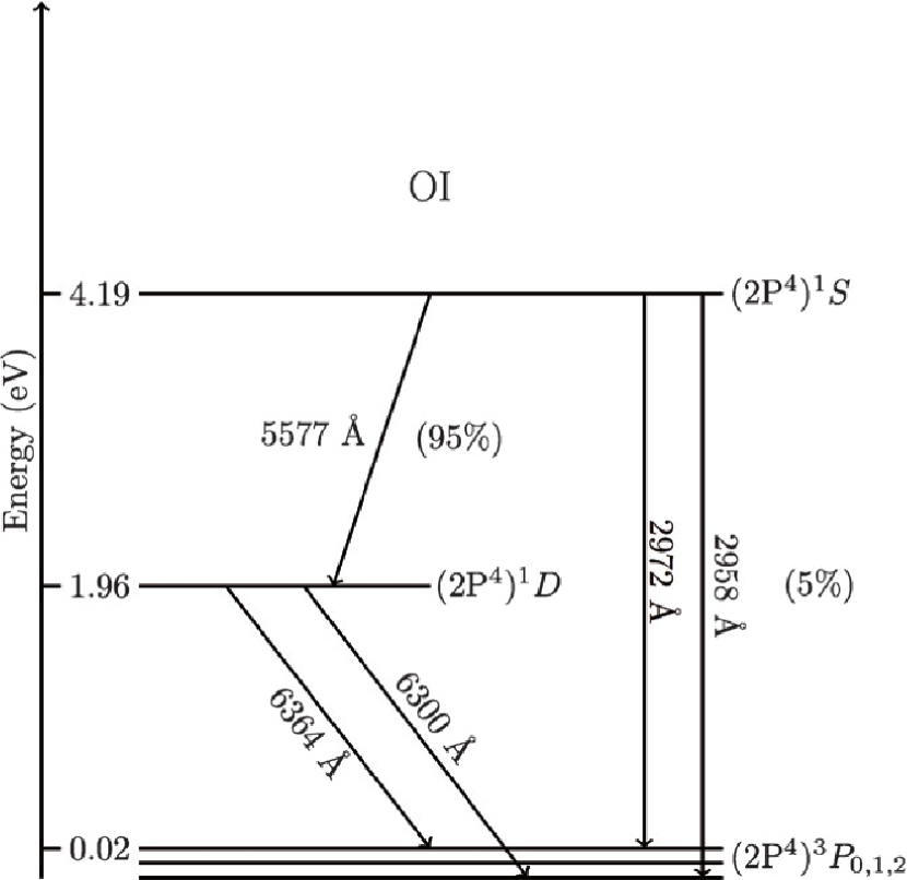
Figure 1:

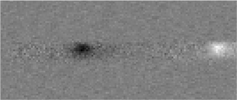
Figure 2:

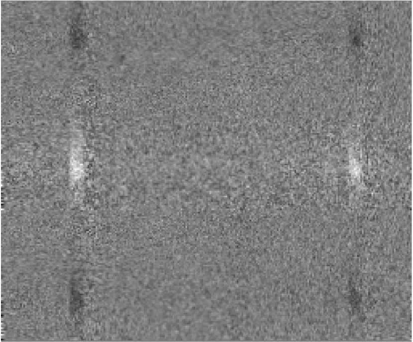
Figure 3:

Figure 4:

Figure 5:

Figure 6:

Figure 7:

Figure 8:

Figure 9:

Figure 10:

References

- A’Hearn et al. (2011) M. F. A’Hearn, M. J. S. Belton, W. A. Delamere, L. M. Feaga, D. Hampton, J. Kissel, K. P. Klaasen, L. A. McFadden, K. J. Meech, H. J. Melosh, P. H. Schultz, J. M. Sunshine, P. C. Thomas, J. Veverka, D. D. Wellnitz, D. K. Yeomans, S. Besse, D. Bodewits, T. J. Bowling, B. T. Carcich, S. M. Collins, T. L. Farnham, O. Groussin, B. Hermalyn, M. S. Kelley, M. S. Kelley, J.-Y. Li, D. J. Lindler, C. M. Lisse, S. A. McLaughlin, F. Merlin, S. Protopapa, J. E. Richardson, and J. L. Williams. EPOXI at Comet Hartley 2. Science, 332:1396–, June 2011. doi: 10.1126/science.1204054.
- A’Hearn et al. (2012) M. F. A’Hearn, L. M. Feaga, H. U. Keller, H. Kawakita, D. L. Hampton, J. Kissel, K. P. Klaasen, L. A. McFadden, K. J. Meech, P. H. Schultz, J. M. Sunshine, P. C. Thomas, J. Veverka, D. K. Yeomans, S. Besse, D. Bodewits, T. L. Farnham, O. Groussin, M. S. Kelley, C. M. Lisse, F. Merlin, S. Protopapa, and D. D. Wellnitz. Cometary Volatiles and the Origin of Comets. Astrophysical Journal, 758:29, October 2012. doi: 10.1088/0004-637X/758/1/29.
- Belton and Melosh (2009) M. J. S. Belton and J. Melosh. Fluidization and multiphase transport of particulate cometary material as an explanation of the smooth terrains and repetitive outbursts on 9P/Tempel 1. Icarus, 200:280–291, March 2009. doi: 10.1016/j.icarus.2008.11.012.
- Bhardwaj and Raghuram (2012) A. Bhardwaj and S. Raghuram. A Coupled Chemistry-emission Model for Atomic Oxygen Green and Red-doublet Emissions in the Comet C/1996 B2 Hyakutake. Astrophysical Journal, 748:13, March 2012. doi: 10.1088/0004-637X/748/1/13.
- Bockelée-Morvan et al. (2012) D. Bockelée-Morvan, N. Biver, B. Swinyard, M. de Val-Borro, J. Crovisier, P. Hartogh, D. C. Lis, R. Moreno, S. Szutowicz, E. Lellouch, M. Emprechtinger, G. A. Blake, R. Courtin, C. Jarchow, M. Kidger, M. Küppers, M. Rengel, G. R. Davis, T. Fulton, D. Naylor, S. Sidher, and H. Walker. Herschel measurements of the D/H and 16O/18O ratios in water in the Oort-cloud comet C/2009 P1 (Garradd). Astronomy and Astrophysics, 544:L15, August 2012. doi: 10.1051/0004-6361/201219744.
- Bodewits et al. (2014) D. Bodewits, T. L. Farnham, M. F. A’Hearn, L. M. Feaga, A. McKay, D. G. Schleicher, and J. M. Sunshine. The Evolving Activity of the Dynamically Young Comet C/2009 P1 (Garradd). Astrophysical Journal, 786:48, May 2014. doi: 10.1088/0004-637X/786/1/48.
- Capria et al. (2002) M.T. Capria, G. Cremonese, A. Bhardwaj, and M.C. de Sanctis. O1S and O1D emission lines in the spectrum of 153P/2002 C1 (Ikeya-Zhang). Astronomy and Astrophysics, 442(3):1121–1126, 2002.
- Capria et al. (2008) M.T. Capria, G. Cremonese, A. Bhardwaj, M.C. de Sanctis, and E.E. Mazzotta. Oxygen emission lines in the high resolution spectra of 9P/Tempel 1 following the deep impact event. Astronomy and Astrophysics, 479(1):257–263, 2008.
- Clough et al. (2005) SA Clough, MW Shephard, EJ Mlawer, JS Delamere, MJ Iacono, K Cady-Pereira, S Boukabara, and PD Brown. Atmospheric radiative transfer modeling: A summary of the aer codes. Journal of Quantitative Spectroscopy and Radiative Transfer, 91(2):233–244, 2005.
- Cochran (2008) A.L. Cochran. Atomic oxygen in the comae of comets. Icarus, 198(1):181–188, 2008.
- Cochran and Cochran (2001) A.L. Cochran and W.D. Cochran. Observations of O (1S) and O (1D) in spectra of C/1999 S4 (LINEAR). Icarus, 154(2):381–390, 2001.
- Combes et al. (1988) M. Combes, J. Crovisier, T. Encrenaz, V. I. Moroz, and J.-P. Bibring. The 2.5-12 micron spectrum of Comet Halley from the IKS-VEGA Experiment. Icarus, 76:404–436, December 1988. doi: 10.1016/0019-1035(88)90013-9.
- Combi et al. (2004) M. Combi, W. Harris, and W. Smyth. Gas dynamics and kinetics in the cometary coma: Theory and observations. In Comets II, pages 523–552, Tucson, AZ, USA, 2004. University of Arizona Press.
- Combi et al. (2013) M. R. Combi, J. T. T. Mäkinen, J.-L. Bertaux, E. Quémerais, S. Ferron, and N. Fougere. Water production rate of Comet C/2009 P1 (Garradd) throughout the 2011-2012 apparition: Evidence for an icy grain halo. Icarus, 225:740–748, July 2013. doi: 10.1016/j.icarus.2013.04.030.
- Crovisier (1989) J. Crovisier. The photodissociation of water in cometary atmospheres. Astronomy and Astrophysics, 213(1–2):459–464, 1989.
- Crovisier (1997) J. Crovisier. Infrared observations of volatile molecules in comet Hale-Bopp. Earth, Moon, and Planets, 79(1/3):125–143, 1997.
- Decock et al. (2013) A. Decock, E. Jehin, D. Hutsemékers, and J. Manfroid. Forbidden oxygen lines in comets at various heliocentric distances. Astronomy and Astrophysics, 555:A34, July 2013. doi: 10.1051/0004-6361/201220414.
- Dello Russo et al. (1998) N. Dello Russo, M. A. Disanti, M. J. Mumma, K. Magee-Sauer, and T. W. Rettig. Carbonyl Sulfide in Comets C/1996 B2 (Hyakutake) and C/1995 O1 (Hale-Bopp): Evidence for an Extended Source in Hale-Bopp. Icarus, 135:377–388, October 1998. doi: 10.1006/icar.1998.5990.
- Delsemme (1980) A. H. Delsemme. Photodissociation of CO2 into CO plus O/1D/. In I. Dubois and G. Herzberg, editors, Les Spectres des Molécules Simples au Laboratoire et en Astrophysique, pages 515–523, 1980.
- DiSanti et al. (2003) M. A. DiSanti, M. J. Mumma, N. Dello Russo, K. Magee-Sauer, and D. M. Griep. Evidence for a dominant native source of carbon monoxide in Comet C/1996 B2 (Hyakutake). Journal of Geophysical Research (Planets), 108:5061, June 2003. doi: 10.1029/2002JE001961.
- DiSanti et al. (2014) M. A. DiSanti, G. L. Villanueva, L. Paganini, B. P. Bonev, J. V. Keane, K. J. Meech, and M. J. Mumma. Pre- and post-perihelion observations of C/2009 P1 (Garradd): Evidence for an oxygen-rich heritage? Icarus, 228:167–180, January 2014. doi: 10.1016/j.icarus.2013.09.001.
- Farnham et al. (2013) T. Farnham, D. Bodewits, L. M. Feaga, M. F. A’Hearn, J. M. Sunshine, D. D. Wellnitz, K. P. Klaasen, and T. W. Himes. Imaging Comets ISON and Garradd With the Deep Impact Flyby Spacecraft. In AAS/Division for Planetary Sciences Meeting Abstracts, volume 45 of AAS/Division for Planetary Sciences Meeting Abstracts, page 407.08, October 2013.
- Feaga et al. (2014) L. M. Feaga, M. F. A’Hearn, T. L. Farnham, D. Bodewits, J. M. Sunshine, A. M. Gersch, S. Protopapa, B. Yang, M. Drahus, and D. G. Schleicher. Uncorrelated Volatile Behavior during the 2011 Apparition of Comet C/2009 P1 Garradd. Astronomical Journal, 147:24, January 2014. doi: 10.1088/0004-6256/147/1/24.
- Feaga et al. (2007) L.M. Feaga, M.F. A’Hearn, J.M. Sunshine, O. Groussin, and T.L. Farnham. Asymmetries in the distribution of H2O and CO2 in the inner coma of comet 9P/Tempel 1 as observed by Deep Impact. Icarus, 190(2):345–356, 2007.
- Festou (1981) M.C. Festou. The density distribution of neutral compounds in cometary atmospheres I - models and equations. Astronomy and Astrophysics, 95(1):69–79, 1981.
- Festou and Feldman (1981) M.C. Festou and P.D. Feldman. The forbidden oxygen lines in comets. Astronomy and Astrophysics, 103(1):154–159, 1981.
- Gersch and A’Hearn (2014) A. M. Gersch and M. F. A’Hearn. Coupled Escape Probability for an Asymmetric Spherical Case: Modeling Optically Thick Comets. Astrophysical Journal, 787:36, May 2014. doi: 10.1088/0004-637X/787/1/36.
- Haser (1957) L. Haser. Distribution d’intensite dans la tete d’une comete. Bull. Acad. R. Sci. Liege, 43:740–750, 1957.
- Hogg et al. (2001) D. W. Hogg, D. P. Finkbeiner, D. J. Schlegel, and J. E. Gunn. A Photometricity and Extinction Monitor at the Apache Point Observatory. Astronomical Journal, 122:2129–2138, October 2001. doi: 10.1086/323103.
- Huebner et al. (1992) W.F. Huebner, J.J. Keady, and S.P. Lyon. Solar photo rates for planetary atmospheres and atmospheric pollutants. Astrophysics and Space Science, 195(1):1–289, 291–294, 1992.
- Huestis et al. (2008) D. L. Huestis, S. W. Bougher, J. L. Fox, M. Galand, R. E. Johnson, J. I. Moses, and J. C. Pickering. Cross Sections and Reaction Rates for Comparative Planetary Aeronomy. Space Science Reviews, 139:63–105, August 2008. doi: 10.1007/s11214-008-9383-7.
- Magee-Sauer et al. (1990) K. Magee-Sauer, F. Scherb, F. L. Roesler, and J. Harlander. Comet Halley O(1D) and H2O production rates. Icarus, 84:154–165, March 1990. doi: 10.1016/0019-1035(90)90163-4.
- McKay et al. (2012) A. J. McKay, N. J. Chanover, J. P. Morgenthaler, A. L. Cochran, W. M. Harris, and N. D. Russo. Forbidden oxygen lines in Comets C/2006 W3 Christensen and C/2007 Q3 Siding Spring at large heliocentric distance: Implications for the sublimation of volatile ices. 220:277–285, July 2012. doi: 10.1016/j.icarus.2012.04.030.
- McKay et al. (2013) A. J. McKay, N. J. Chanover, J. P. Morgenthaler, A. L. Cochran, W. M. Harris, and N. D. Russo. Observations of the forbidden oxygen lines in DIXI target Comet 103P/Hartley. Icarus, 222:684–690, February 2013. doi: 10.1016/j.icarus.2012.06.020.
- McKay et al. (2014) A. J. McKay, N. J. Chanover, M. A. DiSanti, J. P. Morgenthaler, A. L. Cochran, W. M. Harris, and N. D. Russo. Rotational variation of daughter species production rates in Comet 103P/Hartley: Implications for the progeny of daughter species and the degree of chemical heterogeneity. Icarus, 231:193–205, March 2014. doi: 10.1016/j.icarus.2013.11.029.
- Meech and Svoren (2004) K. Meech and J. Svoren. Physical and chemical evolution of cometary nuclei. In Comets II, pages 317–335, Tucson, AZ, USA, 2004. University of Arizona Press.
- Morgenthaler et al. (2001) J.P. Morgenthaler, W.M. Harris, F. Scherb, C. Anderson, R.J. Oliversen, N.E. Doane, M.R. Combi, M.L. Marconi, and W.H. Smyth. Large aperture [O I] 6300 photometry of comet Hale-Bopp: Implications for the photochemistry of OH. Astrophysical Journal, 563(1):451–461, 2001.
- Morgenthaler et al. (2007) J.P. Morgenthaler, W.M. Harris, and M.R. Combi. Large Aperture O I 6300 Å Observations of Comet Hyakutake: Implications for the Photochemistry of OH and O I Production in Comet Hale-Bopp. Astrophysical Journal, 657:1162–1171, March 2007. doi: 10.1086/511062.
- Ootsubo et al. (2012) T. Ootsubo, H. Kawakita, S. Hamada, H. Kobayashi, M. Yamaguchi, F. Usui, T. Nakagawa, M. Ueno, M. Ishiguro, T. Sekiguchi, J.-i. Watanabe, I. Sakon, T. Shimonishi, and T. Onaka. AKARI Near-infrared Spectroscopic Survey for CO2 in 18 Comets. Astrophysical Journal, 752:15, June 2012. doi: 10.1088/0004-637X/752/1/15.
- Paganini et al. (2012) L. Paganini, M. J. Mumma, G. L. Villanueva, M. A. DiSanti, B. P. Bonev, M. Lippi, and H. Boehnhardt. The Chemical Composition of CO-rich Comet C/2009 P1 (Garradd) AT R h = 2.4 and 2.0 AU before Perihelion. Astrophysical Journal Letters, 748:L13, March 2012. doi: 10.1088/2041-8205/748/1/L13.
- Pittichová et al. (2008) J. Pittichová, C. E. Woodward, M. S. Kelley, and W. T. Reach. Ground-Based Optical and Spitzer Infrared Imaging Observations of Comet 21P/GIACOBINI-ZINNER. Astronomical Journal, 136:1127–1136, September 2008. doi: 10.1088/0004-6256/136/3/1127.
- Raghuram and Bhardwaj (2014) S. Raghuram and A. Bhardwaj. Photochemistry of atomic oxygen green and red-doublet emissions in comets at larger heliocentric distances. Astronomy and Astrophysics, 566:A134, June 2014. doi: 10.1051/0004-6361/201321921.
- Reach et al. (2009) W. T. Reach, J. Vaubaillon, M. S. Kelley, C. M. Lisse, and M. V. Sykes. Distribution and properties of fragments and debris from the split Comet 73P/Schwassmann-Wachmann 3 as revealed by Spitzer Space Telescope. Icarus, 203:571–588, October 2009. doi: 10.1016/j.icarus.2009.05.027.
- Reach et al. (2013) W. T. Reach, M. S. Kelley, and J. Vaubaillon. Survey of cometary CO2, CO, and particulate emissions using the Spitzer Space Telescope. Icarus, 226:777–797, September 2013. doi: 10.1016/j.icarus.2013.06.011.
- Schultz et al. (1992) D. Schultz, G. S. H. Li, F. Scherb, and F. L. Roesler. Comet Austin (1989c1) O(1D) and H2O production rates. Icarus, 96:190–197, April 1992. doi: 10.1016/0019-1035(92)90072-F.
- Sharpee and Slanger (2006) BD Sharpee and TG Slanger. O (1d2-3p2, 1, 0) 630.0, 636.4, and 639.2 nm forbidden emission line intensity ratios measured in the terrestrial nightglow. The Journal of Physical Chemistry A, 110(21):6707–6710, 2006.
- Slanger et al. (2011) Tom G Slanger, Brian D Sharpee, Dušan A Pejaković, David L Huestis, Manuel A Bautista, Richard L Gattinger, Edward J Llewellyn, Ian C McDade, David E Siskind, and Kenneth R Minschwaner. Atomic oxygen emission intensity ratio: Observation and theory. Eos, Transactions American Geophysical Union, 92(35):291, 2011.
- Spinrad (1982) H. Spinrad. Observations of the red auroral oxygen lines in nine comets. Publications of the Astronomical Society of the Pacific, 94:1008–1016, December 1982. doi: 10.1086/131101.
- Szabó et al. (2012) G. M. Szabó, L. L. Kiss, A. Pál, C. Kiss, K. Sárneczky, A. Juhász, and M. R. Hogerheijde. Evidence for Fresh Frost Layer on the Bare Nucleus of Comet Hale-Bopp at 32 AU Distance. Astrophysical Journal, 761:8, December 2012. doi: 10.1088/0004-637X/761/1/8.
- Tseng et al. (2007) W.-L. Tseng, D. Bockelée-Morvan, J. Crovisier, P. Colom, and W.-H. Ip. Cometary water expansion velocity from OH line shapes. Astronomy and Astrophysics, 467:729–735, May 2007. doi: 10.1051/0004-6361:20066666.
- Villanueva et al. (2011) G. L. Villanueva, M. J. Mumma, M. A. Disanti, B. P. Bonev, E. L. Gibb, K. Magee-Sauer, G. A. Blake, and C. Salyk. The molecular composition of Comet C/2007 W1 (Boattini): Evidence of a peculiar outgassing and a rich chemistry. Icarus, 216:227–240, November 2011. doi: 10.1016/j.icarus.2011.08.024.
- Villanueva et al. (2012a) G. L. Villanueva, M. J. Mumma, B. P. Bonev, R. E. Novak, R. J. Barber, and M. A. Disanti. Water in planetary and cometary atmospheres: H2O/HDO transmittance and fluorescence models. Journal of Quantitative Spectroscopy and Radiative Transfer, 113:202–220, February 2012a. doi: 10.1016/j.jqsrt.2011.11.001.
- Villanueva et al. (2012b) G. L. Villanueva, M. J. Mumma, M. A. DiSanti, B. P. Bonev, L. Paganini, and G. A. Blake. A multi-instrument study of Comet C/2009 P1 (Garradd) at 2.1 AU (pre-perihelion) from the Sun. Icarus, 220:291–295, July 2012b. doi: 10.1016/j.icarus.2012.03.027.
- Wang et al. (2003) S.-i. Wang, R. H. Hildebrand, L. M. Hobbs, S. J. Heimsath, G. Kelderhouse, R. F. Loewenstein, S. Lucero, C. M. Rockosi, D. Sandford, J. L. Sundwall, J. A. Thorburn, and D. G. York. ARCES: an echelle spectrograph for the Astrophysical Research Consortium (ARC) 3.5m telescope. In M. Iye and A. F. M. Moorwood, editors, Instrument Design and Performance for Optical/Infrared Ground-based Telescopes, volume 4841 of Society of Photo-Optical Instrumentation Engineers (SPIE) Conference Series, pages 1145–1156, March 2003. doi: 10.1117/12.461447.
- Wu and Chen (1993) C.Y.R. Wu and F.Z. Chen. Velocity distibutions of hydrogen atoms and hydroxyl radicals produced through solar photodissociation of water. Journal of Geophysical Research, 98(E4):7415–7435, 1993.
- Yamamoto (1981) T. Yamamoto. Molecular distribution in the comae of H2O-comets - an analytic model. Moon and Planets, 24:175–188, April 1981. doi: 10.1007/BF00910607.
- Yang and Drahus (2012) B. Yang and M. Drahus. Submillimeter Spectroscopic Observations of C/2009 P1 with the JCMT Telescope. LPI Contributions, 1667:6322, May 2012.