Spectral properties and control of an exciton trapped in a multi-layered quantum dot

Abstract

The spectral properties of one exciton trapped in a self-assembled multi-layered quantum dot is obtained using a high precision variational numerical method. The exciton Hamiltonian includes the effect of the polarization charges, induced by the presence of the exciton in the quantum dot, at the material interfaces. The method allows to implement rather easily the matching conditions at the interfaces of the hetero-structure. The numerical method also provides accurate approximate eigenfunctions that enable the study of the separability of the exciton eigenfunction in electron and hole states. The separability, or the entanglement content, of the total wave function allows a better understanding of the spectral properties of the exciton and, in particular, shed some light about when the perturbation theory calculation of the spectrum is fairly correct or not. Finally, using the approximate spectrum and eigenfunctions, the controlled time evolution of the exciton wave function is analyzed when an external driving field is applied to the system. It is found that it is possible to obtain pico and sub-picoseconds controlled oscillations between two particular states of the exciton with a rather low leakage of probability to other exciton states, and with a simple pulse shape.

I Introduction

The calculation of the spectral properties of an exciton trapped in a semiconductor nano-structure is a long standing problem. Even in the case of the most simple model used to study this system, i.e. the one band effective mass approximation (EMA), there is a number of subtle details that it is necessary to take into account. In particular, when the nano-structure consists in a heterogeneous quantum dot, the mismatch between the different material parameters imposes boundary conditions to the particle wave functions and the electrostatic potential between the electron and hole that form the exciton can not be taken as the simple Coulomb potential Delerue2004 ; Ferreyra(1998) .

The presence of excitons can be easily spotted in the absorption spectrum of different semiconductors. The energy associated to each absorption peak is smaller to the energy difference between the electronic energy levels that lie on the semiconductor valence band and those that lie on the semiconductor conduction band. If the electrons in the semiconductor were independent between them and no many-body effects were present, the absorption energy should be equal to the energy difference between two electronic levels, one located in the conduction band and the other located in the valence band. But, when an electron is promoted from the lower band to the upper one, by radiation absorption for instance, the “hole” produced interacts with the electron, and the binding of the pair gives place to the exciton. The energy difference observed in the absorption spectrum, with respect to the values that correspond to independent electrons, is precisely given by the binding energy between the pair electron-hole Cardona(2005) ; Bastard(1988) .

An exciton trapped in a quantum dot or in a given nano-structure has very different physical properties compared to a bulk one. Roughly speaking, the radius associated to the exciton is, more or less, of the same magnitude order than the characteristic length of many nano-structures. This can be used to tune the physical trait of interest using the material parameters of the semiconductors employed in the nano-structure, its geometry and its size to tailor different properties. For instance, the mean life time of the exciton can be adjusted depending on the application in mind. Recently, some Quantum Information Processing (QIP) proposals use an exciton trapped in a quantum dot as qubit, in which case the basis states are given by the presence ($\left|1\right\rangle$), or absence ($\left|0\right\rangle$), of the exciton Troiani(2000) ; Biolatti(2000) . Obviously, for QIP applications the life time of the exciton should be larger than the time needed to operate and control the qubit.

Modeling an exciton in a particular physical situation can be a tricky business, since a plethora of effective Hamiltonians are available to use. Starting from the multi-band many-electrons Hamiltonian, there is a number of ways to derive effective Hamiltonians which usually decompose the one-electron wave function in an “envelop part” and a “Bloch part”. The Bloch part accounts for the underlying periodical lattice structure of the semiconductor and the envelop part for the specific nano-structure under consideration. If the electron is not confined, i.e. belongs to the bulk of the material, the envelop part is reduced to the usual imaginary exponential present in the wave functions allowed by the Bloch theorem. Otherwise, when a nano-structure is present, the effective Hamiltonians for the envelop part resemble a multicomponent Schrödinger-like equations. Probably, the most well know procedure to derive effective-Hamiltonians is the k.p method Voon(2009) . The number of components of the Hamiltonian derived using the k.p method depends on how much information about the semiconductor band structure is incorporated. For instance, the well-known eight-band model is derived using the fact that the valence band levels have orbital angular momentum quantum number $L=1$, the conduction band levels $L=0$, and the electronic spin has $s=1/2$ Haug(2004) .

In this work we consider the simplest two-band effective mass approximation model (EMA) for an exciton, trapped in a spherical Type -I device, with a core, well, and barrier structure. The core and the barrier semiconductor compound is exactly the same, while the well semiconductor is characterized by a conduction band whose bottom energy is lower than the corresponding energy of the material that form the core and the external barrier. The gap between the conduction band and the valence band is narrower for the well semiconductor, than the gap for the core one. Consequently, the confinement potential for the electron and the hole are given by the profiles of the conduction and valence bands of the semiconductors that form the device. This model has been studied extensively because, despite its apparent simplicity, allows to obtain accurately the spectrum of different QD accurately in a wide variety of situations. Anyway, there are some features on it that ask for some careful treatment. The first feature that must be handled with care is owed to the model binding potential, since this is assumed as given by the profile of the semiconductor bands, a step-like potential results for both, the electron and the hole. Moreover, since the effective mass of both, the electron and the hole, are assumed as discontinuous position dependent functions, the Hermitian character of the kinetic energy is assured only with appropriate matching conditions for the wave functions at the interfaces between different materials. Finally, the electrostatic potential between the electron and hole can not be taken as the simple Coulomb potential. It has been shown that polarization terms should be included because, again, of the presence of interfaces between materials with different dielectric constants Ferreyra(1998) .

It is worth to mention that the study of the properties of excitons confined in quantum dots Woggon(1995) has been tackled using a number of methods, like perturbation theory Chang(1998) ; Schooss(1994) , the k.p method Pokatilov(2001) ; Efros(1998) , and with different types of confinement potential as the infinite potential well Ferreyra(1998) or the parabolic one Garm(1996) . The selection of potentials and method are often dictated by the application in mind, that could range from excitonic lasers Bimberg(1997) ; Bimberg(2005) , through quantum information processing Kamada(2004) ; Chen(2001) ; Biolatti(2002) , up to one-electron transistors Ishibashi(2003) in micro electronics devices. Between the physical phenomena that have received more attention, it can be mentioned the binding energy Lelong(1996) , the decoherence Calarco(2003) ; Bonadeo(1998)A ; Bonadeo(1998)B and the Stark effect Billaud(2009) among many others.

To study the two-band EMA model described above we calculated its spectrum and eigen-states using a variational approach. The approach allows us to take into account the matching conditions at the interfaces of the device and the (quite) complicated interaction potential between the two parts of the exciton that includes the effects of polarization. As we shall see, our approach allows us to obtain highly accurate approximate results for the spectrum and approximate wave functions that provide information about the entanglement content of the two-particle quantum state. This information gives useful information about the parameter range where the two-particle wave function can be more or less accurately taken as the product of one-particle wave functions. The manuscript is organized as follows: in Section II the variational method to obtain the spectrum of one or two-particle Hamiltonians is discussed and presented in some detail, In Section III the electron-hole pair EMA Hamiltonian is analyzed paying some attention to the electrostatic problem originated by the geometry and composition of the quantum dot and the binding energy of the electron-hole pair is calculated, in Section IV the separability problem of the exciton wave function is presented and analyzed, in particular it is shown that the characterization through a measure of separability gives a better understanding of the exciton spectral properties. The time evolution of the exciton wave function when an external driving field is applied to the QD is studied in Section V. The study is intended to look for regimes where the external driving allows to switch between only two pre-selected states of the exciton, with a negligible or controllable leakage of probability to other exciton states. Finally, our results are discussed and summarized in Section VI

II One body models and methods

The EMA approximation, when applied to the description of an independent electron (e), or hole (h), is characterized by a number of parameters such as the effective mass of the particle or the energy band gap of the materials from which is made the quantum dot. Otherwise, the Hamiltonian associated to it seems like an ordinary Schrödinger-like Hamiltonian

$$\mathcal{H}_{e(h)}=-\frac{\hbar^{2}}{2}\nabla_{e(h)}\left(\frac{1}{m_{e(h)}^{*}(r_{e(h)})}\nabla_{e(h)}\right)+V_{e(h)}(r_{e(h)})+V_{s}(r_{e(h)})$$ (1)

where $m_{e(h)}^{*}(r_{e(h)})$ is the electron (hole) effective mass. For an one-band model, $m_{e}^{*}$ corresponds to the the effective mass of the electron in the conduction band, while $m_{h}^{*}$ is taken as the light effective mass of the hole in the valence band. $V_{e(h)}(r_{e(h)})$ is the binding potential for the electron (hole).

Figure 1a) shows a cartoon of the spherical self assembled quantum dot under consideration. The inner core, of radius $a$, and the outer shell (also called clad) are made of the same compound, let us call it two (2), while the middle layer, of radius $b$, is made of a different compound, let us call it one (1). These kind of hetero structures are termed of Type I or II, if the top energy of the valence band of the middle layer material, $E^{1}_{top}$, is larger than the top energy of the valence band of material two, $E^{2}_{top}$, i.e. the hetero structure is of Type I if $E^{1}_{top}>E^{2}_{top}$, otherwise is of Type II, as can be seen clearly in Figure 1 b). The cartoon in Figure 1b) shows the conduction and valence bands profile as a function of the radial distance from the center of the hetero-structure.

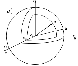
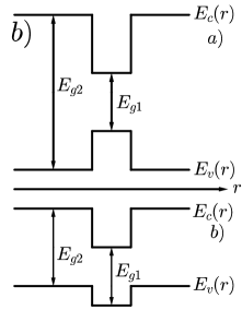
Figure 1: a) The cartoon shows the structure of the spherical self-assembled quantum dot. The different layers correspond to, from the center and going in the radial direction, the core whose radius $a$ and dielectric constant are shown, the potential well, with inner radius $a$ and exterior radius $b$, and the clad. b) The profiles of the conduction band, $E_{c}(r)$, and of the valence band, $E_{v}(r)$, for both a Type-I device (top) and a a Type-II devive (bottom). $E_{g}1$ and $E_{g}2$ are the gap energies of the potential well material and the core/clad material, respectively.

Since the potential in Equation 1, $V_{e(h)}(r_{e(h)})$, is taken as exactly the conduction band profile (valence band profile) for the electron (hole), it is clear that a Type-I device corresponds to the case where the middle layer acts as a potential well for both particles, so

$$V_{e(h)}(r)=\left\{\begin{array}[]{lcl}V_{0}^{e(h)}>0&&0<r<a\\ 0&&a<r<b\\ V_{0}^{e(h)}>0&&b<r\end{array}\right.,$$ (2)

and $V_{0}^{e(h)}=const.$

The potential $V_{s}$ is owed to the polarization charges produced at the interfaces core/middle layer and middle layer/clad because of the mismatch between their dielectric constants. It can be shown that the auto-polarization potential is given by

$$V_{s}(r)=\frac{q^{2}}{2\,\varepsilon_{1}}\sum_{l}\frac{1}{(1-pq)}\left(qr^{2l}+\frac{p}{r^{2l+1}}+\frac{pq}{r}\right)$$ (3)

where

$$p=(\varepsilon_{1}-\varepsilon_{2})la^{(2l+1)}/[\varepsilon_{2}l+\varepsilon_{1}(l+1)],$$ (4)

and

$$q=(\varepsilon_{1}-\varepsilon_{2})(l+1)b^{-(2l+1)}/[\varepsilon_{1}l+\varepsilon_{2}(l+1)].$$ (5)

The kinetic energy term in Equation 1 is written in a symmetric fashion in order to guarantee the Hermitian character of the operator, if it is considered together with the following matching conditions

$$\psi(r=a^{-}) = \psi(r=a^{+})$$ (6)

$$\psi(r=b^{-}) = \psi(r=b^{+})$$

$$\left(\frac{1}{m^{*}}\frac{d\psi}{dr}\right)|_{r=a^{-}} = \left(\frac{1}{m^{*}}\frac{d\psi}{dr}\right)|_{r=a^{+}}$$

$$\left(\frac{1}{m^{*}}\frac{d\psi}{dr}\right)|_{r=b^{-}} = \left(\frac{1}{m^{*}}\frac{d\psi}{dr}\right)|_{r=b^{+}}.$$

The eigenvalue problem

$$\mathcal{H}\psi=E\psi,$$ (7)

with $\mathcal{H}$ given by Equation 1 can be studied using different (an numerous) methods that result in an approximate spectrum and, in some cases, approximate eigenfunctions. Anyway, the matching conditions can not be implemented in a direct way depending on which method is used to tackle the problem. A method that allows to weight adequately the matching conditions is one that incorporates easily the step-like nature of the binding potential, Equation 2, and the effective mass. The approximate eigenfunctions and eigenvalues analyzed in this work were obtained using B-splines basis sets, which have been used to obtain high accuracy results for atomic, molecular and quantum dot systems. The method has been well described elsewhere, so the only details that we discus here are the relevant ones to understand some of results presented later on.

To use the B-splines basis, the normalized one-electron orbitals are given by

$$\phi_{n}({r})=C_{n}\,\frac{B^{(k)}_{n+1}(r)}{r}\,;\;\;n=1,\ldots$$ (8)

where $B^{(k)}_{n+1}(r)$ is a B-splines polynomial of order $k$. The numerical results are obtained by defining a cutoff radius $R$, and then the interval $[0,R]$ is divided into $I$ equal subintervals. B-spline polynomials deboor (for a review of applications of B-splines polynomials in atomic and molecular physics, see Reference bachau01 , for its application to QD problems see Reference Ferron2013 ) are piecewise polynomials defined by a sequence of knots $t_{1}=0\leq t_{2}\leq\cdots\leq t_{2k+I-1}=R$ and the recurrence relations

$$B_{i}^{(1)}(r)\,=\,\left\{\begin{array}[]{ll}1&\mbox{if}\,t_{i}\leq r<t_{i+1}\\ 0&\mbox{otherwise,}\end{array}\right.\,.$$ (9)

$$B_{i}^{(k)}(r)\,=\,\frac{r-t_{i}}{t_{i+k-1}-t_{i}}\,B_{i}^{(k-1)}(r)\,+\,\frac{t_{i+k}-r}{t_{i+k}-t_{i+1}}\,B_{i}^{(k-1)}(r)\;(k>1)\,.$$ (10)

The standard choice for the knots in atomic physics bachau01 is $t_{1}=\cdots=t_{k}=0$ and $t_{k+I}=\cdots=t_{2k+I-1}=R$. Because of the matching conditions at the interfaces between the core and the potential well and between the potential well and the clad, it is more appropriate to choose the knots as follows: at the extremes of the interval $\left[0,R\right]$ where the wave function is calculated, there are $k$ knots that are repeated, while at the interfaces $r=a$ and $r=b$ there are $k-3$ knots that are repeated, and in the open intervals $(0,a)$, $(a,b)$ and $(b,R)$ the knots are distributed uniformly HaoXue(2002)

The constant $C_{n}$ in Equation 8 is a normalization constant obtained from the condition $\left\langle\phi_{n}|\phi_{n}\right\rangle=1$

$$C_{n}=\frac{1}{\left[\int_{0}^{R}\,\left(B^{(k)}_{n+1}(r)\right)^{2}\,dr\right]^{1/2}}\,.$$ (11)

Because $B_{1}(0)\neq 0$ and $B_{I+3k-9}(R)\neq 0$, we have $N=I+3k-11$ orbitals corresponding to $B_{2},\ldots,B_{I+3k-10}$. In all the calculations we used the value $k=5$, and, we do not write the index $k$ in the eigenvalues and coefficients.

Figure 2: The first one-electron eigenvalues for a infinite potential well (dashed lines) and for a finite potential well (solid lines) as functions of the dimensionless ratio $a/b$. In both cases, $b=31.71$ nm, that is the Bohr radius for an exciton immersed in a HgS matrix. The eigenvalues correspond to zero angular momentum ($\ell=0$) states.

To gain some insight about the performance of the B-spline method we first studied the eigenvalue problem of one electron confined in a multi-layered quantum dot as the one depicted in Figure 1a). The quantum dots whose core, well and clad are made of CdS/HgS/CdS have been extensively studied Schooss(1994) , so it is a good starting point to our study. For these materials, the effective masses for the electron in their respective conduction bands are $m_{e,CdS}^{*}=0.2$, $m_{e,HgS}^{*}=0.036$, while for the hole in the valence bands the effective masses are given by $m_{h,CdS}^{*}=0.7$, $m_{h,HgS}^{*}=0.040$. The dielectric constants are $\varepsilon_{CdS}=\varepsilon_{2}=5.5$, $\varepsilon_{HgS}=\varepsilon_{1}=11.36$. Besides,

$$E^{CdS}_{bottom}-E^{HgS}_{bottom} = 1.35\mbox{eV},$$

$$E^{HgS}_{top}-E^{CdS}_{top} = 0.9\mbox{eV}.$$

The other parameters that define the device are the radii $a$ and $b$. To augment the effect of the confinement owed to the binding potential we choose $b$ equal to the Bohr radius of a bulk exciton in HgS Chang(1998) , then $a$ can take any value between zero and $b$. This model was studied in Ferreyra(1998) considering the limit of “strong confinement”, i.e. the electron is bound in an infinite potential well. We want to remark that the electro-hole pair behaves very much as a hydrogen-like atom when it is immersed in a semiconductor bulk besides, in many cases, the hole effective mass is much larger than electron one. So, it makes sense to consider the Bohr radius as one of the length scales that characterize the problem.

Figure 2 shows the behavior of the lowest lying approximate one-electron eigenvalues obtained using the B-spline method for a quantum dot with the material parameters listed above, and for one electron bound in an infinite potential well, as functions of the ratio between both radii, $a/b$. The eigenvalues corresponds to eigenfunctions with orbital angular momentum with quantum number $\ell=0$. As can be observed from the Figure, the infinite potential well eigenvalues, that can be obtained exactly, are a pretty good approximation to the quantum dot eigenvalues for small values of $a/b$, but for larger values of $a/b$, or for the excited states, the relative error grows considerably. Since in many works in the literature, the binding energy of the exciton is obtained using the exact solutions of the infinite potential well, the results shown in Figure 2 indicate that it is necessary to proceed with great caution if this approximation were to be used. The eigenvalues obtained using the B-spline method have a relative error of less than $10^{-3}$.

Figure 3: The lowest lying one-electro eigenvalues for different radial ($n_{r}$) and angular momentum ($\ell$) quantum numbers. The eigenvalues were calculated for a finite potential well and the Hamiltonian includes the auto-polarization term in Equation 3 (solid lines). The dashed lines are the corresponding eigenvalues obtained taking out the autopolarization term (or equivalently choosing $\varepsilon_{1}=\varepsilon_{2}$). The labels for each curve are the quantum numbers that identify the corresponding eigenstate.

There has been some discussion about the need to include, or not, the self polarization term, Equation 3, in the one electron Hamiltonian, Equation 1 Delerue2004 . Figure 3 shows the behaviour of the lowest lying energy eigenvalues, for several orbital angular momentum quantum numbers, and with, or without, the auto-polarization term. Is is clear that for $a/b<0.4$, and for all the angular momentum quantum numbers shown, that the auto-polarization term changes the eigenvalues in a, approximately, 10$\%$ , showing that for large quantum dot the auto-polarization contribution can not be ignored. When $a$ grows up to $b$ the effect becomes less and less important. Other way to characterize the phenomenology is the following, if the eigenvalues become independent of $\ell$ for a given radial quantum number $n$, i.e. the energy eigenvalues depends almost only on $n$, then the well potential becomes “small enough” and the auto-polarization term becomes negligible. In this limit, the polarization term and the angular momentum part of the kinetic energy can be treated as perturbations.

It is interesting to point that despite that the hole Hamiltonian is determined by different parameters than the electron one, the behavior of its spectrum is very similar, for that reason we do not include a detailed analysis of it. On the other hand, once the electron and hole approximate eigenfunctions are obtained, a plot of them reveals that both particles are well localized inside the potential well. Besides, the repetition of knots at the interfaces enables that the approximate solutions meet the matching conditions, Equation 6, to a high degree of accuracy.

III Two-particle model

The Hamiltonian for an exciton formed by an electron and a hole can be written as

$$\mathcal{H}_{ex}=\mathcal{H}_{e}+\mathcal{H}_{h}+V_{c}({\mathbf{r}}_{e},{\mathbf{r}}_{h}),$$ (12)

where $\mathcal{H}_{e}$ and $\mathcal{H}_{h}$ are the one-body Hamiltonians of Equation 1, and $V_{c}({\mathbf{r}}_{e},{\mathbf{r}}_{h})$ is the electrostatic potential between the electron and hole. Usually, one is tempted to consider $V_{c}$ as the usual Coulomb potential between a positive charge and a negative one but, if the exciton is confined to an hetero-structure made of different materials, this approach oversimplifies the situation.

Having in mind the argument of the paragraph above, we consider a better a approximation for the actual electrostatic potential that was suggested by Ferreyra and Proetto Ferreyra(1998) . Since the hole is usually “heavier” than the electron, and that the scenario of most interest occurs when both particle are well localized, it is simpler to consider $V_{c}$ as the solution to the Poisson equation considering that the hole and electron coordinates are restricted to the potential well, i.e.

$$V_{c}({\mathbf{r}}_{e},{\mathbf{r}}_{h})=q_{e}q_{h}\,G({\mathbf{r}}_{e},{\mathbf{r}}_{h}),$$ (13)

where

$$\nabla_{r}^{2}G({\mathbf{r}},{\mathbf{r}}^{\prime})=\left\{\begin{array}[]{lcl}-\frac{4\pi}{\varepsilon_{1}}\delta({\mathbf{r}}-{\mathbf{r}}^{\prime})&&\mbox{if}\;a<r<b\\ 0&&\mbox{otherwise}\end{array}\right.,$$ (14)

Figure 4: The binding energy expectation value as a function of the ratio $a/b$. The curves are grouped in two bundles, the higher one was calculated including all the polarization effects originated by the dielectric constants mismatch, $\varepsilon_{1}\neq\varepsilon_{2}$ , while the lower one ignores the mismatch and takes $\varepsilon_{1}=\varepsilon_{2}$. In each bundle, the curve at the top (solid line) corresponds to the exciton ground state. As the binding energy is a decreasing function of the exciton eigen-energy, in each bundle the lower and lower lying curves correspond to the first excited state, to the second one, ans so successively. The sudden drop of the curves observed for large enough values of the ratio $a/b$ show where each level reach the “ionization threshold”.

So, solving Equation 14, it can be shown that the electrostatic potential that gives the interaction between the electron and the hole can be written as

$$V_{c}(\mathbf{r}_{e},\mathbf{r}_{h}) = q_{e}q_{h}\sum_{l,m}Y_{lm}^{*}(\theta_{h},\varphi_{h})Y_{lm}(\theta_{e},\varphi_{e})$$ (16)

$$\quad\times\frac{4\pi}{\varepsilon_{1}(2l+1)(1-pq)}$$

$$\quad\times[r_{<}^{l}+pr_{<}^{l+1}][r_{>}^{-(l+1)}+qr_{>}^{l}],$$

where

$$p=(\varepsilon_{1}-\varepsilon_{2})la^{(2l+1)}/[\varepsilon_{2}l+\varepsilon_{1}(l+1)],$$ (17)

$$q=(\varepsilon_{1}-\varepsilon_{2})(l+1)b^{-(2l+1)}/[\varepsilon_{1}l+\varepsilon_{2}(l+1)],$$ (18)

and

$$r_{>(<)}=max(min)\{r_{e},r_{h}\}.$$ (19)

The exciton binding energy can be obtained as the expectation value of the electrostatic potential

$$E_{binding}^{\alpha}=-\langle\psi_{\alpha}|V_{c}(\mathbf{r}_{e},\mathbf{r}_{h})|\psi_{\alpha}\rangle,$$ (20)

where $|\psi_{\alpha}\rangle$ is an eigenstate of the exciton Hamiltonian, Equation 12.

Figure 4 shows the behavior of the binding energy as a function of the radii ratio $a/b$. For clarity, we restrict the curves shown to those data obtained with eigenfunctions with orbital angular momentum quantum numbers $l_{e}=l_{h}=m_{e}=m_{h}=0$. The Figure shows two well defined separated sets of curves. The lower set of curves correspond to the binding energy calculated without polarization terms (or equivalently putting $\varepsilon_{1}=\varepsilon_{2}$ in Equations 16,17 and 18). The upper set of curves corresponds to the binding energy calculated considering all the polarization effects ($\varepsilon_{1}\neq\varepsilon_{2}$). The polarization terms, owed to the polarization charges at the interfaces between the different materials, does not change the qualitative behavior of the binding energy but, at least for the parameters of Figure 4, not including them leads to an underestimation of the binding energy of approximately 100% . The inclusion of the polarization terms in the electrostatic potential increases the binding energy since for $\varepsilon_{1}>\varepsilon_{2}$ the correction terms in Equation 16, with respect to the Coulomb potential, have all the same sign.

IV separability of the exciton eigenfunctions

The availability of accurate numerical approximations for the actual exciton eigenfunctions gives the possibility to analyze their separability, in particular in this Section we analyze the behavior of the von Neumann entropy associated to the excitonic quantum state. We will show that some features of the binding energy already described in the precedent Section, can be understood best studying simultaneously both quantities. In particular, the analysis of the separability of the quantum states can shed some light about when the interaction between the exciton components can be treated using perturbation theory. Besides, there are some quantities that determine the strength of the interaction of the exciton with external fields, as the dipole moment, or expectation values that can not be accurately obtained if the correlation between the electron and hole is not taken into account.

A well known separability measure of the quantum state is the von Neumann entropy, $S$, which can be calculated as

$$S=-\sum_{k}\lambda_{k}\;\ln(\lambda_{k}),$$ (21)

where $\lambda_{k}$ are the eigenvalues of the electron reduced density matrix $\rho^{red}(\mathbf{r}_{e},\mathbf{r}^{\prime}_{e})$ which, if the quantum state of the exciton is given by a vector state $\psi(\mathbf{r}_{e},\mathbf{r}_{h})$, then

$$\rho^{red}(\mathbf{r}_{e},\mathbf{r}_{e}^{\prime})=\int\psi^{\star}(\mathbf{r}_{e},\mathbf{r}_{h})\psi(\mathbf{r}_{e}^{\prime},\mathbf{r}_{h})\;d\mathbf{r}_{h}.$$ (22)

Figure 5: a) The von Neummann entropy for the first few eigenstates, the lowest curve corresponds to the ground state eigenstate (label 0), the following to the second excited eigenstate (label 2) and so on. The inset shows a detailed view of the fundamental state von Neumann entropy. b) The binding energy for the ground state calculated following different methods. From top to bottom the curves were obtained with the full Hamiltonian and the B-spline method (solid line), without the auto-polarization terms (i.e. neglecting $V_{s}(r)$) and the B-spline method (dot-dashed line), again with the full Hamiltonian but using perturbation theory (dashed line) and finally without the auto-polarization terms and using perturbation theory (double-dot dashed line), respectively. For details see the text

Figure 5a shows the behavior of the von Neumann entropy as a function of the ratio $a/b$, for the approximate eigenfunctions of the first low lying exciton eigenvalues calculated using the B-spline method. As can be appreciated from the figure, the von Neumann entropy is a monotone decreasing function of the ratio $a/b$, i.e. the electron and hole became more and more independent (separable its wave function) when the radius of the core is increased. This is expected, but even for the ground state the effect of the non-separability of the excitonic wave function has a rather large influence in the binding energy, as can been appreciated in panel b). The von Neumann entropy, on the other hand is larger for the exciton excited states so, at least in principle, any effect related to the non-separability of the exciton wave function should be stronger for the excited states.

Figure 5b shows the behaviour of the groud state binding energy, again as a function of the ratio $a/b$, obtained using different methods. The top curve corresponds to the binding energy calculated with the B-spline approximation while, in decreasing order, the figure also shows the curves that correspond to the binding energy calculated with the B-spline method but without including the auto-polarization terms, besides the binding energy calculated using perturbation theory with and without the auto-polarization terms. The binding energy curve obtained using perturbation theory shows the first order approximation energy calculated using the finite potential well electron and hole eigenfunctions as the unperturbed levels.

At least for this set of parameters and materials, taking into account the auto-polarization terms has less influence than using a method (the B-splines) that takes into account the non-separability of the two-particle wave function. For the ground state the worst case scenario, perturbation theory without auto-polarization, differs from the best one, B-splines plus auto-polarization terms, by about five percent. Of course, since the self-assembled quantum dots offer a huge amount of different combinations of materials, geometries and sizes the quantitative results may change more or less broadly.

Figure 6 shows the binding energy obtained with the same methods that were used to obtain the data in Figure 5b), as describe above, but for an exciton in a different quantum dot. In this case, we considered a quantum dot formed by core/well/barrier structure made of ZnS/CdSe/ZnS. All the necessary parameters to determine the Hamiltonian, effective masses, dielectric constants, etc, can be found in Reference Schooss(1994) .

Figure 6: The ground state exciton binding energy vs $a/b$ for a device with core,well and clad made of ZnS/CdSe/ZnS. The curves are obtained following the same prescription than those shown in Figure 5. All the materials parameters can be found in Reference Chang(1998) . It is easy to appreciate that for this device the influence of the auto-polarization terms is smaller that in the first device analyzed, but the difference between the values obtained using perturbation theory and the B-spline method is larger

For the case shown in Figure 6, the influence of the auto-polarization terms is even smaller that in the first case analyzed, Figure 5, and the difference between the best and worst scenarios defined above is around seven, eight percent.

V control

There are two important applications of excitons in which the speed with which you can go from having to not having a exciton is crucial: the controlled and rapid photon production and the switching between the basis states of the qubit logically associated to the exciton. The physical process is exactly the same, but the motivation and requirements depend on which application is being considered. In this section we are interested in estimating how much we can force an excitonic qubit so that it oscillates periodically between its basis states with the highest possible frequency and a small probability loss to other exciton eigenstates. The need to estimate how fast the qubit can be switched between its basis states comes from the limits imposed by the decoherence sources that are unavoidable and restrict seriously the total operation time in which the qubit would keep its quantum coherence. Moreover, we intend to achieve the switching between the basis states with the simplest control pulse, that is, a sinusoidal one. So, many times it is found reasonable to ask that, if $T_{S}$ is the switching time and $\tau$ the time scale associated to the decoherence processes present in the physical system, then $T_{S}\sim 10^{-4}\tau$.

The main source of decoherence in charge qubits is owed to the interaction of the charge carrier, the electron(s) trapped in the quantum dot, and the thermal phonon bath present in the semiconductor matrix. This is the reason why, in many cases, spin qubits are preferred although its control is more complicated and have more longer operation time. Since in the exciton case the strength of the coupling with the phonon bath depends on the difference between the electronic and hole wave functions, it is to be expected that the decoherence rate for qubits based on one exciton would be smaller than for a charge qubit based on one (or more) electrons trapped in a quantum dot. Ideally, when the potential wells for the electron and the hole have exactly the same depth, for equal effective masses, and in the limit of zero interaction, the coupling with the phonon bath almost disappears. In this sense, the separability of the electron-hole wave function provides a good measure to select the parameter region where the coupling of the exciton with the phonon bath is smaller. Consequently, since even for very low temperatures the decoherence produced by the phonon bath imposes a total operation time on the order of a few tens of nanoseconds for qubits based on multi-layered self-assembled quantum dots, then to be considered a putative useful qubit the switching time $T_{S}$ should be on the order of the picoseconds or sub-picoseconds.

The leaking of probability to other exciton eigenstates when an external driving is applied can be analyzed using the following unitary one-exciton Hamiltonian, which describes the interaction of the electron-hole dipolar moment, $\vec{d}$, with an external periodic field $\vec{E}(t)$ applied to the quantum dot Haug(2004)

$$\mathcal{H}_{int}(t)=-\vec{d}\ldotp\vec{E}(t),$$ (23)

which in second quantization formalism can be written as Haug(2004) ; Biolatti(2002)

$$\mathcal{H}_{int}(t)=-E(t)\sum_{nm}\left[\mu_{nm}^{*}a_{n}^{\dagger}b_{m}^{\dagger}+h.c\right],$$ (24)

where $a^{\dagger}_{n}$ is the creation operator of an electron in the conduction band, $b^{\dagger}_{m}$ is the creation operator of a hole in the valence band, $n$ and $m$ stand for the corresponding one-particle levels, and $\mu^{\star}_{nm}$ is the matrix element of the dipolar moment operator, given by

$$\mu_{nm}=\mu_{bulk}\int\phi_{n}^{e}(\vec{r})\phi_{m}^{h}(\vec{r})d^{3}r,$$ (25)

where $\mu_{bulk}$ is the dipolar moment corresponding to an electronic transition from the valence band to the conduction bandHaug(2004) ; Biolatti(2002) .

All the one- and two-particles quantities needed to determine the parameters in Equation 24 and the time evolution of the exciton state can be obtained using the B-spline method described in the preceding Sections. Moreover, since the B-spline method provides a very good approximation to all the exciton bound states the time evolution of the approximate exciton quantum state can be written as a sum over bound states as follows

$$\Psi(t)=\sum_{i}U_{i}(t)\psi_{i},$$ (26)

where the sum runs over the approximate bound states provided by the B-spline method, $\psi_{i}$, and the time-dependent coefficients $U_{(}t)$ can be calculated integrating a set of complex coupled ordinary differential equations. The number of ordinary differential equations is determined by how many bound states the B-spline method is able to find. In the cases analyzed from now on we considered up to thirty bound states. The numerical integration of the ordinary differential equation was performed using standard Runge-Kutta algorithms.

Before analyzing the behavior of the exciton time-evolution it is worth to remark that the model allows only one exciton but the electron-hole pair can occupy many different exciton eigenstates and not only those associated to the qubit. Also, the model does not allow the “ionization” of the quantum dot nor the spontaneous recombination of the electron-hole pair in the time scale associated to the periodic external driving.

As $|U_{0}|^{2}$ and $|U_{1}|^{2}$ are the probability that the exciton is in state $|0\rangle$ or in state $|1\rangle$ respectively, we use the leakage, $L$, to characterize the probability loss that experiments the qubit when the driving $E(t)=E_{0}\sin(\omega t)$ is applied. The leakage is defined as

$$L=\lim_{n\rightarrow\infty}\frac{1}{nT}\int_{t^{\prime}}^{t^{\prime}+nT}\;\left(1-|U_{0}|^{2}-|U_{1}|^{2}\right)\,dt\;,$$ (27)

where $T=2\pi/\omega$.

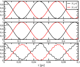
Figure 7: (color on-line) The time evolution of the occupation probabilities $|U_{0}|^{2}$ (black solid line) and $|U_{1}|^{2}$ (red solid line). The exciton is initialized, in all cases, in the fundamental state, so $|U_{0}(t=0)|^{2}=1$, and $|U_{i}(t=0)|^{2}=0$, $\forall i\neq 0$. From top to bottom, panel a) shows the time evolution for $E_{0}=1\times 10^{-3}$ eV/nm, panel b) for $E_{0}=1\times 10^{-2}$eV/nm and panel c) for $E_{0}=5\times 10^{-2}$eV/nm, respectively.

Form now on, we consider a CdS/HgS/CdS structure with $a=b/2$. Figure 7 shows the behavior of the occupation probabilities $|U_{0}|^{2}$ and $|U_{1}|^{2}$ as a function of time, for different external field strengths $E_{0}$. In the three cases shown, the frequency of the external driving is set equal to the resonance frequency $\omega_{res}$ of the exciton ground state. The resonance frequency, $\omega_{res}=(E_{0}+E_{g1})/\hbar$, where $E_{0}$ is the lowest eigenvalue calculated from the exciton Hamiltonian and $E_{g1}$ is the energy gap of material one, i.e. $E_{g1}=E^{gap}_{HgS}$.

From the different panels in Figure 7, it is possible to appreciate that switching times on the order of picoseconds or less are achievable for driving strengths small with no noticeable leakage. This scenario is further supported by the data shown in Figure 8.

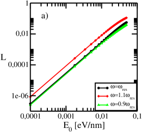
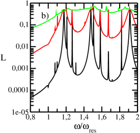
Figure 8: (color on-line) a) The leakage of probability vs the strength of the driving field. The linear dependency of $L$ with $E_{0}$, when the axis scale is log-log, can be clearly appreciated. From top to bottom, the Figure shows curves obtained for $\omega=0.9\omega_{res}$ (green line and symbols), $\omega=\omega_{res}$ (black line and symbols) and $\omega=1.1\omega_{res}$. The leakage for $\omega=0.9\omega_{res}$ is smaller than for $\omega=\omega_{res}$ because the qubit does not leaves the fundamental state. b) The leakage as a function of the external driving frequency for three different values of $E_{0}$. Here we use the same external driving strengths that in Figure 7. From bottom to top, $E_{0}=1\times 10^{-3}$ eV/nm (black line), $E_{0}=1\times 10^{-2}$eV/nm (red line) and $E_{0}=5\times 10^{-2}$eV/nm (green line).

Figure 8a) shows the leakage as a function of the strength of the external driving $E_{0}$ for several driving frequencies $\omega$. The data is shown in a $\log-\log$ scale, and under this assumption the leakage shows a linear behavior for a span of a few magnitude orders. The different curves correspond to different values of the driving frequency, but to analyze the dependency of the leakage with the driving frequency we choose to plot it at fixed values of the driving strength. Figure 8 shoes the behavior of the leakage as a function of the external drving frequency and for the three external driving strengths used in Figure 7. The different curves show a rich structure, and several spikes which are present in all the curves for the same frequencies. These spikes are owed to the presence of many one-exciton levels that are very close to the ground state energy. It is clear that to obtain low levels of leakage, besides an excellent tuning of the driving frequency, it is necessary to have well resolved exciton energy levels or, in other words, the nano-structure should be designed in such way that the exciton is formed in the non-perturbative regime, ı.e when the binding energy is as large as possible. This seems to advice the use of large potential wells, but there is a trade off to consider since the separation between the one-particle levels diminishes when the characteristic sizes of the potential well are increased. A simple way to enhance the interaction between electron-hole pair, at least in principle, is to choose materials whose combination provides a deep potential well and a low potential-well dielectric constant.

VI Conclusions and Discussion

One of the advantages of using the B-spline method is its adaptability to tackle problems with step-like parameters and matching conditions at the interface between different spatial regions. Similarly, the method allows to tackle complicated one or two-particle potentials, with a limited number of adaptations. The interaction potential between the electron and the hole, Equation 16 can be treated modifying the method usually employed with the Coulomb potential deboor , since both can be written as expansions in spherical harmonics.

As the analysis of the von Neumann entropy shows, for large QD (or small cores in our case) the perturbation theory calculations give a rather poor approximation for the binding energy. We can be fairly sure that our results, since they are variational, that predict smaller ground state energy for the exciton Hamiltonian, Equation 12, than other methods are more accurate than previous results. This implies that our results predict larger values for the exciton binding energy.

To avoid an excessive leakage of probability, it is mandatory to design a quantum dot such that the two lower states of the exciton are well separated from the other one-exciton states. Choosing materials that allow for a larger interaction between the electron and the hole seems to be an apparent solution.

- (1) C. Delerue and M. Lannoo, Nanostructures. Theory and Modelling (Springer, Berlin, 2004)
- (2) J. M. Ferreyra, and C. R. Proetto, Phys. Rev. B, 57, 9061 (1998).
- (3) M. Cardona, and Y. Y. Peter Fundamentals of semiconductors (Springer-Verlag, Berlin Heidelberg, 2005)
- (4) Bastard, G. (1988). Wave mechanics applied to semiconductors. Les editions de Physique (CNRS, Paris, 1988).
- (5) F. Troiani, U. Hohenester, and E. Molinari Phys. Rev. B 62, R2263(R) (2000).
- (6) E. Biolatti, R. C. Iotti, P. Zanardi, and F. Rossi, Phys. Rev. Lett. 85, 5647 (2000).
- (7) L.C. L. Y. Voon and M. Willatzen, The kp method: electronic properties of semiconductors. (Springer-Verlag, Berlin Heidelberg, 2009)
- (8) H. Haug, H., and S. W. Koch, Quantum theory of the optical and electronic properties of semiconductors. Fourth Edition (World Scientific Publishing Co. Pte. Ltd., Singapore, 2004)
- (9) U. Woggon and S. V. Gaponenko, Physica Status Solidi (b) 189, 285-343 (1995).
- (10) K. Chang and J. B. Xia, Phys. Rev. B 57, 9780 (1998)
- (11) D. Schooss, A. Mews, A. Eychmüller, and H. Weller, Phys. Rev. B, 49, 17072 (1994).
- (12) E. P. Pokatilov, V. A. Fonoberov, V. M. Fomin, and J. T. Devreese, Phys. Rev. B 64, 245329 (2001).
- (13) A. L. Efros and M. Rosen, Phys. Rev. B 58, 7120 (1998).
- (14) T. Garm, T, J. Phys.: Condens. Matter 8, 5725 (1996).
- (15) Bimberg, D., Kirstaedter, N., Ledentsov, N. N., Alferov, Z. I., Kop’ev, P. S., and Ustinov, V. M. (1997). IEEE Journal of, 3(2), 196-205.
- (16) D. Bimberg, Journal of Physics D: Applied Physics 38, 2055 (2005).
- (17) H. Kamada and H. Gotoh, Semiconductor science and technology, 19, S392 (2004).
- (18) P. Chen, C. Piermarocchi, and L. J. Sham, Phys. Rev. Lett, 87, 067401 (2001).
- (19) E. Biolatti, I. D’Amico, P. Zanardi, and F. Rossi, Phys. Rev. B, 65, 075306 (2002).
- (20) K. Ishibashi, M. Suzuki, D. Tsuya, and Y. Aoyagi, Microelectronic engineering 67, 749-754 (2003).
- (21) T. Calarco,A. Datta, P. Fedichev, E. Pazy, and P. Zoller, Phys. Rev. A 68, 012310 (2003).
- (22) N. H. Bonadeo, G. Chen, D. Gammon, D. S. Katzer, D. Park, and D. G. Steel, Phys. Rev. Lett. 81, 2759 (1998).
- (23) N. H. Bonadeo, J. Erland, D. Gammon, D. Park, D. S. Katzer, and D. G. Steel, Science 282, 1473-1476 (1998).
- (24) P. Lelong and G. Bastard, Solid state communications 98, 819-823 (1996).
- (25) B. Billaud, M. Picco, and T. T. Truong, J. Phys.: Condens. Matter 21, 395302 (2009).
- (26) C. de Boor, A Practical Guide to Splines (Springer, New York, 2001)
- (27) H. Bachau, E. Cormier, P. Decleva, J. E. Hansen, and F. Martin, Rep. Prog. Phys. 64, 1815 (2001).
- (28) A. Ferrón, P. Serra and O. Osenda, J, Appl. Phys. 113, 134304 (2013)
- (29) HaoXue, Q. I. A. O., TingYun, S. H. I., and Baiwen, L. I. Commun. Theor. Phys. 37,221 (2002)