Evaluating the geometric measure of multiparticle entanglement

Abstract

We present an analytical approach to evaluate the geometric measure of multiparticle entanglement for mixed quantum states. Our method allows the computation of this measure for a family of multiparticle states with a certain symmetry and delivers lower bounds on the measure for general states. It works for an arbitrary number of particles, for arbitrary classes of multiparticle entanglement, and can also be used to determine other entanglement measures.

I Introduction

The characterization of quantum correlations is central for many applications such as quantum metrology or quantum simulation. Moreover, the quantification of quantum correlations allows to study quantum phase transitions and is also relevant for quantum optics experiments, where coherent dynamics of many particles should be certified. This characterization, however, is difficult as for multiparticle systems different forms of entanglement exist. To give a simple example, a quantum state $|\psi\rangle$ on three particles can be fully separable, $|\psi_{fs}\rangle=|a\rangle\otimes|b\rangle\otimes|c\rangle$, or entangled on two particles, but separable for the third one. An instance of such a biseparable state is $|\psi_{bs}\rangle=|\phi_{ab}\rangle\otimes|\eta_{c}\rangle$, which is biseparable with respect to the $AB|C$-partition, but there are two other possible bipartitions. Finally, if a state is not fully separable or biseparable, it is called genuine multiparticle entangled. For more than three particles even more classes are possible. Here, a pure state is called $k$-separable, if the $N$ particles can be split into $k$ unentangled groups. The case $k=N$ corresponds to the fully separable states, while $k=2$ denotes the biseparable states gtreview .

So far, this is only a classification for pure states. In order to study multiparticle entanglement in realistic situations, two extensions are necessary: First, one needs to deal with mixed states, as they occur naturally in experiments. Second, one needs to quantify entanglement in order to go beyond the simple entangled vs. separable scheme measure-reviews . A popular way to quantify multiparticle entanglement makes use of the geometric measure of entanglement wei . For that, one defines for pure states via

$$E_{G}^{(k)}(|\psi\rangle)=1-\max_{|\phi\rangle{\rm\;is\\ \;\;k-sep.}}|\langle\phi|\psi\rangle|^{2}$$ (1)

the amount of entanglement as one minus the maximal overlap over pure $k$-separable states. Clearly, this vanishes for $k$-separable pure states and the measure is large for highly entangled states where the overlap is small. Note that the quantity $E_{G}^{(k)}$ distinguishes between the different classes of $k$-separability, so it is indeed a whole family of entanglement measures suited for all the different entanglement classes illuminati . The geometric measure found many applications, it can be used to characterize the distinguishability of quantum states by local means geo-apps and to investigate quantum phase transitions in spin models geo-spin , to mention only a few. Moreover, it is directly linked to other entanglement measures, which quantify the distance to the separable states streltsov .

The quantity needs to be extended to mixed quantum states. For that, one uses the so-called convex roof construction. One defines

$$E_{G}^{(k)}(\varrho)=\min_{p_{i},|\psi_{i}\rangle}\sum_{i}p_{i}E_{G}^{(k)}(|\psi_{i}\rangle),$$ (2)

where the minimization is taken over all possible decompositions $\varrho=\sum_{i}p_{i}|{\psi_{i}}\rangle\!\langle{\psi_{i}}|$ into pure states. This is a typical method to extend a pure state entanglement measure to the mixed state case, but obviously this minimization is difficult to perform. So far, only in some special cases the evaluation of the geometric measure for mixed states is possible wei ; gbb ; indiaposter . Analytical results on the evaluation of the convex roof for other measures have to date mainly be obtained for the bipartite measure of the concurrence and measures with a related mathematical structure wootters . Further results are typically restricted to special families of states or special entanglement classes eltschka ; furtherexact or require a numerical optimization geza-neu .

In this paper, we present an analytical way to evaluate the geometric measure of entanglement for mixed states of $N$ qubits. Our approach gives the exact value for a class of states, for other states the approach results in a lower bound on the measure. The method works for an arbitrary number of qubits and arbitrary kinds of $k$-separability. Since it has been shown that computing the geometric measure is equivalent to determining other distance related entanglement measures streltsov , our results constitute one of the most detailed characterizations of multiparticle entanglement so far.

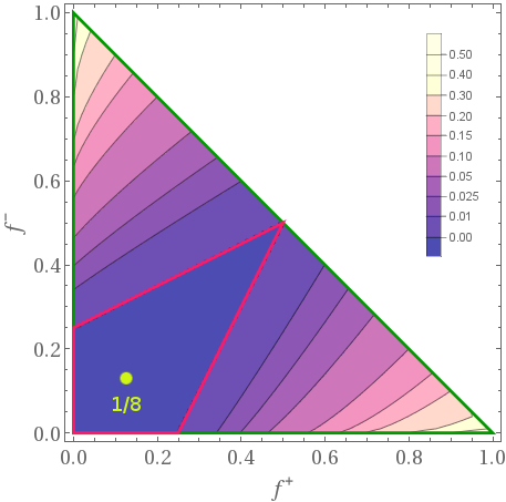
Figure 1: The triangle of the GHZ-symmetric states for three qubits. The states are parameterized by the two fidelities $f^{+}$ and $f^{-}$ and include besides the GHZ states also the maximally mixed state $\openone/8$. The values of the geometric measure of entanglement $E_{G}^{(3)}$ are shown as contours, and the red deltoid denotes the parameter region where the states are fully separable, so the geometric measure vanishes.

II GHZ-symmetric states

We start by defining a two-parameter family of states that we use for our study. Consider three qubits and the states

$$\varrho^{\rm ghz} (f^{+},f^{-})=f^{+}|GHZ^{+}\rangle\!\langle GHZ^{+}|$$

$$+f^{-}|GHZ^{-}\rangle\!\langle GHZ^{-}|+(1-f^{+}-f^{-})\frac{\Pi}{6},$$ (3)

where $|GHZ^{\pm}\rangle=(|000\rangle\pm|111\rangle)/\sqrt{2}$ are two Greenberger-Horne-Zeilinger (GHZ) states, $\Pi=\openone-|GHZ^{+}\rangle\!\langle GHZ^{+}|-|GHZ^{-}\rangle\!\langle GHZ^{-}|$ is the projector onto the space orthogonal to the GHZ states, and $f^{\pm}\in[0,1]$ with $f^{+}+f^{-}\leq 1$. This family of states forms a triangle in the state space (see also Fig. 1) and includes besides the GHZ states also the maximally mixed state $\openone/8=\varrho^{\rm ghz}(1/8,1/8).$ We note that states of this form have been studied before and recently, Eltschka and Siewert succeeded by computing the three-tangle as an entanglement measure for them eltschka . In the following, we will call this family of states GHZ-symmetric states.

Before discussing our main results, we note some symmetries of the states. We have

$$\varrho^{\rm ghz}=U\varrho^{\rm ghz}U^{\dagger},$$ (4)

where either (i) $U$ induces a permutation of the qubits or (ii) $U=\sigma_{x}\otimes\sigma_{x}\otimes\sigma_{x}$ is a spin-flip operation on all three qubits or (iii) $U$ describes correlated qubit rotations of the form $U(\alpha,\beta,\gamma)=e^{i\alpha\sigma_{z}}\otimes e^{i\beta\sigma_{z}}\otimes e^{i\gamma\sigma_{z}}$ with $\alpha+\beta+\gamma=0.$ In fact, one can easily see that the states $\varrho^{\rm ghz}$ are the only states invariant under these operations eltschka .

From this it follows that the states $\varrho^{\rm ghz}$ have, for any convex entanglement measure obeying the additional constraint of being permutation-invariant horosym , the minimal entanglement among all states with the same GHZ fidelities $f^{+}$ and $f^{-}$. This can be seen as follows: The transformations (i), (ii) and (iii) from above do not change the amount of entanglement. So, if an arbitrary state $\varrho$ is symmetrized with respect to a given unitary, $\varrho\mapsto(\varrho+U\varrho U^{\dagger})/2$, the entanglement measure will not increase due to its convexity. After symmetrization with respect to all three transformations the state $\varrho$ is made GHZ-symmetric. The fidelities $f^{+}$ and $f^{-}$ are invariant under the symmetrization since the GHZ states $|GHZ^{\pm}\rangle$ are invariant, but the entanglement is decreasing, which proves the claim.

This minimality is not only convenient for computing the geometric measure, it is also useful for experiments: An experimenter who has not full information about the quantum state may only measure the fidelities $f^{+}$ and $f^{-}$ and compute the entanglement of the GHZ-symmetric states with our formulas below. The resulting value is automatically a lower bound on the different forms of multiparticle entanglement present in the experiment. If more information on the state is available, one may even optimize $f^{+}$ and $f^{-}$ under local transformations eltschka2 .

III Results for three qubits

We consider the geometric measure for full separability $E_{G}^{(3)}$, where the overlap with fully separable states is taken. The corresponding measure for genuine multiparticle entanglement will be considered later. We can directly state:

Observation 1. Let $\varrho^{\rm ghz}$ be a GHZ-symmetric state of three qubits. Then, the geometric measure is given by

$$E_{G}^{(3)}=\!\!\max_{\mu\in[0,1]}\frac{1}{2}\big{[}1+\mu(2f^{+}-1)-\sqrt{\alpha}+\frac{f^{-}\mu(\mu+\sqrt{\alpha})}{\mu-1}\big{]},$$ (5)

where we used the abbreviation $\alpha=1-\mu+\mu^{2}.$ This formula holds for $f^{+}\geq f^{-}$, for the other case one has to exchange the values of $f^{+}$ and $f^{-}$.

The idea of the proof is the following: The entanglement $E_{G}^{(3)}$ is the minimal entanglement compatible with the fidelities $f^{+}$ and $f^{-}$. As the measure is defined via the convex roof, the minimal entanglement is convex, too. This convex function can be expressed with the help of the Legendre transformation legendretrafo . So one has to compute the Legendre transform of the geometric measure, and from that one can compute the geometric measure itself. The detailed proof, however, involves some nontrivial optimizations and the use of criteria for full separability of quantum states and is given in the Appendix.

To start the discussion, one may wonder why the computation of the geometric measure still contains a remaining optimization. The main reason is notational simplicity: The remaining optimization can analytically be evaluated for any given $f^{+},f^{-}$ by setting the derivative with respect to $\mu$ equal zero. In fact, even a closed formula for arbitrary $f^{+},f^{-}$ is possible compi , the final result, however, is quite lengthy and does not lead to new insights. In Fig. 1 we show the value of the geometric measure according to Observation 1. Note that for $f^{+}\leq(2f^{-}+1)/4$ and $f^{-}\leq(2f^{+}+1)/4$ the state is PPT and hence fully separable. This was was known before duer01 ; kay , extensions of this statement will be discussed below.

For important subfamilies of GHZ-symmetric states, closed formulas can directly be written down. First, one may be interested in the hypotenuse of the triangle, where $f^{+}+f^{-}=1.$ For this case and $f^{+}\geq f^{-}$ our method gives

$$E_{G}^{(3)}=\frac{1}{2}(1-\sqrt{1-(2f^{+}-1)^{2}}),$$ (6)

in agreement with previous results gbb . Second, for the lower cathetus (where $f^{-}=0$) one finds that

$$E_{G}^{(3)} = \frac{1}{4}\big{[}1+2f^{+}-2\sqrt{3}\sqrt{f^{+}(1-f^{+})}\big{]}$$

$$\mbox{ for }f^{+}\in[1/4,3/4],$$

$$E_{G}^{(3)} = f^{+}-1/2\;\;\;\mbox{ for }f^{+}\in[3/4,1].$$ (7)

Given the values of $E_{G}^{(3)}$ it is interesting to ask about the structure and form of the optimal decomposition in the convex roof. This does not only demonstrate the complete understanding of the problem, it can also be used to determine the closest separable state with respect to the Uhlmann fidelity streltsov . We find that the optimal decomposition for the lower cathetus for $f^{+}\in[1/4,3/4]$ consists of 28 states. One of them is the state

$$|\psi_{1}\rangle =\alpha(|000\rangle+|111\rangle)$$

$$+\beta(|001\rangle+|010\rangle+|011\rangle+|100\rangle+|101\rangle+|110\rangle)$$ (8)

with $\alpha=\sqrt{f^{+}/2}$ and $\beta=\sqrt{(1-2\alpha^{2})/6}=\sqrt{(1-f^{+})/6}$ and the other vectors are obtained by applying transformations of the type $e^{i\phi_{1}\sigma_{z}}\otimes e^{i\phi_{2}\sigma_{z}}\otimes e^{i\phi_{3}\sigma_{z}}$ to $|\psi_{1}\rangle.$ For $f^{+}\in[3/4,1]$ the optimal decomposition is of the type $\varrho(f^{+})=(1-p)\varrho^{\rm ghz}(3/4,0)+p|GHZ^{+}\rangle\!\langle GHZ^{+}|$, explaining the linear behavior of $E_{G}^{(3)}$. The details are given in the Appendix.

IV The case of $N$ qubits and $k$-separability

We can easily extend the family of GHZ-symmetric states to an arbitrary number of qubits by replacing $|GHZ^{+}\rangle$ and $|GHZ^{-}\rangle$ with the corresponding $N$-qubit GHZ states and considering

$$\varrho^{\rm ghz} = f^{+}|GHZ^{+}_{N}\rangle\!\langle GHZ^{+}_{N}|+f^{-}|GHZ^{-}_{N}\rangle\!\langle GHZ^{-}_{N}|$$ (9)

$$+(1-f^{+}-f^{-})\frac{\Pi_{N}}{2^{N}-2}$$

where $\Pi_{N}$ is now a projector onto a the $2^{N}-2$-dimensional space orthogonal to the GHZ states. This family of states obeys analogous symmetries as the three-qubit states. The reader may notice at this point that the $N$-qubit GHZ-symmetric states are not uniquely determined by the symmetries. This means that it is not clear from the beginning that a lower bound based on the fidelities $f^{+}$ and $f^{-}$ gives the exact value of the entanglement. We will see later that this is nevertheless the case, for the moment we just state:

Observation 2. Let $\varrho^{\rm ghz}$ be an $N$-qubit GHZ-symmetric quantum state and $E_{G}^{(k)}$ the geometric measure with respect to $k$-separability with $3\leq k\leq N$. Then, this measure is given by:

$$E_{G}^{(k)}(f^{+},f^{-})$$ (10)

$$=\max_{\mu\in[0,\mu_{\rm max}]}\frac{1}{2}\big{[}1+\mu(2f^{+}-1)-\sqrt{\gamma}+\frac{f^{-}\mu(\mu+\sqrt{\alpha})}{\mu-1}\big{]},$$

where we have used $\mu_{\rm max}=2^{k-3}/(2^{k-2}-1)$ and $\gamma=(\mu-1)^{2}+2^{3-k}\mu$ and $\alpha=1-\mu+\mu^{2}.$ The proof is given in the Appendix.

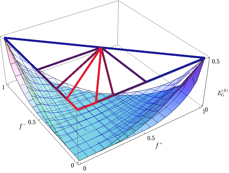
Figure 2: The geometric measure of entanglement for four qubits. From top to bottom, the different values for full separability ($k=4$), three-separability ($k=3$) and biseparability ($k=2$) are shown. The square and the deltoids on the top denote the regions, where the measures vanish.

Note that this formula does not depend on the number of qubits, but on the parameter $k$ characterizing the separability. Also, for the case $k=3$ we have $\gamma=\alpha$, and the expression reduces to Eq. (5). Finally, it remains to consider the case $k=2$, i.e. the geometric measure for genuine multiparticle entanglement. In this case, we obtain a very simple solution:

Observation 3. The geometric measure of genuine multiparticle entanglement is for arbitrary GHZ-symmetric states given by

$$E_{G}^{(2)}(f^{+},f^{-})=\frac{1}{2}-\sqrt{f(f-1)},$$ (11)

where $f=\max\{f^{+},f^{-}\}$ is the larger of the two fidelities. The formula is valid if $f\geq 1/2$, otherwise the state is biseparable. The proof is given in the Appendix.

Equipped with these results, we can visualize the geometric measure for the different classes, an example is provided in Fig. 2. We add that from our proof it follows that an arbitrary $k$-separable multi-qubit state has to fulfill the conditions

$$f^{+}\leq\frac{1}{2^{k-1}}\big{[}1+(2^{k-1}-2){f^{-}}\big{]},$$

$$f^{-}\leq\frac{1}{2^{k-1}}\big{[}1+(2^{k-1}-2){f^{+}}\big{]},$$ (12)

see also Eq. (41) in the Appendix. Applied to the GHZ-symmetric states, these equations describe deltoid curves where the states are $k$-separable and where the corresponding measures vanish. These are also shown in Fig. 2.

V Connections to other entanglement measures

An interesting feature of the geometric measure is the fact that it is intimately connected to other measures streltsov ; martin . This allows to determine other measures from our results on the geometric measure. More importantly, however, this connection enables us to prove properties of the geometric measure.

Let us first recall the central result of Ref. streltsov . The Uhlmann fidelity between two mixed states is given by

$$F(\varrho,\sigma)=[Tr(\sqrt{\sqrt{\varrho}\sigma\sqrt{\varrho}})]^{2}=[Tr(|\sqrt{\varrho}\sqrt{\sigma}|)]^{2}.$$ (13)

This can been used to define several types of distance-based entanglement measures, such as the Bures measure of entanglement $E_{B}(\varrho)=\min_{\sigma\in S}[2-2\sqrt{F(\varrho,\sigma)}],$ where $S$ denotes the set of separable states, or the Groverian measure of entanglement, $E_{GV}(\varrho)=\min_{\sigma\in S}\sqrt{1-F(\varrho,\sigma)}.$ In Ref. streltsov it was shown that the geometric measure for mixed states obeys

$$E_{G}(\varrho)=1-\max_{\sigma\in S}F(\varrho,\sigma).$$ (14)

This means that calculating the convex roof of the geometric measure is equivalent to finding the closest separable state, which is a remarkable connection between two seemingly different optimization problems. It also shows that our results on the geometric measure can directly be used to determine the distance based measures mentioned above.

In order to use this result for a better understanding of the geometric measure, we note some properties of the Uhlmann fidelity karol . First, it is unitarily invariant, $F(U\varrho U^{\dagger},U\sigma U^{\dagger})=F(\varrho,\sigma)$. Then, for a given $\varrho$ the quantity $F(\varrho,\sigma)$ is concave in $\sigma.$ Finally, it is monotonous under quantum operations, $F(\Lambda[\varrho],\Lambda[\sigma])\geq F(\varrho,\sigma)$ for any completely positive map $\Lambda$. From this property and Eq. (14) it follows that the geometric measure for a state $\varrho$ decreases under a positive map $\Lambda$, if the nearest separable state $\sigma$ is mapped onto a separable states, i.e. $E_{G}[\Lambda(\varrho)]\leq E_{G}(\varrho)$ if $\Lambda(\sigma)$ is separable. It also implies that the closest separable state to a GHZ-symmetric state is also GHZ-symmetric. Now we are able to show two results on the geometric measure:

First, we can see why the multi-qubit states in Eq. (9) minimize the geometric measure among all states with the fidelities $f^{+}$ and $f^{-}$, although they are not uniquely determined by the GHZ symmetry. Applying the GHZ symmetrization operations to an arbitrary quantum state can only decrease the value of $E_{G}$, so the state with the minimal $E_{G}$ and given fidelities will definitely be GHZ-symmetric. This means that the state looks already similar to the state in Eq. (9), but the diagonal elements $\varrho_{2,2},\dots,\varrho_{2^{N}-1,2^{N}-1}$ do not have to be identical. More precisely, for three qubits they have to be identical as in Eq. (3), but for four qubits there are two possibilities, depending on whether the number of excitations $|1\rangle\!\langle 1|$ in $\varrho_{ii}$ is even or odd. In any case, for this type of states the separability properties for fixed bipartitions are determined by the criterion of the positivity of the partial transpose duer01 and the separability deltoids as in Figs. 1,2 and Eq. (12), are still appropriate, see also the proof of Observation 2. We can consider a global permutation of the computational basis, which permutes $\varrho_{2,2},...,\varrho_{2^{N}-1,2^{N}-1}$ but leaves $\varrho_{1,1}$ and $\varrho_{2^{N},2^{N}}$ invariant. This is a unitary positive map, which for GHZ-symmetric states also maps separable states to separable states. It follows that the closest separable state is mapped to a separable state and so the geometric measure decreases, moreover, by applying a random permutation, the diagonal elements $\varrho_{2,2},...,\varrho_{2^{N}-1,2^{N}-1}$ will become all the same. This proves the claim.

Second, we can derive an alternative formulation of Observation 1, as one can compute the geometric measure by finding the nearest separable state. If we consider an entangled state with $f^{+}>f^{-}$ it follows that the closest separable state is at the border of the deltoid, where $f^{+}=1/4+f^{-}/2.$ Since the corresponding density matrices $\varrho$ and $\sigma$ are diagonal in the same basis, the Uhlmann fidelity can easily be evaluated and minimized over this line. This leads to:

Observation 4. For entangled GHZ-symmetric states of three qubits with $f^{+}>f^{-}$ the geometric measure is given by

$$E_{G}^{(3)}(\varrho)= 1-\max_{\mu\in[0,1/2]}\Big{[}\frac{1}{4}(\sqrt{3}\sqrt{1-f^{+}-f^{-}}\sqrt{1-2\mu}$$

$$+2\sqrt{f^{-}}\sqrt{\mu}+\sqrt{f^{+}}\sqrt{1+2\mu})^{2}\Big{]}.$$ (15)

Again, this formula can in principle be evaluated for any values of $f^{+},f^{-}$, but the solution then becomes technical. We stress, however, a crucial difference between Eq. (5) and Eq. (15): Eq. (5) holds for all values $f^{+}>f^{-}$, consequently the value vanishes for separable states. Eq. (15) holds for states which are known to be entangled, but it is non-vanishing and not correct for separable states. A more practical difference is that Eq. (5) seems to be better suited for obtaining closed expressions as Eqs. (6, 7) than Eq. (15).

VI Conclusions

In conclusion, we have demonstrated how the geometric measure of entanglement and other entanglement measures can be evaluated for various situations. This solves the problem of analyzing multiparticle entanglement for GHZ-symmetric states. Our methods were enabled by connecting the usage of the Legendre transformation with facts on the relation between entanglement measures and the Uhlmann fidelity. Our results will be useful in analyzing experiments aiming at the preparation of GHZ state, but also for analyzing the structure of the different forms of multiparticle entanglement. A natural extension of our work would be the complete evaluation of an entanglement monotone for general states of three qubits, similar as it has been done for the entanglement of formation for two qubits wootters . We hope that the presented results can be helpful for this task.

We thank Aditi Sen(De) and Ujjwal Sen for discussions. This work has been supported by the BMBF (Chist-Era Project QUASAR), the DFG, the EU (Marie Curie CIG 293993/ENFOQI), the FQXi Fund (Silicon Valley Community Foundation), and J.S. Bach (BWV 248).

VII Appendix

VII.1 Proof of Observation 1

From the discussion in the main text it is clear that computing the geometric measure is equivalent to computing the optimal lower bound on the geometric measure for an arbitrary quantum state of which only the fidelities $f^{+}$ and $f^{-}$ are known. To do so, we use the method of the Legendre transformation. In Ref. legpra it has been shown that we have first to compute the Legendre transform of the geometric measure,

$$\hat{E}(\mu\mathcal{W}_{+},\nu\mathcal{W}_{-})=\sup_{\varrho}\{Tr[\varrho(\mu\mathcal{W}_{+}+\nu\mathcal{W}_{-})]-E_{G}^{(3)}(\varrho)\},$$ (16)

where $\mathcal{W}_{\pm}=|GHZ^{\pm}\rangle\!\langle GHZ^{\pm}|$ are the operators measuring the fidelities $f^{+}$ and $f^{-}$. Given the Legendre transform the optimal lower bound based on the fidelities is then given by

$$E_{G}^{(3)}(f^{+},f^{-})=\sup_{\mu,\nu}\{\mu f^{+}+\nu f^{-}-\hat{E}(\mu\mathcal{W}_{+},\nu\mathcal{W}_{-})\}.$$ (17)

For the geometric measure, the computation of the Legendre transform can be simplified legpra : First, in Eq. (16) it suffices to optimize over pure states only since the measure is defined via the convex roof. Then, we can insert the definition of the geometric measure as a supremum over all pure product states. So we have to solve

$$\hat{E}(\mu,\nu)=\sup_{|\psi\rangle}\sup_{|\phi\rangle\in\rm pr.~{}stat.}\{\langle\psi|X|\psi\rangle+|\langle\phi|\psi\rangle|^{2}-1,\}$$ (18)

where $|\phi\rangle$ denotes a product state, and $X=\mu|GHZ^{+}\rangle\!\langle GHZ^{+}|+\nu|GHZ^{-}\rangle\!\langle GHZ^{-}|.$

To proceed, we expand everything in the eight basis vectors $|GHZ_{i}\rangle$ of the GHZ basis duer01 ; kay , where we set $|GHZ^{\pm}\rangle=|GHZ_{1/2}\rangle$. We write $|\psi\rangle=\sum_{i}\beta_{i}|GHZ_{i}\rangle$ and $|\phi\rangle=\sum_{i}\alpha_{i}|GHZ_{i}\rangle$, and $X=\sum_{i}\lambda_{i}|GHZ_{i}\rangle\!\langle GHZ_{i}|$ is also diagonal in this basis. We need to maximize

$$\mathcal{F}=|\sum_{i}\alpha_{i}\beta_{i}|^{2}+\sum\lambda_{i}|\beta_{i}|^{2}.$$ (19)

When solving this optimization problem, we have to take care of the conditions on the $\alpha_{i}$ and $\beta_{i}$. Especially the $\alpha_{i}$ obey several constraints besides the trivial normalization, as $|\phi\rangle$ is a product vector. In the following, we will relax the constraints at some point but in the end the solution of the relaxed problem will also be a solution of the original problem.

Since we want to maximize $\mathcal{F}$, we can without loosing generality assume that all the coefficients are real and positive, and write $\mathcal{F}=(\sum_{i}\alpha_{i}\beta_{i})^{2}+\sum\lambda_{i}\beta_{i}^{2}$. Then we start by characterizing the optimum of this function in some more detail. When $\mathcal{F}$ is maximal, there are several possible transformations of the $\alpha_{i}$ and $\beta_{i}$, which can not increase the value of $\mathcal{F}$ and this characterizes the optimum.

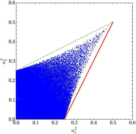
Figure 3: The possible values of $\alpha_{1}^{2}$ and $\alpha_{2}^{2}$. The blue points are values from randomly generated pure product states and the red solid and green dotted lines are the conditions from Eq. (22).

A first possible transformation is the following: One may choose coefficients $x_{i}$ with $\sum_{i}x_{i}=0$ and a small $\varepsilon$ and consider the map $\beta_{i}\mapsto\sqrt{\beta_{i}^{2}+\varepsilon x_{i}}.$ This keeps the normalization $\sum_{i}\beta_{i}^{2}=1$ and it should not increase the value at the maximum. Taking the derivative with respect to $\varepsilon$ and setting afterwards $\varepsilon=0$ we find that at the maximum

$$(\sum_{i}\alpha_{i}\beta_{i})\sum_{k}x_{k}\frac{\alpha_{k}}{\beta_{k}}+\sum_{l}\lambda_{l}x_{l}=0$$ (20)

holds, for any choice of the $x_{i}$. In other words, we can state that at the optimum $\sum_{i}\lambda_{i}x_{i}>0$ is equivalent to $\sum_{i}x_{i}(\alpha_{i}/\beta_{i})<0.$

A second possible transformation affects the $\alpha_{i}$. For the map $\alpha_{i}\mapsto\sqrt{\alpha_{i}^{2}+\varepsilon x_{i}}$ the same argument as above gives that

$$(\sum_{i}\alpha_{i}\beta_{i})\sum_{k}x_{k}\frac{\beta_{k}}{\alpha_{k}}=0$$ (21)

holds at the optimum. Since for the optimal solution there is a finite overlap between $|\psi\rangle$ and $|\phi\rangle$ it follows that $\sum_{k}x_{k}{\beta_{k}}/{\alpha_{k}}=0$. Note that this second transformation might be in conflict with the conditions on the $\alpha_{i}$ coming from the product structure of the vector $|\phi\rangle.$ However, if the coefficients $\alpha_{i}$ are not at the boundary of the allowed values, we can apply it.

As a second step, we have to characterize the possible values of $\alpha_{i}$ in some more detail. More precisely, we claim and will use that (see also Fig. 3)

$$\alpha_{1}^{2}\leq\frac{1}{4}+\frac{\alpha_{2}^{2}}{2}\quad\mbox{ and }\quad\alpha_{2}^{2}\leq\frac{1}{4}+\frac{\alpha_{1}^{2}}{2}.$$ (22)

This follows from the product structure of $|\phi\rangle$ in the following way: It has been shown that the density matrix elements $\varrho_{i,j}$ of any fully separable three-qubit state obey seevinck

$$|\varrho_{1,8}|\leq\sqrt[6]{\varrho_{2,2}\varrho_{3,3}\varrho_{4,4}\varrho_{5,5}\varrho_{6,6}\varrho_{7,7}},$$ (23)

that is, the off-diagonal element $|\varrho_{18}|$ is bounded by a function of the diagonal elements. For the product vector $|\phi\rangle$ we have that $|\varrho_{1,8}|=|\alpha_{1}^{2}-\alpha_{2}^{2}|/2$ and $\varrho_{2,2}=(\alpha_{3}^{2}+\alpha_{4}^{2})/2$ etc., and maximizing the right hand side of Eq. (23) under the normalization $\sum_{i}\alpha_{i}^{2}=1$, one can directly see that Eq. (22) holds. We note that there are further constraints on $\alpha_{1}^{2}$ and $\alpha_{2}^{2}$ from the product structure, but the conditions above together with the positivity of the $\alpha_{1}^{2}$ and $\alpha_{2}^{2}$ represent already the convex hull of all possible values, see also Fig. 3.

After this preliminary considerations we are ready to tackle the main optimization problem of finding the maximum of $\mathcal{F}=(\sum_{i}\alpha_{i}\beta_{i})^{2}+\sum_{i}\lambda_{i}\beta_{i}^{2}$. We first assume that $\lambda_{1}=\mu>0$ and $\lambda_{2}=\nu<0$, the other $\lambda_{i}$ vanish in any case. All the contributions in the zero space of $X$ can be subsumed by single numbers $\alpha_{3}$ and $\beta_{3}$, so without loosing generality we consider only three indices $i=1,2,3.$ We also write the coefficients as vectors $\vec{\alpha}=(\alpha_{1},\alpha_{2},\alpha_{3})$ etc., and denote their scalar product as $\langle\vec{\alpha}|\vec{\beta}\rangle.$ Our aim is to show that the optimal solution of the product vector $|\phi\rangle$ is either given by $\alpha_{1}^{2}=1/4$ and $\alpha_{2}^{2}=0$ (corresponding to the product vector $|\phi\rangle=|+\rangle|+\rangle|+\rangle$ with $|+\rangle=(|0\rangle+|1\rangle)/\sqrt{2}$) or by $\alpha_{1}^{2}=\alpha_{2}^{2}=1/2$ (corresponding to the product vector $|\phi\rangle=|000\rangle$).

As the $\beta_{i}$ have to fulfill only the normalization constraint and $\mu>0$ it is clear that for a given value of $\alpha_{2}^{2}$ the choice of a maximal $\alpha_{1}^{2}$ is optimal. This means that we only have to consider the line $\alpha_{2}^{2}=2\alpha_{1}^{2}-1/2$ with $\alpha_{1}^{2}\in[1/4;1/2]$, being the red solid line in Fig. 3. The endpoints of this line are the possible solutions mentioned above. Note that at this line we have $\alpha_{2}=\sqrt{2\alpha_{1}^{2}-1/2}$ and due to the normalization $\alpha_{3}=\sqrt{3/2-3\alpha_{1}^{2}}$, so everything can be expressed in terms of $\alpha_{1}.$

Let us assume that the solution is not at the endpoints. In the following we will show that under this condition the vector $\vec{\beta}$ is already determined, and the optimal value can be computed. It turns out, however, that the optimum is then the same for all values $\vec{\alpha}$ on the line, so we can also choose the endpoints.

First we can take the derivative in direction of this line. This is done by choosing $\vec{x}=(x_{1},x_{2},x_{3})=(1,2,-3)$ and applying the second transformation from above. It follows that

$$\frac{\beta_{1}}{\alpha_{1}}+\frac{2\beta_{2}}{\alpha_{2}}-\frac{3\beta_{3}}{\alpha_{3}}=0.$$ (24)

So, if we define the vector

$$\vec{v}=\mathcal{N}(\frac{1}{\alpha_{1}},\frac{2}{\alpha_{2}},\frac{-3}{\alpha_{3}}),$$ (25)

where $\mathcal{N}$ denotes a normalization, we have that $\langle\vec{\beta}|\vec{v}\rangle=0$ and $\langle\vec{\alpha}|\vec{v}\rangle=0.$

Then we consider a transformation of the first type from above, affecting the $\beta_{i}$. For a general vector $\vec{x}$ we have that Eq. (20) holds. Especially, we may choose $x_{i}=v_{i}\beta_{i}$, then also $\sum_{i}x_{i}=0$ is satisfied. Then we have for the first term in Eq. (20) $\sum_{k}x_{k}\alpha_{k}/\beta_{k}=\sum_{k}v_{k}\alpha_{k}=0$ and it follows that

$$\beta_{1}\frac{\lambda_{1}}{\alpha_{1}}+2\beta_{2}\frac{\lambda_{2}}{\alpha_{2}}=0.$$ (26)

Equations (24, 26) allow to determine $\vec{\beta}$ up to the normalization. Choosing $\beta_{1}=1$ we find that

$$\beta_{2}=-\frac{\sqrt{2\alpha_{1}^{2}-1/2}\lambda_{1}}{2\alpha_{1}\lambda_{2}},\;\;\;\beta_{3}=\frac{\sqrt{1-2\alpha_{1}^{2}}(\lambda_{2}-\lambda_{1})}{\sqrt{6}\alpha_{1}\lambda_{2}}.$$ (27)

We can insert this solution again in Eq. (20) and use that this holds still for all admissible $\vec{x}=(x_{1},x_{2},-x_{1}-x_{2}).$ This leads to three possible solutions of $\lambda_{2}$ as a function of $\lambda_{1}$. From the conditions $\lambda_{1}>0>\lambda_{2}$ it then follows that

$$\lambda_{2}=\frac{\lambda_{1}^{2}+\lambda_{1}\sqrt{(1-\lambda_{1}+\lambda_{1}^{2})}}{2(\lambda_{1}-1)}$$ (28)

has to hold, with $\lambda_{1}\in[0,1).$ For these values of $\lambda_{1},\lambda_{2},$ however, one directly finds that the function $\mathcal{F}$ does not depend on $\alpha_{1}^{2}$, so $\mathcal{F}$ is constant on the red solid line in Fig. 3. In this way, we have shown that the only relevant points are $\alpha_{1}^{2}=1/4$ and $\alpha_{1}^{2}=1/2.$

Having fixed $\vec{\alpha}$, the optimal $\vec{\beta}$ can directly be determined by looking for the maximal eigenvalue of a $3\times 3$ matrix. In this way one determines the Legendre transform as

$$\hat{E}(\mu,\nu) =\frac{1}{2}\big{[}\mu-1+\sqrt{1+\mu(\mu-1)^{2}}\big{]}$$ (29)

$$\mbox{for }\mu\in(0,1)\mbox{ and }\nu<\frac{\mu^{2}+\mu\sqrt{(1-\mu+\mu^{2})}}{2(\mu-1)},$$

$$\hat{E}(\mu,\nu) =\frac{1}{2}\big{[}\mu+\nu-1+\sqrt{1-(\mu-\nu)^{2}}\big{]}$$ (30)

$$\mbox{for all other values }\mu>0\mbox{ and }\nu<0.$$

This solves the first problem for $\mu>0$ and $\nu<0$, let us shortly discuss what happens for the other possible signs: $\mu<0$ and $\nu>0$ can directly be solved as above. For the case $\mu>0,\nu>0$ the solution is obviously given by choosing $\alpha_{1}^{2}=\alpha_{2}^{2}=1/2$, leading to the formula (30) again. Finally, if $\mu<0,\nu<0$ the optimum is attained by choosing $\alpha_{1}^{2}=\alpha_{2}^{2}=0$ and $\alpha_{3}^{2}=1$. But then, $\hat{E}(\mu,\nu)=0$ does not depend on $\mu$ and $\nu$ at all, so this case has no physical relevance.

It remains to compute the geometric measure from the Legendre transform and the values of the fidelity. We have to optimize

$$E(f^{+},f^{-})=\sup_{\mu,\nu}\{\mu f^{+}+\nu f^{-}-\hat{E}(\mu,\nu)\}$$ (31)

for the functions given in Eqs. (29, 30). Let us consider the parameters as in Eq. (29) first. In this case, $\hat{E}(\mu,\nu)$ does not depend on $\nu$ at all, so it is clear to take $\nu$ as large as possible, since $f^{-}\geq 0$. So we have to choose $\nu=[{\mu^{2}+\mu\sqrt{(1-\mu+\mu^{2})}}]/[{2(\mu-1)}].$ If $\hat{E}$ is given by Eq. (30), we can consider a transformation $\mu\mapsto\mu-\varepsilon$ and $\nu\mapsto\nu-\varepsilon$. This increases $(-\hat{E})$ by $\varepsilon$, on the other hand, the term $\mu f^{+}+\nu f^{-}$ decreases less, since $f^{+}+f^{-}\leq 1.$ Consequently, it is optimal to take $\varepsilon$ as large as possible, which means that the optimum is attained again at the boundary, where $\nu=[{\mu^{2}+\mu\sqrt{(1-\mu+\mu^{2})}}]/[{2(\mu-1)}].$ Note that at this boundary the condition $\mu\in(0,1)$ is automatically fulfilled.

In summary, the computation of $E(f^{+},f^{-})$ can be reduced to an optimization over the single parameter $\mu,$ namely

$$E_{G}^{(3)}(f^{+},f^{-})=\!\!\max_{\mu\in[0,1]}\frac{1}{2}\big{[}1+\mu(2f^{+}-1)-\sqrt{\alpha}+\frac{f^{-}\mu(\mu+\sqrt{\alpha})}{\mu-1}\big{]},$$ (32)

where we used the abbreviation $\alpha=1-\mu+\mu^{2}.$ This is the statement of Observation 1. Clearly, the formula (32) gives the value $E_{G}^{(3)}$ for the case $f^{+}\geq f^{-}$ only, since for this case $\mu>0>\nu$ is the relevant choice of parameters. For the other case one has to exchange the values of $f^{+}$ and $f^{-}$. $\hfill\Box$

VII.2 The optimal decomposition

Here we find the optimal decomposition for GHZ-symmetric three-qubit states at the lower cathetus where $f^{-}=0.$ Let us denote these states by $\varrho(f^{+})$. The entries of these density matrices are given by $\varrho_{1,1}=\varrho_{8,8}=\varrho_{1,8}=\varrho_{8,1}=f^{+}/2$, the other entries on the diagonal are $\varrho_{2,2}=\varrho_{3,3}=...=\varrho_{7,7}=(1-f^{+})/6$ and all other entries vanish. For the decomposition, we consider first the following four vectors:

$$|\psi_{1}\rangle =\alpha(|000\rangle+|111\rangle)$$

$$+\beta(|001\rangle+|010\rangle+|011\rangle+|100\rangle+|101\rangle+|110\rangle),$$

$$|\psi_{2}\rangle =\sigma_{z}\otimes\sigma_{z}\otimes\openone|\psi_{1}\rangle,$$

$$|\psi_{3}\rangle =\sigma_{z}\otimes\openone\otimes\sigma_{z}|\psi_{1}\rangle,$$

$$|\psi_{4}\rangle =\openone\otimes\sigma_{z}\otimes\sigma_{z}|\psi_{1}\rangle,$$ (33)

with $\alpha=\sqrt{f^{+}/2}$ and $\beta=\sqrt{(1-2\alpha^{2})/6}=\sqrt{(1-f^{+})/6}.$ The density matrix $|\psi_{1}\rangle\!\langle\psi_{1}|$ has the same entries on the diagonal as $\varrho(f^{+})$ and the entries $\varrho_{1,8}$ and $\varrho_{8,1}$ also coincide. The symmetrized density matrix $X_{1}=(1/4)\sum_{k=1}^{4}|\psi_{k}\rangle\!\langle\psi_{k}|$ fulfills the same properties, but has only elements on the diagonal and anti-diagonal.

So far, the values of $X_{1}$ on the anti-diagonal other than $\varrho_{1,8}$ and $\varrho_{8,1}$ do not vanish, contrary to the values of $\varrho(f^{+})$. So we consider vectors of the type

$$|\xi(\phi_{1},\phi_{2},\phi_{3})\rangle=e^{i\phi_{1}\sigma_{z}}\otimes e^{i\phi_{2}\sigma_{z}}\otimes e^{i\phi_{3}\sigma_{z}}|\psi_{1}\rangle$$ (34)

with the constraint $\phi_{1}+\phi_{2}+\phi_{3}=0.$ As explained before, this is also a symmetry of the states in the considered family. We first consider

$$|\psi_{5}\rangle=|\xi(\pi/4,\pi/4,-\pi/2)\rangle$$ (35)

and define $|\psi_{6}\rangle,|\psi_{7}\rangle,|\psi_{8}\rangle$ via a symmetrization as in Eq. (33). The matrix $X_{5}=(1/4)\sum_{k=5}^{8}|\psi_{k}\rangle\!\langle\psi_{k}|$ is similar to $X_{1}$, but the entry $\varrho_{2,8}$ has a different sign, and $\varrho_{3,7}$ and $\varrho_{4,5}$ have the phase $-i$. Adding the vectors

$$|\psi_{9}\rangle=|\xi(-\pi/4,-\pi/4,\pi/2)\rangle$$ (36)

with the symmetrizations $|\psi_{10}\rangle,|\psi_{11}\rangle,|\psi_{12}\rangle$ and $X_{9}=(1/4)\sum_{k=9}^{12}|\psi_{k}\rangle\!\langle\psi_{k}|$ we find that $Y=X_{1}/2+X_{5}/4+X_{9}/4$ has, apart from $\varrho_{3,7}$ and $\varrho_{4,5}$ all the entries as $\varrho(f^{+})$, also $\varrho_{2,8}$ is vanishing. Repeating this procedure with

$$|\psi_{13}\rangle = |\xi(\pi/4,-\pi/2,\pi/4,)\rangle,$$

$$|\psi_{17}\rangle = |\xi(-\pi/4,\pi/2,-\pi/4)\rangle,$$

$$|\psi_{21}\rangle = |\xi(-\pi/2,\pi/4,\pi/4)\rangle,$$

$$|\psi_{25}\rangle = |\xi(\pi/2,-\pi/4,-\pi/4,)\rangle$$ (37)

and the respective symmetrizations we arrive at a decomposition of $\varrho(f^{+})$ into 28 pure states.

It remains to show that this is the optimal decomposition. By taking the overlap with the product state $|\Phi\rangle=|+\rangle|+\rangle|+\rangle$ the geometric measure of $|\psi_{1}\rangle$ is bounded by

$$E(|\psi_{1}\rangle) \leq 1-\frac{1}{8}(2\alpha+6\beta)^{2}$$ (38)

$$= \frac{1}{4}(1+2f^{+}-2\sqrt{3}\sqrt{f^{+}(1-f^{+})})$$

which coincides with formula Eq. (7) if the fidelity $f^{+}\leq 3/4$. This also proves that in this regime the state $|\Phi\rangle$ was indeed the closest product state to $|\psi_{1}\rangle.$ For fidelities larger than that one can directly check that $|\Phi\rangle$ is not the closest state anymore, computing the geometric measure leads then to a function that is not convex in $f^{+}$. Since the geometric measure must be convex, however, the optimal decomposition is then not given by the decomposition into the $|\psi_{1}\rangle$ anymore. Instead, the optimal decomposition is for $f^{+}>3/4$ just given by

$$\varrho(f^{+})=(1-p)\varrho(f^{+}=3/4)+p|GHZ^{+}\rangle\!\langle GHZ^{+}|$$ (39)

with $p=4f^{+}-3.$ Of course, $\varrho(f^{+}=3/4)$ should be understood here as a placeholder of its optimal decomposition into 28 pure states. This reproduces the second (linear) part of Eq. (7). $\hfill\Box$

VII.3 Proof of Observation 2

In order to show this Observation let us first consider full separability of an $N$-qubit state (that is, $k=N$) and discuss what parts of the previous proof of Observation 1 require modification. The first modification is Eq. (23) which has to be replaced by the generalization

$$|\varrho_{1,2^{N}}|\leq(\varrho_{2,2}\varrho_{3,3}\cdot...\cdot\varrho_{2^{N}-1,2^{N}-1})^{\frac{1}{2^{N}-2}},$$ (40)

The corresponding generalization of Eq. (22) reads

$$\alpha_{1}^{2}\leq\frac{1}{2^{N-1}}\big{[}1+(2^{N-1}-2){\alpha_{2}^{2}}\big{]},$$

$$\alpha_{2}^{2}\leq\frac{1}{2^{N-1}}\big{[}1+(2^{N-1}-2){\alpha_{1}^{2}}\big{]}.$$ (41)

In this way, the deltoid in Fig. 3 becomes smaller. This time, the state $|\phi\rangle=|+\rangle^{\otimes N}$ corresponds to the corner $\alpha_{1}^{2}=1/(2^{N-2})$ and $\alpha_{2}^{2}=0$ and the state $|\phi\rangle=|0\rangle^{\otimes N}$ corresponds to $\alpha_{1}^{2}=\alpha_{2}^{2}=1/2.$

With this modification, one can first show as before that only the corners of the modified deltoid are relevant. Then, one has to diagonalize again $3\times 3$ matrices to arrive at similar expressions to Eqs. (29, 30). In fact, Eq. (30) does not change, while Eq. (29) reads

$$\hat{E}(\mu,\nu) =\frac{1}{2}\big{[}\mu-1+\sqrt{(\mu-1)^{2}+2^{3-N}\mu}\big{]}.$$ (42)

With this one can argue as before that only the line where the two types of the Legendre transform coincide is relevant. This leads to Eq. (10).

Finally, we have to discuss what happens if we consider the geometric measure for $k$ separability of an $N$ qubit state, if $k<N.$ This can be understood as follows: Let us assume that we have a pure $k$-separable state, which has to be separable for a fixed partition. To be explicit, consider the three-separable six-qubit state $|\Psi\rangle=|\phi_{1}\rangle\otimes|\phi_{23}\rangle\otimes|\phi_{456}\rangle$. We claim that this state obeys the conditions of Eq. (41) with $N$ set to $k$. Indeed, by projecting the possibly entangled groups of $\ell$ qubits on the space $\Pi_{\ell}=|00...0\rangle\!\langle 00...0|+|11...1\rangle\!\langle 11...1|$ and identifying the logical qubits $|0\rangle_{L}=|00...0\rangle$ and $|1\rangle_{L}=|11...1\rangle$ we arrive at a state which is effectively a fully separable $k$-qubit state. In our example, we have to apply $\openone\otimes\Pi_{2}\otimes\Pi_{3}$ to $|\Psi\rangle$ to arrive at this state. The fidelities of the GHZ states $|GHZ^{\pm}\rangle$ do not change, as the GHZ states are invariant under the projections. It follows that any pure $k$-separable $N$-qubit state obeys the conditions of Eq. (41) with $N$ set to $k$. In addition, one can also reach the corners of the deltoid by appropriate $N$-qubit $k$-separable states. From this point, the proof can proceed as before and one arrives at Eq. (10). $\hfill\Box$

VII.4 Proof of Observation 3

In this case, the deltoid from Fig. 3 becomes a square. When computing the eigenvalues of the matrices before Eqs. (29, 30) it is then clear that one of the possible solutions is larger than the other. So the Legendre transform reduces to

$$\hat{E}(\mu,\nu) =\frac{1}{2}\big{[}\mu-1+\sqrt{1+\mu^{2}}\big{]}.$$ (43)

In the final optimization, one has to set $\nu=0.$ The remaining optimization over $\mu\geq 0$ can be carried out analytically, and one finds that if $f^{+}\geq 1/2$ the geometric measure is given by

$$E(f^{+},f^{-})=\frac{1}{2}-\sqrt{f^{+}(f^{+}-1)}.$$ (44)

The analogous formula holds if $f^{-}\geq 1/2$. For the other cases the geometric measure vanishes, as the state is biseparable. $\hfill\Box$

References

- (1) R. Horodecki, P. Horodecki, M. Horodecki, and K. Horodecki, Rev. Mod. Phys. 81, 865 (2009), O. Gühne and G. Tóth, Phys. Rep. 474, 1 (2009).
- (2) M. B. Plenio and S. Virmani, Quantum Inf. Comput. 7, 1 (2007); C. Eltschka and J. Siewert, J. Phys. A: Math. Theor. 47, 424005 (2014).
- (3) T.-C. Wei and P.M. Goldbart, Phys. Rev. A 68, 042307 (2003), see also A. Shimony, Ann. N.Y. Acad. Sci. 755, 675 (1995).
- (4) M. Blasone, F. Dell’Anno, S. De Siena, and F. Illuminati Phys. Rev. A 77, 062304 (2008); A. Sen De and U. Sen, Phys. Rev. A 81, 012308 (2010).
- (5) M. Hayashi et al., D. Markham, M. Murao, M. Owari, and S. Virmani, Phys. Rev. Lett. 96, 040501 (2006).
- (6) T.-C. Wei, D. Das, S. Mukhopadyay, S. Vishveshwara, and P.M. Goldbart, Phys. Rev. A 71, 060305(R) (2005); R. Orus, Phys. Rev. Lett. 100, 130502 (2008); H. Shekhar Dhar, A. Sen De, and U. Sen, Phys. Rev. Lett. 111, 070501 (2013).
- (7) A. Streltsov, H. Kampermann, and D. Bruß, New J. Phys. 12, 123004 (2010).
- (8) O. Gühne, F. Bodoky, and M. Blaauboer, Phys. Rev. A 78, 060301 (2008).
- (9) S. Bagchi, A. Misra, A. Sen(De), and U. Sen, poster at the IWQI 2012 workshop in Allahabad, India (2012).
- (10) W. K. Wootters, Phys. Rev. Lett. 80, 2245 (1998); A. Uhlmann, Phys. Rev. A 62 032307 (2000); Entropy 12, 1799 (2010).
- (11) C. Eltschka and J. Siewert, Phys. Rev. Lett. 108, 020502 (2012).
- (12) B. M. Terhal and K. G. H. Vollbrecht, Phys. Rev. Lett. 85, 2625 (2000); K. G. H. Vollbrecht and R. F. Werner, Phys. Rev. A 64, 062307 (2001); P. Rungta and C. M. Caves, Phys. Rev. A 67, 012307 (2003); R. Lohmayer, A. Osterloh, J. Siewert, and A. Uhlmann, Phys. Rev. Lett. 97, 260502 (2006).
- (13) G Tóth, T. Moroder, and O. Gühne, arXiv:1409.3806.
- (14) K. Horodecki, M. Horodecki, and P. Horodecki, Quantum Inf. Comput. 10, 901 (2010).
- (15) C. Eltschka and J. Siewert, Phys. Rev. A 89, 022312 (2014).
- (16) O. Gühne, M. Reimpell, and R.F. Werner, Phys. Rev. Lett. 98, 110502 (2007); J. Eisert, F. Brandão, and K. Audenaert, New J. Phys. 9, 46 (2007).
- (17) We strongly recommend the use of a computer algebra package at this point.
- (18) W. Dür and J. I. Cirac, J. Phys. A: Math. Gen. 34, 6837 (2001).
- (19) A. Kay, Phys. Rev. A 83, 020303(R) (2011).
- (20) J. Martin, O. Giraud, P. A. Braun, D. Braun, and T. Bastin, Phys. Rev. A 81, 062347 (2010).
- (21) R. Jozsa, J. Mod. Optics 41, 2315 (1994).
- (22) O. Gühne, M. Reimpell, and R.F. Werner, Phys. Rev. A. 77, 052317 (2008).
- (23) O. Gühne and M. Seevinck, New J. Phys. 12, 053002 (2010).