Transmission phase lapse in the non-Hermitian Aharonov–Bohm interferometer near the spectral singularity

Abstract

We study the effect of $\mathcal{PT}$-symmetric imaginary potentials embedded in the two arms of an Aharonov-Bohm interferometer on the transmission phase by finding an exact solution for a concrete tight-binding system. It is observed that the spectral singularity always occurs at $k=\pm\pi/2$ for a wide range of fluxes and imaginary potentials. Critical behavior associated with the physics of the spectral singularity is also investigated. It is demonstrated that the quasi-spectral singularity corresponds to a transmission maximum and the transmission phase jumps abruptly by $\pi$ when the system is swept through this point. Moreover, We find that there exists a pulse-like phase lapse when the imaginary potential approaches the boundary value of the spectral singularity.

I Introduction

Both the phase and the magnitude of a wavefunction are two important quantities associated with quantum phenomena in nature. A direct application is that the phase and magnitude of transmission can contain information regarding the scattering center. For probability-based detection, we can look back to the much earlier investigation of atomic structure, which led to the development of the Rutherford model of the atom E. Rutherford11 and eventually to the Bohr model. Now, the continued development of technology makes it possible to experimentally investigate the transmission phase, which contains information complementary to the transmission probability A. Yacoby95 ; Yang Ji00 ; Yang Ji02 ; M. Sigrist04 ; M. Avinun-Kalish05 ; M. Zaffalon08 . These measurements of the transmission phase mainly focus on the so-called phase lapse phenomenon, which refers to an abrupt jump in the transmission phase through a quantum dot between transmission peaks G. Hackenbroich01 .

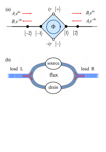
Figure 1: (Color online) Schematic illustration of configuration of concerned non-Hermitian AB interferometer. (a) It consists of a Hermitian tight-binding square with an AB flux $\Phi$ and two semi-infinite chains as the waveguides connecting to the scattering center. The non-Hermiticity of the scattering center arises from the $\mathcal{PT}$ symmetric potentials $\pm i\gamma$ with respect to the axis along the leads. It is shown that the transmission phase is sensitive to the flux when the system is near the spectral singularity. (b) The model setup represents an open AB interferometer with a source and drain embedded in the two arms, which can be phenomenologically described by the type of tight-binding model in (a). The flux breaks the balance between the source and drain and may result in new transport behavior.

A non-Hermitian Hamiltonian can possess peculiar features that have no counterpart in a closed Hermitian system. A typical example is non-reciprocal dynamics, which has been observed in experiments Observe . Especially, previous work LXQ indicates that the combination of magnetic field and non-Hermitian potential appears to have an unexpected effect on particle transport behavior. The discovery of non-Hermitian Hamiltonians with parity-time symmetry, which have a real spectrum Bender , has fundamentally boosted the research on the complex extension of quantum mechanics Ann ; JMP1 ; JPA1 ; JPA2 ; PRL1 ; JMP2 ; JMP3 ; JMP4 ; JPA3 ; JPA4 ; JPA5 . Recently, the concept of spectral singularity of a non-Hermitian system has attracted considerable attention PRA1 ; PRB1 ; Ali3 ; PRA3 ; JMP5 ; PRD1 ; PRA4 ; PRA5 ; PRA6 , motivated by the pioneering work of Mostafazadeh on the possible physical relevance of the said concept PRL3 . Most previous works focus on non-Hermitian systems with $\mathcal{PT}$-symmetry potentials PRA2 ; JPA6 ; Ali3 ; PRA13 ; prd2 ; prd3 ; prd4 ; prd5 ; prd6 ; prd7 ; prd8 , non-Hermitian hopping amplitude PRA14 ; ZXZ ; S. Longhi14 , and imaginary particle-particle interaction strength LGR .

In this study, we investigate the property of a non-Hermitian Aharonov-Bohm (AB) interferometer with $\mathcal{PT}$-symmetric imaginary potentials embedded in its two arms. We find that the spectral singularity with $k=\pm\pi/2$ exists for the system in a wide range of fluxes and imaginary potentials. It is demonstrated that the quasi-spectral singularity corresponds to a transmission maximum, and the transmission phase jumps abruptly by $\pi$ when the system is swept through this point. Furthermore, a pulse-like phase lapse exists when the imaginary potential approaches the boundary value of the spectral singularity. This model can also suggest a scheme for the realization of non-Hermitian imaginary hopping integral via on-site imaginary potential. These findings can be exploited to detect regions of criticality without having to undergo the spectral singularity and to enhance interferometer sensitivity.

The remainder of this paper is organized as follows. In Section II, we present the model setup and the solutions. In Section III, the spectral singularity of the Hamiltonian is examined. In Section IV, we study transmission lapses near the spectral singularity. Finally, we present a summary and discussion in Section V.

II Model and solutions

The non-Hermitian interferometer shown in Fig. 1 is described by the Hamiltonian

$$H = H_{\mathrm{0}}+H_{\mathrm{c}}$$ (1)

$$H_{\mathrm{0}} = \sum_{j=1}^{N}\left(\left|j\right\rangle\left\langle j+1\right|+\left|-j\right\rangle\left\langle-j-1\right|+\mathrm{H.c.}\right),$$ (2)

$$H_{\mathrm{c}} = \frac{1}{\sqrt{2}}\sum_{\sigma=\pm}\left(e^{-i\sigma\phi}\left|-1\right\rangle+e^{i\sigma\phi}\left|1\right\rangle\right)\left\langle\sigma\right|+\mathrm{H.c.}$$ (3)

$$+i\gamma\sum_{\sigma=\pm}\sigma\left|\sigma\right\rangle\left\langle\sigma\right|,$$

which is a single-particle tight-binding model, where $\left|j\right\rangle$ denotes the site-state $j$. We consider the dimensionless hopping integral $J=1$ for simplicity. $H_{\mathrm{0}}$ represents the two leads, while $H_{\mathrm{c}}$ is a non-Hermitian scattering center with an AB flux $\Phi=4\phi$ enclosed by the two arms. The non-Hermiticity of the scattering center arises from the $\mathcal{PT}$-symmetric potentials $\pm i\gamma$ with respect to the axis along the leads. This phenomenon can be employed to phenomenologically depict an open interferometer, a multi-terminal device G. Hackenbroich01 . For a tight-binding lattice network, equivalence between the imaginary potential and the input (output) lead is proposed L. Jin10 ; JL . In another case, the imaginary potential was added to an interferometer to introduce dephasing C. Benjamin02 .

For the present model, we note that it has $\mathcal{PF}$-symmetry,

$$\mathcal{\hat{P}\hat{F}}H\left(\mathcal{\hat{P}\hat{F}}\right)^{-1}=H,$$ (4)

where the parity and flux flipping operators are

$$\mathcal{\hat{P}} : \left|j\right\rangle\rightarrow\left|-j\right\rangle,$$ (5)

$$\mathcal{\hat{F}} : \mathcal{\hat{F}}H\left(\phi\right)\mathcal{\hat{F}}^{-1}=H\left(-\phi\right).$$ (6)

For the flux-free case $\phi=0$, the system is $\mathcal{PT}$-symmetric about the axis along the leads and $\mathcal{P}$-symmetric about the axis through the locations of the imaginary potentials. A previous work L. Jin12 shows that it is a probability-preserved system owing to balance between $i\gamma$ and $-i\gamma$. It is presumable that the flux may break such a balance and result in new transport behavior.

Based on the Bethe ansatz method, the solution of the Schrodinger equation

$$H\left|\psi_{k}\right\rangle=\varepsilon_{k}\left|\psi_{k}\right\rangle$$ (7)

takes the form

$$\left\langle j\right.\left|\psi_{k}\right\rangle=\left\{\begin{array}[]{cc}A_{-}e^{ikj}+B_{-}e^{-ikj},&\left(j\leqslant-1\right)\\ B_{+}e^{ikj}+A_{+}e^{-ikj},&\left(j\geqslant 1\right)\end{array}\right..$$ (8)

Eq. (7) results in $\varepsilon_{k}=2\cos k$ and two-component spinor equation

$$\chi\left(\begin{array}[]{c}B_{-}\\ B_{+}\end{array}\right)=\left|\chi\right|e^{i\theta\overrightarrow{n}\cdot\overrightarrow{\sigma}}\left(\begin{array}[]{c}A_{-}\\ A_{+}\end{array}\right)$$ (9)

where $\overrightarrow{n}=\left(n_{x},n_{y},0\right)$, $\overrightarrow{\sigma}=\left(\sigma_{x},\sigma_{y},\sigma_{z}\right)$ is a Pauli matrix. When $\chi=0$, Eq. (9) is not useful. We will discuss this later. Here the parameters are defined as

$$\left\{\begin{array}[]{c}\left|\chi\right|e^{i\theta}=\left|\eta\right|^{2}-\xi^{+}\xi^{-}+i2\text{Im}\left(\eta\right)\sqrt{\xi^{+}\xi^{-}},\\ n_{x}=\left(\xi^{+}+\xi^{-}\right)/\sqrt{4\xi^{+}\xi^{-}},\\ n_{y}=i\left(\xi^{+}-\xi^{-}\right)/\sqrt{4\xi^{+}\xi^{-}},\end{array}\right.,$$ (10)

and

$$\left\{\begin{array}[]{c}\chi=\left[\xi^{+}\xi^{-}-\left(\eta^{\ast}\right)^{2}\right]e^{2ik},\\ \eta=\left(e^{2ik}+1+\gamma^{2}\right)e^{ik},\\ \xi^{\pm}=2\cos k\cos\left(2\phi\right)\pm\gamma\sin\left(2\phi\right),\end{array}\right..$$ (11)

A straightforward implication of Eq. (9) is that it represents the rotation operation of a two-component spinor. The direction of the rotating axis $\overrightarrow{n}$ and angle $\theta$ could be complex. In general, a given pair of arbitrary constants $A_{\pm}$ can generate a pair of constants $B_{\pm}$, both of which together construct the eigenfunction $\left|\psi_{k}\right\rangle$. This indicates that the energy levels are doubly degenerate. According to the theory of pseudo-Hermitian quantum mechanics A. Mostafazadeh04 , a complete biorthogonal system requires the construction of the eigenfunctions of $H^{{\dagger}}$.

In parallel, we can perform the same procedure for the eigenfunction of the Hamiltonian $H^{{\dagger}}$. Similarly, we have the Schrodinger equation

$$H^{{\dagger}}\left|\overline{\psi}_{k}\right\rangle=\varepsilon_{k}\left|\overline{\psi}_{k}\right\rangle$$ (12)

and the eigenfunction

$$\left\langle j\right.\left|\overline{\psi}_{k}\right\rangle=\left\{\begin{array}[]{cc}\overline{A}_{-}e^{ikj}+\overline{B}_{-}e^{-ikj},&\left(j\leqslant-1\right)\\ \overline{B}_{+}e^{ikj}+\overline{A}_{+}e^{-ikj},&\left(j\geqslant 1\right)\end{array}\right..$$ (13)

The corresponding rotation equation of the two-component spinor reads

$$\chi\left(\begin{array}[]{c}\overline{B}_{-}\\ \overline{B}_{+}\end{array}\right)=\left|\chi\right|e^{i\theta\overrightarrow{\overline{n}}\cdot\overrightarrow{\sigma}}\left(\begin{array}[]{c}\overline{A}_{-}\\ \overline{A}_{+}\end{array}\right),$$ (14)

where only the unitary vector needs to be redefined as $\overrightarrow{\overline{n}}=\left(n_{x},-n_{y},0\right)$.

To construct the two degenerate eigenstates from a pair of arbitrary constants $A_{\pm}$, it is beneficial to investigate the complete set of two-component spinors. Taking the Hermitian conjugate of Eq. (14) and multiplying it by Eq. (9), we have

$$\left|\chi\right|^{2}\left(\overline{B}_{-}^{\ast},\overline{B}_{+}^{\ast}\right)\left(\begin{array}[]{c}B_{-}\\ B_{+}\end{array}\right)$$ (17)

$$= \left(\overline{A}_{-}^{\ast},\overline{A}_{+}^{\ast}\right)\left|\chi\right|^{2}e^{-i\theta^{\ast}\overrightarrow{\overline{n}}^{\ast}\cdot\overrightarrow{\sigma}}e^{i\theta\overrightarrow{n}\cdot\overrightarrow{\sigma}}\left(\begin{array}[]{c}A_{-}\\ A_{+}\end{array}\right)$$ (20)

$$= \left|\chi\right|^{2}\left(\overline{A}_{-}^{\ast},\overline{A}_{+}^{\ast}\right)\left(\begin{array}[]{c}A_{-}\\ A_{+}\end{array}\right).$$ (23)

It indicates that the orthonormal relationship between $\left(\overline{A}_{-},\overline{A}_{+}\right)$ and $\left(A_{-},A_{+}\right)$ can be transferred to that between $\left(\overline{B}_{-},\overline{B}_{+}\right)$ and $\left(B_{-},B_{+}\right)$. This allows us to construct an entire biorthogonal system based on an orthonormal set of two-component spinors. Here, we povide an example by taking

$$\left(\begin{array}[]{c}\overline{A}_{-}\\ \overline{A}_{+}\end{array}\right)=\left(\begin{array}[]{c}A_{-}\\ A_{+}\end{array}\right)=\left(\begin{array}[]{c}\alpha_{-}\\ \alpha_{+}\end{array}\right),\text{ }\left(\begin{array}[]{c}-\alpha_{+}^{\ast}\\ \alpha_{-}^{\ast}\end{array}\right),$$ (24)

where $\left|\alpha_{+}\right|^{2}+\left|\alpha_{-}\right|^{2}=1$. The corresponding spinors $\left(\overline{B}_{-},\overline{B}_{+}\right)$ and $\left(B_{-},B_{+}\right)$ are obtained immediately. Then, for $\chi\neq 0$, we have two degenerate eigenfunctions of $H$

$$\left\langle j\right.\left|\psi_{k}^{1}\right\rangle=\frac{C_{1}}{\sqrt{N}}\left\{\begin{array}[]{cc}\alpha_{-}e^{ikj}+\beta_{-}^{1}e^{-ikj},&\left(j\leqslant-1\right)\\ \alpha_{+}e^{-ikj}+\beta_{+}^{1}e^{ikj},&\left(j\geqslant 1\right)\end{array}\right.,$$ (25)

and

$$\left\langle j\right.\left|\psi_{k}^{2}\right\rangle=\frac{C_{2}}{\sqrt{N}}\left\{\begin{array}[]{cc}-\alpha_{+}^{\ast}e^{ikj}+\beta_{-}^{2}e^{-ikj},&\left(j\leqslant-1\right)\\ \alpha_{-}^{\ast}e^{-ikj}+\beta_{+}^{2}e^{ikj},&\left(j\geqslant 1\right)\end{array}\right.,$$ (26)

where $N$ is the system size. Here, the amplitudes

$$\beta_{\pm}^{1} = \frac{1}{\chi}\left[\left(\left|\eta\right|^{2}-\xi^{+}\xi^{-}\right)\alpha_{\pm}+i2\text{Im}\left(\eta\right)\xi^{\mp}\alpha_{\mp}\right],$$ (27)

$$\beta_{\pm}^{2} = \frac{1}{\chi}\left[\pm\left(\left|\eta\right|^{2}-\xi^{+}\xi^{-}\right)\alpha_{\mp}^{\ast}\mp i2\text{Im}\left(\eta\right)\xi^{\mp}\alpha_{\pm}^{\ast}\right],$$ (28)

can be complex numbers and

$$C_{1}=\frac{\left|\chi\right|}{\sqrt{2\left|\chi\right|^{2}+\Lambda_{++}}}\text{, }C_{2}=\frac{\left|\chi\right|}{\sqrt{2\left|\chi\right|^{2}+\Lambda_{--}}},$$ (29)

are real numbers, where

$$\Lambda_{\sigma\sigma^{\prime}}=4\text{Im}\left(\eta\right)\left(\xi^{+}-\xi^{-}\right)[\text{Im}\left(\eta\right)\left(\xi^{+}\left|\alpha_{\sigma^{\prime}}\right|^{2}-\xi^{-}\left|\alpha_{-\sigma^{\prime}}\right|^{2}\right)$$

$$\sigma\left(\left|\eta\right|^{2}-\xi^{+}\xi^{-}\right)\text{Im}\left(\alpha_{-}\alpha_{+}^{\ast}\right)],\left(\sigma,\sigma^{\prime}=\pm\right).$$ (30)

Accordingly, the eigenfunctions of $H^{{\dagger}}$ can be expressed as

$$\left\langle j\right.\left|\overline{\psi}_{k}^{1}\right\rangle=\frac{\overline{C}_{1}}{\sqrt{N}}\left\{\begin{array}[]{cc}\alpha_{-}e^{ikj}+\overline{\beta}_{-}^{1}e^{-ikj},&\left(j\leqslant-1\right)\\ \alpha_{+}e^{-ikj}+\overline{\beta}_{+}^{1}e^{ikj},&\left(j\geqslant 1\right)\end{array}\right.,$$ (31)

and

$$\left\langle j\right.\left|\overline{\psi}_{k}^{2}\right\rangle=\frac{\overline{C}_{2}}{\sqrt{N}}\left\{\begin{array}[]{cc}-\alpha_{+}^{\ast}e^{ikj}+\overline{\beta}_{-}^{2}e^{-ikj},&\left(j\leqslant-1\right)\\ \alpha_{-}^{\ast}e^{-ikj}+\overline{\beta}_{+}^{2}e^{ikj},&\left(j\geqslant 1\right)\end{array}\right.,$$ (32)

where $\overline{\beta}_{\pm}^{\lambda}\left(\phi\right)=\beta_{\pm}^{\lambda}\left(-\phi\right)$, and real number $\overline{C}_{\lambda}\left(\phi\right)=C_{\lambda}\left(-\phi\right)$, $\left(\lambda=1,2\right)$, or

$$\overline{C}_{1}=\frac{\left|\chi\right|}{\sqrt{2\left|\chi\right|^{2}+\Lambda_{+-}}}\text{, }\overline{C}_{2}=\frac{\left|\chi\right|}{\sqrt{2\left|\chi\right|^{2}+\Lambda_{-+}}}\text{.}$$ (33)

It is easy to check that $\left\langle\psi_{k}^{\lambda}\right.\left|\psi_{k}^{\lambda}\right\rangle=1$. However, generally, $\left\langle\psi_{k}^{\lambda}\right.\left|\psi_{k}^{\lambda^{\prime}}\right\rangle\neq 0$ for $\lambda\neq\lambda^{\prime}$, unless the parameters are taken special value, e.g., $\gamma=0$ or $\sin\left(2\phi\right)=0$. In contrast, we have

$$\left\langle\overline{\psi}_{k}^{\lambda}\right.\left|\psi_{k}^{\lambda^{\prime}}\right\rangle=2\overline{C}_{\lambda}C_{\lambda}\delta_{\lambda\lambda^{\prime}}=\left|\chi\right|^{2}\mathcal{G}\left(\left|\chi\right|\right)\delta_{\lambda\lambda^{\prime}},$$ (34)

where one can see that $\mathcal{G}\left(\left|\chi\right|\right)$ is a nonzero bounded real function. It indicates that one can always normalize the amplitudes $\overline{C}_{\lambda}$ and $C_{\lambda}$ to achieve a complete biorthogonal system.

Before we end this section, we would like to point out that: (i) It is not helpful to choose eigenfunctions within each degeneracy subspace by using the $\mathcal{PF}$-symmetry because $\mathcal{\hat{F}}$ is not a Hermitian operator. (ii) In the limit $\chi\rightarrow 0$, the biorthogonal relationship in Eq. (34) tends to collapse, which implies the emergence of the spectral singularity.

III Spectral singularity

In this section, we will demonstrate the existence of spectral singularity of the system and explore the feature of the solution at the critical point. We start by considering the eigenfunctions of the system at the point $\left(k_{c},\phi_{c},\gamma_{c}\right)$ with $k_{c}=\pm\pi/2$ and

$$\sin^{2}\left(2\phi_{c}\right)=\gamma_{c}^{2},$$ (35)

which lead to $\chi=0$. In this study, we only consider the non-Hermitian case with $\gamma>0$. Thus, Eqs. (7) and (12) can be rewritten as

$$2\gamma_{c}^{4}\left(I\mp\sigma_{y}\right)\{\left(\begin{array}[]{c}A_{-}\\ A_{+}\end{array}\right),\left(\begin{array}[]{c}\overline{B}_{-}\\ \overline{B}_{+}\end{array}\right)\} = 0,$$ (40)

$$2\gamma_{c}^{4}\left(I\pm\sigma_{y}\right)\{\left(\begin{array}[]{c}\overline{A}_{-}\\ \overline{A}_{+}\end{array}\right),\left(\begin{array}[]{c}B_{-}\\ B_{+}\end{array}\right)\} = 0.$$ (45)

The solutions of these equations are $A_{+}=\pm iA_{-}$, $\overline{A}_{+}=\mp i\overline{A}_{-}$, and $B_{+}=\mp iB_{-}$, $\overline{B}_{+}=\pm i\overline{B}_{-}$, which admit the eigenfunction of $H$ at the spectral singularity

$$\left\langle j\right.\left|\psi_{\pm\pi/2}^{c}\right\rangle=\frac{1}{\sqrt{2N}}\left\{\begin{array}[]{cc}e^{\pm i\frac{\pi}{2}j},&\left(j\leqslant-1\right)\\ \pm ie^{\mp i\frac{\pi}{2}j},&\left(j\geqslant 1\right)\end{array}\right.,$$ (46)

where $\left|\psi_{\pm\pi/2}^{c}\right\rangle=\left|\psi_{\pm\pi/2}^{1}\right\rangle=\left|\psi_{\mp\pi/2}^{2}\right\rangle$. And the corresponding eigenfunction of $H^{\dagger}$ is

$$\left\langle j\right.\left|\overline{\psi}_{\pm\pi/2}^{c}\right\rangle=\frac{1}{\sqrt{2N}}\left\{\begin{array}[]{cc}e^{\pm i\frac{\pi}{2}j},&\left(j\leqslant-1\right)\\ \mp ie^{\mp i\frac{\pi}{2}j},&\left(j\geqslant 1\right)\end{array}\right..$$ (47)

Similarly, $\left|\overline{\psi}_{\pm\pi/2}^{c}\right\rangle=\left|\overline{\psi}_{\pm\pi/2}^{1}\right\rangle=\left|\overline{\psi}_{\mp\pi/2}^{2}\right\rangle$. The physics of the solutions is clear that $\left|\psi_{-\pi/2}^{c}\right\rangle$ describes self-sustained emission from the scattering center (lasering), while $\left|\psi_{\pi/2}^{c}\right\rangle$ represents reflectionless absorption of two incident plane waves (anti-lasering).

It can be readily checked whether

$$\left\langle\overline{\psi}_{\pm\pi/2}^{c}\right.\left|\psi_{\pm\pi/2}^{c}\right\rangle=\left\langle\overline{\psi}_{\pm\pi/2}^{c}\right.\left|\psi_{\mp\pi/2}^{c}\right\rangle=0,$$ (48)

which indicates that the complete biorthogonality of the eigenfunctions of $H$ and $H^{{\dagger}}$ is destroyed at the points $\chi=0$. This so-called spectral singularity has peculiar features for the present concrete system: (i) The spectral singularity always occurs at the fixed $k$, which is independent of the values of $\gamma$ and $\phi$, whenever $\gamma$ is within the range $\left[-1,1\right]$. (ii) The transfer matrix $M$, which is defined as

$$\left(\begin{array}[]{c}B_{+}\\ A_{+}\end{array}\right)=M\left(\begin{array}[]{c}A_{-}\\ B_{-}\end{array}\right)$$ (49)

has different property for the present scattering center. In fact, for Eq. (9) we have

$$\left(\eta-\eta^{\ast}\right)\xi^{+}\chi\left(\begin{array}[]{c}B_{+}\\ A_{+}\end{array}\right)=\widetilde{M}\left(\begin{array}[]{c}A_{-}\\ B_{-}\end{array}\right),$$ (50)

where the modified transfer matrix is

$$\widetilde{M}=\left(\begin{array}[]{cc}-\left|\chi\right|^{2}&\chi\left(\left|\eta\right|^{2}-\xi^{+}\xi^{-}\right)\\ -\chi\left(\left|\eta\right|^{2}-\xi^{+}\xi^{-}\right)&\chi^{2}\end{array}\right).$$ (51)

For $\left(\eta-\eta^{\ast}\right)\xi^{+}\chi\neq 0$, the determinant of the transfer matrix is

$$\det M=\frac{\xi^{-}}{\xi^{+}}=\frac{2\cos k\cos\left(2\phi\right)-\gamma\sin\left(2\phi\right)}{2\cos k\cos\left(2\phi\right)+\gamma\sin\left(2\phi\right)},$$ (52)

which is a function of $\left(k,\phi,\gamma\right)$. We find that whenever $k=\pm\pi/2$ and $4\phi\neq 2n\pi$, we always have $\det M=-1$, which differs from the conclusion, $\det M=1$, in Refs. Ali1 ; Ali2 for systems without flux. This implies that a scattering center subjected to a magnetic field can have some special features. For the case of $\chi=0$, which corresponds to the spectral singularity, we have

$$M=\left(\begin{array}[]{cc}0&-i\\ i&0\end{array}\right),$$ (53)

from the solutions of Eq. (45). This is in accordance with the conclusion in Ali1 ; Ali2 that a signature of the spectral singularity is $M_{22}=0$.

To exemplify the application of the present model, we will show that the AB interferometer can be employed to realize a non-Hermitian imaginary hopping integral in the tight-binding model. It has been reported that a non-Hermitian center with imaginary hopping can be accessed by suitable longitudinal modulations of gain/loss and propagation constants in evanescently-coupled optical waveguide arrays, and it serves as a key building block for realizing invisible defects in non-Hermitian tight-binding lattices S. Longhi10 .

We begin with a simple case with $\phi=\pi/4$. Taking the following linear transformation

$$\left\{\begin{array}[]{c}\left|j\right\rangle=\underline{\left|j\right\rangle}\text{, }j\leqslant-1\\ \left|+\right\rangle=\frac{1}{\sqrt{2}}e^{-i\pi/4}(\underline{\left|+\right\rangle}+\underline{\left|-\right\rangle})\text{,}\\ \left|-\right\rangle=\frac{1}{\sqrt{2}}e^{i\pi/4}(\underline{\left|+\right\rangle}-\underline{\left|-\right\rangle})\text{,}\\ \left|j\right\rangle=-i\underline{\left|j\right\rangle}\text{, }j\geqslant 1\text{,}\end{array}\right.$$ (54)

the original Hamiltonian (1) can be written as

$$H_{\pi/4} = \sum_{j=1}^{N}(\underline{\left|j\right\rangle}\underline{\left\langle j+1\right|}+\underline{\left|-j\right\rangle}\underline{\left\langle-j-1\right|})$$ (55)

$$+(\underline{\left|-1\right\rangle}\underline{\left\langle+\right|}+\underline{\left|1\right\rangle}\underline{\left\langle-\right|})+\mathrm{H.c.}$$

$$+i\gamma(\underline{\left|+\right\rangle}\underline{\left\langle-\right|}+\underline{\left|-\right\rangle}\underline{\left\langle+\right|}),$$

which reduces the AB ring to a non-Hermitian imaginary hopping dimer. According to the above analysis, $H_{\pi/4}$ has a spectral singularity at $k=\pm\pi/2$ when $\gamma=1$.

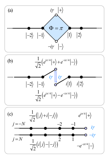
Figure 2: (Color online) Schematic illustration of exemplified system. (a) Non-Hermitian scattering center configuration with $\phi=\pi/4$, which consists of two on-site imaginary potentials $i\gamma$ and $-i\gamma$. (b) The equivalent Hamiltonian $H_{\pi/4}$ in Eq. (55), which is obtained via linear transformation of Eq. (54). It represents a system with a non-Hermitian imaginary hopping dimer, which has the hopping integral $i\gamma$. (c) The equivalent Hamiltonian $H_{\pi/4}$ in Eq. (57) is obtained via the two linear transformations of Eqs. (54) and (56). It is shown that the original Hamiltonian can be mapped to two separated Hamiltonians $H_{\pm}$, describing semi-infinite chains with ending imaginary potentials $\pm i\gamma$.

Taking the following linear transformation

$$\left\{\begin{array}[]{c}\underline{\left|j\right\rangle}=\frac{1}{\sqrt{2}}(\overline{\left|j\right\rangle}-\overline{\left|-j\right\rangle})\text{, }j\leqslant-1\\ \underline{\left|+\right\rangle}=\frac{1}{\sqrt{2}}(\overline{\left|+\right\rangle}-\overline{\left|-\right\rangle})\text{,}\\ \underline{\left|-\right\rangle}=\frac{1}{\sqrt{2}}(\overline{\left|+\right\rangle}+\overline{\left|-\right\rangle})\text{,}\\ \underline{\left|j\right\rangle}=\frac{1}{\sqrt{2}}(\overline{\left|j\right\rangle}+\overline{\left|-j\right\rangle})\text{, }j\geqslant 1\end{array}\right.$$ (56)

the Hamiltonian $H_{\pi/4}$ is decomposed into two separate parts

$$H_{\pi/4} = H_{+}+H_{-},$$ (57)

$$H_{+} = \sum_{j=-N}^{-1}\overline{\left|j\right\rangle}\overline{\left\langle j+1\right|}+\overline{\left|-1\right\rangle}\overline{\left\langle+\right|}+\mathrm{H.c.}$$ (58)

$$+i\gamma\overline{\left|+\right\rangle}\overline{\left\langle+\right|},$$

$$H_{-} = \sum_{j=1}^{N}\overline{\left|j\right\rangle}\overline{\left\langle j+1\right|}+\overline{\left|1\right\rangle}\overline{\left\langle-\right|}+\mathrm{H.c.}-i\gamma\overline{\left|-\right\rangle}\overline{\left\langle-\right|}.$$ (59)

The physics of the models clearly describe semi-infinite chains with ending imaginary potentials $\pm i\gamma$. Such systems have been studied systematically in a previous work PRA14 , in which the result was the solution given in Eq. (46). Therefore, the dynamic behaviors, self-sustained emission, and reflectionless absorption of wavepackets, can emerge in the system $H_{\pi/4}$ as well.

IV Transmission phase lapse

In this section, we investigate another physical relevance of the spectral singularity. We begin with the scattering problem of the AB interferometer, which should shed some light on the dynamics of wavepackets in the critical region. The eigenfunctions of the incident wave from left and right can be obtained by taking

$$\left(\begin{array}[]{c}A_{-}\\ A_{+}\end{array}\right)=\left(\begin{array}[]{c}1\\ 0\end{array}\right)\text{, }\left(\begin{array}[]{c}0\\ 1\end{array}\right).$$ (60)

We have two degenerate eigenfunctions of $H$

$$\left\langle j\right.\left|\psi_{k}^{\mathrm{L}}\right\rangle=\left\{\begin{array}[]{cc}e^{ikj}+r_{\mathrm{L}}e^{-ikj},&\left(j\leqslant-1\right)\\ t_{\mathrm{L}}e^{ikj},&\left(j\geqslant 1\right)\end{array}\right.,$$ (61)

and

$$\left\langle j\right.\left|\psi_{k}^{\mathrm{R}}\right\rangle=\left\{\begin{array}[]{cc}e^{-ikj}+r_{\mathrm{R}}e^{ikj},&\left(j\geqslant 1\right)\\ t_{\mathrm{R}}e^{-ikj},&\left(j\leqslant-1\right)\end{array}\right..$$ (62)

The transmission and reflection amplitudes $t_{\mathrm{L,R}}$ and $r_{\mathrm{L,R}}$ can be obtained from the corresponding $B_{\pm}$. These amplitudes obey the relations

$$r_{\mathrm{R}}\left(\phi\right)=r_{\mathrm{L}}\left(-\phi\right)=r_{\mathrm{L}}\text{, }t_{\mathrm{R}}\left(\phi\right)=t_{\mathrm{L}}\left(-\phi\right),$$ (63)

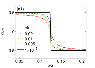
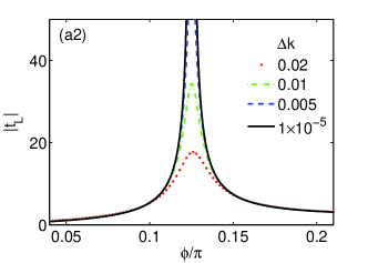
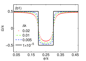
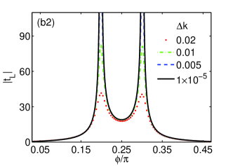
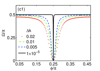
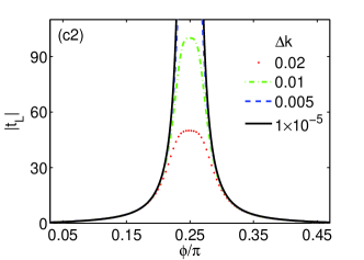
Figure 3: (Color online) Plots of transmission amplitudes as functions of flux near spectral singularity, which demonstrate two types of lapse of transmission phase for various $k=k_{c}+\Delta k$. The phase and magnitude of $t_{\mathrm{L}}$ in Eq. (65) are plotted for (a) $\gamma=0.707$, (b) $\gamma=0.949$, (c) $\gamma=1.00$. The plot shows that the profiles of the transmission phase and the magnitude of $t_{\mathrm{L}}$ are in agreement with our analysis based on the Eq. (66).

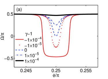
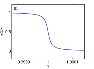
Figure 4: (Color online) Crossover from $\pi$ lapse to zero lapse for system with $\gamma$ around $1$. (a) Plots of transmission phases for $k=\pi/2+10^{-5}$ as functions of the flux near the spectral singularity, which show the pulse-like lapse with different heights. (b) The maximal phase shifts for $k=\pi/2+10^{-5}$ as a function of $\gamma$, as obtained from $t_{\mathrm{L}}$ in Eq. (65). The profiles of the transmission phase as functions of $\phi$ and $\gamma$ are in agreement with our analysis based on Eq. (66).

owing to $\mathcal{PF}$-symmetry and can be written in the explicit form

$$r_{\mathrm{L}}=\frac{\left|e^{2ik}+1+\gamma^{2}\right|^{2}-\left[4\cos^{2}k\cos^{2}\left(2\phi\right)-\gamma^{2}\sin^{2}\left(2\phi\right)\right]}{e^{2ik}\left[4\cos^{2}k\cos^{2}\left(2\phi\right)-\gamma^{2}\sin^{2}\left(2\phi\right)\right]-\left(e^{-2ik}+1+\gamma^{2}\right)^{2}},$$ (64)

and

$$t_{\mathrm{L}}=\frac{\left[e^{ik}\left(e^{2ik}+1+\gamma^{2}\right)-\mathrm{C.c.}\right]\left(2\cos k\cos\left(2\phi\right)-\gamma\sin\left(2\phi\right)\right)}{e^{2ik}\left[4\cos^{2}k\cos^{2}\left(2\phi\right)-\gamma^{2}\sin^{2}\left(2\phi\right)\right]-\left(e^{-2ik}+1+\gamma^{2}\right)^{2}}.$$ (65)

In the vicinity of the spectral singularity $\left(k_{c},\phi_{c},\gamma_{c}\right)$, we have

$$t_{\mathrm{L}}\approx\frac{\gamma_{c}^{2}}{\left|\rho\right|}\mathrm{sign}\left[\gamma_{c}\sin\left(2\phi_{c}\right)\right]e^{i\Omega},$$ (66)

where

$$\left\{\begin{array}[]{c}\rho=\sin\left(4\phi_{c}\right)\left(\phi-\phi_{c}\right)+2\cos\left(4\phi_{c}\right)\left(\phi-\phi_{c}\right)^{2}\\ -\left(\gamma-\gamma_{c}\right)+i\left(2-\gamma_{c}^{2}\right)\left(k-k_{c}\right),\\ \Omega=\mathrm{Arg}\left(\rho\right)-\frac{\pi}{2},\end{array}\right..$$ (67)

The term $\left(\phi-\phi_{c}\right)^{2}$ is retained for the case of very small $\sin\left(4\phi_{c}\right)$. This approximate expression in Eq. (66) indicates that the transmission phase exhibits following features.

(i) In the case of $0<\gamma<1$, there always exists spectral singularities, for instance, at the point $\phi_{c}$ (or $\pi/2-\phi_{c}$), $k_{c}=\pi/2$ and $\gamma_{c}=\gamma$. We now consider the transmission behavior of $k\sim k_{c}$, $\phi$ varying in the vicinity of $\phi_{c}$. When $\gamma$ is not close to $0$ and $1$ such that the term $\left(\phi-\phi_{c}\right)$ is dominant in the real part of $\rho$, the magnitude of $\rho$ reaches a minimum, while its real part switches its sign as $\phi$ passes the point $\phi_{c}$. According to Eq. (66), these events lead to the magnitude of $t_{\mathrm{L}}$ reaching a maximum at $\phi=\phi_{c}$, while the phase $\Omega$ jumps by $\pi$ in the case of $\left|\phi-\phi_{c}\right|\gg\left|\left(2-\gamma_{c}^{2}\right)\left(k-k_{c}\right)/\sin\left(4\phi_{c}\right)\right|$. We can see that the phase shift becomes very abrupt when $k$ is close to $k_{c}$. Then in the limit case, lapse of the transmission phase is from $\pi/2$ to $-\pi/2$. Similarly, a lapse from $-\pi/2$ to $\pi/2$ should occur near the point $\pi/2-\phi_{c}$. This implies two succeeding abrupt shifts when the two points $\phi_{c}$ and $\pi/2-\phi_{c}$ are close to each other. Actually, when $\gamma$ is close to $1$, from Eq. (35), we have $\phi_{c}\approx\pi/4$. According to Eq. (66), the magnitude of $t_{\mathrm{L}}$ reaches a minimum at $\phi=n\pi/4$, but maxima at $\phi=\phi_{c}$, $\pi/2-\phi_{c}$. The transmission phase can exhibit a pulse-like shift of height $\pi$, i.e., a lapse from $\pi/2$ to $-\pi/2$ to $\pi/2$. We will see from the following analysis that as $\gamma_{c}$ increases to $1$, the pulse height decreases.

(ii) In the case of $\gamma>1$, there is no singularity. When $\gamma$ is not close to $1$ such that the term $\left(\gamma-1\right)$ is dominant in the real part of $\rho$, there is no lapse of the transmission phase as $\phi$ passes the point $\phi_{c}=\pi/4$. It is interesting to see what happens to the crossover from (i) to (ii). To this end, we consider the following case.

(iii) $\gamma=1$. For this case, we have $\phi_{c}=\pi/4$, the term of $\left(\phi-\phi_{c}\right)^{2}$ being dominant in the real part of $\rho$. The magnitude of $t_{\mathrm{L}}$ reaches a maximum at $\phi=\pi/4$, while the transmission phase experiences two succeeding abrupt $\pi/2$ shifts as $\phi$ varies, i.e., from $\pi/2$ to $0$ to $\pi/2$, similar to a pulse of height $\pi/2$. This indicates crossover of the transmission phase lapse from $\pi$ to zero.

To demonstrate the above analysis, we plot the phase and magnitude from Eq. (65) for several types of cases in Fig. 3. The figure shows that our analysis is in accordance with the exact expression $t_{\mathrm{L}}$ when the system approaches the spectral singularity. Moreover, we simulated the crossover from case (i) to (ii), as shown in Fig. 4. First, for various values of $\gamma$ around $1$, we plot the phase $\Omega\left(\phi\right)$ as a function of $\phi$. Secondly, we plot the maximal phase shift, which is defined as $\Delta\Omega=\mathrm{Max}\left[\Omega\left(\phi\right)-\Omega\left(\pi/4\right)\right]$, as a function of $\gamma$. The numerical results clearly show that the transmission phase lapse is a good indicator of the transition between systems with and without spectral singularity.

V Summary and discussion

In summary, we studied the non-Hermitian AB interferometer. On the basis of the exact solution of a concrete tight-binding system, it is found that there are fixed spectral singularities at $k=\pm\pi/2$ for a wide range of fluxes and imaginary potentials. The critical behavior associated with the physics of the spectral singularity exhibits two types of lapses of the transmission phases, from $\pi/2$ to $-\pi/2$ and from $\pi/2$ to $-\pi/2$ to $\pi/2$. These phenomena can be exploited as a tool to detect the regions of criticality without undergoing the spectral singularity and enhance interferometer sensitivity. In addition, the concrete example also suggested a scheme for realizing non-Hermitian imaginary hopping dimer with the aid of on-site imaginary potential. This appears to imply that the combination of $\mathcal{PT}$-symmetric non-Hermitian potential and magnetic flux is crucial for such a phenomenon. Finally, this approach can be extended to more generalized systems such as interferometers with longer arms and complex potential as $\pm i\gamma\rightarrow\pm\left(V+i\gamma\right)$, in which the spectral singularity should not be fixed.

References

(1) E. Rutherford, Philos. Mag. 6, 21 (1911).
(2) A. Yacoby, M. Heiblum, D. Mahalu, and H. Shtrikman,
Phys. Rev. Lett. 74, 4047 (1995).
(3) Y. Ji, M. Heiblum, D. Sprinzak, D. Mahalu, and H.
Shtrikman, Science 290, 779 (2000).
(4) Y. Ji, M. Heiblum, and H. Shtrikman, Phys. Rev. Lett.
88, 076601 (2002).
(5) M. Sigrist, A. Fuhrer, T. Ihn, K. Ensslin, S. E.
Ulloa, W. Wegscheider, and M. Bichler, Phys. Rev. Lett. 93, 066802
(2004).
(6) M. Avinun-Kalish, M. Heiblum, O. Zarchin, D.
Mahalu, and V. Umansky, Nature (London) 436, 529 (2005).
(7) M. Zaffalon, A. Bid, M. Heiblum, D. Mahalu, and V.
Umansky, Phys. Rev. Lett. 100, 226601 (2008).
(8) G. Hackenbroich, Phys. Rep. 343, 463
(2001).
(9) A. Guo, G. J. Salamo, D. Duchesne, R. Morandotti, M.
Volatier-Ravat, V. Aimez, G. A. Siviloglou, and D. N. Christodoulides, Phys.
Rev. Lett. 103, 093902 (2009).
(10) X. Q. Li, X. Z. Zhang, G. Zhang, and Z. Song, arXiv:1409.0420.
(11) C. M. Bender and S. Boettcher, Phys. Rev. Lett. 80, 5243 (1998).
(12) F. G. Scholtz, H. B. Geyer, and F. J. W. Hahne, Ann. Phys.
(NY) 213, 74 (1992).
(13) C. M. Bender, S. Boettcher, and P. N. Meisinger, J. Math.
Phys. 40, 2201 (1999).
(14) C. M. Bender, D. C. Brody, and H. F. Jones, Phys. Rev. Lett.
89, 270401 (2002).
(15) P. Dorey, C. Dunning, and R. Tateo, J. Phys. A 34,
L391 (2001).
(16) P. Dorey, C. Dunning, and R. Tateo, J. Phys. A 34,
5679 (2001).
(17) A. Mostafazadeh, J. Math. Phys. 43, 205 (2002).
(18) A. Mostafazadeh, J. Math. Phys. 43, 2814 (2002).
(19) A. Mostafazadeh, J. Math. Phys. 43, 3944 (2002).
(20) A. Mostafazadeh and A. Batal, J. Phys. A 36, 7081
(2003).
(21) A. Mostafazadeh and A. Batal, J. Phys. A 37, 11645
(2004).
(22) H. F. Jones, J. Phys. A 38, 1741 (2005).
(23) A. Mostafazadeh, Phys. Rev. A 80, 032711 (2009).
(24) A. Mostafazadeh, Phys. Rev. A 84, 023809 (2011).
(25) A. Mostafazadeh, Phys. Rev. Lett. 110. 260402 (2013).
(26) A. Mostafazadeh and M. Sarisaman, Phys. Rev. A 87,
063834 (2013).
(27) A. Mostafazadeh, and M. Sarisaman, Phys. Rev. A 88,
033810 (2013).
(28) S. Longhi, Phys. Rev. B 80, 165125 (2009).
(29) A. A. Andrianov, F. Cannata, and A. V. Sokolov, J. Math.
Phys. (N.Y.) 51, 052104 (2010).
(30) F. Correa and M. S. Plyushchay, Phys. Rev. D 86,
085028 (2012).
(31) L. Chaos-Cador and G. García-Calderón Phys. Rev. A
87, 042114 (2013).
(32) A. Mostafazadeh, Phys. Rev. Lett. 102, 220402 (2009).
(33) H. F. Jones, Phys. Rev. D 76, 125003 (2007).
(34) H. F. Jones, Phys. Rev. D 78, 065032 (2008).
(35) M. Znojil, Phys. Rev. D 78, 025026 (2008).
(36) M. Znojil, Phys. Rev. D 80, 045009 (2009).
(37) M. Znojil, Phys. Rev. D 80, 045022 (2009).
(38) M. Znojil, Phys. Rev. D 80, 105004 (2009).
(39) C. M. Bender and P. D. Mannheim, Phys. Rev. D 78,
025022 (2008).
(40) S. Longhi, Phys. Rev. A 81, 022102 (2010).
(41) A. Ghatak, J. A. Nathan, B. P. Mandal, and Z. Ahmed, J. Phys.
A: Math. Theor. 45, 465305 (2012).
(42) A. Mostafazadeh, Phys. Rev. A 87, 063838 (2013).
(43) X. Z. Zhang, L. Jin, and Z. Song, Phys. Rev. A 87,
042118 (2013).
(44) X. Z. Zhang and Z. Song, Ann. Phys. 339, 109 (2013).
(45) S. Longhi, EPL 106, 34001 (2014).
(46) G. R. Li, X. Z. Zhang, and Z. Song, Ann. Phys. 349,
288 (2014).
(47) L. Jin and Z. Song, Phys. Rev. A 81, 032109
(2010).
(48) L. Jin and Z. Song, Phys. Rev. A 80, 052107 (2009).
(49) C. Benjamin and A. M. Jayannavar, Phys. Rev. B
65, 153309 (2002).
(50) L. Jin and Z. Song, Phys. Rev. A 85, 012111
(2012).
(51) A. Mostafazadeh and A. Batal, J. Phys. A: Math.
Gen. 37, 11645 (2004).
(52) A. Mostafazadeh, J. Phys. A: Math. Gen. 39 13495
(2006).
(53) A. Mostafazadeh and H. Mehri-Dehnavi, J. Phys. A: Math.
Theor. 42, 125303 (2009).