Optimal switching for pairs trading rule:
a viscosity solutions approach

Abstract

This paper studies the problem of determining the optimal cut-off for pairs trading rules. We consider two correlated assets whose spread is modelled by a mean-reverting process with stochastic volatility, and the optimal pair trading rule is formulated as an optimal switching problem between three regimes: flat position (no holding stocks), long one short the other and short one long the other. A fixed commission cost is charged with each transaction. We use a viscosity solutions approach to prove the existence and the explicit characterization of cut-off points via the resolution of quasi-algebraic equations. We illustrate our results by numerical simulations.

Keywords: pairs trading, optimal switching, mean-reverting process, viscosity solutions.

MSC Classification: 60G40, 49L25.

JEL Classification: C61, G11.

1 Introduction

Pairs trading consists of taking simultaneously a long position in one of the assets $A$ and $B$, and a short position in the other, in order to eliminate the market beta risk, and be exposed only to relative market movements determined by the spread. A brief history and discussion of pairs trading can be found in Ehrman [7], Vidyamurthy [18] and Elliott, Van der Hoek and Malcom [9]. The main aim of this paper is to rationale mathematically these rules and find optimal cutoffs, by means of a stochastic control approach.

Pairs trading problem has been studied by stochastic control approach in the recent years. Mudchanatongsuk, Primbs and Wong [13] consider self-financing portfolio strategy for pairs trading, model the log-relationship between a pair of stock prices by an Ornstein-Uhlenbeck process and use this to formulate a portfolio optimization and obtain the optimal solution to this control problem in closed form via the corresponding Hamilton-Jacobi-Bellman (HJB) equation. They only allow positions that are short one stock and long the other, in equal dollar amounts. Tourin and Yan [17] study the same problem, but allow strategies with arbitrary amounts in each stock. On the other hand, instead of using self-financing strategies, one can focus on determining the optimal cut-offs, i.e. the boundaries of the trading regions in which one should trade when the spread lies in. Such problem is closely related to optimal buy-sell rule in trading mean reverting asset. Zhang and Zhang [19] studied optimal buy-sell rule, where they model the underlying asset price by an Ornstein-Uhlenbeck process and consider an optimal trading rule determined by two regimes: buy and sell. These regimes are defined by two threshold levels, and a fixed commission cost is charged with each transaction. They use classical verification approach to find the value function as solution to the associated HJB equations (quasi-variational inequalities), and the optimal thresholds are obtained by smooth-fit technique. The same problem is studied in Kong’s PhD thesis [10], but he considers trading rules with three aspects: buying, selling and shorting. Song and Zhang [16] use the same approach for determining optimal pairs trading thresholds, where they model the difference of the stock prices $A$ and $B$ by an Ornstein-Uhlenbeck process and consider an optimal pairs trading rule determined by two regimes: long $A$ short $B$ and flat position (no holding stocks). Leung and Li [11] studied the optimal timing to open or close the position subject to transaction costs, and the effect of Stop-loss level under the Ornstein-Uhlenbeck (OU) model. They directly construct the value functions instead of using variational inequalities approach, by characterizing the value functions as the smallest concave majorant of reward function.

In this paper, we consider a pairs trading problem as in Song and Zhang [16], but differ in our model setting and resolution method. We consider two correlated assets whose spread is modelled by a more general mean-reverting process with stochastic volatility, and the optimal pairs trading rule is based on optimal switching between three regimes: flat position (no holding stocks), long one short the other and vice-versa. A fixed commission cost is charged with each transaction. We use a viscosity solutions approach to solve our optimal switching problem. Actually, by combining viscosity solutions approach, smooth fit properties and uniqueness result for viscosity solutions proved in Pham, Ly Vath and Zhou [15], we are able to derive directly the structure of the switching regions, and thus the form of our value functions. This contrasts with the classical verification approach where the structure of the solution should be guessed ad-hoc, and one has to check that it satisfies indeed the corresponding HJB equation, which is not trivial in this context of optimal switching with more than two regimes.

The paper is organized as follows. We formulate in Section 2 the pairs trading as an optimal switching problem with three regimes. In Section 3, we state the system of variational inequalities satisfied by the value functions in the viscosity sense and the definition of pairs trading regimes. In Section 4, we state some useful properties on the switching regions, derive the form of value functions, and obtain optimal cutoff points by relying on the smooth-fit properties of value functions. In Section 5, we illustrate our results by numerical examples.

2 Pair trading problem

Let us consider the spread $X$ between two correlated assets, say $A$ and $B$ modelled by a mean-reverting process with boundaries $\ell_{-}$ $\in$ $\{-\infty,0\}$, and $\ell_{+}$ $=$ $\infty$:

$$dX_{t} = \mu(L-X_{t})dt+\sigma(X_{t})dW_{t},$$ (2.1)

where $W$ is a standard Brownian motion on $(\Omega,{\cal F},\mathbb{F}=({\cal F}_{t})_{t\geq 0},\mathbb{P})$, $\mu$ $>$ $0$ and $L$ $\geq$ $0$ are positive constants, $\sigma$ is a Lipschitz function on $(\ell_{-},\ell_{+})$, satisfying the nondegeneracy condition $\sigma$ $>$ $0$. The SDE (2.1) admits then a unique strong solution, given an initial condition $X_{0}$ $=$ $x$ $\in$ $(\ell_{-},\ell_{+})$, denoted $X^{x}$. We assume that $\ell_{+}$ $=$ $\infty$ is a natural boundary, $\ell_{-}$ $=$ $-\infty$ is a natural boundary, and $\ell_{-}$ $=$ $0$ is non attainable. The main examples are the Ornstein-Uhlenbeck (OU in short) process or the inhomogenous geometric Brownian motion (IGBM), as studied in detail in the next sections.

Suppose that the investor starts with a flat position in both assets. When the spread widens far from the equilibrium point, she naturally opens her trade by buying the underpriced asset, and selling the overpriced one. Next, if the spread narrows, she closes her trades, thus generating a profit. Such trading rules are quite popular in practice among hedge funds managers with cutoff values determined empirically by descriptive statistics. The main aim of this paper is to rationale mathematically these rules and find optimal cutoffs, by means of a stochastic control approach. More precisely, we formulate the pairs trading problem as an optimal switching problem with three regimes. Let $\{-1,0,1\}$ be the set of regimes where $i$ $=$ $0$ corresponds to a flat position (no stock holding), $i$ $=$ $1$ denotes a long position in the spread corresponding to a purchase of $A$ and a sale of $B$, while $i$ $=$ $-1$ is a short position in $X$ (i.e. sell $A$ and buy $B$). At any time, the investor can decide to open her trade by switching from regime $i$ $=$ $0$ to $i$ $=$ $-1$ (open to sell) or $i$ $=$ $1$ (open to buy). Moreover, when the investor is in a long ($i$ $=$ $1$) or short position ($i$ $=$ $-1$), she can decide to close her position by switching to regime $i$ $=$ $0$. We also assume that it is not possible for the investor to switch directly from regime $i$ $=$ $-1$ to $i$ $=$ $1$, and vice-versa, without first closing her position. The trading strategies of the investor are modelled by a switching control $\alpha$ $=$ $(\tau_{n},\iota_{n})_{n\geq 0}$ where $(\tau_{n})_{n}$ is a nondecreasing sequence of stopping times representing the trading times, with $\tau_{n}$ $\rightarrow$ $\infty$ a.s. when $n$ goes to infinity, and $\iota_{n}$ valued in $\{-1,0,1\}$, ${\cal F}_{\tau_{n}}$-measurable, represents the position regime decided at $\tau_{n}$ until the next trading time. By misuse of notations, we denote by $\alpha_{t}$ the value of the regime at any time $t$:

$$\alpha_{t} = \iota_{0}{\bf 1}_{\{0\leq t<\tau_{0}\}}+\sum_{n\geq 0}\iota_{n}{\bf 1}_{\{\tau_{n}\leq t<\tau_{n+1}\}},\;\;\;t\geq 0,$$

which also represents the inventory value in the spread at any time. We denote by $g_{ij}(x)$ the trading gain when switching from a position $i$ to $j$, $i,j$ $\in$ $\{-1,0,1\}$, $j$ $\neq$ $i$, for a spread value $x$. The switching gain functions are given by:

$$g_{{}_{01}}(x)\;=\;g_{{}_{-10}}(x) = -(x+\varepsilon)$$

$$g_{{}_{0-1}}(x)\;=\;g_{{}_{10}}(x) = x-\varepsilon,$$

where $\varepsilon$ $>$ $0$ is a fixed transaction fee paid at each trading time. Notice that we do not consider the functions $g_{{}_{-11}}$ and $g_{{}_{11}}$ since it is not possible to switch from regime $i$ $=$ $-1$ to $i$ $=$ $1$ and vice-versa. By misuse of notations, we also set $g(x,i,j)$ $=$ $g_{{}_{ij}}(x)$.

Given an initial spread value $X_{0}$ $=$ $x$, the expected reward over an infinite horizon associated to a switching trading strategy $\alpha$ $=$ $(\tau_{n},\iota_{n})_{n\geq 0}$ is given by the gain functional:

$$J(x,\alpha) = \mathbb{E}\Big{[}\sum_{n\geq 1}e^{-\rho\tau_{n}}g(X_{\tau_{n}}^{x},\alpha_{\tau_{n}^{-}},\alpha_{\tau_{n}})-\lambda\int_{0}^{\infty}e^{-\rho t}|\alpha_{t}|dt\Big{]}.$$

The first (discrete sum) term corresponds to the (discounted with discount factor $\rho$ $>$ $0$) cumulated gain of the investor by using pairs trading strategies, while the last integral term reduces the inventory risk, by penalizing with a factor $\lambda$ $\geq$ $0$, the holding of assets during the trading time interval.

For $i$ $=$ $0,-1,1$, let $v_{i}$ denote the value functions with initial positions $i$ when maximizing over switching trading strategies the gain functional, that is

$$v_{i}(x) = \sup_{\alpha\in{\cal A}_{i}}J(x,\alpha),\;\;\;\;\;x\in(\ell_{-},\infty),\;i=0,-1,1,$$

where ${\cal A}_{i}$ denotes the set of switching controls $\alpha$ $=$ $(\tau_{n},\iota_{n})_{n\geq 0}$ with initial position $\alpha_{0^{-}}$ $=$ $i$, i.e. $\tau_{0}$ $=$ $0$, $\iota_{0}$ $=$ $i$. The impossibility of switching directly from regime $i$ $=$ $\pm 1$ to $\mp 1$ is formalized by restricting the strategy of position $i=\pm 1$: if $\alpha\in{\cal A}_{{}_{1}}$ or $\alpha\in{\cal A}_{{}_{-1}}$ then $\iota_{{}_{1}}$ $=$ $0$ for ensuring that the investor has to close first her position before opening a new one.

3 PDE characterization

Throughout the paper, we denote by ${\cal L}$ the infinitesimal generator of the diffusion process $X$, i.e.

$${\cal L}\varphi(x) = \mu(L-x)\varphi^{\prime}(x)+\frac{1}{2}\sigma^{2}(x)\varphi^{\prime\prime}(x).$$

The ordinary differential equation of second order

$$\rho\phi-{\cal L}\phi = 0,$$ (3.1)

has two linearly independent positive solutions. These solutions are uniquely determined (up to a multiplication), if we require one of them to be strictly increasing, and the other to be strictly decreasing. We shall denote by $\psi_{+}$ the increasing solution, and by $\psi_{-}$ the decreasing solution. They are called fundamental solutions of (3.1), and any other solution can be expressed as their linear combination. Since $\ell_{+}$ $=$ $\infty$ is a natural boundary, and $\ell_{-}$ $\in$ $\{-\infty,0\}$ is either a natural or non attainable boundary, we have:

$$\psi_{+}(\infty)\;=\;\psi_{-}(\ell_{-})\;=\;\infty, \psi_{-}(\infty)\;=\;0.$$ (3.2)

We shall also assume that

$$\lim_{x\rightarrow\ell_{-}}\frac{x}{\psi_{-}(x)}\;=\;0, \lim_{x\rightarrow\infty}\frac{x}{\psi_{+}(x)}\;=\;0.$$ (3.3)

Canonical examples
Our two basic examples in finance for $X$ satisfying the above assumptions are

• Ornstein-Uhlenbeck (OU) process:

  $$dX_{t} = -\mu X_{t}dt+\sigma dW_{t},$$ (3.4)

  with $\mu$, $\sigma$ positive constants. In this case, $\ell_{+}$ $=$ $\infty$, $\ell_{-}$ $=$ $-\infty$ are natural boundaries, the two fundamental solutions to (3.1) are given by

  $$\psi_{+}(x)=\int_{0}^{\infty}t^{\frac{\rho}{\mu}-1}\exp\big{(}-\frac{t^{2}}{2}+\frac{\sqrt{2\mu}}{\sigma}xt\big{)}dt, \psi_{-}(x)=\int_{0}^{\infty}t^{\frac{\rho}{\mu}-1}\exp\big{(}-\frac{t^{2}}{2}-\frac{\sqrt{2\mu}}{\sigma}xt\big{)}dt,$$

  and it is easily checked that condition (3.3) is satisfied.

• Inhomogeneous Geometric Brownian Motion (IGBM):

  $$dX_{t}=\mu(L-X_{t})dt+\sigma X_{t}dW_{t},\;\;\;X_{{}_{0}}>0,$$ (3.5)

  where $\mu$, $L$ and $\sigma$ are positive constants. In this case, $\ell_{+}$ $=$ $\infty$ is a natural boundary, $\ell_{-}$ $=$ $0$ is a non attainable boundary, and the two fundamental solutions to (3.1) are given by

  $$\psi_{+}(x)=x^{-a}U(a,b,\frac{c}{x}), \psi_{-}(x)=x^{-a}M(a,b,\frac{c}{x}).$$ (3.6)

  where

  $$a = \frac{\sqrt{\sigma^{4}+4(\mu+2\rho)\sigma^{2}+4\mu^{2}}-(2\mu+\sigma^{2})}{2\sigma^{2}}\;>\;0,$$

  $$b = \frac{2\mu}{\sigma^{2}}+2a+2,\;\;\;c\;=\;\frac{2\mu L}{\sigma^{2}},$$ (3.7)

  and $M$ and $U$ are the confluent hypergeometric functions of the first and second kind. Moreover, by the asymptotic property of the confluent hypergeometric functions (see [1]), the fundamental solutions $\psi_{+}$ and $\psi_{-}$ satisfy condition (3.3), and

  $$\psi_{+}(0^{+})\;=\;\frac{1}{c^{a}}.$$ (3.8)

In this section, we state some general PDE characterization of the value functions by means of the dynamic programming approach. We first state a linear growth property and Lipschitz continuity of the value functions.

Lemma 3.1

There exists some positive constant $r$ (depending on $\sigma$) such that for a discount factor $\rho$ $>$ $r$, the value functions are finite on $\mathbb{R}$. In this case, we have

$$0 \leq v_{{}_{0}}(x)\;\leq\;C(1+|x|),\;\;\;\forall x\in(\ell_{-},\infty),$$

$$-\frac{\lambda}{\rho} \leq v_{i}(x)\;\leq\;C(1+|x|),\;\;\;\forall x\in(\ell_{-},\infty),\;i=1,-1,$$

and

$$|v_{{}_{i}}(x)-v_{{}_{i}}(y)|\;\leq\;C|x-y|,\;\;\;\forall x,y\in(\ell_{-},\infty),\;i=0,1,-1,$$

for some positive constant $C$.

Proof. The lower bound for $v_{{}_{0}}$ and $v_{i}$ are trivial by considering the strategies of doing nothing. Let us focus on the upper bound. First, by standard arguments using Itô’s formula and Gronwall lemma, we have the following estimate on the diffusion $X$: there exists some positive constant $r$, depending on the Lipschitz constant of $\sigma$, such that

$$\mathbb{E}|X_{t}^{x}| \leq Ce^{rt}(1+|x|),\;\;\;\forall t\geq 0,$$ (3.9)

$$\mathbb{E}|X_{t}^{x}-X_{t}^{y}| \leq e^{rt}|x-y|,\;\;\;\forall t\geq 0,$$ (3.10)

for some positive constant $C$ depending on $\rho$, $L$ and $\mu$. Next, for two successive trading times $\tau_{n}$ and $\sigma_{n}$ $=$ $\tau_{n+1}$ corresponding to a buy-and-sell or sell-and-buy strategy, we have:

$$\mathbb{E}\Big{[}e^{-\rho\tau_{n}}g(X_{\tau_{n}}^{x},\alpha_{\tau_{n}^{-}},\alpha_{\tau_{n}})+e^{-\rho\sigma_{n}}g(X_{\sigma_{n}}^{x},\alpha_{\sigma_{n}^{-}},\alpha_{\sigma_{n}})\Big{]}$$

$$\leq \Big{|}\mathbb{E}\Big{[}e^{-\rho\sigma_{n}}X_{\sigma_{n}}^{x}-e^{-\rho\tau_{n}}X_{\tau_{n}}^{x}\Big{]}\Big{|}\;\leq\;\mathbb{E}\Big{[}\int_{\tau_{n}}^{\sigma_{n}}e^{-\rho t}(\mu+\rho)|X_{t}^{x}|dt\Big{]}+\mathbb{E}\Big{[}\int_{\tau_{n}}^{\sigma_{n}}e^{-\rho t}\mu Ldt\Big{]},$$

where the second inequality follows from Itô’s formula. When investor is staying in flat position $(i=0)$, in the first trading time investor can move to state $i=1$ or $i=-1$, and in the second trading time she has to back to state $i=0$. So that, the strategy when we stay in state $i=0$ can be expressed by the combination of infinite couples: buy-and-sell, sell-and-buy, for example: states $0\rightarrow 1\rightarrow 0\rightarrow-1\rightarrow 0\rightarrow-1\rightarrow 0\rightarrow 1\rightarrow 0...$ it means: buy-and-sell, sell-and-buy, sell-and-buy, buy-and-sell,…. We deduce from (3) that for any $\alpha$ $\in$ ${\cal A}_{{}_{0}}$,

$$J(x,\alpha) \leq \mathbb{E}\Big{[}\int_{0}^{\infty}e^{-\rho t}(\mu+\rho)|X_{t}^{x}|dt\Big{]}+\frac{\mu L}{\rho}.$$

Recalling that, when investor starts with a long or short position ($i$ $=$ $\pm 1$) she has to close first her position before opening a new one, so that for $\alpha$ $\in$ ${\cal A}_{{}_{1}}$ or $\alpha$ $\in$ ${\cal A}_{{}_{-1}}$,

$$J(x,\alpha) \leq |x|+\mathbb{E}\Big{[}\int_{0}^{\tau_{1}}e^{-\rho t}(\mu+\rho)|X_{t}^{x}|dt\Big{]}+\mathbb{E}\Big{[}\int_{0}^{\tau_{1}}e^{-\rho t}\mu Ldt\Big{]}$$

$$\;+\mathbb{E}\Big{[}\int_{\tau_{2}}^{\infty}e^{-\rho t}(\mu+\rho)|X_{t}^{x}|dt\Big{]}+\mathbb{E}\Big{[}\int_{\tau_{2}}^{\infty}e^{-\rho t}\mu Ldt\Big{]}$$

$$\leq |x|+\mathbb{E}\Big{[}\int_{0}^{\infty}e^{-\rho t}(\mu+\rho)|X_{t}^{x}|dt\Big{]}+\frac{\mu L}{\rho},$$

which proves the upper bound for $v_{i}$ by using the estimate (3.9). By the same argument, for two successive trading times $\tau_{n}$ and $\sigma_{n}$ $=$ $\tau_{n+1}$ corresponding to a buy-and-sell or sell-and-buy strategy, we have:

$$\mathbb{E}\Big{[}e^{-\rho\tau_{n}}g(X_{\tau_{n}}^{x},\alpha_{\tau_{n}^{-}},\alpha_{\tau_{n}})+e^{-\rho\sigma_{n}}g(X_{\sigma_{n}}^{x},\alpha_{\sigma_{n}^{-}},\alpha_{\sigma_{n}})$$

$$\;\;\;\;\;-\;e^{-\rho\tau_{n}}g(X_{\tau_{n}}^{y},\alpha_{\tau_{n}^{-}},\alpha_{\tau_{n}})-e^{-\rho\sigma_{n}}g(X_{\sigma_{n}}^{y},\alpha_{\sigma_{n}^{-}},\alpha_{\sigma_{n}})\Big{]}$$

$$\leq \Big{|}\mathbb{E}\Big{[}e^{-\rho\sigma_{n}}X_{\sigma_{n}}^{x}-e^{-\rho\tau_{n}}X_{\tau_{n}}^{x}-e^{-\rho\sigma_{n}}X_{\sigma_{n}}^{y}+e^{-\rho\tau_{n}}X_{\tau_{n}}^{y}\Big{]}\Big{|}$$

$$\leq \mathbb{E}\Big{[}\int_{\tau_{n}}^{\sigma_{n}}e^{-\rho t}(\mu+\rho)|X_{t}^{x}-X_{t}^{y}|dt\Big{]},$$

where the second inequality follows from Itô’s formula. We deduce that

$$|v_{i}(x)-v_{i}(y)| \leq \sup_{\alpha\in{\cal A}_{i}}|J(x,\alpha)-J(y,\alpha)|$$

$$\leq |x-y|+\mathbb{E}\Big{[}\int_{0}^{\infty}e^{-\rho t}(\mu+\rho)|X_{t}^{x}-X_{t}^{y}|dt\Big{]},$$

which proves the Lipschitz property for $v_{{}_{i}},\;i=0,1,-1$ by using the estimate (3.10). $\Box$

In the sequel, we fix a discount factor $\rho$ $>$ $r$ so that the value functions $v_{i}$ are well-defined and finite, and satisfy the linear growth and Lipschitz estimates of Lemma 3.1. The dynamic programming equations satisfied by the value functions are thus given by a system of variational inequalities:

$$\min\big{[}\rho v_{{}_{0}}-{\cal L}v_{{}_{0}}\;,\;v_{{}_{0}}-\max\big{(}v_{{}_{1}}+g_{{}_{01}},v_{{}_{-1}}+g_{{}_{0-1}}\big{)}\big{]} = 0,\;\;\;\mbox{ on }\;(\ell_{-},\infty),$$ (3.12)

$$\min\big{[}\rho v_{{}_{1}}-{\cal L}v_{{}_{1}}+\lambda\;,\;v_{{}_{1}}-v_{{}_{0}}-g_{{}_{10}}\big{]} = 0,\;\;\;\mbox{ on }\;(\ell_{-},\infty),$$ (3.13)

$$\min\big{[}\rho v_{{}_{-1}}-{\cal L}v_{{}_{-1}}+\lambda\;,\;v_{{}_{-1}}-v_{{}_{0}}-g_{{}_{-10}}\big{]} = 0,\;\;\;\mbox{ on }\;(\ell_{-},\infty).$$ (3.14)

Indeed, the equation for $v_{0}$ means that in regime $0$, the investor has the choice to stay in the flat position, or to open by a long or short position in the spread, while the equation for $v_{i}$, $i$ $=$ $\pm 1$, means that in the regime $i$ $=$ $\pm 1$, she has first the obligation to close her position hence to switch to regime $0$ before opening a new position. By the same argument as in [14], we know that the value functions $v_{i},\;i=0,1,-1$ are viscosity solutions to the system (3.12)-(3.13)-(3.14), and satisfied the smooth-fit $C^{1}$ condition.

Let us introduce the switching regions:

• Open-to-trade region from the flat position $i$ $=$ $0$:

  $${\cal S}_{{}_{0}} = \Big{\{}x\in(\ell_{-},\infty):v_{{}_{0}}(x)=\max\big{(}v_{{}_{1}}+g_{{}_{01}},v_{{}_{-1}}+g_{{}_{0-1}}\big{)}(x)\Big{\}}$$

  $$= {\cal S}_{{}_{01}}\cup{\cal S}_{{}_{0-1}},$$

  where ${\cal S}_{{}_{01}}$ is the open-to-buy region, and ${\cal S}_{{}_{0-1}}$ is the open-to-sell region:

  $${\cal S}_{{}_{01}} = \Big{\{}x\in(\ell_{-},\infty):v_{{}_{0}}(x)=(v_{{}_{1}}+g_{{}_{01}})(x)\Big{\}},$$

  $${\cal S}_{{}_{0-1}} = \Big{\{}x\in(\ell_{-},\infty):v_{{}_{0}}(x)=(v_{{}_{-1}}+g_{{}_{0-1}})(x)\Big{\}}.$$

• Sell-to-close region from the long position $i$ $=$ $1$:

  $${\cal S}_{{}_{1}} = \Big{\{}x\in(\ell_{-},\infty):v_{{}_{1}}(x)=(v_{{}_{0}}+g_{{}_{10}})(x)\Big{\}}.$$

• Buy-to-close region from the short position $i$ $=$ $-1$:

  $${\cal S}_{{}_{-1}} = \Big{\{}x\in(\ell_{-},\infty):v_{{}_{-1}}(x)=(v_{{}_{0}}+g_{{}_{-10}})(x)\Big{\}},$$

and the continuation regions, defined as the complement sets of the switching regions:

$${\cal C}_{{}_{0}} = (\ell_{-},\infty)\setminus{\cal S}_{{}_{0}}\;=\;\Big{\{}x\in(\ell_{-},\infty):v_{{}_{0}}(x)>\max\big{(}v_{{}_{1}}+g_{{}_{01}},v_{{}_{-1}}+g_{{}_{0-1}}\big{)}(x)\Big{\}},$$

$${\cal C}_{{}_{1}} = (\ell_{-},\infty)\setminus{\cal S}_{{}_{1}}\;=\;\Big{\{}x\in(\ell_{-},\infty):v_{{}_{1}}(x)>(v_{{}_{0}}+g_{{}_{10}})(x)\Big{\}},$$

$${\cal C}_{{}_{-1}} = (\ell_{-},\infty)\setminus{\cal S}_{{}_{-1}}\;=\;\Big{\{}x\in(\ell_{-},\infty):v_{{}_{-1}}(x)>(v_{{}_{0}}+g_{{}_{-10}})(x)\Big{\}}.$$

4 Solution

In this section, we focus on the existence and structure of switching regions, and then we use the results on smooth fit property, uniqueness result for viscosity solutions of the value functions to derive the form of value functions in which the optimal cut-off points can be obtained by solving smooth-fit condition equations.

Lemma 4.1

$${\cal S}_{{}_{01}}\;\subset\;\big{(}-\infty,\frac{\mu L-\ell_{{}_{0}}}{\rho+\mu}\big{]}\cap(\ell_{-},\infty), {\cal S}_{{}_{0-1}}\;\subset\;\big{[}\frac{\mu L+\ell_{{}_{0}}}{\rho+\mu},\infty\big{)},$$

$${\cal S}_{{}_{1}}\;\subset\;\big{[}\frac{\mu L-\ell_{{}_{1}}}{\rho+\mu},\infty\big{)}\cap(\ell_{-},\infty), {\cal S}_{{}_{-1}}\;\subset\;\big{(}-\infty,\frac{\mu L+\ell_{{}_{1}}}{\rho+\mu}\big{]}\cap(\ell_{-},\infty),$$

where

$$0\;<\;\ell_{{}_{0}}\;:=\;\lambda+\rho\varepsilon, \ell_{{}_{1}}\;:=\;\lambda-\rho\varepsilon\;\in\;(-\ell_{{}_{0}},\ell_{{}_{0}}).$$

Proof. Let $\bar{x}$ $\in$ ${\cal S}_{{}_{01}}$, so that $v_{{}_{0}}(\bar{x})$ $=$ $(v_{{}_{1}}+g_{{}_{01}})(\bar{x})$. By writing that $v_{{}_{0}}$ is a viscosity supersolution to: $\rho v_{{}_{0}}-{\cal L}v_{{}_{0}}$ $\geq$ $0$, we then get

$$\rho(v_{{}_{1}}+g_{{}_{01}})(\bar{x})-{\cal L}(v_{{}_{1}}+g_{{}_{01}})(\bar{x}) \geq 0.$$ (4.1)

Now, since $g_{{}_{01}}+g_{{}_{10}}$ $=$ $-2\varepsilon$ $<$ $0$, this implies that ${\cal S}_{{}_{01}}$ $\cap$ ${\cal S}_{{}_{1}}$ $=$ $\emptyset$, so that $\bar{x}$ $\in$ ${\cal C}_{{}_{1}}$. Since $v_{{}_{1}}$ satisfies the equation $\rho v_{{}_{1}}-{\cal L}v_{{}_{1}}+\lambda$ $=$ $0$ on ${\cal C}_{{}_{1}}$, we then have from (4.1)

$$\rho g_{{}_{01}}(\bar{x})-{\cal L}g_{{}_{01}}(\bar{x})-\lambda \geq 0.$$

Recalling the expressions of $g_{{}_{01}}$ and ${\cal L}$, we thus obtain: $-\rho(\bar{x}+\varepsilon)-\mu\bar{x}-\lambda+L\mu$ $\geq$ $0$, which proves the inclusion result for ${\cal S}_{{}_{01}}$. Similar arguments show that if $\bar{x}$ $\in$ ${\cal S}_{{}_{0-1}}$ then

$$\rho g_{{}_{0-1}}(\bar{x})-{\cal L}g_{{}_{0-1}}(\bar{x})-\lambda \geq 0,$$

which proves the inclusion result for ${\cal S}_{{}_{0-1}}$ after direct calculation.

Similarly, if $\bar{x}$ $\in$ ${\cal S}_{{}_{1}}$ then $\bar{x}$ $\in$ ${\cal S}_{{}_{0-1}}$ or $\bar{x}$ $\in$ ${\cal C}_{{}_{0}}$: if $\bar{x}$ $\in$ ${\cal S}_{{}_{0-1}}$, we obviously have the inclusion result for ${\cal S}_{{}_{1}}$. On the other hand, if $\bar{x}$ $\in$ ${\cal C}_{{}_{0}}$, using the viscosity supersolution property of $v_{{}_{1}}$, we have:

$$\rho g_{{}_{10}}(\bar{x})-{\cal L}g_{{}_{10}}(\bar{x})+\lambda \geq 0,$$

which yields the inclusion result for ${\cal S}_{{}_{1}}$. By the same method, we shows the inclusion result for ${\cal S}_{{}_{-1}}$. $\Box$

We next examine some sufficient conditions under which the switching regions are not empty.

Lemma 4.2

(1) The switching regions ${\cal S}_{{}_{1}}$ and ${\cal S}_{{}_{0-1}}$ are always not empty.

(2)

• If $\ell_{-}$ $=$ $-\infty$, then ${\cal S}_{{}_{-1}}$ is not empty

• If $\ell_{-}$ $=$ $0$, and $\varepsilon$ $<$ $\frac{\lambda}{\rho}$, then ${\cal S}_{{}_{-1}}$ $\neq$ $\emptyset$.

(3) If $\ell_{-}$ $=$ $-\infty$, then ${\cal S}_{{}_{01}}$ is not empty.

Proof. (1) We argue by contradiction, and first assume that ${\cal S}_{{}_{1}}$ $=$ $\emptyset$. This means that once we are in the long position, it would be never optimal to close our position. In other words, the value function $v_{{}_{1}}$ would be equal to $\hat{V}_{{}_{1}}$ given by

$$\hat{V}_{{}_{1}}(x) = \mathbb{E}\Big{[}-\lambda\int_{0}^{\infty}e^{-\rho t}dt\Big{]}\;=\;-\frac{\lambda}{\rho}.$$

Since $v_{{}_{1}}$ $\geq$ $v_{{}_{0}}+g_{{}_{10}}$, this would imply $v_{{}_{0}}(x)$ $\leq$ $-\frac{\lambda}{\rho}+\varepsilon-x$, for all $x$ $\in$ $(\ell_{-},\infty)$, which obviously contradicts the nonnegativity of the value function $v_{{}_{0}}$.

Suppose now that ${\cal S}_{{}_{0-1}}$ $=$ $\emptyset$. Then, from the inclusion results for ${\cal S}_{{}_{0}}$ in Lemma 4.1, this implies that the continuation region ${\cal C}_{{}_{0}}$ would contain at least the interval $(\frac{\mu L-\ell_{{}_{0}}}{\rho+\mu},\infty)$ $\cap$ $(\ell_{-},\infty)$. In other words, we should have: $\rho v_{{}_{0}}-{\cal L}v_{{}_{0}}$ $=$ $0$ on $(\frac{\mu L-\ell_{{}_{0}}}{\rho+\mu},\infty)$ $\cap$ $(\ell_{-},\infty)$, and so $v_{{}_{0}}$ should be in the form:

$$v_{{}_{0}}(x) = C_{+}\psi_{+}(x)+C_{-}\psi_{-}(x),\;\;\;\forall x>\Big{(}\frac{\mu L-\ell_{{}_{0}}}{\rho+\mu}\Big{)}\vee\ell_{-},$$

for some constants $C_{+}$ and $C_{-}$. In view of the linear growth condition on $v_{{}_{0}}$ and condition (3.3) when $x$ goes to $\infty$, we must have $C_{+}$ $=$ $0$. On the other hand, since $v_{{}_{0}}$ $\geq$ $v_{{}_{-1}}$ $+$ $g_{{}_{0-1}}$, and recalling the lower bound on $v_{{}_{-1}}$ in Lemma 3.1, this would imply:

$$C_{-}\psi_{-}(x) \geq -\frac{\lambda}{\rho}+x-\varepsilon,\;\;\;\forall x>\Big{(}\frac{\mu L-\ell_{{}_{0}}}{\rho+\mu}\Big{)}\vee\ell_{-}.$$

By sending $x$ to $\infty$, and from (3.2), we get the contradiction.

(2) Suppose that ${\cal S}_{{}_{-1}}$ $=$ $\emptyset$. Then, a similar argument as in the case ${\cal S}_{{}_{1}}$ $=$ $\emptyset$, would imply that $v_{{}_{0}}(x)$ $\leq$ $-\frac{\lambda}{\rho}+\varepsilon+x$, for all $x$ $\in$ $(\ell_{-},\infty)$. This immediately leads to a contradiction when $\ell_{-}$ $=$ $-\infty$ by sending $x$ to $-\infty$. When $\ell_{-}$ $=$ $0$, and under the condition that $\varepsilon$ $<$ $\frac{\lambda}{\rho}$, we also get a contradiction to the non negativity of $v_{{}_{0}}$.

(3) Consider the case when $\ell_{-}$ $=$ $-\infty$, and let us argue by contradiction by assuming that ${\cal S}_{{}_{01}}$ $=$ $\emptyset$. Then, from the inclusion results for ${\cal S}_{{}_{0}}$ in Lemma 4.1, this implies that the continuation region ${\cal C}_{{}_{0}}$ would contain at least the interval $(-\infty,\frac{\mu L+\ell_{{}_{0}}}{\rho+\mu})$. In other words, we should have: $\rho v_{{}_{0}}-{\cal L}v_{{}_{0}}$ $=$ $0$ on $(-\infty,\frac{\mu L+\ell_{{}_{0}}}{\rho+\mu})$, and so $v_{{}_{0}}$ should be in the form:

$$v_{{}_{0}}(x) = C_{+}\psi_{+}(x)+C_{-}\psi_{-}(x),\;\;\;\forall x<\frac{\mu L+\ell_{{}_{0}}}{\rho+\mu},$$

for some constants $C_{+}$ and $C_{-}$. In view of the linear growth condition on $v_{{}_{0}}$ and condition (3.3) when $x$ goes to $-\infty$, we must have $C_{-}$ $=$ $0$. On the other hand, since $v_{{}_{0}}$ $\geq$ $v_{{}_{1}}$ $+$ $g_{{}_{01}}$, recalling the lower bound on $v_{{}_{1}}$ in Lemma 3.1, this would imply:

$$C_{+}\psi_{+}(x) \geq -\frac{\lambda}{\rho}-(x+\varepsilon),\;\;\;\forall x<\frac{\mu L+\ell_{{}_{0}}}{\rho+\mu}.$$

By sending $x$ to $-\infty$, and from (3.2), we get the contradiction. $\Box$

Remark 4.1

Lemma 4.2 shows that ${\cal S}_{{}_{1}}$ is non empty. Furthermore, notice that in the case where $\ell_{-}$ $=$ $0$, ${\cal S}_{{}_{1}}$ can be equal to the whole domain $(0,\infty)$, i.e. it is never optimal to stay in the long position regime. Actually, from Lemma 4.1, such extreme case may occur only if $\mu L-\ell_{{}_{1}}$ $\leq$ $0$, in which case, we would also get $\mu L-\ell_{{}_{0}}$ $<$ $0$, and thus ${\cal S}_{{}_{01}}$ $=$ $\emptyset$. In that case, we are reduced to a problem with only two regimes $i$ $=$ $0$ and $i$ $=$ $-1$. $\Box$

The above Lemma 4.2 left open the question whether ${\cal S}_{{}_{-1}}$ is empty when $\ell_{-}$ $=$ $0$ and $\varepsilon$ $\geq$ $\frac{\lambda}{\rho}$, and whether ${\cal S}_{{}_{01}}$ is empty or not when $\ell_{-}$ $=$ $0$. We examine this last issue in the next Lemma and the following remarks.

Lemma 4.3

Let $X$ be governed by the Inhomogeneous Geometric Brownian motion in (3.5), and set

$$K_{0}(y) := (\frac{c}{y})^{-a}\frac{1}{U(a,b,\frac{c}{y})}(y-\varepsilon+\frac{\lambda}{\rho})-(\frac{\lambda}{\rho}+\varepsilon),\;\;\;y>0,$$

$$K_{-1}(y) := (\frac{c}{y})^{-a}\frac{1}{U(a,b,\frac{c}{y})}(y-\varepsilon-\frac{\lambda}{\rho})+(\frac{\lambda}{\rho}-\varepsilon),\;\;\;y>0,$$

where $a$, $b$ and $c$ are defined in (• ‣ 3). If there exists $y$ $\in$ $(0,\frac{\mu L+\ell_{{}_{0}}}{\rho+\mu})$ (resp $y$ $>$ $0$) such that $K_{0}(y)$ (resp. $K_{-1}$) $>$ $0$, then ${\cal S}_{{}_{01}}$ (resp. ${\cal S}_{{}_{-1}}$) is not empty.

Proof. Suppose that ${\cal S}_{{}_{01}}$ $=$ $\emptyset$. Then, from the inclusion results for ${\cal S}_{{}_{0}}$ in Lemma 4.1, this implies that the continuation region ${\cal C}_{{}_{0}}$ would contain at least the interval $(0,\frac{\mu L+\ell_{{}_{0}}}{\rho+\mu})$. In other words, we should have: $\rho v_{{}_{0}}-{\cal L}v_{{}_{0}}$ $=$ $0$ on $(0,\frac{\mu L+\ell_{{}_{0}}}{\rho+\mu})$, and so $v_{{}_{0}}$ should be in the form:

$$v_{{}_{0}}(x) = C_{+}\psi_{+}(x)+C_{-}\psi_{-}(x),\;\;\;\forall 0<x<\frac{\mu L+\ell_{{}_{0}}}{\rho+\mu},$$

for some constants $C_{+}$ and $C_{-}$. From the bounds on $v_{0}$ in Lemma 3.1, and (3.2), we must have $C_{-}$ $=$ $0$.

Next, for $0<x\leq y$, let us consider the first passage time $\tau_{y}^{x}$ $:=$ $\inf\{t:X^{x}_{t}=y\}$ of the inhomogeneous Geometric Brownian motion. We know from [20] that

$$\mathbb{E}_{x}\big{[}e^{-\rho\tau_{y}^{x}}\big{]} = \left(\frac{x}{y}\right)^{-a}\frac{U(a,b,\frac{c}{x})}{U(a,b,\frac{c}{y})}=\frac{\psi_{+}(x)}{\psi_{+}(y)}.$$ (4.2)

We denote by $\bar{v}_{{}_{1}}(x;y)$ the gain functional obtained from the strategy consisting in changing position from initial state $x$ and regime $i=1$, to the regime $i=0$ at the first time $X^{x}_{t}$ hits $y$ ($0<x\leq y$), and then following optimal decisions once in regime $i$ $=$ $0$:

$$\bar{v}_{{}_{1}}(x;y) = \mathbb{E}[e^{-\rho\tau_{y}^{x}}(v_{{}_{0}}(y)+y-\varepsilon)-\int_{0}^{\tau_{y}^{x}}\lambda e^{-\rho t}dt],\;\;\;0<x\leq y.$$

Since $v_{{}_{0}}(y)$ $=$ $C_{+}\psi_{+}(y)$, for all $0<y<\frac{\mu L+\ell_{{}_{0}}}{\rho+\mu}$, and recalling (4.2) we have:

$$\bar{v}_{{}_{1}}(x;y) = \mathbb{E}[e^{-\rho\tau_{y}^{x}}(C_{+}\psi_{+}(y)+y-\varepsilon)-\int_{0}^{\tau_{y}^{x}}\lambda e^{-\rho t}dt]$$

$$= \frac{\psi_{+}(x)}{\psi_{+}(y)}(C_{+}\psi_{+}(y)+y-\varepsilon+\frac{\lambda}{\rho})-\frac{\lambda}{\rho}$$

$$= v_{{}_{0}}(x)+\frac{\psi_{+}(x)}{\psi_{+}(y)}(y-\varepsilon+\frac{\lambda}{\rho})-\frac{\lambda}{\rho},\;\;\;\;\;\;\forall 0<x\leq y<\frac{\mu L+\ell_{{}_{0}}}{\rho+\mu}.$$

Now, by definition of $v_{{}_{1}}$, we have $v_{{}_{1}}(x)$ $\geq$ $\bar{v}_{{}_{1}}(x;y)$, so that:

$$v_{{}_{1}}(x) \geq v_{{}_{0}}(x)+\frac{\psi_{+}(x)}{\psi_{+}(y)}(y-\varepsilon+\frac{\lambda}{\rho})-\frac{\lambda}{\rho},\;\;\;\forall 0<x\leq y<\frac{\mu L+\ell_{{}_{0}}}{\rho+\mu}.$$

By sending $x$ to zero, and recalling (3.6) and (3.8), this yields

$$v_{{}_{1}}(0^{+}) \geq v_{{}_{0}}(0^{+})+K_{0}(y)+\varepsilon,\;\;\;\forall 0<y<\frac{\mu L+\ell_{{}_{0}}}{\rho+\mu}.$$

Therefore, under the condition that there exists $y$ $\in$ $(0,\frac{\mu L+\ell_{{}_{0}}}{\rho+\mu})$ such that $K(y)$ $>$ $0$, we would get:

$$v_{{}_{1}}(0^{+}) > v_{{}_{0}}(0^{+})+\varepsilon,$$

which is in contradiction with the fact that we have: $v_{{}_{0}}$ $\geq$ $v_{{}_{1}}+g_{{}_{01}}$, and so: $v_{{}_{0}}(0^{+})$ $\geq$ $v_{{}_{1}}(0^{+})$ $-$ $\varepsilon$.

Suppose that ${\cal S}_{{}_{-1}}$ $=$ $\emptyset$, in this case $v_{{}_{-1}}$ $=$ $-\lambda/\rho$. By the same argument as the above case, we have

$$v_{{}_{0}}(x) \geq \mathbb{E}[e^{-\rho\tau_{y}^{x}}(v_{{}_{-1}}(y)+y-\varepsilon)]\;=\;\mathbb{E}[e^{-\rho\tau_{y}^{x}}(-\frac{\lambda}{\rho}+y-\varepsilon)]$$

$$= \big{(}-\frac{\lambda}{\rho}+y-\varepsilon\big{)}\frac{\psi_{+}(x)}{\psi_{+}(y)}.$$

by (4.2). By sending $x$ to zero, and recalling (3.6) and (3.8), we thus have

$$v_{{}_{0}}(0^{+}) \geq -\frac{\lambda}{\rho}+\varepsilon+K_{-1}(y)\;\;\;y>0.$$ (4.3)

Therefore, under the condition that there exists $y$ $>$ $0$ such that $K_{-1}(y)$ $>$ $0$, we would get:

$$v_{{}_{0}}(0^{+}) > -\frac{\lambda}{\rho}+\varepsilon,$$

which is in contradiction with the fact that we have: $v_{{}_{-1}}$ $\geq$ $v_{{}_{0}}+g_{{}_{-10}}$, and so: $-\frac{\lambda}{\rho}$ $=$ $v_{{}_{-1}}(0^{+})$ $\geq$ $v_{{}_{0}}(0^{+})$ $-$ $\varepsilon$. $\Box$

Remark 4.2

The above Lemma 4.3 gives a sufficient condition in terms of the function $K_{0}$ and $K_{-1}$, which ensures that ${\cal S}_{{}_{01}}$ and ${\cal S}_{{}_{-1}}$ are not empty. Let us discuss how it is satisfied. From the asymptotic property of the confluent hypergeometric functions, we have: $\lim_{z\rightarrow\infty}z^{a}U(a,b,z)=1$. Then by sending $L$ to infinity (recall that $c=\frac{2\mu L}{\sigma^{2}}$), and from the expression of $K_{0}$ and $K_{-1}$ in Lemma 4.3, we have:

$$\lim_{L\rightarrow\infty}K_{0}(y)\;=\;\lim_{c\rightarrow\infty}K_{0}(y) = y-2\varepsilon\;=\;\lim_{L\rightarrow\infty}K_{-1}(y).$$

This implies that for $L$ large enough, one can choose $2\varepsilon<y<\frac{\mu L+\ell_{{}_{0}}}{\rho+\mu}$ so that $K_{0}(y)$ $>$ $0$. Notice also that $K_{0}$ is nondecreasing with $L$ as a consequence of the fact that $\frac{\partial}{\partial z}z^{a}U(a,b,z)=\frac{aU(a+1,b,z)(a-b+1)}{z}<0$. In practice, one can check by numerical method the condition $K_{0}(y)$ $>$ $0$ for $0<y<\frac{\mu L+\ell_{{}_{0}}}{\rho+\mu}$. For example, with $\mu=0.8$, $\sigma=0.5$ , $\rho=0.1$, $\lambda=0.07$, $\varepsilon=0.005$, and $L=3$, we have $\frac{\mu L+\ell_{{}_{0}}}{\rho+\mu}=2.7450$, and $K_{0}(1)=0.9072>0$. Similarly, for $L$ large enough, one can find $y$ $>$ $2\varepsilon$ such that $K_{-1}(y)$ $>$ $0$ ensuring that ${\cal S}_{{}_{-1}}$ is not empty. $\Box$

We are now able to describe the complete structure of the switching regions.

Proposition 4.1

1) There exist finite cutoff levels $\bar{x}_{{}_{01}}$, $\bar{x}_{{}_{0-1}}$, $\bar{x}_{{}_{1}}$, $\bar{x}_{{}_{-1}}$ such that

$${\cal S}_{{}_{1}}\;=\;[\bar{x}_{{}_{1}},\infty)\cap(\ell_{-},\infty), {\cal S}_{{}_{0-1}}\;=\;[\bar{x}_{{}_{0-1}},\infty),$$

$${\cal S}_{{}_{-1}}\;=\;(\ell_{-},-\bar{x}_{{}_{-1}}], {\cal S}_{{}_{01}}\;=\;(\ell_{-},-\bar{x}_{{}_{01}}],$$

and satisfying $\bar{x}_{{}_{0-1}}$ $\geq$ $\frac{\mu L+\ell_{{}_{0}}}{\rho+\mu}$, $\bar{x}_{{}_{1}}$ $\geq$ $\frac{\mu L-\ell_{{}_{1}}}{\rho+\mu}$, $-\bar{x}_{{}_{-1}}$ $\leq$ $\frac{\mu L+\ell_{{}_{1}}}{\rho+\mu}$, $-\bar{x}_{{}_{01}}$ $\leq$ $\frac{\mu L-\ell_{{}_{0}}}{\rho+\mu}$. Moreover, $-\bar{x}_{{}_{01}}$ $<$ $\bar{x}_{{}_{1}}$, i.e. ${\cal S}_{{}_{01}}$ $\cap$ ${\cal S}_{{}_{1}}$ $=$ $\emptyset$ and $\bar{x}_{{}_{0-1}}$ $>$ $-\bar{x}_{{}_{-1}}$, i.e. ${\cal S}_{{}_{0-1}}$ $\cap$ ${\cal S}_{{}_{-1}}$ $=$ $\emptyset$.

2) We have $\bar{x}_{{}_{1}}$ $\leq$ $\bar{x}_{{}_{0-1}}$, and $-\bar{x}_{{}_{01}}$ $\leq$ $-\bar{x}_{{}_{-1}}$ i.e. the following inclusions hold:

$${\cal S}_{{}_{0-1}}\;\subset\;{\cal S}_{{}_{1}}, {\cal S}_{{}_{01}}\;\subset\;{\cal S}_{{}_{-1}}.$$

Proof. 1) (i) We focus on the structure of the sets ${\cal S}_{{}_{01}}$ and ${\cal S}_{{}_{-1}}$, and consider first the case where they are not empty. Let us then set $-\bar{x}_{{}_{01}}$ $=$ $\sup{\cal S}_{{}_{01}}$, which is finite since ${\cal S}_{{}_{01}}$ is not empty, and is included in $(\ell_{-},\frac{\mu L-\ell_{{}_{0}}}{\rho+\mu}]$ by Lemma 4.1. Moreover, since ${\cal S}_{{}_{0-1}}$ is included in $[\frac{\mu L+\ell_{{}_{0}}}{\rho+\mu},\infty)$, it does not intersect with $(\ell_{-},-\bar{x}_{{}_{01}})$, and so $v_{{}_{0}}(x)$ $>$ $(v_{{}_{-1}}+g_{{}_{0-1}})(x)$ for $x$ $<$ $-\bar{x}_{{}_{01}}$, i.e. $(\ell_{-},-\bar{x}_{{}_{01}})$ $\subset$ ${\cal S}_{{}_{01}}$ $\cup$ ${\cal C}_{{}_{0}}$. From (3.12), we deduce that $v_{{}_{0}}$ is a viscosity solution to

$$\min\big{[}\rho v_{{}_{0}}-{\cal L}v_{{}_{0}}\;,\;v_{{}_{0}}-v_{{}_{1}}-g_{{}_{01}}\big{]} = 0,\;\;\;\mbox{ on }\;(\ell_{-},-\bar{x}_{{}_{01}}).$$ (4.4)

Let us now prove that ${\cal S}_{{}_{01}}$ $=$ $(\ell_{-},-\bar{x}_{{}_{01}}]$. To this end, we consider the function $w_{{}_{0}}$ $=$ $v_{{}_{1}}+g_{{}_{01}}$ on $(\ell_{-},-\bar{x}_{{}_{01}}]$. Let us check that $w_{{}_{0}}$ is a viscosity supersolution to

$$\rho w_{{}_{0}}-{\cal L}w_{{}_{0}} \geq 0\;\;\;\mbox{ on }\;(\ell_{-},-\bar{x}_{{}_{01}}).$$ (4.5)

For this, take some point $\bar{x}$ $\in$ $(\ell_{-},-\bar{x}_{{}_{01}})$, and some smooth test function $\varphi$ such that $\bar{x}$ is a local minimum of $w_{{}_{0}}-\varphi$. Then, $\bar{x}$ is a local minimum of $v_{{}_{1}}-(\varphi-g_{{}_{01}})$ by definition of $w_{{}_{0}}$. By writing the viscosity supersolution property of $v_{{}_{1}}$ to: $\rho v_{{}_{1}}-{\cal L}v_{{}_{1}}+\lambda$ $\geq$ $0$, at $\bar{x}$ with the test function $\varphi-g_{{}_{01}}$, we get:

$$0 \leq \rho(\varphi-g_{{}_{01}})(\bar{x})-{\cal L}(\varphi-g_{{}_{01}})(\bar{x})+\lambda$$

$$= \rho\varphi(\bar{x})-{\cal L}\varphi(\bar{x})+(\rho+\mu)(\bar{x}+\frac{\ell_{{}_{0}}-\mu L}{\rho+\mu})$$

$$\leq \rho\varphi(\bar{x})-{\cal L}\varphi(\bar{x}),$$

since $\bar{x}$ $<$ $-\bar{x}_{{}_{01}}$ $\leq$ $\frac{\mu L-\ell_{{}_{0}}}{\rho+\mu}$. This proves the viscosity supersolution property (4.5), and actually, by recalling that $w_{{}_{0}}$ $=$ $v_{{}_{1}}+g_{{}_{01}}$, $w_{{}_{0}}$ is a viscosity solution to

$$\min\big{[}\rho w_{{}_{0}}-{\cal L}w_{{}_{0}}\;,\;w_{{}_{0}}-v_{{}_{1}}-g_{{}_{01}}\big{]} = 0,\;\;\;\mbox{ on }\;(\ell_{-},-\bar{x}_{{}_{01}}).$$ (4.6)

Moreover, since $-\bar{x}_{{}_{01}}$ lies in the closed set ${\cal S}_{{}_{01}}$, we have $w_{{}_{0}}(-\bar{x}_{{}_{01}})$ $=$ $(v_{{}_{1}}+g_{{}_{01}})(-\bar{x}_{{}_{01}})$ $=$ $v_{{}_{0}}(-\bar{x}_{{}_{01}})$. By uniqueness of viscosity solutions to (4.4), we deduce that $v_{{}_{0}}$ $=$ $w_{{}_{0}}$ on $(\ell_{-},-\bar{x}_{{}_{01}}]$, i.e. ${\cal S}_{{}_{01}}$ $=$ $(\ell_{-},-\bar{x}_{{}_{01}}]$. In the case where ${\cal S}_{{}_{01}}$ is empty, which may arise only when $\ell_{-}$ $=$ $0$ (recall Lemma 4.2), then it can still be written in the above form $(\ell_{-},-\bar{x}_{{}_{01}}]$ by choosing $-\bar{x}_{{}_{01}}$ $\leq$ $\ell_{-}$ $\wedge$ $(\frac{\mu L-\ell_{{}_{0}}}{\rho+\mu})$.

By similar arguments, we show that when ${\cal S}_{{}_{-1}}$ is not empty, it should be in the form: ${\cal S}_{{}_{-1}}$ $=$ $(\ell_{-},-\bar{x}_{{}_{-1}}]$, for some $-\bar{x}_{{}_{-1}}$ $\leq$ $\frac{\mu L+\ell_{{}_{1}}}{\rho+\mu}$, while when it is empty, which may arise only when $\ell_{-}$ $=$ $0$ (recall Lemma 4.2), it can be written also in this form by choosing $-\bar{x}_{{}_{-1}}$ $\leq$ $0$ $\wedge$ $(\frac{\mu L+\ell_{{}_{1}}}{\rho+\mu})$.

(ii) We derive similarly the structure of ${\cal S}_{{}_{0-1}}$ and ${\cal S}_{{}_{1}}$ which are already known to be non empty (recall Lemma 4.2): we set $\bar{x}_{{}_{0-1}}$ $=$ $\inf{\cal S}_{{}_{0-1}}$, which lies in $[\frac{\mu L+\ell_{{}_{0}}}{\rho+\mu},\infty)$ since ${\cal S}_{{}_{0-1}}$ is included in $[\frac{\mu L+\ell_{{}_{0}}}{\rho+\mu},\infty)$ by Lemma 4.1. Then, we observe that $v_{{}_{0}}$ is a viscosity solution to

$$\min\big{[}\rho v_{{}_{0}}-{\cal L}v_{{}_{0}}\;,\;v_{{}_{0}}-v_{{}_{-1}}-g_{{}_{0-1}}\big{]} = 0,\;\;\;\mbox{ on }\;(\bar{x}_{{}_{0-1}},\infty).$$ (4.7)

By considering the function $\tilde{w}_{{}_{0}}$ $=$ $v_{{}_{-1}}+g_{{}_{0-1}}$, we show by the same arguments as in (4.6) that $\tilde{w}_{{}_{0}}$ is also a viscosity solution to (4.7) with boundary condition $\tilde{w}_{{}_{0}}(\bar{x}_{{}_{0-1}})$ $=$ $v_{{}_{0}}(\bar{x}_{{}_{0-1}})$. We conclude by uniqueness that $\tilde{w}_{{}_{0}}$ $=$ $v_{{}_{0}}$ on $[\bar{x}_{{}_{0-1}},\infty)$, i.e. ${\cal S}_{{}_{0-1}}$ $=$ $[\bar{x}_{{}_{0-1}},\infty)$. The same arguments show that ${\cal S}_{{}_{1}}$ is in the form stated in the Proposition.

Moreover, from Lemma 4.1 we have : $\bar{x}_{{}_{0-1}}$ $\geq$ $\frac{\mu L+\ell_{{}_{0}}}{\rho+\mu}$ $>$ $\frac{\mu L+\ell_{{}_{1}}}{\rho+\mu}$ $\geq$ $-\bar{x}_{{}_{-1}}$ and $\bar{x}_{{}_{1}}$ $\geq$ $\frac{\mu L-\ell_{{}_{1}}}{\rho+\mu}$ $>$ $\frac{\mu L-\ell_{{}_{0}}}{\rho+\mu}$ $\geq$ $-\bar{x}_{{}_{01}}$.

2) We only consider the case where $-\bar{x}_{{}_{-1}}<\bar{x}_{{}_{1}}$, since the inclusion result in this proposition is obviously obtained when $-\bar{x}_{{}_{-1}}\geq\bar{x}_{{}_{1}}$ from the above forms of the switching regions. Let us introduce the function $U(x)=2v_{{}_{0}}(x)-(v_{{}_{1}}+v_{{}_{-1}})(x)$ on $[-\bar{x}_{{}_{-1}},\bar{x}_{{}_{1}}]$. On $(-\bar{x}_{{}_{-1}},\bar{x}_{{}_{1}})$, we see that $v_{{}_{1}}$ and $v_{{}_{-1}}$ are smooth $C^{2}$, and satisfy:

$$\rho v_{{}_{1}}-{\cal L}v_{{}_{1}}+\lambda=0, \rho v_{{}_{-1}}-{\cal L}v_{{}_{-1}}+\lambda=0,$$

which combined with the viscosity supersolution property of $v_{{}_{0}}$, gives

$$\rho U-{\cal L}U\;=\;2(\rho v_{{}_{0}}-{\cal L}v_{{}_{0}})+2\lambda\;\geq\;0\ \ \ \text{on}\ \ \ (-\bar{x}_{{}_{-1}},\bar{x}_{{}_{1}}).$$

At $x=\bar{x}_{{}_{1}}$ we have $v_{{}_{1}}(x)=v_{{}_{0}}(x)+x-\varepsilon$ and $v_{{}_{0}}(x)\geq v_{{}_{-1}}(x)+x-\varepsilon$ so that $2v_{{}_{0}}(x)\geq v_{{}_{1}}(x)+v_{{}_{-1}}(x)$, which means $U(\bar{x}_{{}_{1}})\geq 0$. By the same way, at $x=-\bar{x}_{{}_{-1}}$ we also have $2v_{{}_{0}}(x)\geq v_{{}_{1}}(x)+v_{{}_{-1}}(x)$, which means $U(-\bar{x}_{{}_{-1}})\geq 0$. By the comparison principle, we deduce that

$$2v_{{}_{0}}(x)\geq v_{{}_{1}}(x)+v_{{}_{-1}}(x)\ \ \ \text{on}\ \ \ [-\bar{x}_{{}_{-1}},\bar{x}_{{}_{1}}].$$

Let us assume on the contrary that $\bar{x}_{{}_{1}}$ $>$ $\bar{x}_{{}_{0-1}}$. We have $v_{{}_{0}}(\bar{x}_{{}_{0-1}})=v_{{}_{-1}}(\bar{x}_{{}_{0-1}})+\bar{x}_{{}_{0-1}}-\varepsilon$ and $v_{{}_{1}}(\bar{x}_{{}_{0-1}})>v_{{}_{0}}(\bar{x}_{{}_{0-1}})+\bar{x}_{{}_{0-1}}-\varepsilon$, so that $(v_{{}_{-1}}+v_{{}_{1}})(\bar{x}_{{}_{0-1}})>2v_{{}_{0}}(\bar{x}_{{}_{0-1}})$, leading to a contradiction. By the same argument, it is impossible to have $-\bar{x}_{{}_{-1}}$ $<$ $-\bar{x}_{{}_{01}}$, which ends the proof. $\Box$

Remark 4.3

Consider the situation where $\ell_{-}$ $=$ $0$. We distinguish the following cases:

• $\lambda$ $>$ $\rho\varepsilon$. Then, we know from Lemma 4.2 that ${\cal S}_{{}_{-1}}$ $\neq$ $\emptyset$. Moreover, for $L$ small enough, namely $L$ $\leq$ $\ell_{{}_{0}}/\mu$, we see from Proposition 4.1 that $-\bar{x}_{{}_{01}}$ $\leq$ $0$ and thus ${\cal S}_{{}_{01}}$ $=$ $\emptyset$.
  

• $\lambda$ $\leq$ $\rho\varepsilon$. Then $\ell_{{}_{1}}$ $\leq$ $0$, and for $L$ small enough namely, $L$ $\leq$ $-\ell_{{}_{1}}/\mu$, we see from Proposition 4.1 that $-\bar{x}_{{}_{-1}}$ $\leq$ $0$, and thus ${\cal S}_{{}_{-1}}$ $=$ $\emptyset$ and ${\cal S}_{{}_{01}}$ $=$ $\emptyset$.

$\Box$

The next result shows a symmetry property on the switching regions and value functions.

Proposition 4.2

(Symmetry property) In the case $\ell_{-}$ $=$ $-\infty$, and if $\sigma(x)$ is an even function and $L=0$, then $\bar{x}_{{}_{0-1}}=\bar{x}_{{}_{01}}$, $\bar{x}_{{}_{-1}}=\bar{x}_{{}_{1}}$ and

$$v_{{}_{-i}}(-x) = v_{{}_{i}}(x),\;\;\;\;\;x\in\mathbb{R},\;i\in\{0,-1,1\}.$$

Proof. Consider the process $Y^{x}_{t}=-X^{x}_{t}$, which follows the dynamics:

$$dY_{t} = -\mu Y_{t}dt+\sigma(Y_{t})d\bar{W}_{t},$$

where $\bar{W}=-W$ is still a Brownian motion on the same probability measure and filtration of $W$, and we can see that $Y^{x}_{t}=X^{-x}_{t}$. We consider the same optimal problem, but we use $Y_{t}$ instead of $X_{t}$, we denote

$$J^{Y}(x,\alpha) = \mathbb{E}\Big{[}\sum_{n\geq 1}e^{-\rho\tau_{n}}g(Y^{x}_{\tau_{n}},\alpha_{\tau_{n}^{-}},\alpha_{\tau_{n}})-\lambda\int_{0}^{\infty}e^{-\rho t}|\alpha_{t}|dt\Big{]},$$

For $i$ $=$ $0,-1,1$, let $v^{{}_{Y}}_{i}$ denote the value functions with initial positions $i$ when maximizing over switching trading strategies the gain functional, that is

$$v^{{}_{Y}}_{{}_{i}}(x) = \sup_{\alpha\in{\cal A}_{i}}J^{Y}(x,\alpha),\;\;\;\;\;x\in\mathbb{R},\;i=0,-1,1.$$

For any $\alpha$ $\in$ ${\cal A}_{i}$, we see that $g(Y^{x}_{\tau_{n}},-\alpha_{\tau_{n}^{-}},-\alpha_{\tau_{n}})$ $=$ $g(X^{x}_{\tau_{n}},\alpha_{\tau_{n}^{-}},\alpha_{\tau_{n}})$, and so $J^{Y}(x,-\alpha)$ $=$ $J(x,\alpha)$. Thus, $v^{{}_{Y}}_{{}_{-i}}(x)$ $\geq$ $J^{Y}(x,-\alpha)$ $=$ $J(x,\alpha)$, and since $\alpha$ is arbitrary in ${\cal A}_{i}$, we get: $v^{{}_{Y}}_{{}_{-i}}(x)$ $\geq$ $v_{{}_{i}}(x)$. By the same argument, we have $v_{{}_{i}}(x)\geq v^{{}_{Y}}_{{}_{-i}}(x)$, and so $v_{{}_{-i}}^{{}_{Y}}$ $=$ $v_{{}_{i}}$, $i\in\{0,-1,1\}$. Moreover, recalling that $Y^{x}_{t}=X^{-x}_{t}$, we have:

$$v_{{}_{-i}}(-x)=v_{{}_{-i}}^{{}_{Y}}(x)=v_{{}_{i}}(x),\;\;\;\;\;x\in\mathbb{R},\;i\in\{0,-1,1\}.$$

In particular, we $v_{{}_{-1}}(-\bar{x}_{{}_{1}})$ $=$ $v_{{}_{1}}(\bar{x}_{{}_{1}})=(v_{{}_{0}}+g_{{}_{10}})(\bar{x}_{{}_{1}})=(v_{{}_{0}}+g_{{}_{-10}})(-\bar{x}_{{}_{1}})$, so that $-\bar{x}_{{}_{1}}\in{\cal S}_{{}_{-1}}$. Moreover, since $\bar{x}_{{}_{1}}$ $=$ $\inf{\cal S}_{{}_{1}}$, we notice that for all $r>0$, $\bar{x}_{{}_{1}}-r\not\in{\cal S}_{{}_{1}}$. Thus, $v_{{}_{-1}}(-\bar{x}_{{}_{1}}+r)$ $=$ $v_{{}_{1}}(\bar{x}_{{}_{1}}-r)$ $>$ $(v_{{}_{0}}+g_{{}_{10}})(\bar{x}_{{}_{1}}-r)$ $=$ $(v_{{}_{0}}+g_{{}_{-10}})(-\bar{x}_{{}_{1}}+r)$, for all $r$ $>$ $0$, which means that $-\bar{x}_{{}_{1}}$ $=$ $\sup{\cal S}_{{}_{-1}}$. Recalling that $\sup{\cal S}_{{}_{-1}}$ $=$ $-\bar{x}_{{}_{-1}}$, this shows that $\bar{x}_{{}_{1}}$ $=$ $\bar{x}_{{}_{-1}}$. By the same argument, we have $\bar{x}_{{}_{0-1}}=\bar{x}_{{}_{01}}$. $\Box$

To sum up the above results, we have the following possible cases for the structure of the switching regions:

• $\ell_{-}$ $=$ $-\infty$. In this case, the four switching regions ${\cal S}_{{}_{1}}$, ${\cal S}_{{}_{-1}}$, ${\cal S}_{{}_{01}}$ and ${\cal S}_{{}_{0-1}}$ are not empty in the form

  $${\cal S}_{{}_{1}}\;=\;[\bar{x}_{{}_{1}},\infty), {\cal S}_{{}_{0-1}}\;=\;[\bar{x}_{{}_{0-1}},\infty),$$

  $${\cal S}_{{}_{-1}}\;=\;(-\infty,-\bar{x}_{{}_{-1}}], {\cal S}_{{}_{01}}\;=\;(-\infty,-\bar{x}_{{}_{01}}],$$

  and are plotted in Figure 1. Moreover, when $L$ $=$ $0$ and $\sigma$ is an even function, ${\cal S}_{{}_{1}}$ $=$ $-{\cal S}_{{}_{-1}}$ and ${\cal S}_{{}_{01}}$ $=$ $-{\cal S}_{{}_{0-1}}$.

• $\ell_{-}$ $=$ $0$. In this case, the switching regions ${\cal S}_{{}_{1}}$ and ${\cal S}_{{}_{0-1}}$ are not empty, in the form

  $${\cal S}_{{}_{1}}\;=\;[\bar{x}_{{}_{1}},\infty)\cap(0,\infty), {\cal S}_{{}_{0-1}}\;=\;[\bar{x}_{{}_{0-1}},\infty),$$

  for some $\bar{x}_{{}_{1}}$ $\in$ $\mathbb{R}$, and $\bar{x}_{{}_{0-1}}$ $>$ $0$ by Proposition 4.1. However, ${\cal S}_{{}_{-1}}$ and ${\cal S}_{{}_{01}}$ may be empty or not. More precisely, we have the three following possibilities:

  • ${\cal S}_{{}_{-1}}$ and ${\cal S}_{{}_{01}}$ are not empty in the form:

    $${\cal S}_{{}_{-1}}\;=\;(0,-\bar{x}_{{}_{-1}}], {\cal S}_{{}_{01}}\;=\;(0,-\bar{x}_{{}_{01}}],$$

    for some $0$ $<$ $-\bar{x}_{{}_{01}}$ $\leq$ $-\bar{x}_{{}_{-1}}$ by Proposition 4.1. Such cases arises for example when $X$ is the IGBM (3.5) and for $L$ large enough, as showed in Lemma 4.3 and Remark 4.2. The visualization of this case is the same as Figure 1.

  • ${\cal S}_{{}_{-1}}$ is not empty in the form: ${\cal S}_{{}_{-1}}$ $=$ $(0,-\bar{x}_{{}_{-1}}]$ for some $\bar{x}_{{}_{-1}}$ $<$ $0$ by Proposition 4.1, and ${\cal S}_{{}_{01}}$ $=$ $\emptyset$. Such case arises when $\lambda$ $>$ $\rho\varepsilon$, and for $L$ $\leq$ $(\lambda+\rho\varepsilon)/\mu$, see Remark 4.3(i). This is plotted in Figure 2.

  • Both ${\cal S}_{{}_{-1}}$ and ${\cal S}_{{}_{01}}$ are empty. Such case arises when $\lambda$ $\leq$ $\rho\varepsilon$, and for $L$ $\leq$ $(\rho\varepsilon-\lambda)/\mu$, see Remark 4.3(ii). This is plotted in Figure 3. Moreover, notice that in such case, we must have $\lambda$ $\leq$ $\rho\varepsilon$ by Lemma 4.2(2)(ii), and so by Proposition 4.1, $\bar{x}_{{}_{1}}$ $\geq$ $\frac{\mu L-\ell_{{}_{1}}}{\rho+\mu}$ $>$ $0$, i.e. ${\cal S}_{{}_{1}}$ $=$ $[\bar{x}_{{}_{1}},\infty)$.

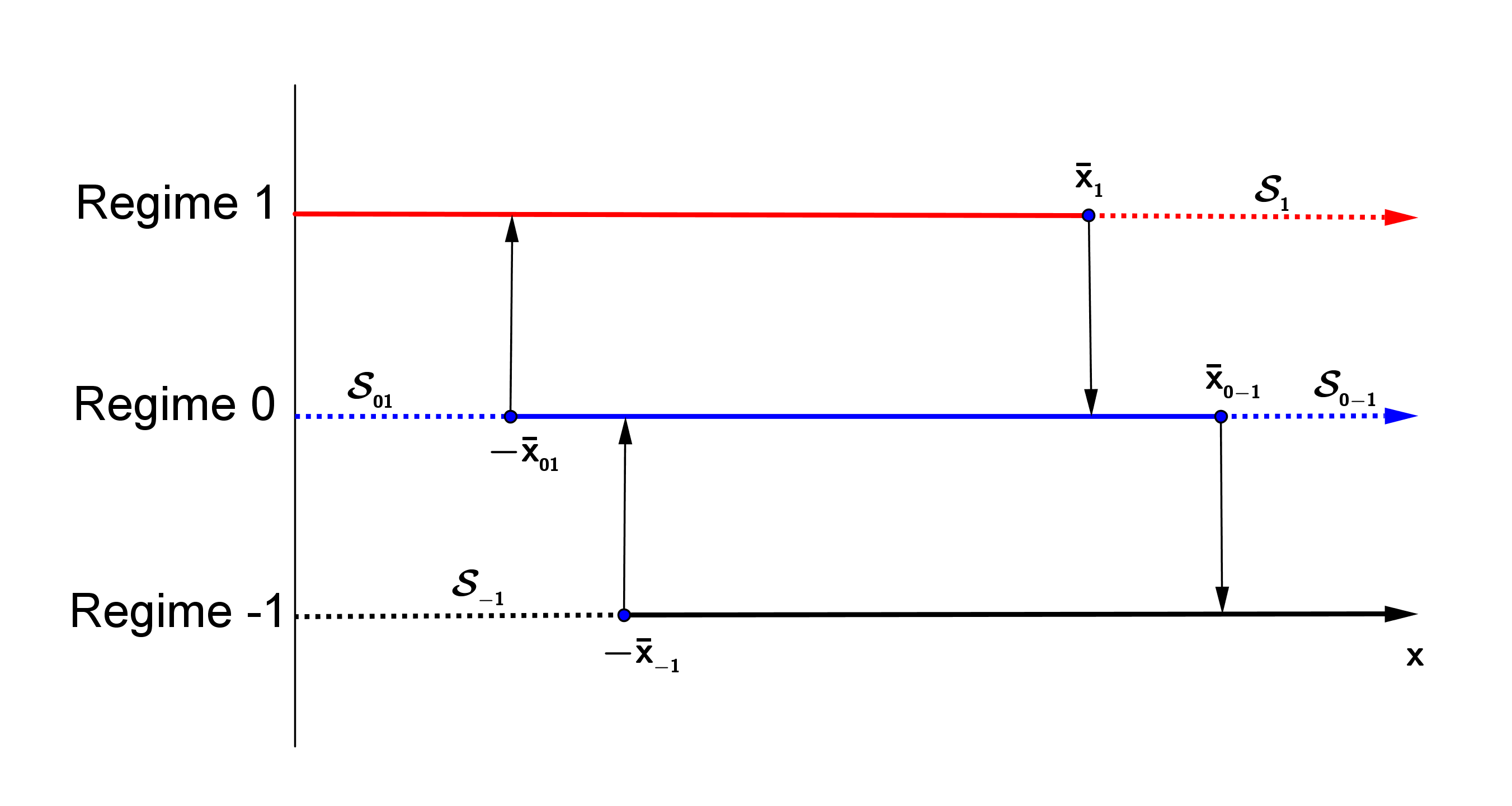
Figure 1: Regimes switching regions in cases (1) and (2)(i).

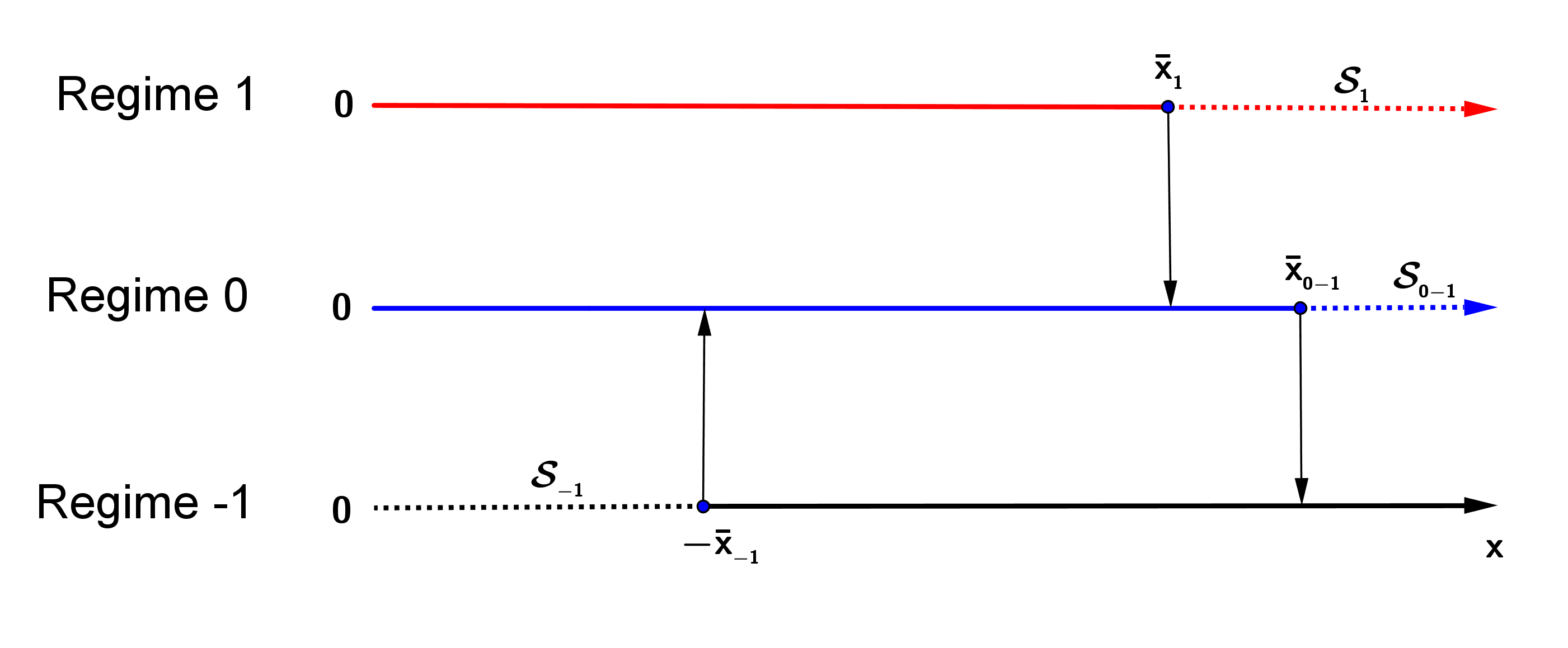
Figure 2: Regimes switching regions in case (2)(ii).

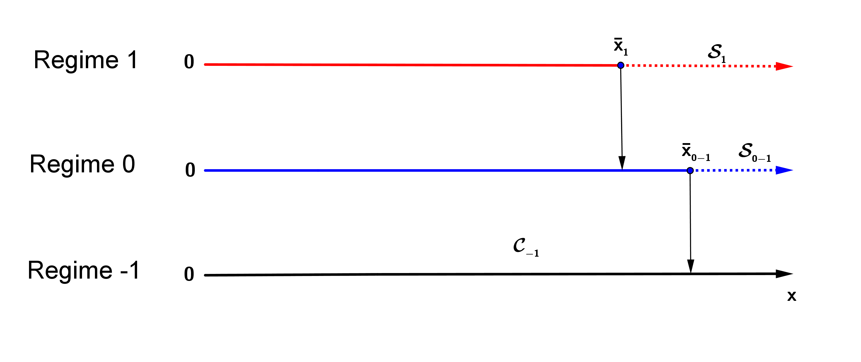
Figure 3: Regimes switching regions in case (2)(iii).

The next result provides the explicit solution to the optimal switching problem.

Theorem 4.1

$\bullet$ Case (1): $\ell_{-}$ $=$ $\infty$. The value functions are given by

$$v_{{}_{0}}(x) = \left\{\begin{array}[]{cc}A_{{}_{1}}\psi_{+}(x)-\frac{\lambda}{\rho}+g_{{}_{01}}(x),&x\leq-\bar{x}_{{}_{01}},\\ A_{{}_{0}}\psi_{+}(x)+B_{{}_{0}}\psi_{-}(x),&-\bar{x}_{{}_{01}}<x<\bar{x}_{{}_{0-1}},\\ B_{{}_{-1}}\psi_{-}(x)-\frac{\lambda}{\rho}+g_{{}_{0-1}}(x),&x\geq\bar{x}_{{}_{0-1}},\end{array}\right.$$

$$v_{{}_{1}}(x) = \left\{\begin{array}[]{cc}A_{{}_{1}}\psi_{+}(x)-\frac{\lambda}{\rho},&x<\bar{x}_{{}_{1}},\\ v_{{}_{0}}(x)+g_{{}_{10}}(x),&x\geq\bar{x}_{{}_{1}},\end{array}\right.$$

$$v_{{}_{-1}}(x) = \left\{\begin{array}[]{cc}v_{{}_{0}}(x)+g_{{}_{-10}}(x),&x\leq-\bar{x}_{{}_{-1}},\\ B_{{}_{-1}}\psi_{-}(x)-\frac{\lambda}{\rho},&x>-\bar{x}_{{}_{-1}},\end{array}\right.$$

and the constants $A_{{}_{0}}$, $B_{{}_{0}}$, $A_{{}_{1}}$, $B_{{}_{-1}}$, $\bar{x}_{{}_{01}}$, $\bar{x}_{{}_{0-1}}$, $\bar{x}_{{}_{1}}$, $\bar{x}_{{}_{-1}}$ are determined by the smooth-fit conditions:

$$A_{{}_{1}}\psi_{+}(-\bar{x}_{{}_{01}})-\frac{\lambda}{\rho}+g_{{}_{01}}(-\bar{x}_{{}_{01}}) = A_{{}_{0}}\psi_{+}(-\bar{x}_{{}_{01}})+B_{{}_{0}}\psi_{-}(-\bar{x}_{{}_{01}})$$

$$A_{{}_{1}}\psi_{+}^{\prime}(-\bar{x}_{{}_{01}})-1 = A_{{}_{0}}\psi_{+}^{\prime}(-\bar{x}_{{}_{01}})+B_{{}_{0}}\psi_{-}^{\prime}(-\bar{x}_{{}_{01}})$$

$$B_{{}_{-1}}\psi_{-}(\bar{x}_{{}_{0-1}})-\frac{\lambda}{\rho}+g_{{}_{0-1}}(\bar{x}_{{}_{0-1}}) = A_{{}_{0}}\psi_{+}(\bar{x}_{{}_{0-1}})+B_{{}_{0}}\psi_{-}(\bar{x}_{{}_{0-1}})$$

$$B_{{}_{-1}}\psi_{-}^{\prime}(\bar{x}_{{}_{0-1}})+1 = A_{{}_{0}}\psi_{+}^{\prime}(\bar{x}_{{}_{0-1}})+B_{{}_{0}}\psi_{-}^{\prime}(\bar{x}_{{}_{0-1}})$$

$$A_{{}_{1}}\psi_{+}(\bar{x}_{{}_{1}})-\frac{\lambda}{\rho} = A_{{}_{0}}\psi_{+}(\bar{x}_{{}_{1}})+B_{{}_{0}}\psi_{-}(\bar{x}_{{}_{1}})+g_{{}_{10}}(\bar{x}_{{}_{1}})$$

$$A_{{}_{1}}\psi_{+}^{\prime}(\bar{x}_{{}_{1}}) = A_{{}_{0}}\psi_{+}^{\prime}(\bar{x}_{{}_{1}})+B_{{}_{0}}\psi_{-}^{\prime}(\bar{x}_{{}_{1}})+1$$

$$B_{{}_{-1}}\psi_{-}(-\bar{x}_{{}_{-1}})-\frac{\lambda}{\rho} = A_{{}_{0}}\psi_{+}(-\bar{x}_{{}_{-1}})+B_{{}_{0}}\psi_{-}(-\bar{x}_{{}_{-1}})+g_{{}_{-10}}(-\bar{x}_{{}_{-1}})$$

$$B_{{}_{-1}}\psi_{-}^{\prime}(-\bar{x}_{{}_{-1}}) = A_{{}_{0}}\psi_{+}^{\prime}(-\bar{x}_{{}_{-1}})+B_{{}_{0}}\psi_{-}^{\prime}(-\bar{x}_{{}_{-1}})-1.$$

$\bullet$ Case (2)(i): $\ell_{-}$ $=$ $0$, and both ${\cal S}_{{}_{-1}}$ and ${\cal S}_{{}_{01}}$ are not empty. The value functions have the same form as Case (1) with the state space domain $(0,\infty)$.

$\bullet$ Case (2)(ii): $\ell_{-}$ $=$ $0$, ${\cal S}_{{}_{-1}}$ is not empty, and ${\cal S}_{{}_{01}}$ $=$ $\emptyset$. The value functions are given by

$$v_{{}_{0}}(x) = \left\{\begin{array}[]{cc}A_{{}_{0}}\psi_{+}(x),&0<x<\bar{x}_{{}_{0-1}},\\ B_{{}_{-1}}\psi_{-}(x)-\frac{\lambda}{\rho}+g_{{}_{0-1}}(x),&x\geq\bar{x}_{{}_{0-1}},\end{array}\right.$$

$$v_{{}_{-1}}(x) = \left\{\begin{array}[]{cc}v_{{}_{0}}(x)+g_{{}_{-10}}(x),&0<x\leq-\bar{x}_{{}_{-1}},\\ B_{{}_{-1}}\psi_{-}(x)-\frac{\lambda}{\rho},&x>-\bar{x}_{{}_{-1}},\end{array}\right.$$

$$v_{{}_{1}}(x) = \left\{\begin{array}[]{cc}A_{{}_{1}}\psi_{+}(x)-\frac{\lambda}{\rho},&0<x<\max(\bar{x}_{{}_{1}},0),\\ v_{{}_{0}}(x)+g_{{}_{10}}(x),&x\geq\max(\bar{x}_{{}_{1}},0),\end{array}\right.$$

and the constants $A_{{}_{0}}$, $A_{{}_{1}}$, $B_{{}_{-1}}$, $\bar{x}_{{}_{0-1}}$ $>$ $0$, $\bar{x}_{{}_{1}}$, $\bar{x}_{{}_{-1}}$ $<$ $0$ are determined by the smooth-fit conditions:

$$B_{{}_{-1}}\psi_{-}(\bar{x}_{{}_{0-1}})-\frac{\lambda}{\rho}+g_{{}_{0-1}}(\bar{x}_{{}_{0-1}}) = A_{{}_{0}}\psi_{+}(\bar{x}_{{}_{0-1}})$$

$$B_{{}_{-1}}\psi_{-}^{\prime}(\bar{x}_{{}_{0-1}})+1 = A_{{}_{0}}\psi_{+}^{\prime}(\bar{x}_{{}_{0-1}})$$

$$A_{{}_{1}}\psi_{+}(\bar{x}_{{}_{1}})-\frac{\lambda}{\rho} = A_{{}_{0}}\psi_{+}(\bar{x}_{{}_{1}})+g_{{}_{10}}(\bar{x}_{{}_{1}})$$

$$A_{{}_{1}}\psi_{+}^{\prime}(\bar{x}_{{}_{1}}) = A_{{}_{0}}\psi_{+}^{\prime}(\bar{x}_{{}_{1}})+1$$

$$B_{{}_{-1}}\psi_{-}(-\bar{x}_{{}_{-1}})-\frac{\lambda}{\rho} = A_{{}_{0}}\psi_{+}(-\bar{x}_{{}_{-1}})+g_{{}_{-10}}(-\bar{x}_{{}_{-1}})$$

$$B_{{}_{-1}}\psi_{-}^{\prime}(-\bar{x}_{{}_{-1}}) = A_{{}_{0}}\psi_{+}^{\prime}(-\bar{x}_{{}_{-1}})-1.$$

$\bullet$ Case (2)(iii): $\ell_{-}$ $=$ $0$, and ${\cal S}_{{}_{-1}}$ $=$ ${\cal S}_{{}_{01}}$ $=$ $\emptyset$. The value functions are given by

$$v_{{}_{0}}(x) = \left\{\begin{array}[]{cc}A_{{}_{0}}\psi_{+}(x),&0<x<\bar{x}_{{}_{0-1}},\\ -\frac{\lambda}{\rho}+g_{{}_{0-1}}(x),&x\geq\bar{x}_{{}_{0-1}},\end{array}\right.$$

$$v_{{}_{1}}(x) = \left\{\begin{array}[]{cc}A_{{}_{1}}\psi_{+}(x)-\frac{\lambda}{\rho},&x<\bar{x}_{{}_{1}},\\ v_{{}_{0}}(x)+g_{{}_{10}}(x),&x\geq\bar{x}_{{}_{1}},\end{array}\right.$$

$$v_{{}_{-1}}=-\frac{\lambda}{\rho},$$

and the constants $A_{{}_{0}}$, $A_{{}_{1}}$, $\bar{x}_{{}_{0-1}}$ $>$ $0$, $\bar{x}_{{}_{1}}$ $>$ $0$, are determined by the smooth-fit conditions:

$$-\frac{\lambda}{\rho}+g_{{}_{0-1}}(\bar{x}_{{}_{0-1}}) = A_{{}_{0}}\psi_{+}(\bar{x}_{{}_{0-1}})$$

$$1 = A_{{}_{0}}\psi_{+}^{\prime}(\bar{x}_{{}_{0-1}})$$

$$A_{{}_{1}}\psi_{+}(\bar{x}_{{}_{1}})-\frac{\lambda}{\rho} = A_{{}_{0}}\psi_{+}(\bar{x}_{{}_{1}})+g_{{}_{10}}(\bar{x}_{{}_{1}})$$

$$A_{{}_{1}}\psi_{+}^{\prime}(\bar{x}_{{}_{1}}) = A_{{}_{0}}\psi_{+}^{\prime}(\bar{x}_{{}_{1}})+1.$$

Proof. We consider only case (1) and (2)(i) since the other cases are dealt with by similar arguments. We have ${\cal S}_{{}_{01}}\;=\;(\ell_{-},-\bar{x}_{{}_{01}}]$, which means that $v_{{}_{0}}=v_{{}_{1}}+g_{{}_{01}}$ on $(\ell_{-},-\bar{x}_{{}_{01}}]$. Moreover, $v_{{}_{1}}$ is solution to $\rho v_{{}_{1}}-{\cal L}v_{{}_{1}}+\lambda=0$ on $(\ell_{-},\bar{x}_{{}_{1}})$, which combined with the bound in the Lemma 3.1, shows that $v_{{}_{1}}$ should be in the form: $v_{{}_{1}}$ $=$ $A_{{}_{1}}\psi_{+}-\frac{\lambda}{\rho}$ on $(\ell_{-},\bar{x}_{{}_{1}})$. Since $-\bar{x}_{{}_{01}}<\bar{x}_{{}_{1}}$, we deduce that $v_{{}_{0}}$ has the form expressed as: $A_{{}_{1}}\psi_{+}-\frac{\lambda}{\rho}+g_{{}_{01}}$ on $(\ell_{-},-\bar{x}_{{}_{01}}]$. In the same way, $v_{{}_{-1}}$ should have the form expressed as $B_{{}_{-1}}\psi_{-}-\frac{\lambda}{\rho}$ on $(-\bar{x}_{{}_{-1}},\infty)$ and $v_{{}_{0}}$ has the form expressed as $B_{{}_{-1}}\psi_{-}-\frac{\lambda}{\rho}+g_{{}_{0-1}}$ on $[\bar{x}_{{}_{0-1}},\infty)$. We know that $v_{{}_{0}}$ is solution to $\rho v_{{}_{0}}-{\cal L}v_{{}_{0}}=0$ on $(-\bar{x}_{{}_{01}},\bar{x}_{{}_{0-1}})$ so that $v_{{}_{0}}$ should be in the form: $v_{{}_{0}}$ $=$ $A_{{}_{0}}\psi_{+}+B_{{}_{0}}\psi_{-}$ on $(-\bar{x}_{{}_{01}},\bar{x}_{{}_{0-1}})$. We have ${\cal S}_{{}_{1}}\;=\;[\bar{x}_{{}_{1}},\infty)$, which means that $v_{{}_{1}}$ $=$ $v_{{}_{0}}+g_{{}_{10}}$ on $[\bar{x}_{{}_{1}},\infty)$ and ${\cal S}_{{}_{-1}}\;=\;(\ell_{-},-\bar{x}_{{}_{-1}}]$, which means that $v_{{}_{-1}}=v_{{}_{0}}+g_{{}_{-10}}$ on $(\ell_{-},-\bar{x}_{{}_{-1}}]$. From Proposition 4.1 we know that $\bar{x}_{{}_{1}}$ $\leq$ $\bar{x}_{{}_{0-1}}$, and $-\bar{x}_{{}_{01}}$ $\leq$ $-\bar{x}_{{}_{-1}}$ and by the smooth-fit property of value function we obtain the above smooth-fit condition equations in which we can compute the cut-off points by solving these quasi-algebraic equations. $\Box$

Remark 4.4

1. In Case (1) and Case(2)(i) of Theorem 4.1, the smooth-fit conditions system is written as:

$$\left[\begin{array}[]{cccc}\psi_{+}(-\bar{x}_{{}_{01}})&0&-\psi_{+}(-\bar{x}_{{}_{01}})&-\psi_{-}(-\bar{x}_{{}_{01}})\\ 0&\psi_{-}(\bar{x}_{{}_{0-1}})&-\psi_{+}(\bar{x}_{{}_{0-1}})&-\psi_{-}(\bar{x}_{{}_{0-1}})\\ \psi_{+}(\bar{x}_{{}_{1}})&0&-\psi_{+}(\bar{x}_{{}_{1}})&-\psi_{-}(\bar{x}_{{}_{1}})\\ 0&\psi_{-}(-\bar{x}_{{}_{-1}})&-\psi_{+}(-\bar{x}_{{}_{-1}})&-\psi_{-}(-\bar{x}_{{}_{-1}})\end{array}\right]\times\left[\begin{array}[]{c}A_{{}_{1}}\\ B_{{}_{-1}}\\ A_{{}_{0}}\\ B_{{}_{0}}\end{array}\right]=\left[\begin{array}[]{c}\lambda\rho^{-1}-g_{{}_{01}}(-\bar{x}_{{}_{01}})\\ \lambda\rho^{-1}-g_{{}_{0-1}}(\bar{x}_{{}_{0-1}})\\ \lambda\rho^{-1}+g_{{}_{10}}(\bar{x}_{{}_{1}})\\ \lambda\rho^{-1}+g_{{}_{-10}}(-\bar{x}_{{}_{-1}})\end{array}\right]$$ (4.28)

and

$$\left[\begin{array}[]{cccc}\psi_{+}^{{}^{\prime}}(-\bar{x}_{{}_{01}})&0&-\psi_{+}^{{}^{\prime}}(-\bar{x}_{{}_{01}})&-\psi_{-}^{{}^{\prime}}(-\bar{x}_{{}_{01}})\\ 0&\psi_{-}^{{}^{\prime}}(\bar{x}_{{}_{0-1}})&-\psi_{+}^{{}^{\prime}}(\bar{x}_{{}_{0-1}})&-\psi_{-}^{{}^{\prime}}(\bar{x}_{{}_{0-1}})\\ \psi_{+}^{{}^{\prime}}(\bar{x}_{{}_{1}})&0&-\psi_{+}^{{}^{\prime}}(\bar{x}_{{}_{1}})&-\psi_{-}^{{}^{\prime}}(\bar{x}_{{}_{1}})\\ 0&\psi_{-}^{{}^{\prime}}(-\bar{x}_{{}_{-1}})&-\psi_{+}^{{}^{\prime}}(-\bar{x}_{{}_{-1}})&-\psi_{-}^{{}^{\prime}}(-\bar{x}_{{}_{-1}})\end{array}\right]\times\left[\begin{array}[]{c}A_{{}_{1}}\\ B_{{}_{-1}}\\ A_{{}_{0}}\\ B_{{}_{0}}\end{array}\right]=\left[\begin{array}[]{c}1\\ -1\\ 1\\ -1\end{array}\right].$$ (4.42)

Denote by $M(\bar{x}_{{}_{01}},\bar{x}_{{}_{0-1}},\bar{x}_{{}_{1}},\bar{x}_{{}_{-1}})$ and $M_{x}(\bar{x}_{{}_{01}},\bar{x}_{{}_{0-1}},\bar{x}_{{}_{1}},\bar{x}_{{}_{-1}})$ the matrices:

$$M(\bar{x}_{{}_{01}},\bar{x}_{{}_{0-1}},\bar{x}_{{}_{1}},\bar{x}_{{}_{-1}}) = \left[\begin{array}[]{cccc}\psi_{+}(-\bar{x}_{{}_{01}})&0&0&-\psi_{-}(-\bar{x}_{{}_{01}})\\ 0&\psi_{-}(\bar{x}_{{}_{0-1}})&-\psi_{+}(\bar{x}_{{}_{0-1}})&0\\ \psi_{+}(\bar{x}_{{}_{1}})&0&0&-\psi_{-}(\bar{x}_{{}_{1}})\\ 0&\psi_{-}(-\bar{x}_{{}_{-1}})&-\psi_{+}(-\bar{x}_{{}_{-1}})&0\end{array}\right],$$

$$M_{x}(\bar{x}_{{}_{01}},\bar{x}_{{}_{0-1}},\bar{x}_{{}_{1}},\bar{x}_{{}_{-1}}) = \left[\begin{array}[]{cccc}\psi_{+}^{{}^{\prime}}(-\bar{x}_{{}_{01}})&0&0&-\psi_{-}^{{}^{\prime}}(-\bar{x}_{{}_{01}})\\ 0&\psi_{-}^{{}^{\prime}}(\bar{x}_{{}_{0-1}})&-\psi_{+}^{{}^{\prime}}(\bar{x}_{{}_{0-1}})&0\\ \psi_{+}^{{}^{\prime}}(\bar{x}_{{}_{1}})&0&0&-\psi_{-}^{{}^{\prime}}(\bar{x}_{{}_{1}})\\ 0&\psi_{-}^{{}^{\prime}}(-\bar{x}_{{}_{-1}})&-\psi_{+}^{{}^{\prime}}(-\bar{x}_{{}_{-1}})&0\end{array}\right].$$

Once $M(\bar{x}_{{}_{01}},\bar{x}_{{}_{0-1}},\bar{x}_{{}_{1}},\bar{x}_{{}_{-1}})$ and $M_{x}(\bar{x}_{{}_{01}},\bar{x}_{{}_{0-1}},\bar{x}_{{}_{1}},\bar{x}_{{}_{-1}})$ are nonsingular, straightforward computations from (4.28) and (4.42) lead to the following equation satisfied by $\bar{x}_{{}_{01}}$, $\bar{x}_{{}_{0-1}}$, $\bar{x}_{{}_{1}}$, $\bar{x}_{{}_{-1}}$:

$$M_{x}(\bar{x}_{{}_{01}},\bar{x}_{{}_{0-1}},\bar{x}_{{}_{1}},\bar{x}_{{}_{-1}})^{-1}\left[\begin{array}[]{c}1\\ -1\\ 1\\ -1\end{array}\right] = M(\bar{x}_{{}_{01}},\bar{x}_{{}_{0-1}},\bar{x}_{{}_{1}},\bar{x}_{{}_{-1}})^{-1}\left[\begin{array}[]{c}\lambda\rho^{-1}-g_{{}_{01}}(-\bar{x}_{{}_{01}})\\ \lambda\rho^{-1}-g_{{}_{0-1}}(\bar{x}_{{}_{0-1}})\\ \lambda\rho^{-1}+g_{{}_{10}}(\bar{x}_{{}_{1}})\\ \lambda\rho^{-1}+g_{{}_{-10}}(-\bar{x}_{{}_{-1}})\end{array}\right].$$

This system can be separated into two independent systems:

$$\left[\begin{array}[]{cccc}\psi_{+}^{{}^{\prime}}(-\bar{x}_{{}_{01}})&-\psi_{-}^{{}^{\prime}}(-\bar{x}_{{}_{01}})\\ \psi_{+}^{{}^{\prime}}(\bar{x}_{{}_{1}})&-\psi_{-}^{{}^{\prime}}(\bar{x}_{{}_{1}})\\ \end{array}\right]^{-1}\times\left[\begin{array}[]{c}1\\ 1\end{array}\right]=$$ (4.50)

$$\left[\begin{array}[]{cccc}\psi_{+}(-\bar{x}_{{}_{01}})&-\psi_{-}(-\bar{x}_{{}_{01}})\\ \psi_{+}(\bar{x}_{{}_{1}})&-\psi_{-}(\bar{x}_{{}_{1}})\\ \end{array}\right]^{-1}\times\left[\begin{array}[]{c}\lambda\rho^{-1}-g_{{}_{01}}(-\bar{x}_{{}_{01}})\\ \lambda\rho^{-1}+g_{{}_{10}}(\bar{x}_{{}_{1}})\\ \end{array}\right]$$ (4.55)

and

$$\left[\begin{array}[]{cccc}\psi_{-}^{{}^{\prime}}(\bar{x}_{{}_{0-1}})&-\psi_{+}^{{}^{\prime}}(\bar{x}_{{}_{0-1}})\\ \psi_{-}^{{}^{\prime}}(-\bar{x}_{{}_{-1}})&-\psi_{+}^{{}^{\prime}}(-\bar{x}_{{}_{-1}})\end{array}\right]^{-1}\times\left[\begin{array}[]{c}-1\\ -1\end{array}\right]=$$ (4.60)

$$\left[\begin{array}[]{cccc}\psi_{-}(\bar{x}_{{}_{0-1}})&-\psi_{+}(\bar{x}_{{}_{0-1}})\\ \psi_{-}(-\bar{x}_{{}_{-1}})&-\psi_{+}(-\bar{x}_{{}_{-1}})\end{array}\right]^{-1}\times\left[\begin{array}[]{c}\lambda\rho^{-1}-g_{{}_{0-1}}(\bar{x}_{{}_{0-1}})\\ \lambda\rho^{-1}+g_{{}_{-10}}(-\bar{x}_{{}_{-1}})\end{array}\right]$$ (4.65)

We then obtain thresholds $\bar{x}_{{}_{01}}$, $\bar{x}_{{}_{0-1}}$, $\bar{x}_{{}_{1}}$, $\bar{x}_{{}_{-1}}$ by solving two quasi-algebraic system equations (4.50) and (4.60). Notice that for the examples of OU or IGBM process, the matrices $M(\bar{x}_{{}_{01}},\bar{x}_{{}_{0-1}},\bar{x}_{{}_{1}},\bar{x}_{{}_{-1}})$ and $M_{x}(\bar{x}_{{}_{01}},\bar{x}_{{}_{0-1}},\bar{x}_{{}_{1}},\bar{x}_{{}_{-1}})$ are nonsingular so that their inverses are well-defined. Indeed, we have: $\psi_{+}^{{}^{\prime\prime}}$ $>$ $0$ and $\psi_{-}^{{}^{\prime\prime}}$ $>$ $0$. This property is trivial for the case of OU process, while for the case of IGBM:

$$\frac{d^{2}\psi_{+}(x)}{dx^{2}} = \frac{d}{dx}\left(\frac{a}{x^{a+1}}(-U(a+1,b,\frac{c}{x})(a-b+1))\right)$$

$$= \frac{a(a+1)}{x^{a+2}}U(a+2,b,\frac{c}{x})(a-b+1)(a-b+2)>0,\ \ \forall x>0.$$

$$\frac{d\psi_{-}(x)}{dx} = -\frac{ax^{-a-2}(bxM(a,b,\frac{c}{x})+cM(a+1,b+1,\frac{c}{x}))}{b},\ \ \forall x>0.$$

Thus, $\psi_{-}^{{}^{\prime}}$ is strictly increasing since $M(a,b,\frac{c}{x})$ is strictly decreasing, and so $\psi_{-}^{{}^{\prime\prime}}$ $>$ $0$. Moreover, we have:

$$\text{det}\;\big{[}M(\bar{x}_{{}_{01}},\bar{x}_{{}_{0-1}},\bar{x}_{{}_{1}},\bar{x}_{{}_{-1}})\big{]}$$

$$= \left(\psi_{-}(\bar{x}_{{}_{-01}})\psi_{+}(\bar{x}_{{}_{1}})-\psi_{-}(\bar{x}_{{}_{1}})\psi_{+}(\bar{x}_{{}_{-01}})\right)\left(\psi_{-}(\bar{x}_{{}_{0-1}})\psi_{+}(\bar{x}_{{}_{-1}})-\psi_{-}(\bar{x}_{{}_{-1}})\psi_{+}(\bar{x}_{{}_{0-1}})\right).$$

Recalling that $-\bar{x}_{{}_{01}}$ $<$ $\bar{x}_{{}_{1}}$ and $\bar{x}_{{}_{0-1}}$ $>$ $-\bar{x}_{{}_{-1}}$ (see Proposition 4.1), and since $\psi_{+}$ is a strictly increasing and positive function, while $\psi_{-}$ is a strictly decreasing positive function, we have: $\psi_{-}(\bar{x}_{{}_{-01}})\psi_{+}(\bar{x}_{{}_{1}})-\psi_{-}(\bar{x}_{{}_{1}})\psi_{+}(\bar{x}_{{}_{-01}})$ $>$ $0$ and $\psi_{-}(\bar{x}_{{}_{0-1}})\psi_{+}(\bar{x}_{{}_{-1}})-\psi_{-}(\bar{x}_{{}_{-1}})\psi_{+}(\bar{x}_{{}_{0-1}})$ $<$ $0$, which implies the non singularity of the matrix $M(\bar{x}_{{}_{01}},\bar{x}_{{}_{0-1}},\bar{x}_{{}_{1}},\bar{x}_{{}_{-1}})$. On the other hand, we have:

$$\text{det}\big{[}M_{x}(\bar{x}_{{}_{01}},\bar{x}_{{}_{0-1}},\bar{x}_{{}_{1}},\bar{x}_{{}_{-1}})\big{]}$$

$$= \left(\psi_{-}^{{}^{\prime}}(\bar{x}_{{}_{-01}})\psi_{+}^{{}^{\prime}}(\bar{x}_{{}_{1}})-\psi_{-}^{{}^{\prime}}(\bar{x}_{{}_{1}})\psi_{+}^{{}^{\prime}}(\bar{x}_{{}_{-01}})\right)\left(\psi_{-}^{{}^{\prime}}(\bar{x}_{{}_{0-1}})\psi_{+}^{{}^{\prime}}(\bar{x}_{{}_{-1}})-\psi_{-}^{{}^{\prime}}(\bar{x}_{{}_{-1}})\psi_{+}^{{}^{\prime}}(\bar{x}_{{}_{0-1}})\right).$$

Since $\psi_{+}^{\prime}$ is a strictly increasing positive function and $\psi_{-}^{\prime}$ is a strictly increasing function, with $\psi_{-}^{\prime}$ $<$ $0$, we get: $\psi_{-}^{{}^{\prime}}(\bar{x}_{{}_{-01}})\psi_{+}^{{}^{\prime}}(\bar{x}_{{}_{1}})-\psi_{-}^{{}^{\prime}}(\bar{x}_{{}_{1}})\psi_{+}^{{}^{\prime}}(\bar{x}_{{}_{-01}})$ $<$ $0$ and $\psi_{-}^{{}^{\prime}}(\bar{x}_{{}_{0-1}})\psi_{+}^{{}^{\prime}}(\bar{x}_{{}_{-1}})-\psi_{-}^{{}^{\prime}}(\bar{x}_{{}_{-1}})\psi_{+}^{{}^{\prime}}(\bar{x}_{{}_{0-1}})$ $>$ $0$, which implies the non singularity of the matrix $M_{x}(\bar{x}_{{}_{01}},\bar{x}_{{}_{0-1}},\bar{x}_{{}_{1}},\bar{x}_{{}_{-1}})$.

2. In Case (2)(ii) of Theorem 4.1, we obtain the thresholds $\bar{x}_{{}_{0-1}}$ $>$ $0$, $\bar{x}_{{}_{-1}}$ $<$ $0$ from the smooth-fit conditions which lead to the quasi-algebraic system:

$$\left[\begin{array}[]{cccc}-\psi_{-}^{{}^{\prime}}(\bar{x}_{{}_{0-1}})&\psi_{+}^{{}^{\prime}}(\bar{x}_{{}_{0-1}})\\ -\psi_{-}^{{}^{\prime}}(-\bar{x}_{{}_{-1}})&\psi_{+}^{{}^{\prime}}(-\bar{x}_{{}_{-1}})\end{array}\right]^{-1}\times\left[\begin{array}[]{c}1\\ 1\end{array}\right]=$$ (4.72)

$$\left[\begin{array}[]{cccc}-\psi_{-}(\bar{x}_{{}_{0-1}})&\psi_{+}(\bar{x}_{{}_{0-1}})\\ -\psi_{-}(-\bar{x}_{{}_{-1}})&\psi_{+}(-\bar{x}_{{}_{-1}})\end{array}\right]^{-1}\times\left[\begin{array}[]{c}-\lambda\rho^{-1}+g_{{}_{0-1}}(\bar{x}_{{}_{0-1}})\\ -\lambda\rho^{-1}-g_{{}_{-10}}(-\bar{x}_{{}_{-1}})\end{array}\right].$$ (4.77)

The non singularity of the matrix above is checked similarly as in case (1) and (2)(i) for the examples of the OU or IGBM process. Note that $\bar{x}_{{}_{0-1}}$, $\bar{x}_{{}_{-1}}$ are independent from $\bar{x}_{{}_{1}}$, which is obtained from the equation:

$$\left(-\lambda\rho^{-1}-g_{{}_{10}}(\bar{x}_{{}_{1}})\right)\psi_{+}^{{}^{\prime}}(\bar{x}_{{}_{1}})+\psi_{+}(\bar{x}_{{}_{1}})=0.$$ (4.78)

When $\bar{x}_{{}_{1}}$ $\leq$ $0$, this means that ${\cal S}_{{}_{1}}$ $=$ $(0,\infty)$.

3. In Case (2)(iii) of Theorem 4.1, the threshold $\bar{x}_{{}_{1}}$ $>$ $0$ is obtained from the equation (4.78), while the threshold $\bar{x}_{{}_{0-1}}$ $>$ $0$ is derived from the smooth-fit condition leading to the quasi-algebraic equation:

$$\left(\lambda\rho^{-1}-g_{{}_{0-1}}(\bar{x}_{{}_{0-1}})\right)\psi_{+}^{{}^{\prime}}(\bar{x}_{{}_{0-1}})+\psi_{+}(\bar{x}_{{}_{0-1}})=0.$$ (4.79)

$\Box$

5 Numerical examples

In this part, we consider OU process and IGBM as examples.

• We first consider the example of the Ornstein-Uhlenbeck process:

$$dX_{t} = -\mu X_{t}dt+\sigma dW_{t},$$

with $\mu$, $\sigma$ positive constants. In this case, the two fundamental solutions to (3.1) are given by

$$\psi_{+}(x)=\int_{0}^{\infty}t^{\frac{\rho}{\mu}-1}\exp\big{(}-\frac{t^{2}}{2}+\frac{\sqrt{2\mu}}{\sigma}xt\big{)}dt, \psi_{-}(x)=\int_{0}^{\infty}t^{\frac{\rho}{\mu}-1}\exp\big{(}-\frac{t^{2}}{2}-\frac{\sqrt{2\mu}}{\sigma}xt\big{)}dt,$$

and satisfy assumption (3.3). We consider a numerical example with the following specifications: : $\mu=0.8$ , $\sigma=0.5$ , $\rho=0.1$ , $\lambda=0.07$ , $\varepsilon=0.005$ , $L=0$.

Remark 5.1

We can reduce the case of non zero long run mean $L\neq 0$ of the OU process to the case of $L=0$ by considering process $Y_{t}=X_{t}-L$ as spread process, because in this case $\sigma$ is constant. Finally, we can see that, cutoff points translate along $L$, as illustrated in figure 6. $\Box$

We recall some notations:
${\cal S}_{{}_{01}}\;=\;(-\infty,-\bar{x}_{{}_{01}}]$ is the open-to-buy region,
${\cal S}_{{}_{0-1}}\;=\;[\bar{x}_{{}_{0-1}},\infty)$ is the open-to-sell region,
${\cal S}_{{}_{1}}\;=\;[\bar{x}_{{}_{1}},\infty)$ is Sell-to-close region from the long position $i$ $=$ $1$,
${\cal S}_{{}_{-1}}\;=\;(-\infty,-\bar{x}_{{}_{-1}}]$ is Buy-to-close region from the short position $i$ $=$ $-1$.

We solve the two systems (4.50) and (4.60) which give

$$\bar{x}_{{}_{01}}=0.2094,\;\bar{x}_{{}_{1}}=0.0483,\;\bar{x}_{{}_{-1}}=0.0483,\;\bar{x}_{{}_{0-1}}=0.2094,$$

and confirm the symmetry property in Proposition 4.2.

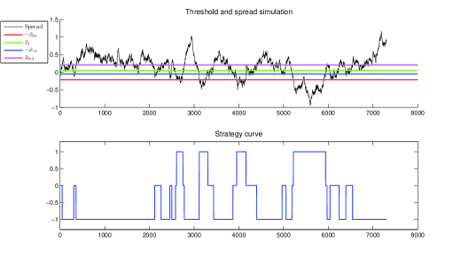
Figure 4: Simulation of trading strategies

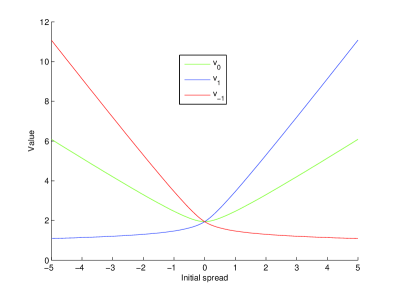
Figure 5: Value functions

In figure 5, we see the symmetry property of value functions as showed in Proposition 4.2. Moreover, we can see that $v_{{}_{1}}$ is a non decreasing function while $v_{{}_{-1}}$ is non increasing.

The next figure shows the dependence of cut-off point on parameters

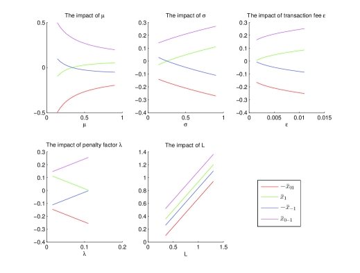
Figure 6: The dependence of cut-off point on parameters

In figure 6, $\mu$ measures the speed of mean reversion and we see that the length of intervals ${\cal S}_{{}_{01}}$, ${\cal S}_{{}_{0-1}}$ increases and the length of intervals ${\cal S}_{{}_{1}}$, ${\cal S}_{{}_{-1}}$ decreases as $\mu$ gets bigger. The length of intervals ${\cal S}_{{}_{01}}$, ${\cal S}_{{}_{0-1}}$, ${\cal S}_{{}_{1}}$, and ${\cal S}_{{}_{-1}}$ decreases as volatility $\sigma$ gets bigger. $L$ is the long run mean , to which the process tends to revert, and we see that the cutoff points translate along $L$. We now look at the parameters that does not affect on the dynamic of spread: the length of intervals ${\cal S}_{{}_{01}}$, ${\cal S}_{{}_{0-1}}$, ${\cal S}_{{}_{1}}$, and ${\cal S}_{{}_{-1}}$ decreases as the transaction fee $\varepsilon$ gets bigger. Finally, the length of intervals ${\cal S}_{{}_{01}}$, ${\cal S}_{{}_{0-1}}$ decreases and the length of intervals ${\cal S}_{{}_{1}}$, ${\cal S}_{{}_{-1}}$ increases as the penalty factor $\lambda$ gets larger, which means that the holding time in flat position $i=0$ is longer and the opportunity to enter the flat position from the other position is bigger as the penalty factor $\lambda$ is increasing.

• We now consider the example of Inhomogeneous Geometric Brownian Motions which has stochastic volatility, see more details in Zhao [20] :

$$dX_{t}=\mu(L-X_{t})dt+\sigma X_{t}dW_{t},\;\;\;X_{{}_{0}}>0,$$

where $\mu$, $L$ and $\sigma$ are positive constants. Recall that in this case, the two fundamental solutions to (3.1) are given by

$$\psi_{+}(x)=x^{-a}U(a,b,\frac{c}{x}), \psi_{-}(x)=x^{-a}M(a,b,\frac{c}{x}),$$

where

$$a = \frac{\sqrt{\sigma^{4}+4(\mu+2\rho)\sigma^{2}+4\mu^{2}}-(2\mu+\sigma^{2})}{2\sigma^{2}}>0,$$

$$b = \frac{2\mu}{\sigma^{2}}+2a+2,\;\;\;\;\;c=\frac{2\mu L}{\sigma^{2}},$$

$M$ and $U$ are the confluent hypergeometric functions of the first and second kind. We can easily check that $\psi_{-}$ is a monotone decreasing function, while

$$\frac{d\psi_{+}(x)}{dx} = \frac{a}{x^{a+1}}(-U(a+1,b,\frac{c}{x})(a-b+1))>0,\ \ \forall x>0,$$

so that $\psi_{+}$ is a monotone increasing function. Moreover, by the asymptotic property of the confluent hypergeometric functions (cf.[1]), the fundamental solutions $\psi_{+}$ and $\psi_{-}$ satisfy the condition (3.3).

$\bullet$ Case (2)(i): Both ${\cal S}_{{}_{-1}}$ and ${\cal S}_{{}_{01}}$ are not empty. Let us consider a numerical example with the following specifications: : $\mu=0.8$ , $\sigma=0.5$ , $\rho=0.1$ , $\lambda=0.07$ , $\varepsilon=0.005$ , and we set $L=10$. Note that, in this case the condition in Lemma 4.3 is satisfied, and we solve the two systems (4.50) and (4.60) which give

$$\bar{x}_{{}_{01}}=-8.2777,\;\bar{x}_{{}_{1}}=9.3701,\;\bar{x}_{{}_{-1}}=-8.4283,\;\bar{x}_{{}_{0-1}}=9.5336.$$

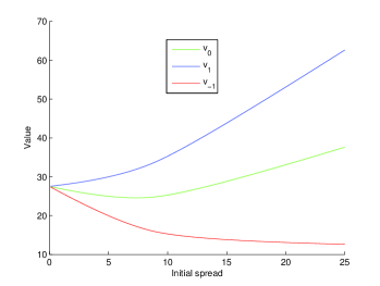
Figure 7: Value functions

In the figure 7, we can see that $v_{{}_{1}}$ is non decreasing while $v_{{}_{-1}}$ is non increasing. Moreover, $v_{{}_{1}}$ is always larger than $v_{{}_{0}}$, and $v_{{}_{-1}}$.

The next figure 8 shows the dependence of cut-off points on parameters (Note that the condition in Lemma 4.3 is satisfied for all parameters in this figure).

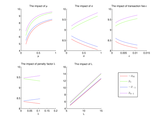
Figure 8: The dependence of cut-off point on parameters

We can make the same comments as in the case of the OU process, except for the dependence with respect to the long run mean $L$. Actually, we see that when $L$ increases, the moving of cutoff points is no more translational due to the non constant volatility.

$\bullet$ Case (2)(ii): ${\cal S}_{{}_{01}}$ is empty. Let us consider a numerical example with the following specifications: : $\mu=0.8$, $\sigma=0.3$, $\rho=0.1$, $\lambda=0.35$, $\varepsilon=0.55$, and $L=0.5$. We solve the two systems (4.72) and (4.78) which give

$$\bar{x}_{{}_{1}}=0.1187,\;\bar{x}_{{}_{-1}}=-0.8349,\;\bar{x}_{{}_{0-1}}=2.7504.$$

$\bullet$ Case (2)(iii): Both ${\cal S}_{{}_{-1}}$ and ${\cal S}_{{}_{01}}$ are empty. Let us consider a numerical example with the following specifications: : $\mu=0.8$, $\sigma=0.3$, $\rho=0.2$, $\lambda=0.05$, $\varepsilon=0.65$, and $L=0.1$. The two equations (4.79) and (4.78) give

$$\bar{x}_{{}_{1}}=0.4293,\;\bar{x}_{{}_{0-1}}=0.9560.$$

References

[1]
Abramowitz, M. and I. Stegun (1972): Handbook of mathematical functions: with formulas, graphs, and mathematical tables, Courier Dover Publications.
[2] Avellaneda, M. and J-H. Lee (2010): “Statistical arbitrage in the US equities market”, Quantitative Finance, 10, 761-782.
[3]
Bock, M. and R. Mestel (2009): “A regime-switching relative value arbitrage rule”, Operations Research Proceedings, 9-14, Springer.
[4]
Borodin, A. and P. Salminen (2002): Handbook of Brownian motion: facts and formulae, Springer.
[5]
Chen, Huafeng, Chen, Shaojun Jenny and F. Li (2012): “Empirical investigation of an equity pairs trading strategy”, preprint.
[6]
Do, B. and R. Faff (2010): “Does simple pairs trading still work?”, Financial Analysts Journal, 83-95.
[7]
Ehrman, D. (2006): The handbook of pairs trading: Strategies using equities, options, and futures, vol 240, John Wiley and Sons.
[8]
Ekstr m, E., Lindberg C. and J. Tysk (2011): “Optimal liquidation of a pairs trade”, Advanced mathematical methods for finance, Springer.
[9]
Elliott, R., Van der Hoek J. and W. Malcom (2005): “Pairs trading”, Quantitative Finance, vol 5, 271-276.
[10]
Kong, H. T. (2010): “Stochastic control and optimization of assets trading”, PhD thesis, University of Georgia.
[11]
Leung, T. and X. Li (2013): “Optimal Mean Reversion Trading with Transaction Costs and Stop-Loss Exit”, Social Science Research Network Working Paper Series.
[12]
Ly Vath, V. and H. Pham (2007): “Explicit solution to an optimal switching problem in the two-regime case”, SIAM Journal on Control and Optimization, vol 46, 395-426.
[13]
Mudchanatongsuk, S., Primbs J. and W. Wong (2008): “Optimal pairs trading: A stochastic control approach”, American Control Conference, IEEE, 2008.
[14]
Pham H. (2007): “On the smooth-fit property for one-dimensional optimal switching problem”, Séminaire de Probabilités XL, 187-199, Springer.
[15]
Pham, H., Ly Vath, V. and X.Y. Zhou (2009): “Optimal switching over multiple regimes”, SIAM Journal on Control and Optimization, vol 48, 2217-2253.
[17]
Tourin A. and R. Yan (2013): “Dynamic pairs trading using the stochastic control approach”, Journal of Economic Dynamics and Control, vol 37, 1972-1981.
[18]
Vidyamurthy, G. (2004): Pairs Trading: quantitative methods and analysis, John Wiley and Sons.
[19]
Zhang, H. and Q. Zhang (2008): “Trading a mean-reverting asset: Buy low and sell high”, Automatica, vol 44, 1511-1518.
[20]
Zhao B. (2009): “Inhomogeneous geometric Brownian motions”, Available at SSRN 1429449.