Homoclinic orbit and hidden attractor in the Lorenz-like system
describing the fluid convection motion in the rotating cavity
Abstract
In this paper a Lorenz-like system, describing the process of rotating fluid convection, is considered. The present work demonstrates numerically that this system, also like the classical Lorenz system, possesses a homoclinic trajectory and a chaotic self-excited attractor. However, for considered system, unlike the classical Lorenz one, along with self-excited attractor a hidden attractor can be localized. Analytical-numerical localization of hidden attractor is presented.
I Introduction
Consider the following physical problem: the convection of viscous incompressible fluid flow inside the ellipsoid
under the condition of stationary inhomogeneous external heating. It is assumed that the ellipsoid together with heat sources rotates with the constant velocity around its axis. The axis has a constant angle with the gravity vector . This vector is stationary with respect to the ellipsoid motion. The value is assumed to be such that the centrifugal forces can be neglected in comparison with the influence of gravitational field. Consider the case when the ellipsoid rotates around the axis and the vector is placed in the plane . The temperature difference is generated along the axis and a constant is a gradient of this temperature. (Fig. 1).
Corresponding mathematical model (three-mode model of convection) was obtained by Glukhovsky and Dolzhansky Glukhovskii and Dolzhanskii (1980) in the following form
| (1) |
Here
and are the coefficients of viscosity, heat conduction, and volume expansion, respectively; , , and are the projections of temperature gradients on the axes , and , respectively, in which case ; , , and are the projections of the vectors of fluid angular velocities on the axis , , and , in which case
The parameters , , and are the Prandtl, Taylor, and Rayleigh numbers, respectively.

After two sequential transformations
one obtains the following system
| (2) |
where , ,
| (3) |
In the case system (2) coincides with the classical Lorenz system Lorenz (1963). For the first time, system (2) with parameters was considered in (Rabinovich, 1978, 1978). After the linear change of variables Leonov and Boichenko (1992) this system can be reduced to the Rabinovich system, describing the waves interaction in plasma Pikovski et al. (1978); Xie and Zhang (2003); Zhang (2003); Zhang et al. (2014). As is shown in Leonov and Boichenko (1992) system (2) describes the following physical processes: the flow of fluid convection inside the rotating ellipsoid Glukhovskii and Dolzhanskii (1980), the rotation of rigid body in viscous fluid Denisov (1989), the gyrostat dynamics Glukhovsky (1982, 1986), the convection of a horizontal layer of fluid making the harmonic oscillations Zaks et al. (1983), and the model of Kolmogorov’s flow Dovzhenko and Dolzhansky (1987). In Evtimov et al. (2000) for system (2) in the case a detailed analysis of the equilibria stability and asymptotic behavior of trajectories is given and the values of parameters are obtained for which system (2) is integrable. Remark also the works Panchev et al. (2007); Liao et al. (2010), in which the analytical and numerical study of some generalizations of system (2) and similar systems is presented. In addition, in Akhtanov et al. (2013) system (2) was used to describe a specific scenario of transition to chaos in low-dimensional dynamical systems — gluing bifurcations.
Note that the Glukhovsky-Dolzhansky system is sufficiently different from the classical Lorenz system. In the Lorenz system, the flow of the two-dimensional convection is considered only. In the Glukhovsky-Dolzhansky system, the flow of the three-dimensional convection is considered which can be interpreted as one of the models of ocean flows Glukhovskii and Dolzhanskii (1980).
In what follows system (2) will be considered under the condition that the parameter is positive. In this case if , then (2) has a unique equilibrium , which is globally asymptotically Lyapunov stable Leonov and Boichenko (1992); Boichenko et al. (2005). If , then (2) posesses three equilibria: and
| (4) |
Here
and the number is defined as
The stability of equilibria depends on the parameters , , (see. Sec. III.1).
For system (2) with the fixed , (or with the fixed only) it is possible to observe a classical scenario of transition to the chaos similar to scenario in the Lorenz system Sparrow (1982). To demonstrate this, for system (2) with the fixed parameters and and increasing parameter , a homoclinic trajectory and a self-excited chaotic attractor are obtained numerically. Unlike the Lorenz system, for system (2) it is also possible to localize a hidden chaotic attractor.
II Homoclinic orbit in the Lorenz-like system
Denote by a trajectory of system (2) starting at a certain initial point. In order to compute numerically a homoclinic trajectory (), one integrates system (2) with the initial data from a -vicinity of the saddle point and its one-dimensional unstable manifold that corresponds to a positive eigenvalue of the Jacobian matrix at the saddle point . For some parameters of system (2) this trajectory after a certain time intersects a two-dimensional plane spanned on the eigenvectors that correspond to negative eigenvalues of . The parameters are chosen in such a way that the point of intersection belongs to -vicinity of .
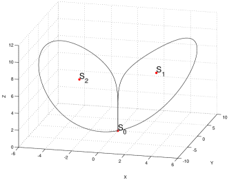
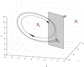
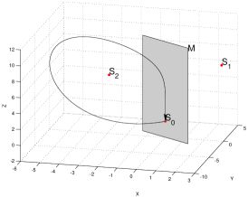
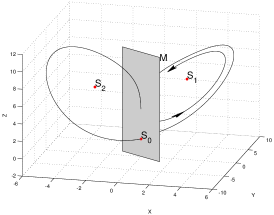
Let us fix the parameters: and (such values were considered in Glukhovskii and Dolzhanskii (1980)). For there is no intersection of the trajectory with the plane (see Fig. 3a) and for the intersection occurs (see Fig. 3c). So, there exists an intermediate value for which one can get the approximation of homoclinic orbit (see Fig. 3b). Note that the approximation for the symmetric homoclinic orbit can be obtained by the choose in the computational procedure the symmetric (with respect to ) initial data (see Fig. 2). From an analytical point of view, the existence of homoclinic trajectory can be justified by Fishing principle Leonov (2012, 2013, 2014). The Fishing principle is based on the construction of a special two-dimensional manifold such that the separatrix of the saddle point intersects or does not intersect the manifold for two different values of a system parameter. The continuity implies the existence of some intermediate value of the parameter for which the separatrix touches the manifold. According to construction the only possibility for separatrix is to touch the saddle and thus, one can numerically localize the birth of the homolcinic orbit by changing the variable parameter.
III Chaotic attractor in the Lorenz-like system
III.1 Local stability analysis and computation of attractors
Let us study the stability of equilibria , of system (2). By the Routh-Hurwitz criterion, one can get the following
Proposition 1
. If and the parameters and satisfy the inequality
| (5) |
where
then the equilibria are stable.
Let us choose the parameter and, as in Glukhovskii and Dolzhanskii (1980), construct the domains of stability of the equilibria of system (2) in dependence on the values of parameters and . Then inequality (5) takes the form
| (6) |
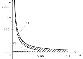
For , where , there are three real roots: , for two real roots: and , and for one real root: .
Thus, for the equilibria are stable for and and they are unstable in the converse case; for the equilibria are stable for (see, Fig. 4).
An oscillation in a dynamical system can be easily localized numerically if the initial conditions from its open neighborhood lead to the long-time behavior that approaches the oscillation. Thus, from a computational point of view it is natural to suggest the following classification of attractors, based on the simplicity of finding the basin of attraction in the phase space:
III.2 Self-excited attractor in the Lorenz-like system
For a self-excited attractor its basin of attraction is connected with an unstable equilibrium and, therefore, self-excited attractors can be localized numerically by the standard computational procedure, in which after a transient process a trajectory, started from a point of an unstable manifold in a neighborhood of an unstable equilibrium, is attracted to the state of oscillation and traces it. Thus self-excited attractors can be easily visualized.
Using the constructed domain of stability (4), one considers a qualitative behavior of trajectories of system (2) for the fixed , , and . For system (2) the parameter is chosen.
For the above parameters the eigenvalues of equilibria of system (2) are the following
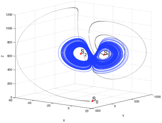
Thus, the equilibrium is a saddle and are saddle-focuses. Having taken an initial point on the unstable manifold of one of equilibria (Fig. 5), one can easily be vizualized a self-excited chaotic attractor by standard computational procedure.
For the equilibria become stable and the trajectories, starting from the neighborhood of equilibrium , are attracted to or . The question arises whether there exists a hidden chaotic attractor in system (2) for such values of parameters? Next for the computation of hidden attractor in system (2) a special numerical procedure is considered.
III.3 Hidden attractor in the Lorenz-like system
For a hidden attractor its basin of attractor is not related with unstable equilibria. The hidden attractors, for example, are the attractors in the systems with no equilibria or with only one stable equilibrium (a special case of multistable systems and coexistence of attractors). Recent examples of hidden attractors can be found in (Leonov et al., 2014; Zhusubaliyev and Mosekilde, 2014; Pham et al., 2014a, b; Wei et al., 2014a; Li and Sprott, 2014; Wei et al., 2014b; Kuznetsov et al., 2014a; Li et al., 2014; Zhao et al., 2014; Lao et al., 2014; Chaudhuri and Prasad, 2014). Multistability is often an undesired situation in many applications but the coexisting self-excited attractors can be found by the standard computational procedure. In contrast, there is no regular way to predict the existence or coexistence of hidden attractors in system. Note that one cannot guarantee the localization of attractor by the integration of trajectories with random initial data (especially for multidimensional systems) since its basin of attractor may be very small.
One of the effective methods for numerical localization of hidden attractors in multidimensional dynamical systems is based on a homotopy and numerical continuation: it is necessary to construct a sequence of similar systems such that for the first (starting) system the initial data for numerical computation of oscillating solution (starting oscillation) can be obtained analytically, e.g, it is often possible to consider the starting system with self-excited starting oscillation. Then the transformation of this starting oscillation is tracked numerically in passing from one system to another.
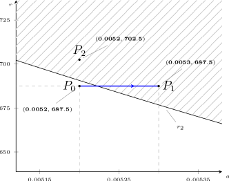
Let us construct on the plane a line segment, intersecting a boundary of the domain of stability of the equilibria , (see Fig. 6). Let us choose the point : , as the finite point of the line segment. To these parameters correspond the following eigenvalues of the equilibria of system (2):
It means that the equilibria become stable focus-nodes.
Let us choose the point
as the initial point of the line segment. This point corresponds to the parameters for which in system (2) there exists a self-excited attractor, which can be computed by the standard procedure. Then for the considered line segment a sufficiently small partition step is chosen and a chaotic attractor in the phase of system (2) space at each iteration of the procedure is computed. The last computed point at each step is used as the initial point for the computation of the next step.
Our experiment has iterations and the partition step equals , respectively. At each iteration for the current trajectory that describes the attractor one computes the largest Lyapunov exponent () Benettin et al. (1980a) and the Lyapunov dimension () Kaplan and Yorke (1979); Boichenko et al. (2005) 111 There are two widely used definitions of Lyapunov exponents: the upper bounds of the exponential growth rate of the norms of linearized system solutions and the upper bounds of the exponential growth rate of the singular values of linearized system fundamental matrix. While in typical case these two definitions gave the same values, for a given system they may be different and there are examples in which Benettin algorithm Benettin et al. (1980b) (see, e.g., its MATLAB implementation Siu (1998)) fails to compute the correct values (see the discussion in Kuznetsov et al. (2014b)).
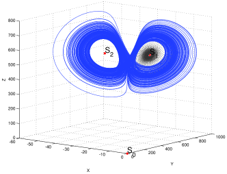
Thus, for the selected path and selected partition it is possible to visualize a hidden attractor of system (2) (see Fig. 7).
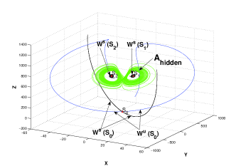
Remark that hidden attractor does not exist for all points of the shaded domain in Fig. 6. E.g., there is no chaotic attractor for the point : , .
IV Conclusions
In the present work by numerical methods the scenario of transition to chaos in physical model (2), describing a flow of rotating fluid convection inside the ellipsoid under horizontal heating, is demonstrated. Similarly to scenario in the classical Lorenz system, in system (2) a homoclinic trajectory and self-excited chaotic attractor are constructed. However, unlike the Lorenz system for system (2) one is able to localize numerically a hidden attractor.
Acknowledgements.
This work was supported by Russian Scientific Foundation (project 14-21-00041) and Saint-Petersburg State University.References
- Glukhovskii and Dolzhanskii (1980) A. B. Glukhovskii and F. V. Dolzhanskii, ‘‘Three-component geostrophic model of convection in a rotating fluid,’’ Academy of Sciences, USSR, Izvestiya, Atmospheric and Oceanic Physics 16, 311–318 (1980), (Translation).
- Lorenz (1963) E. N. Lorenz, ‘‘Deterministic nonperiodic flow,’’ J. Atmos. Sci. 20, 130–141 (1963).
- Rabinovich (1978) M. I. Rabinovich, ‘‘Stochastic self-oscillations and turbulence,’’ Uspekhi Fizich. Nauk 125, 123–168 (1978), (in Russian).
- Leonov and Boichenko (1992) G. A. Leonov and V. A. Boichenko, ‘‘Lyapunov’s direct method in the estimation of the Hausdorff dimension of attractors,’’ Acta Applicandae Mathematicae 26, 1–60 (1992).
- Pikovski et al. (1978) A. S. Pikovski, M. I. Rabinovich, and V. Yu. Trakhtengerts, ‘‘Onset of stochasticity in decay confinement of parametric instability,’’ Sov. Phys. JETP 47, 715–719 (1978).
- Xie and Zhang (2003) F. Xie and X. Zhang, ‘‘Invariant algebraic surfaces of the Rabinovich system,’’ J. Phys. A 36, 499–516 (2003).
- Zhang (2003) X. Zhang, ‘‘Integrals of motion of the Rabinovich system,’’ J. Phys. A 33, 5137–5155 (2003).
- Zhang et al. (2014) F. Zhang, Ch. Mu, L. Wang, X. Wang, and Yao X., ‘‘Estimations for ultimate boundary of a new hyperchaotic system and its simulation,’’ Nonlinear Dynamics 75, 529–537 (2014).
- Denisov (1989) G. G. Denisov, ‘‘On the rigid body rotation in resisting medium,’’ Izv. Akad. Nauk SSSR: Mekh. Tverd. Tela 4, 37–43 (1989), (in Russian).
- Glukhovsky (1982) A. B. Glukhovsky, ‘‘Nonlinear systems in the form of gyrostat superpositions,’’ Doklad. Akad. Nauk SSSR 266, 816–820 (1982), (in Russian).
- Glukhovsky (1986) A. B. Glukhovsky, ‘‘On systems of coupled gyrostat in problems of geophysical hydrodynamics,’’ Izv. Akad. Nauk SSSR: Fiz. Atmos. i Okeana 22, 701–711 (1986), (in Russian).
- Zaks et al. (1983) M. A. Zaks, D. V. Lyubimov, and V. I. Chernatynsky, ‘‘On the influence of vibration upon the regimes of overcritical convection,’’ Izv. Akad. Nauk SSSR: Fiz. Atmos. i Okeana 19, 312–314 (1983), (in Russian).
- Dovzhenko and Dolzhansky (1987) V. A. Dovzhenko and F. V. Dolzhansky, Generating of the vortices in shear flows. Theory and experiment (Nauka, Moscow, 1987) pp. 132–147, (in Russian).
- Evtimov et al. (2000) S. Evtimov, S. Panchev, and T. Spassova, ‘‘On the Lorenz system with strengthened nonlinearity,’’ Comptes rendusde l’Académie bulgare des Sciences 53, 33–36 (2000).
- Panchev et al. (2007) S. Panchev, T. Spassova, and N. K. Vitanov, ‘‘Analytical and numerical investigation of two families of lorenz-like dynamical systems,’’ Chaos, Solitons and Fractals 33, 1658–1671 (2007).
- Liao et al. (2010) B. Liao, Y. Y. Tang, and L. An, ‘‘On lorenz-like dynamic systems with strengthened nonlinearity and new parameters,’’ International Journal of Wavelets, Multiresolution and Information Processing 8, 293–311 (2010).
- Akhtanov et al. (2013) S. N. Akhtanov, Z. Zh. Zhanabaev, and M. A. Zaks, ‘‘Sequences of gluing bifurcations in an analog electronic circuit,’’ Physics Letters A 377, 1621–1626 (2013).
- Boichenko et al. (2005) V. A. Boichenko, G. A. Leonov, and V. Reitmann, Dimension theory for ordinary differential equations (Teubner, Stuttgart, 2005).
- Sparrow (1982) C. Sparrow, The Lorenz Equations: Bifurcations, Chaos and Strange Attractors, Applied Mathematical Sciences, Vol. 41 (Springer-Verlag, New-York, 1982).
- Leonov (2012) G. A. Leonov, ‘‘General existence conditions of homoclinic trajectories in dissipative systems. Lorenz, Shimizu–Morioka, Lu and Chen systems,’’ Physics Letters A 376, 3045–3050 (2012).
- Leonov (2013) G.A. Leonov, ‘‘Shilnikov chaos in Lorenz-like systems,’’ International Journal of Bifurcation and Chaos 23, 1350058 (2013).
- Leonov (2014) G. A. Leonov, ‘‘Fishing principle for homoclinic and heteroclinic trajectories,’’ Nonlinear Dynamics 78, 2751–2758 (2014).
- Kuznetsov et al. (2010) N. V. Kuznetsov, G. A. Leonov, and V. I. Vagaitsev, ‘‘Analytical-numerical method for attractor localization of generalized Chua’s system,’’ IFAC Proceedings Volumes (IFAC-PapersOnline) 4, 29–33 (2010).
- Leonov et al. (2011) G. A. Leonov, N. V. Kuznetsov, and V. I. Vagaitsev, ‘‘Localization of hidden Chua’s attractors,’’ Physics Letters A 375, 2230–2233 (2011).
- Leonov et al. (2012) G. A. Leonov, N. V. Kuznetsov, and V. I. Vagaitsev, ‘‘Hidden attractor in smooth Chua systems,’’ Physica D: Nonlinear Phenomena 241, 1482–1486 (2012).
- Leonov and Kuznetsov (2013) G. A. Leonov and N. V. Kuznetsov, ‘‘Hidden attractors in dynamical systems. From hidden oscillations in Hilbert-Kolmogorov, Aizerman, and Kalman problems to hidden chaotic attractors in Chua circuits,’’ International Journal of Bifurcation and Chaos 23 (2013), 10.1142/S0218127413300024, art. no. 1330002.
- Leonov et al. (2014) G. A. Leonov, N. V. Kuznetsov, M. A. Kiseleva, E. P. Solovyeva, and A. M. Zaretskiy, ‘‘Hidden oscillations in mathematical model of drilling system actuated by induction motor with a wound rotor,’’ Nonlinear Dynamics 77, 277–288 (2014).
- Zhusubaliyev and Mosekilde (2014) Z.T. Zhusubaliyev and E. Mosekilde, ‘‘Multistability and hidden attractors in a multilevel DC/DC converter,’’ Mathematics and Computers in Simulation (2014), doi:10.1016/j.matcom.2014.08.001.
- Pham et al. (2014a) V.-T. Pham, S. Jafari, C. Volos, X. Wang, and S.M.R.H. Golpayegani, ‘‘Is that really hidden? The presence of complex fixed-points in chaotic flows with no equilibria,’’ International Journal of Bifurcation and Chaos 24 (2014a), 10.1142/S0218127414501466, art. num. 1450146.
- Pham et al. (2014b) V.-T. Pham, F. Rahma, M. Frasca, and L. Fortuna, ‘‘Dynamics and synchronization of a novel hyperchaotic system without equilibrium,’’ International Journal of Bifurcation and Chaos 24 (2014b), art. num. 1450087.
- Wei et al. (2014a) Z. Wei, R. Wang, and A. Liu, ‘‘A new finding of the existence of hidden hyperchaotic attractors with no equilibria,’’ Mathematics and Computers in Simulation 100, 13–23 (2014a).
- Li and Sprott (2014) C. Li and J. C. Sprott, ‘‘Coexisting hidden attractors in a 4-D simplified Lorenz system,’’ International Journal of Bifurcation and Chaos 24 (2014), 10.1142/S0218127414500345, art. num. 1450034.
- Wei et al. (2014b) Z. Wei, I. Moroz, and A. Liu, ‘‘Degenerate Hopf bifurcations, hidden attractors and control in the extended Sprott E system with only one stable equilibrium,’’ Turkish Journal of Mathematics 38, 672–687 (2014b).
- Kuznetsov et al. (2014a) A.P. Kuznetsov, S.P. Kuznetsov, E. Mosekilde, and N.V. Stankevich, ‘‘Co-existing hidden attractors in a radio-physical oscillator system,’’ Journal of Physics A: Mathematical and Theoretical (2014a), accepted.
- Li et al. (2014) Q. Li, H. Zeng, and X.-S. Yang, ‘‘On hidden twin attractors and bifurcation in the Chua’s circuit,’’ Nonlinear Dynamics 77, 255–266 (2014).
- Zhao et al. (2014) H. Zhao, Y. Lin, and Y. Dai, ‘‘Hidden attractors and dynamics of a general autonomous van der Pol-Duffing oscillator,’’ International Journal of Bifurcation and Chaos 24 (2014), 10.1142/S0218127414500801, art. num. 1450080.
- Lao et al. (2014) S.-K. Lao, Y. Shekofteh, S. Jafari, and J.C. Sprott, ‘‘Cost function based on Gaussian mixture model for parameter estimation of a chaotic circuit with a hidden attractor,’’ International Journal of Bifurcation and Chaos 24 (2014).
- Chaudhuri and Prasad (2014) U. Chaudhuri and A. Prasad, ‘‘Complicated basins and the phenomenon of amplitude death in coupled hidden attractors,’’ Physics Letters, Section A: General, Atomic and Solid State Physics 378, 713–718 (2014).
- Benettin et al. (1980a) G. Benettin, L. Galgani, A. Giorgilli, and J.-M. Strelcyn, ‘‘Lyapunov characteristic exponents for smooth dynamical systems and for hamiltonian systems; a method for computing all of them. part 1: Theory. part 2: Numerical application,’’ Meccanica 15, 9–30 (1980a).
- Kaplan and Yorke (1979) J. L. Kaplan and J. A. Yorke, ‘‘Chaotic behavior of multidimensional difference equations,’’ in Functional Differential Equations and Approximations of Fixed Points (Springer, Berlin, 1979) pp. 204–227.
- Benettin et al. (1980b) G. Benettin, L. Galgani, A. Giorgilli, and J.-M. Strelcyn, ‘‘Lyapunov characteristic exponents for smooth dynamical systems and for hamiltonian systems. A method for computing all of them. Part 2: Numerical application,’’ Meccanica 15, 21–30 (1980b).
- Siu (1998) S. Siu, ‘‘Lyapunov Exponents Toolbox (LET),’’ http://www.mathworks.com/matlabcentral/fileexchange/233-let (1998).
- Kuznetsov et al. (2014b) N. V. Kuznetsov, T.A. Alexeeva, and G. A. Leonov, ‘‘Invariance of Lyapunov characteristic exponents, Lyapunov exponents, and Lyapunov dimension for regular and non-regular linearizations,’’ arXiv:1410.2016v2 (2014b).
- Leonov and Mokaev (2015) G. A. Leonov and T. N. Mokaev, ‘‘Estimation of attractor dimension for differential equations of convection in rotating fluid,’’ International Journal of Bifurcation and Chaos (2015), (submitted).