Orbital Motion During Gravitational Lensing Events

Abstract

Gravitational lensing events provide unique opportunities to discover and study planetary systems and binaries. Here we build on previous work to explore the role that orbital motion can play in both identifying and learning more about multiple-mass systems that serve as gravitational lenses. We find that a significant fraction of planet-lens and binary-lens light curves are influenced by orbital motion. Furthermore, the effects of orbital motion extend the range of binaries for which lens multiplicity can be discovered and studied. Orbital motion will play an increasingly important role as observations with sensitive photometry, such as those made by the space missions Kepler, Transiting Exoplanet Survey Satellite, (TESS ), and WFIRST discover gravitational lensing events. Similarly, the excellent astrometric measurements made possible by GAIA will allow it to study the effects of orbital motion. Frequent observations, such as those made possible with the Korean Microlensing Telescope Network, KMTNet will also facilitate the study of orbital motion during gravitational lensing events. Finally, orbital motion will typically play a significant role in the characteristics of lensing events in which the passage of a specific nearby star in front of a background star can be predicted.

1 Introduction

1.1 The Importance of Orbital Motion During Lensing Events

Many of the masses serving as lenses in gravitational lensing events are planetary systems, binaries, or higher-order multiples. As the lensing events proceed, the bodies constituting the lens system continue to orbit each other. Orbital motion changes the magnification pattern as the lens passes in front of the lensed source. When the event lasts longer than the time required for a significant change in orbital phase, the light curve may exhibit unique characteristics.

In this paper, we establish that a significant fraction of all light curves exhibiting evidence of lens multiplicity should also provide detectable signatures of orbital motion. Our focus is on identifying the characteristics of those systems for which orbital motion produces detectable features in gravitational lensing light curves, The “characteristics” we consider include intrinsic properties (mass and orbital properties), and also the placement of the binary relative to us (distance and the orientation of its orbit). For systems likely to exhibit the effects of orbital motion, we study the range of possible effects and consider how these effects can be identified and studied. Search for orbital motion will make lensing observations more effective in discovering binaries and planetary systems. These searches will become more successful as we move to an era in which (1) lensing events caused by nearby stars can be predicted (Lépine & DiStefano 2012), (2) the photometric and astrometric precision of several space missions can be applied to lensing studies (Kepler (Borucki & Koch 2012), TESS (Ricker et al. 2014), WFIRST (Yee et al. 2014), GAIA (Proft et al. 2011, Dominik & Sahu 2000), and (3) round-the-clock high-cadence sampling commences from the ground KMTNet (Henderson et al. 2014) .

1.2 Historical Background

Lensing light curves can display dramatic changes from the point-lens form when the lens is a binary or planetary system. Early investigations of lens multiplicity focused on cases in which the event duration is so much shorter than the orbital period that orbital motion produced subtle or negligible effects, Indeed, evidence of rotation discovered so far has been found in a handful of systems that have experienced modest changes in orbital phase during the lensing event.

Di Stefano (2008) considered the case in which the orbital period is comparable to or smaller than the event duration. In this cases, close approaches to a binary lens can produce light curves that are far more complex than the most intricate light curves generated by a non-rotating binary lens. The top panel of Figure 1 of that paper shows the result of a head-on approach at low speed to a double brown-dwarf binary. The event exhibits $6$ caustic crossings and $5$ additional obvious peaks. Although the binary completed approximately two orbits during the detectable portion of the event, the light-curve pattern is not obviously periodic, but there is some evidence of quasiperiodic behavior in the low-magnification wings of the light curve. It is not clear whether such a light curve would have been identified as a candidate lensing event, particularly in the earlier incarnations of the lensing monitoring teams. Of course the approach between source and lens in this case was special, in order that the source would pass over regions with highly perturbed patterns of magnification. In the more typical cases considered in this paper, the perturbations are milder. Nevertheless, the complexity of the light curves and model fits increases when the effects of orbital period, including possibly several objects in orbit, orientation on the sky play significant roles.

Di Stefano & Night (2008) extended the study of orbital rotation during events to the case of planets. They showed earby planets orbiting in the habitable zones of their stars, the ratio of orbital period to event duration is also favorable for the detection of orbital motion.

To study the effects of a range of ratios between the event duration and orbital period, we utilize the concepts of the Einstein angle and the Einstein radius. When the source, lens, and observer are perfectly aligned, the image of the source is a ring whose angular radius is referred to as the Einstein angle, $\theta_{E}$. When the alignment is not exact, there are two images, whose separation is comparable to $\theta_{E}.$

When the angular separation between the distant source and intervening lens is equal to $\theta_{E},$ the total magnification is $34\%$. The Einstein radius as projected onto the lens plane is just $R_{E}=\theta_{E}D_{L},$ where $D_{L}$ is the distance to the lens.

$$R_{E}=0.6\,{\rm AU}\,\sqrt{\Big{(}{{M}\over{M_{\odot}}}\Big{)}\Big{(}{{D_{L}}\over{50\,{\rm pc}}}\Big{)}\Big{(}1-\frac{D_{L}}{D_{S}}\Big{)}},$$ (1)

where $M,$ is the total mass of the lens and $D_{S}$ is the distance to the lensed source. The effects of lens binarity are most pronounced when $a,$ the projected separation between the binary components is comparable to $R_{E}.$ It is convenient to define $\alpha=a/R_{E}.$ Many of the binaries and planetary systems observed as lenses so far tend to have values of $\alpha$ between roughly $0.2$ and  $2.0$.

For a solar-mass lens located halfway between us and the Bulge, $R_{E}\approx 5$ AU. The orbital period for binary lenses with $\alpha\approx 1$ can therefore be several years. In contrast, typical event durations have been on the order of days, weeks, or months. Under these circumstances, the orbital phase should not change very much during an event, and indeed, with hundreds of binary-lens events identified, phase shifts have been measured in only a handful of cases, and the values tend to be small (Dominik 1998, Albrow et al. 2000, An et al. 2000).

Dominik (1998) considered the effects of orbital rotation, including cases in which either the lens or source is a binary. He found that, of these effects, binary-lens rotation produces the most significant light-curve perturbations. He identified an acceptable model fit to the DUO#2 event that includes the effect of rotation, but the phase change during the event was small, since the Einstein radius crossing time was $6.4$ days, while the binary orbital period was $85.4$ days. Ioka et al. (1999) found that Kepler rotation should be significant for binary lenses in the Magellanic Clouds, although orbital effects were not needed to fit MACHO LMC-9, a binary-lens event. Dubath et al. (2008) considered fast-rotating lenses, but miscomputed the light curves by not including the important non-linear effects associated with binary lenses.

More recently, Penny et al. (2011a) carried out a simulation of microlensing events produced by the Galactic binary population, and also Penny et al. 2011b computed the detection efficiency for orbital effects. Unsurprisingly, they find that averaged over all relevant parameters (distances, binary periods and separations, relative velocities, etc.), the detectable fraction is considerably lower than 0.1% This is of course consistent with the general consensus that such events are very rare, which is why the effects of orbital motion in microlensing were largely ignored for so long. More importantly, Penny et al. explored the effects of different microlensing parameters on the rate of orbital motion detection. However, because their study focused on population averages, the interpretation of their results is not always straight-forward, since it depends on the authors’ choices for the distributions of critical parameters (e.g. lens distances, periods, etc.). In any case, binary population calculations are complicated by the need to incorporate stellar and binary evolution as well as planetary systems. Calculations conducted to calculate the rate of Type Ia supernovae, for example, give different results when performed by different groups (Nelemans et al. 2013). Furthermore, there is evidence that even the “initial conditions”, corresponding to the range of orbital periods, masses, mass ratios, and eccentricities in primordial binaries, need to be better established (Moe & Di Stefano 2013a, 2013b).

In this paper we therefore take a different approach. We identify the sets of system and event parameters that allow orbital motion to significantly influence the form of the light curve. We study the effects. We then consider a range of physical and mathematical symmetries that identify a huge range of systems expected to produce similar light curves. Some of these systems have low mass stars, others are high-mass binaries. Some have short orbital periods, others orbital periods of hundreds of days. Some are near to us, and some ar close to the source star. We thereby show that the effects of orbital motion are likely to be ubiquitous. We show that a calculational method, developed by Guo et al. (2011), is needed to search for and consistently find evidence for it, and to reliably measure binary orbital periods.

1.3 Plan of the Paper

In §2 we identify the regions of the parameter space for planetary and binary systems in which orbital motion should influence the lensing signatures. We find that for some sets of event parameters, the effects of orbital motion can be detected even for binary lenses with orbital periods of tens to hundreds of days. Furthermore, the effects of lensing and the binary nature of the lens can be more detectable when the light curve carries information about orbital motion. We illustrate these results by considering a binary located at a fixed distance $D_{L}$ from the observer, computing the effects of rotation for a range of orbital separations.

In §3 we turn to a set of five instructive examples with a broad range of physical properties to demonstrate the connection between the rotating geometry of the lens and the lensing signature. Although the number of systems we consider is relatively small, we show that each represents a large set of binaries. Section 4 is devoted to our conclusions. We find that a large fraction of those planetary systems and binaries for which the lensing event provides evidence of a companion, the light curve is also significantly influenced by orbital motion. Furthermore, the effects of orbital motion extend the range of values of the orbital separation for which lens multiplicity can be discovered, and teach us more about the multiple system that served as a lens. We conclude with a discussion of how observational studies can identify more events exhibiting orbital motion.

2 The Effects of Orbital Motion

2.1 Detecting Evidence of Binarity: Static Lenses

We start by considering a point-like lens of mass $M.$ The lens position defines the center of a set of circular isomagnification contours projected onto the sky. If we define $u$ to be the projected distance between the lens and the background source, expressed in units of the Einstein radius, $R_{E},$ the magnification depends only on the value of $u$: $A[u(t)]=(u^{2}+2)/(u\sqrt{u^{2}+4})$. Because the lens has no structure, all angles of approach are equivalent, and the lensing light curve is symmetric about a peak magnification that occurs at the time of closest approach between the lens and a background source of light. Lensing model fits to the light curve provide the value of the distance of closest approach, the time of closest approach, the baseline magnitude, and a time duration $\tau_{E},$ defined to be the time required for the lens-source distance to change by $2\,R_{E}.$ The value of $\tau_{E}$ is the only measurable quantity that depends on the lens mass, $M.$ Measuring $\tau_{E}$ does not, however, provide a unique measure of the lens mass, because value of $\tau_{E}$ is also determined by the distances to the lens and source ($D_{L}$ and $D_{S}$, respectively), and the value $v$ of the relative transverse speed. The lensing solution is therefore highly degenerate.

Lens binarity breaks the axisymmetry, and expresses itself through deviations in the isomagnification contours. When the path of a distant star passes behind regions that deviate from the point-lens pattern, the lensing light curve exhibits distinctive features. Because these features introduce a physical scale, they can help to break the degeneracy discussed above. For example, sometimes finite-source-size effects can be detected when binary-lens effects introduce short-lived deviations; these can allow us to measure the size of $\theta_{E},$ and to thereby directly relate the mass of the lens to its distance from us.

The spatial structure of the deformations, and therefore the shapes of the light curves depend on the binary’s physical characteristics. For static binaries the two key quantities are the mass ratio $q$ between the binary components and the projected orbital separation, $a$. We define $q=M_{2}/M_{1},$ where $M_{2}<M_{1}$. Lensing is not directly sensitive to the 3-dimensional orbital separation, but instead depends on the value of the $a,$ the orbital separation projected onto the plane of the sky. The effects are determined by the ratio $\alpha=a/R_{E}.$

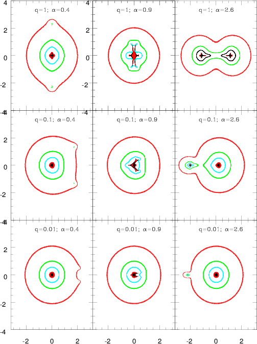
Figure 1: Isomagnification regions for 9 binary lenses. Outer contour (red): A=2.05. Proceeding inward, $A=1.34$ along the green contours, and $A=2$ along the cyan contours. Inner points in red (black) mark regions in which the magnification is larger than 5 (10). The value of $\alpha$ increases from left to right and the value of $q$ decreases from top to bottom. Di Stefano (2012) considers smaller values of $\alpha.$

For a given value of $\alpha,$ the effects of binarity on the isomagnification contours are small for values of $q$ in the range typical of planets, but the linear dimensions of the regions in which there are significant perturbations increase with increasing $q$. Some examples are shown in Figure 1, with the patterns in the top, middle, and bottom rows corresponding to $q=1,,0.1,$ and $0.01,$ respectively.

For a given value of $q,$ the size of the region in which there are significant perturbations is typically largest for $\alpha\sim 1.$ As $\alpha$ increases above unity, the isomagnification contours begin to mimic the contours expected from two separate lenses. As $\alpha$ decreases below unity, the region with large photometric deviations from the point-lens form shrinks. The progression from small to large $\alpha$ can seen by scanning from left to right in each row of Figure 1.

Because the deviations shrink for smaller values of $\alpha,$ most previous investigations have not explicitly considered small $\alpha.$ Nevertheless, at small $\alpha,$ there is a region of perturbations at a distance roughly equal to $1/\alpha$ from the center of mass (Di Stefano 2012, Di Stefano & Night 2008). This is illustrated in the left-hand panels of Figure 1 and is addressed in detail for planets in Di Stefano 2012. We also include examples of small-$\alpha$ binaries in this paper.

2.2 Relating the orbital period to the lensing parameters

The value of the orbital period, $P,$ depends on the value of the total system mass, $M,$ which is also the mass that enters into the expressions for the Einstein radius, $R_{E}$, and for the Einstein diameter crossing time, $\tau_{E}$. The value of $P$ also depends on the size, $a_{s}$ of the semimajor axis. If we define $\alpha_{s}=a_{s}/R_{E},$ then

$$P=1~{}{\rm yr}~{}\,\Big{(}\alpha_{s}\Big{)}^{\frac{3}{2}}\,\Bigg{(}{\frac{R_{E}}{AU}}\Bigg{)}^{\frac{3}{2}}\,\Bigg{(}\frac{M_{\odot}}{M}\Bigg{)}^{\frac{1}{2}}$$ (2)

It is not, however, $\alpha_{s}$ that determines the shapes of the isomagnification contours. Instead, it is the instantaneous value of the projected separation, expressed in units of $R_{E}$: $\alpha=a/R_{E}$. In general $\alpha=\alpha(t)=f(t)\,\alpha_{s}.$ For eccentric orbits viewed nearly face-on, $f(t)>1$ near apastron. Near periastron, or for inclined orbits $f(t)<1$. It is convenient to express $P$ as follows.

$$P=170\,{\rm days}\,\alpha_{s}^{3/2}\Bigg{[}{{M}\over{M_{\odot}}}\,\Bigg{(}\frac{D_{L}}{50\,{\rm pc}}\Bigg{)}^{3}(1-\frac{D_{L}}{D_{S}})^{3}\Bigg{]}^{1\over 4}$$ (3)

In order for the effects of orbital motion to play a role in altering the shape of the light curve, the binary axis must rotate significantly while the event is in progress. We must therefore compare the time scale of the event to the orbital period. The time scale for photometric events is set by the value of $\tau_{E}=2\,R_{E}/v,$ where $v$ is the relative transverse velocity of the source in the frame of the lens.

$$\tau_{E}=41.6\ {\rm days}\Bigg{(}{{M}\over{M_{\odot}}}\Bigg{)}^{{1}\over{2}}\Bigg{(}{{D_{L}}\over{50\,{\rm pc}}}\,(1-x)\Bigg{)}^{{1}\over{2}}\Bigg{(}{{50\,{\rm km/s}}\over{v}}\Bigg{)},$$ (4)

which combined with Eq. (3) gives us the timescale ratio

$${{\tau_{E}}\over{P}}={{2.73}}\,\Big{(}{{0.2}\over{\alpha_{s}}}\Big{)}^{{3}\over{2}}\,\Big{(}{{50\,\rm{km/s}}\over{v_{T}}}\Big{)}\,\Bigg{[}{{M}\over{M_{\odot}}}\,{{50\,{\rm pc}}\over{{D_{L}}\,(1-x)}}\Bigg{]}^{1\over 4}.$$ (5)

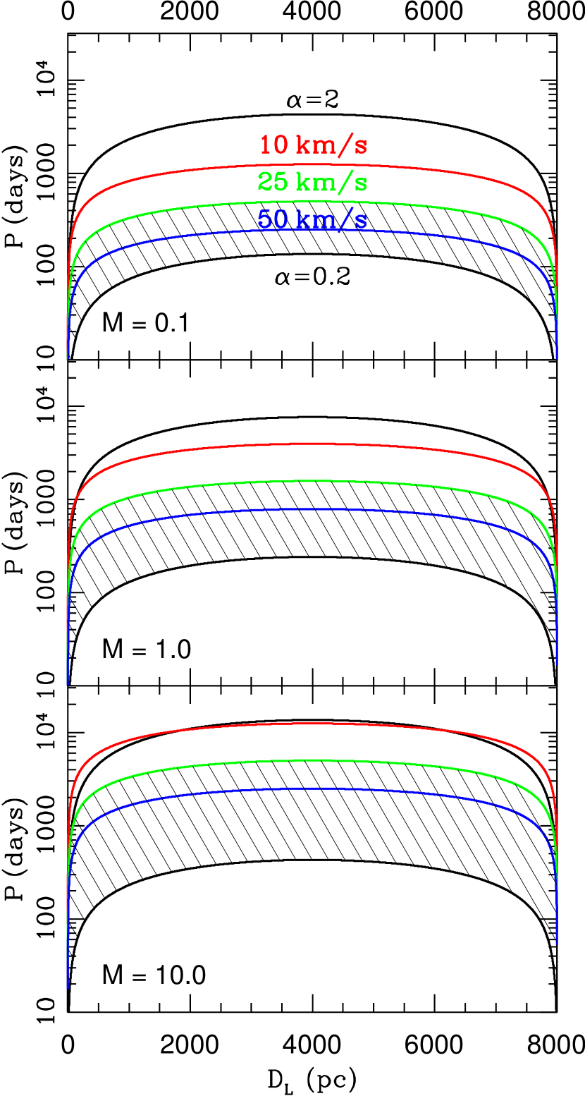
Figure 2: Ranges of orbital periods, as a function of lens distance, for which lens binarity can be reliably detected; we take $D_{S}=8$ kpc. Top panel: $M=0.1\,M_{\odot}$; Middle panel: $M=1.0\,M_{\odot}$; Bottom panel: $M=10.\,M_{\odot}$. In each panel, $P-D_{L}$ relationship shown in the uppermost (lowermost) black curves is computed by using Eq. 3 for $\alpha=2$ ($\alpha=0.2$), the approximate range of $\alpha$ for which lens binarity is detectable, even without orbital motion. The colored curves show the $P_{max}-D_{L}$ relationship (Eq. 6), each for a specific value of the relative transverse velocity (red (top): $10$ km s^-1; green (middle): $25$ km s^-1; blue (bottom): $50$ km s^-1). The region below each of these curves corresponds to the region within which the effects of orbital rotation significantly changes the light curve properties (Eq. [6]). For illustrative purposes, the hatched region shows (for the specific case of $v=25\,{\rm km/s}$) the intersection of the region where binarity is potentially detectable (even without orbital motion) with the region where orbital motion plays an important role and can significantly deform the shape of the binary-lens light curves.

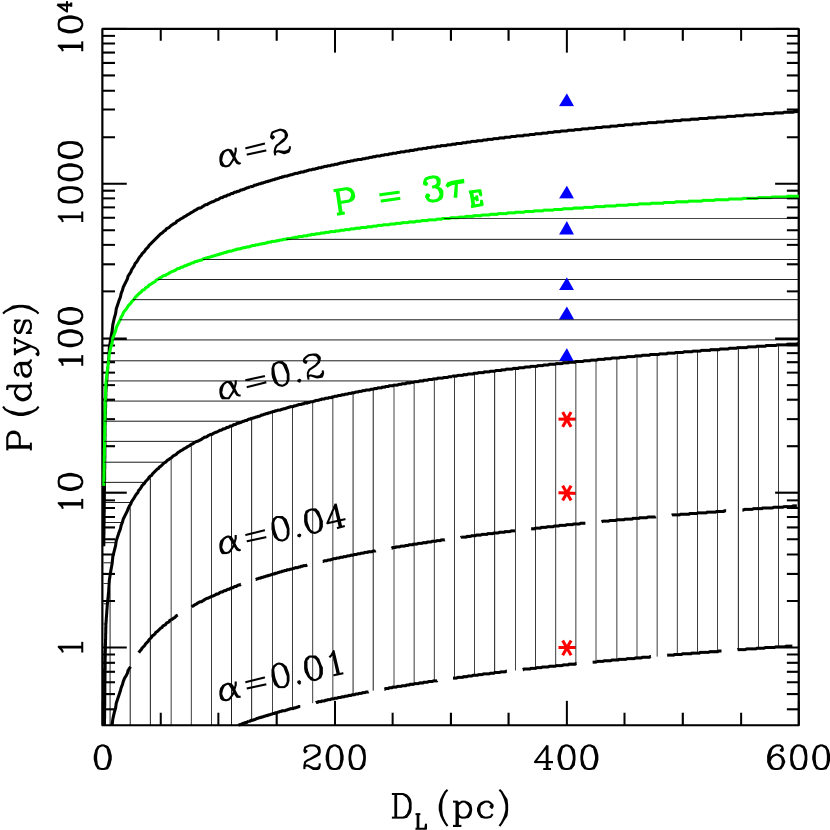
Figure 3: Maximum and minimum binary periods (as in Figure 2) for nearby lenses with total mass $1M_{\odot}$ and relative velocity $v=25\,{\rm km/s}$. The region with horizontal shading is the same as the shaded region in Figure 2; here binary rotation causes very significant changes to the lightcurve. The binary lenses with periods in the region with vertical shading will show detectable rotation signatures in microlensing lightcurves observed with sensitivity better than the present $\sim 1\%$. The lightcurves for the lensing events produced by systems labeled as blue triangles and red stars are shown in Figures 4 and 5.

2.3 Detecting Evidence of Orbital Motion

The timescale ratio, ${{\tau_{E}}/{P}}$, can indeed be very small (i.e. rotation is unimportant) for large values of $\alpha$, $v$, and $D_{L}(1-x)$. However, in this section we demonstrate that the value of $\tau_{E}/P$ large enough to produce detectable effects for a wide range of binary-lens parameters. A useful criterion is that the binary should execute an orbit during an interval of time equal to $3\,\tau_{E}$. This roughly corresponds to completing an orbit during the interval when the magnification is greater than $2\%.$ Today’s ground-based missions can, in principle, track the light curve through even lower values of the magnification. Space missions can do even better. In data taken by the Kepler mission, TESS, or WFIRST, an event is potentially detectable during the interval when the lens-source separation is as large as $10\,R_{E};$ larger orbital periods would still produce significant deviations from the point-lens light curve shape.

Imposing the condition $P\lesssim 3\tau_{E}$ and using Eq. (3) to eliminate $\alpha_{s}$ in favor of $P$, implies a maximum orbital period, $P_{max}.$

$$P_{max}=125\,{\rm days}\,\left(\frac{50\,{\rm km/s}}{v}\right)\left[{{M}\over{M_{\odot}}}\,\frac{D_{L}\,(1-x)}{50\,{\rm pc}}\right]^{1/2}.$$ (6)

Note that orbital effects can be detected even when the orbital period is somewhat longer.

Figure 2 illustrates the range of orbital periods for which binary and rotational effects are potentially detectable, as a function of distance $D_{L}$ to the lens. Each panel corresponds to a specific value of the lens mass, ranging from $M=0.1\,M_{\odot}$ in the top panel to $M=10\,M_{\odot}$ in the bottom panel. In each panel, there is an upper and lower black curve showing $P$ versus $D_{L}$ for, respectively, $\alpha=2$, $\alpha=0.2$. This range of $\alpha$ roughly corresponds to the range over which lens binarity can significantly affect the shape of the light curve, even for static lenses. Thus, if a lens lies between these two curves, lens binarity is potentially detectable, even without the effects of orbital motion. It is important to note that, in the static-lens case, not every detected lensing light curve exhibits detectable evidence of binarity, even for systems for binaries in the region between $\alpha=0.2$ and $\alpha=2.$ Instead, depending on the sensitivity and cadence of the observations, there is a finite probability, often small, that lens binarity will be detectable. The probability of detecting binarity is proportional to the probability that the source track will pass behind a region with isomagnification perturbations, and is therefore proportional to the linear size of the perturbed regions. The probability increases with larger values of the mass ratio $q$, and for values of $\alpha$ close to unity.

The colored curves in each panel plot $P_{max}$ versus $D_{L}$. Each curve corresponds to a particular value of the relative velocity, indicated by the curve’s color (red: $10$ km s^-1; green: $25$ km s^-1; blue: $50$ km s^-1). For all systems located beneath a curve of a given color (whether or not $\alpha>0.2$), rotational motion is potentially detectable, since $\tau_{E}/P>3.$

Note that in each panel, the region between the green curve ($P_{max}$ for $v=25$ km s^-1) and the bottom black curve ($P$ for $\alpha=0.2$) is cross hatched. For binaries in this cross-hatched region, there is a significant probability that the light-curve perturbations associated with binarity will exhibit rotational effects.

Rotational effects can lead to the repetition of deviations, making it possible to reliably identify small deviations whose significance would otherwise be unclear. Thus, the region in which binarity can be detected may be extended to smaller values of $\alpha$ by the effects of orbital motion. This is illustrated in Figure 4.

Figure 3 is a blow-up of the small $D_{L}$ region of Figure 2, for a lens mass of $1\,M_{\odot}.$ The region with horizontal shading above the curve for $\alpha=0.2$ is the same as the shaded region in Figure 2. The region with vertical shading shows the effects of extending the systems of interest to those with lower values of $\alpha$. For these small values of $\alpha$, the expected photometric deviations from a single lens lightcurve form are tiny. However, if they can be detected (with space observations or improved ground-based photometry), the orbital motion can be so rapid that the interval during which the event occurs encompasses many orbital periods producing strong rotation signature (see Figure 5).

2.4 Effects of Orbital Motion

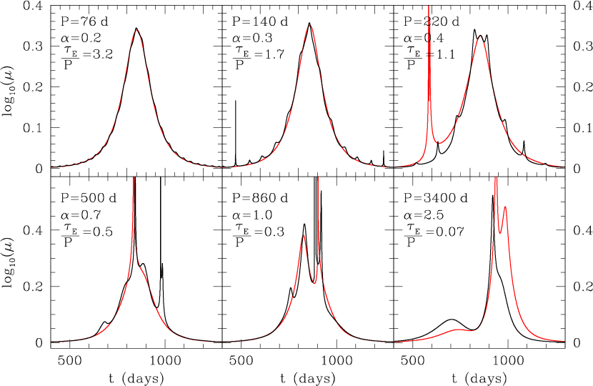
Figure 4: Shown in black is the magnification as a function of time for microlensing events produced by binary lenses with periods corresponding to the blue triangles in Figure 3. The total lens mass, mass ratio, distance, relative velocity and impact parameter are $1M_{\odot}$, $0.8,$ 400 pc, 25 km/s and $0.5R_{E}$ in all cases. The qualitative changes caused by the binary rotation are obvious for the four lowest period values. Note that periodic modulation seen for $P=76\,{\rm days}$ is at 2% level, i.e. detectable with present microlensing searches. The lightcurves for the longer period binaries still differ significantly from one would see in the limit of no rotation. This point is illustrated by the red curves, which are calculated for the same (but non-rotating) system and impact parameter; the trajectory phases were matched at the moment of closest approach.

Light Curve Morphology: The effects of orbital motion can be predicted by studying the magnification patterns shown in Figure 1. Events are produced when a source track passes behind the region near the Einstein ring of the lens. When the lens is rotating, the magnification pattern rotates and/or oscillates.

First consider a case in which the binary is face on. This is an important case, since lensing is sensitive to binarity in face-on orbits, while transit and radial-velocity methods are not. Thus, lensing studies can provide important information about binaries and planetary systems that complements what we learn through other methods. For a face-on orbit, the effects or orbital motion can be the following. A source track which, for a static lens, would have passed behind no distinctive features, will now have the features rotate into its path. In general, the number of distinctive features, such as caustic crossings and peaks and dips in the magnification, is increased by binary rotation.

Edge-on orbits are also accessible to lensing studies. In this case, the pattern of isomagnification contours doesn’t rotate, but instead it changes because the projected separation between the binary components changes with orbital phase. As the value of $\alpha$ increases and decreases, the magnification pattern oscillates. We can see this in the rows of Figure 1, by considering the sequence from left to right and then from right to left.

In general, an orbit will have an arbitrary orientation on the sky, and both rotational effects and the effects of changing values of $\alpha$ will influence the light curve. Eccentric orbits, whatever their orientation, also pass through a range of values of $\alpha$ as the orbit proceeds. Thus, whatever the orbital orientation or eccentricity, a common feature of orbiting-binary light curves is that they exhibit more structure than is typical for static binary-lens light curves. It is important to note that, even if the orbital period is too long for the light curve deviations to repeat, light curve model fits can nevertheless be used to derive the value of $P.$

Repetitions: For events that are detectable over several orbital periods, we should be able to determine that the signal is periodic and to measure the period. Tests for periodicity are complicated by (1) the time dependence of the overall magnification, (2) the shape of typical isomagnification contours, and (3) the combination of translational and orbital motion. To test for periodicity, we have conducted a Lomb-Scargle analysis on each light curve. To minimize the effects of trends in the overall magnification, we identify the best fitting point-lens light curve, and subtract this from the observed light curve. To minimize the effects of the linear structures displayed in many binary-lens isomagnification contours (which can produce two significant perturbations per orbit), we multiply measured periods by a factor of $2$. (This is not necessary for small values of $q$.) It is more challenging to correct for the contribution of translational motion. In this paper we simply show the limitations of the standard approach, and develop an improved method in a separate paper (Guo et al. 2011).

To illustrate the effects orbital motion has on microlensing lightcurves we have chosen nine representative binary lensing systems shown as blue triangles and red stars in Figure 3. Each binary has the same total mass ($1~{}M_{\odot}$) and the same mass ratio ($q=0.8$). Thus, they could be double M-dwarf systems, double white-dwarf systems (double degenerates), or white-dwarf/M-dwarf binaries. Each binary is located $400$ pc from Earth. These values of $M$ and $D_{L}$ produce $R_{E}=1.7$ AU and $\theta_{E}=R_{E}/D_{L}=4.2$ mas. To generate light curves, we set $v=25$ km/s, producing a value for the Einstein diameter crossing time of $\tau_{E}=234$ days, for all the systems and kept the distance of closest approach at $0.5\,R_{E}.$ In every case, we assumed face-on circular orbits. The only difference among our nine systems is the orbital period (or orbital separation).

Figure 4 shows (in black) the light curve for each system represented by a blue dot in Figure 3, in order of increasing period. A random orbital phase was chosen at the start of each computation. Also shown in red in each panel is the binary-lens light curve that would have been obtained if there were no orbital motion. To make a meaningful comparison, we matched the trajectory phases at the moment of closest approach

We describe each panel, starting with the smallest value of $\alpha$ and working toward higher values. On the top left is the panel for $\alpha=0.2,$ yielding an orbital period of $76$ days. The value of $\tau_{E}$ is $3.2$ times the orbital period. Thus, roughly $10$ orbital periods will pass during the time when the magnification is greater than $2\%$. By comparing the black (with rotation) and red (no rotation) curves we can clearly see the periodic modulations. However, the magnitude of the signal is low, because the distortion of the isomagnification contours for $\alpha=0.2$ is slight. Nevertheless, applying the Lomb-Scargle analysis as described above, we identify a period at a high level of significance. The value we derive, after correcting by the factor of $2$, is $70$ days, differing by less than 10% from the true period of $76$ days.

Figure 5: The three panels show the residuals from subtracting point mass lightcurves from the lightcurves produced by the binary lenses with periods shown as red stars in Figure 3. Other system parameters are the same as for Figure 4.

Figure 6: The results Lomb-Scargle periodogram analysis for three of the lightcurves shown in Figures 4 and 5. The actual periods of the binaries are indicated in the figure. Each lightcurve was sampled randomly roughly every 2 days and an uncertainty of $1\%$ and $10^{-3}\%$ was added to the data for the two longer period binaries and the short period binary, respectively. The dashed lines show the power corresponding to 98% confidence limit for the detection of periodic variability.

The middle panel in the top row shows the binary-lens light curve for $\alpha=0.3$. The larger value of $\alpha$ yields larger deviations from the non-rotating light curve. The timescale ratio $\tau_{E}/P$ is smaller for this system, so the translational motion of the binary center of mass has a stronger distorting effect on the rotational signature. Indeed, an orbital period of $123$ days recovered by the Lomb-Scargle analysis is $12\%$ lower than the true period of $140$ days. This trend continues with the third panel in the first row, for which $\alpha=0.4,$ producing an orbital period of $220$ days, just slightly smaller than the value of $\tau_{E}.$ Here, too, the periodicity is clear in the Lomb-Scargle periodogram, but the derived value is $175$ days, $20\%$ lower than the actual value.

The light curves in the bottom row of Figure 4 are generated by binaries with larger values of $\alpha,$ and, consequently, longer orbital periods. In each case, $P_{orb}>\tau_{E}$ and the periodogram analysis does not show a significant periodicity. Nevertheless, the rotational effects are large enough that the light curves for rotating binaries are significantly more complex than their corresponding static-binary counterparts, except possibly for the example with $\tau_{E}/P=0.07$.

The red dots in Figure 3 all correspond to values of $\alpha$ smaller than $0.2.$ In these cases, the deviations from the point-lens form are very small and would likely not be detected in the absence of orbital motion. The periods are short enough ($30$ days, $10$ days, $1$ day), however, that there are many orbital revolutions during a typical lensing event. As a result, the periodic nature of the photometric fluctuations is very obvious, as long as they can be detected. Figure 5 shows the residuals between the best-fit point-lens light curve in each case and the binary-lens light curve. For the cases of $30$ days and $10$ days, millimagnitude photometry would detect the deviations from the point-lens form. For the 1-day orbit, photometric sensitivity comparable to that of Kepler or the upcoming TESS mission would be needed. In all three cases, the orbital period would be extracted by the Lomb-Scargle analysis with a high degree of confidence and precision.

Figure 6 shows the results for the Lomb-Scargle analysis (with the factor of 2 correction for the period, as described above) of the three lightcurves taken from those shown in Figures 4 and 5. For the longest period system there is no convincing signal, since actual period of the binary here is more than half of the total duration of the event (which we have taken to be $3\tau_{E}$, roughly corresponding to overall magnification above $2\%$). By contrast, the middle panel shows the case where a 175-day period is detected with very high significance. This result is expected, since for this system $3\tau_{E}/P=3.3$, so the binary undergoes over 3 complete revolutions while the event is detectable. However, the detected period is not equal to the binary period of the system. This discrepancy is due to the motion of the source with respect to the binary. In Guo et al. (2011) we discuss a modified timing analysis approach that allows us to extract correct periods for such systems. Finally, the lower panel shows that there is no problem extracting the correct period for the systems where the event duration is many times higher than the orbital period (since here the motion of the source is negligible over one orbital period of the lens).

3 Exploring a wide range of systems

3.1 Systems for which orbital phase changes influence lensing light curves

In this section we display magnification maps and light curves for a small number of binaries, but begin by showing that each represents a much larger set of binaries that can generate light curves that are identical or else similar in all essential details to the ones shown here.

The crucial issue for detecting evidence of orbital motion is the ratio of the time duration of the event, to the time required for a significant change of phase to occur. We use the parameter $\tau_{E}/P$ as a proxy for this ratio, but the exact value of $\tau_{E}/P$ is not crucial, because the duration of the detectable event may be longer or shorter than $\tau_{E}$, while the required orbital phase change can be smaller than or larger than $2\,\pi$. If, for example, the photometry and sampling are good enough to allow the detection of an event over long intervals of time, or if the event is studied astrometrically, then orbital effects can be significant for relatively values of $\tau_{E}/P$ of $10$ or more.

To study a variety of situations, we consider the $5$ systems (binaries and planetary systems) listed in Table 1. Together, these systems span a range of mass ratios from unity to the planetary regime and of primary masses from those characteristic of planets or brown dwarfs to those associated with stellar-mass BHs. Although in §2 we showed that both smaller and larger values for $\alpha$ can be associated with detectable rotation-induced deviations, here we concentrate on a somewhat more limited range of $\alpha$.

System	$M_{1}/M_{\odot}$	$M_{2}/M_{\odot}$	$a$ (AU)	$P$ (days)	$D_{L}$ (pc)	$D_{S}$ (pc)	$v_{T}$ (km/s)	$\alpha$	$\tau_{E}/P$
1	0.05	0.05	0.11	42	30	8000	15	0.7	0.86
2	1.3	0.3	0.28	44	50	8000	10	0.35	6.4
3	0.8	0.002	0.17	28	30	8000	15	0.38	3.6
4	7	2	1.67	263	200	8000	25	0.44	2.0
5	0.006	0.0006	0.016	8.7	50	8000	15	0.3	1.4

Table 1: A summary of parameters for the five representative binary lens systems discussed in this section. We list primary and secondary masses, semi-major axis, orbital period, lens and source distances, relative transverse velocity $v_{T}$, $\alpha,$ and the timescale ratio $\tau_{E}/P$.

3.2 Extension to the wide range of systems represented by each individual binary

There are three ways in which a single system exhibiting the effects of phase changes can represent a larger range of different systems.

The first is that a new system can have the same orbital parameters, be located in the same place relative to us, and have the same transverse velocity, but the physical density of the lens can be different. Thus, a mass of roughly $1.3\,M_{\odot}$ may correspond to a main sequence star, a giant star, a white dwarf, or a neutron star. Systems with compact objects are common, because many lens systems are old enough that one or both components of a binary or higher-order multiple have evolved, and roughly $25\%$ of these systems will have undergone one or two epochs of mass transfer.

The second way in which an individual system represents many others, is through the similarity of the light curves to those generated by systems with somewhat different parameters. Considering, for example, the characteristics of the binary lens, Figure 1 shows that the shape of the isomagnification contours and the positions of caustics are determined by the binary mass ratio, $q$, and the separation between the binary components, $\alpha$, expressed in units of the Einstein radius. As $q$ and $\alpha$ are slowly changed from the particular values given in Table 1, the isomagnification contours also change slightly, generally morphing into shapes that will yield significantly different light curves only when the values have been changed by more than about $10\%-20\%$.

Similarly, the source path does not need to fine-tuned to produce light curves with similar characteristics. Light curves similar in their essentials (e.g., number and spacing of peaks, maximum magnification, etc.) to each of the light curves we show could have been generated when a background source follows a somewhat different path behind the lens. The distance of closest approach could have been a bit smaller or larger and/or the angle of closest approach could have been somewhat different. In general, there is a set of paths that would have produced light curves similar to the one we are studying. The details of the new set of paths might be somewhat different in small ways, but the size of the range should be comparable. Neither is fine tuning of the orbital phase required in order for the events to exhibit clear evidence of effects of rotation. The orbital phase becomes less relevant when the orbital period is short relative to the duration of the lensing event. As we will show in some of the examples in the next section, there is some difference between the cases in which the motion is prograde, versus retrograde. By prograde, we mean that the translational motion of the background source is along the same direction as the orbital motion. When the motion is retrograde, there are more opportunities for irregularities in the magnification pattern to rotate in front of the source path, increasing the effects of rotation on the light curve shape.

Finally, as discussed below, the symmetries in the basic equations mean that it is possible to transform a particular system into a very different one that will produce identical or nearly identical light curves, although generally with a rescaling of the time.

3.2.1 Similar Values of $\tau_{E}/P$ for Physically Different Binaries

To demonstrate that a range of very different physical systems can produce light curves almost identical to those that will be shown for the binaries listed in Table 1, we conducted a computational experiment. Specifically, to find binaries with similar values of $\tau_{E}/P$, we generated a large number of binary lenses. Because the shape of the light curve depends on the value of $\alpha,$ we selected only binaries with $\alpha$ having values within $0.05$ of the value shown in Table 1. Because the value of $q$ doesn’t influence the orbital period, we generated, in addition to $\alpha,$ only the relative transverse speed $v_{T},$ the total mass, $M,$ the lens distance $D_{L}.$ We considered the direction toward the Galactic Bulge, and used $D_{S}=8$ kpc.

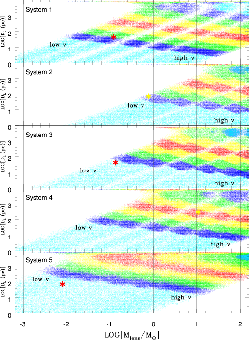
Figure 7: Points on each panel correspond to binaries that have the same value of $\tau_{E}/P$, to within $0.2$, of the value listed for the system in Table 1 that labels the panel. These binaries also have values of $\alpha$ within $0.05$ of the value listed for the system in Table 1. Points toward the left (low-velocity side) have $v_{T}$ near $10$ km s^-1; $v_{T}$ increases toward the right, to a maximum of $\sim 100$ km s^-1 on the right. Points in cyan near the bottom have orbital periods, $P$, less than $25$ days. Proceeding upward, points in dark blue have $25\,{\rm days}<P<50\,{\rm days}$; points in green have $50\,{\rm days}<P<100\,{\rm days}$. The lower and upper limits of the interval of orbital periods increase by a factor of $2$ for each subsequent colored band.

Each point in Figure 7 represents a binary lens with $\alpha$ chosen as described above and with the value of $\tau_{E}/P$ lying within $0.2$ of the value given for the corresponding system in Table 1. With values of both $\alpha$ and $\tau_{E}/P$ very close to the values used in Table 1, we are guaranteed that the binary we generated can produce a light curve almost identical to those shown in Figures 8 and 9 (System 1), Figure 10 (System 2 in the left-hand panel, System 4 in the right-hand panel); Figure 11 (System 3); Figure 12 (System 5).

The result is that a light curve with the same morphology can be produced by lenses having a wide range (several orders of magnitude) of total masses, of distances to the lens, orbital periods, and transverse speed. Furthermore, many portions of the regions covered by colored points correspond to real physical systems at various stages of evolution. To derive the points in Figure 7 this, we varied the parameters as described below.

Relative transverse speed, $v_{T}$: The value of $\tau_{E}/P$ is inversely proportional to $v_{T}$. The value of $v_{T}$ therefore plays an important role in determining whether the effects of the lens system’s orbital motion can be detected. We generated $7$ small ranges of values of $v_{T}:$ $9-11$ km s^-1, $14-16$ km s^-1, $24-26$ km s^-1, $39-41$ km s^-1, $59-61$ km s^-1, $79-81$ km s^-1, $99-101$ km s^-1. In each panel of Figure 7, points on the left-hand side (labeled “low-v”) have values of $v_{T}$ near $10$ km s^-1, and those on the right-hand side (labeled “high-v”) have values of $v_{T}$ near $100$ km s^-1. The distribution of points in each panel shows evidence of the transitions between the seven velocity ranges.

Lens mass: We selected the logarithm (to the base 10) of the mass to uniformly populate the interval between $-3.2$ (corresponding to approximately $0.6$ the mass of Jupiter) and $2.2$ (corresponding to approximately $158\,M_{\odot}$, close to the mass of the most massive star known). Bright stars, whether they are high-mass stars on the main sequence or giants, produce fewer detectable events because they are will outshine most background stars they lens by several magnitudes. Thus, the more massive stars likely to produce detectable events are stellar-mass BHs. The masses of the known stellar-mass BHs extend to roughly $35\,M_{\odot}$ (Prestwich et al. 2007) and the evolution of massive stars (as well as possible BH mergers) may produce even more massive BHs.

Distance to the lens: The functional form of $\tau_{E}/P$ exhibits a symmetry between $D_{L}/D_{S}$ and $(1-D_{L}/D_{S})$. Thus, for a fixed $D_{S},$ the value of $\tau_{E}/P$ is the same for a lens $100$ pc from us as it is for a lens $100$ pc from the source star. If, therefore, we had plotted $D_{L}$, instead of $log_{10}(D_{L})$, each panel of Figure 7 would reflect a symmetry about the axis defined by $D_{L}=D_{S}/2.$ To generate the points in these panels, we selected the logarithm (to the base 10) of $D_{L}$ to lie between $0$ and $3.99$

Note that, although there is a formal symmetry, there are some differences between events generated by nearby lenses and those generated by distant lenses. Nearby lenses are more amenable to direct detection. This can permit a wide range of post-event observations that provide more information about the binary. In addition, parallax effects are more likely to be detectable in the light curve, and should be included in the model fits. Parallax provides information about the distance of the lens from us. On the other hand, distant lenses will be detectable only if they are bright and/or happen to be in less crowded fields. In addition, when the lens is more distant, finite-source-size effects are more likely to affect the light curve shape, especially when the lens is a binary whose light curve displays short-lived features. Such effects can play two opposing roles in our study. If the source size is large compared to the binary features exhibited by the isomagnification contours, finite-source-size effects can diminish the effects of binarity in the light curve and wash out some of the short-lived deviations. On the other hand, if the source size is smaller, but still detectable, finite-source-size effects can be used to measure the size of the Einstein ring, providing a relation between the lens mass and its distance from us.

The results are shown in Figure 7, in which the label of each panel indicates that the panel corresponds to one of the systems listed in Table 1. Each point in a specific panel represents a binary lens with $\tau_{E}/P$ within $0.2$ of the value shown for this system in Table 1.

3.3 The light curves of the sample systems

3.3.1 System 1

The specific lens system considered: two low-mass companions. The system parameters we have selected correspond to a brown-dwarf/brown-dwarf binary, with equal mass components. The Einstein angle is approximately equal to $5$ mas, and the Einstein radius is $0.155$ AU. Thus, the orbital separation is roughly $0.7\,R_{E}.$ Of special interest to our investigation is that the Einstein diameter crossing time is somewhat smaller than the orbital period.

Such binaries are likely to be quite numerous. In fact, one of the closest stellar systems to the Sun (at $3.6$ pc) consists of two T dwarfs, with $M_{1}\sim 0.05\,M_{\odot}$ and $M_{2}\sim 0.03\,M_{\odot}$. These components are separated from each other by $2.1$ AU. This low-mass binary it itself in orbit around the dwarf star Epsilon Indi, with an orbital separation of orbiting at a distance roughly $1500$ AU (McCaughrean et al. 2004; Scholtz et al. 2003, Volk et al. 2003). The presence of a double brown dwarf so close to the Sun indicates that such systems are not likely to be rare. Indeed, based on recent brown dwarf search programs, the space density of T dwarfs in the solar neighborhood is estimated to be of order $\sim 0.005-0.05\,{\rm pc}^{-3}$ (see e.g. Geissler et al. 2011, Kirkpatrick et al. 2011), which implies the presence of 2500 to 25000 of these objects within 50 pc from the Sun. A significant fraction is expected to be in binaries with companions less massive than $0.1M_{\odot}$ (Geissler et al. 2011), i.e. systems very similar to that we consider here.

Thus, the system we consider here may be viewed as a proxy for the general class of nearby low-mass binaries. Physical systems located within a few tens of pc and capable of producing similar light curves to those computed for System 1 include a wide range of low-mass dwarf binaries, some of which could have mass ratios as low as $\sim 0.8$: (1) low-mass stellar binaries. (2) binaries where one component is a low-mass star and the secondary is a high-mass brown dwarf. (3) planetary systems where one component in a brown dwarf and its companion is a high-mass planet.

The light curve: System 1 has $\tau_{E}/P=0.86,$ the smallest value of considered in this section. The system will have executed $2-3$ orbits during the time the magnification is detectable, assuming that deviations from baseline of $10\%-1\%$ can be detected. System 1 was also chosen to have values of $q$ and $\alpha$ that are most likely to produce detectable binary effects in the light curve, even in the absence of rotation. $\alpha=0.7$ stretches the isomagnification contours, enhancing binary detection. This effect would be even more pronounced for larger values of $\alpha$. The magnification pattern is symmetric, and this means that there are two opportunities to pass through regions with higher magnific Light curves generated by this lens are displayed in Figure 9 and Figure 10.

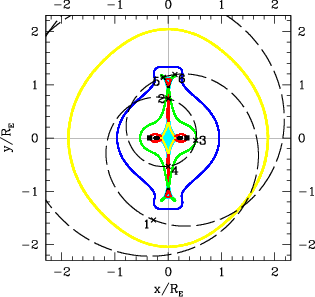
Figure 8: System 1. Panel (a) shows a lightcurve calculated for $b=0.5$. The magnification map for this binary is displayed in panel (b). The two black squares on the $y=0$ axis mark the location of the two stars. The path of the source star, moving clockwise in the binary reference frame, is drawn as a dashed black line. The numbered black crosses mark the locations along the trajectory which produce the strongest features in the lightcurve in panel (a). Note that rotation of the lens system produces three caustic crossings for a relatively large impact parameter event.

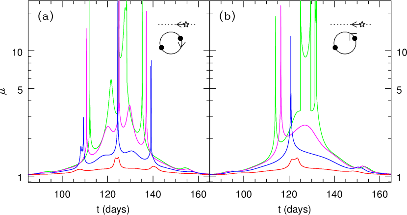
Figure 9: System 1: A sequence of microlensing lightcurves for System 1 calculated for $b=0.1,\,0.3,\,0.7,\,1.3$, in order of decreasing magnification. The two panels illustrate the difference between retrograde (panel a) and prograde (panel b) geometry, as illustrated Panel on the left shows the results for a binary rotating clockwise (retrograde), while the one on the right rotates counterclockwise (prograde).

Figure 8 illustrates the effect of binary rotation on a relatively high impact parameter microlensing lightcurve for System 1. Panel (b) shows the path of the source in the fixed frame of the binary. It appears to circle the binary center of mass clockwise, completing roughly two revolutions while the overall magnification remains above 1.05. The spiraling source path insures that a much larger portion of the lensing plane is seen by the source. As a result there are many more strong features in the resulting lightcurve than can be expected for a typical binary lightcurve for which rotation does not play a large role. The repetitive nature of these features suggests the effects of orbital motion, and the standard Lomb-Scargle analysis of the lightcurve does identify the signal as periodic (though the false signal probability is just over 2%, close to our threshold). The inferred period is 45 days, close to the actual value of 42 days.

Because it increases the fraction of the magnification plane explored in each lensing event, orbital rotation significantly increases our chances of detecting binarity for large impact parameter events. Figure 9  (a) shows a sequence of lightcurves for four different impact parameters. Even for a distant approach, $b=1.3$, there is a hint of a periodicity in the three magnification bumps apparent in the lightcurve. This sequence also underscores the need for relative motion correction in determining the period via the timing analysis. The periodicity is very apparent in all of the curves, but it appears that the underlying period appears different for each one.

A comparison between panels (a) and (b) in Figure 9 emphasize the importance of the direction of binary rotation with respect to the lens-source relative motion. The cartoons in the upper-right-hand corner in each panel illustrate our definitions of prograde and retrograde rotation; note that the binary center-of-mass is assumed to be fixed, while the source moves past the binary. The retrograde motion (panel a) corresponds to the case when the companion closest to the projected position of the source moves opposite to the direction of source velocity. In this situation, the effects of binary rotation are amplified and the lightcurves show more peaks on average. The opposite is true for prograde rotation (anel b), when the closest companion and the source move in the same direction, partially canceling the effects of rotation. As a result, the prograde lightcurves in panel (b) look more like the “standard” binary microlensing events than those in panel (a).

3.3.2 System 2

The specific lens system considered: A nearly solar-mass binary. System 2 can represent a common type of binary in which both stars are on the main sequence. The mass ratio we chose is similar to the value at the peak of the observed distribution of binary mass ratios measured by Duquennoy & Mayor (1982). The orbital separation is not unusual, although the observed distribution peaks at somewhat larger values.

Alternatively, System 2 represents a binary in which one or both components have already evolved. In fact the smaller mass ($0.3\,M_{\odot}$) and the orbital period ($44$ days) satisfy the period/core-mass relationship (Rappaport et al. 2005). This relationship applies to a situation in which a giant star filled its Roche lobe, transferring mass to a companion until the time at which the giant’s stellar envelope was depleted. In this case, the depletion of the envelope left behind a helium WD with a mass of $0.3\,M_{\odot}.$ There are two possibilities. This core could be the remnant of the star that was initially the most massive. In this case the $1.3\,M_{\odot}$ star is still on the main sequence. Since it would have gained mass from the giant’s envelope, it can be viewed as a “blue straggler”, with a larger mass than its initial mass. On the other hand, the core could be the remnant of the initially less-massive star. In this case the $1.3\,M_{\odot}$ star has already evolved and is either a WD or a NS. The compact object is also likely to have gained mass from the giant that evolved to become the $0.3\,M_{\odot}$ heium WD. If today’s more massive star is a WD, then its mass is close to the Chandrasekhar mass and it is a near-miss Type Ia supernova. If instead it is a neutron star, it may have been spun up by mass accretion and may therefore be a millisecond pulsar. Thus, this single example, one of many that could have been chosen, illustrates that important classes of evolved stellar binaries can imprint signatures of rotation onto lensing light curves.

The light curve: The left-hand pane; of Figure 10 shows two light curves generated by this lens; as before, the source is assumed to be located near the Galactic center. The timescale ratio is $\tau_{E}/P=6.4$, so the binary goes through many full rotations during the duration of the event. The resulting light curves have a highly periodic structure with the source returning over and over to roughly the same regions of the lens magnification plane. It is typical that the increasing numbers of features are associated with short orbital periods and small values of $\alpha$, so that the amplitude of the deviations is relatively small (see Figure 4). It is easy to understand this by noting that the timescale ratio depends inversely on $\alpha$ (see Eq. [5]). Indeed, for this system $\alpha=0.35$, which is half of its value for the brown dwarf binary we discussed in the previous section. Smaller $\alpha$ implies that, over long time scales, the binary lensing features are less prominent, so overall the lightcurves look more like those due to single-mass lenses.

Unsurprisingly, the Lomb-Scargle analysis for both of the lightcurves shown in Figure 10(a) extracts the orbital period with a discrepancy from the true orbital period smaller than $4\%$, with a very high degree of confidence. Since the timescale ratio is large, the corrections for the relative lens-source motion are not very important in this case.

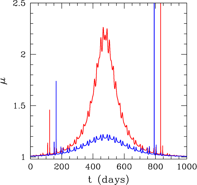
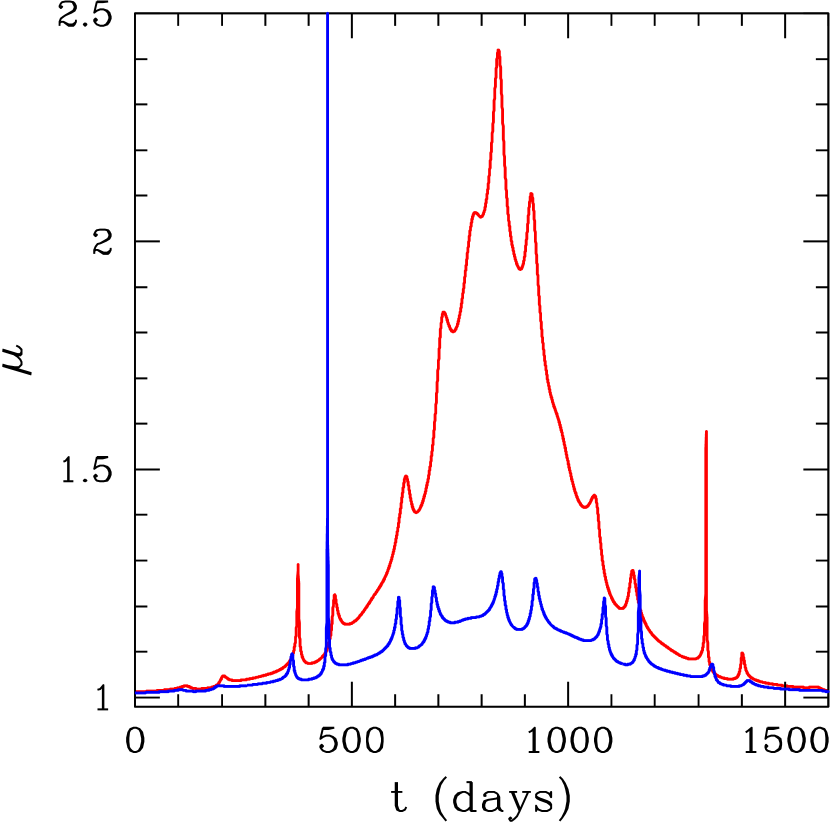
Figure 10: System 2 and System 4: Panel (a) shows a sequence of microlensing lightcurves for System 2 calculated for $b=0.5,\,1.3,\,2.0$, in order of decreasing magnification. Panel (b) shows lightcurves for System 4 corresponding to $b=0.5,\,1.3$.

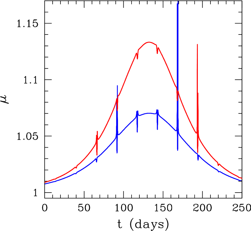
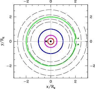
Figure 11: System 3: Panel (a) shows lightcurves for System 3, calculated for $b=1.5,\,2.0$. The magnification map for this binary in displayed in panel (b). The black curve is the path of the source in the binary frame which corresponds to the red lightcurve in panel (a). Only the inspiral part of the source path is shown for clarity.

3.3.3 System 3

The specific lens system considered: Jupiter Orbiting a Dwarf Star. Planets with masses comparable to or larger than that of Jupiter are common, and many orbit solar-mass stars with periods of days. (Di Stefano 2012) showed that orbital motion can be detectable. The maximum change in magnification from the point-lens form occurs when the distance between source and lens is equal to $1/\alpha-\alpha$. The position of the perturbation is a function of the orbital phase, providing a periodic signal when the Einstein crossing time is long enough. We consider a stellar mass of $0.8\,M_{\odot};$ the planet’s mass is $2\,M_{J},$ yielding $q=0.0025.$

The light curve: Figure 11  (a) shows two light curves for System 3. The distances of closest approach are $b=1.5$ and for $b=2$ for the upper and lower light curve, respectively. The light-curve deviations are regular but small in amplitude. A Lomb-Scargle test fails to pick up the orbital period in this case. This is mainly due to the low amplitude and small duration of the observed features (in the context of our adopted once-per-day lightcurve sampling with 1% photometry errors), as well as the oscillatory behavior of the magnification within the features. However, an observation with sufficiently high cadence and sensitivity would allow the period to be measured directly, since the timescale ratio ($\tau_{E}/P=3.6$) is large. Merely folding the lightcurves to match the sharp peaks yields the period of 26 days, very close to the true orbital period of 28 days for this system. Since the deviations in the isomagnification diagram are very asymmetric (due to the very low mass ratio for this system), we expect roughly one deviation per orbit, as opposed to two expected when $q$ is of order unity. So the factor of 2 correction we routinely apply in our period analysis is not appropriate here.

An interesting point to note is that this type of planet-induced deviation can be detected even when the distance of closest approach between the source and lens is large, and the peak source magnification is low. Figure 11(b) shows the source path relative to the lens system. The deviations from the point-lens form do indeed occur when the distance between source and lens is $1/\alpha-\alpha\sim 2.25$. The case of close-orbit planets is discussed in more detail in Di Stefano 2012.

3.3.4 System 4

The specific lens system considered: A High-Mass Binary. When the lens is a high-mass star, $\tau_{E}$ can be large because the associated value of $R_{E}$ is larger for any given $D_{L}.$ Furthermore, for a given value of the semimajor axis, the period is shorter. The overall effect can be to produce large values of $\tau_{E}/P_{orb}$. If the primary of such a lens is a main-sequence star, the light curve is likely to be affected by blending, making the detection more difficult unless the lensed source is also very bright. Nevertheless, some such events should be detectable.

Perhaps the case of greatest interest is that in which the most massive component is a black hole. If the primary star in System 4 is a BH, and if the secondary is on the main sequence, the evolution of the secondary will eventually cause it to donate mass to the BH, probably through winds in this case, making the system detectable as an X-ray binary. System 4 is 200 pc from the Sun, but exactly the same results would be obtained for an identical binary located at $D_{L}=7.8\,{\rm kpc}$.

The light curve: Two lightcurves for this system are shown in Figure 10(b). The periodicity is clearly evident in the data and is picked up by the Lomb-Scargle analysis with very high significance. However, the timescale ratio is low enough that the relative motion corrections become important. The inferred periods are 161 days and 230 days for $b=1.3$ and 0.5, respectively, significantly different from the true orbital period of the system. The long-lasting low magnification light curve could easily be mistaken for a variable star.

3.3.5 System 5

The specific lens system considered: binary planets. The class of free-floating planets may include binaries; these would be difficult or impossible to discover except through their action as gravitational lenses. For discovered systems close enough to us, direct imaging could be employed to verify the nature of the system. In addition, planets orbiting stars could have moons with masses in the range of planetary masses. Figure 2 shows lens masses that decrease from the bottom panel to the top panel. Extrapolating to even lower masses, i.e., to the planetary regime, we expect values of $\alpha$ close to $\sim\alpha=0.2$, implying small amplitude deviations from the point-mass form. For our System 5 we choose a fairly massive binary in which one companion is 6 times more massive than Jupiter while the mass of the other is 2 times larger that that of Saturn.

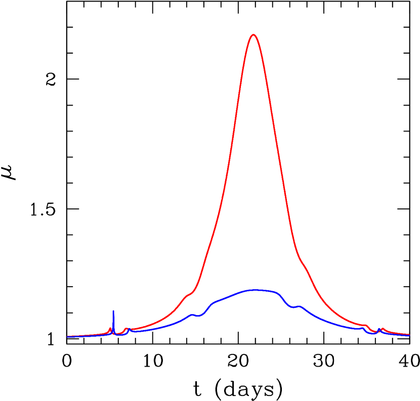
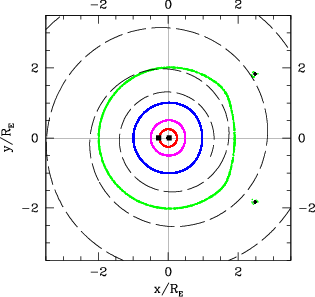
Figure 12: System 5: Panel (a) shows light curves for System 5, calculated for $b=0.5,\,1.3$. The magnification map for this binary in displayed in panel (b). The black curve shows the path of the source in the binary frame corresponding to the blue lightcurve in panel (a). Only the inspiral part of the path is shown for clarity.

The light curve: Figure 12  (a) shows two representative lightcurves for this binary, while the isomagnification diagram with the source path for the lightcurve with $b=1.3$ are displayed in panel (b). Note the similarity between the isomagnification contours for this system and System 3, though the mass ratio here is not as extreme, producing less asymmetry in the deviations from the point-lens form. As expected, the observed deviations are relatively small (a few percent), but unquestionably periodic with an apparent period of $\sim 10\,{\rm days}$. As was the case for System 3, Lomb-Scargle analysis does not pick up a believable period here, but one can easily be seen with improved photometric sensitivity. Again, as in System 3, low value of the mass ratio makes the interpretation of the result difficult, since correcting by a factor of 2 only confuses the matter. In addition, $\tau_{E}/P=1.4$ means that relative motion corrections are important.

4 Conclusion

We have shown that orbital motion produces significant phase shifts during gravitational lensing events for multiple lenses with wide ranges of parameters and distances from us. This seems to be an odd result, because phase changes during lensing events have needed to be invoked only a small number of times, and the changes have been relatively minor. The reason may be that many of the expected deviations are difficult to identify. Some light curves exhibiting rotational effects may be extreme enough that the event is not recognized as being due to lensing or else is difficult to fit. More often, the effects associated with orbital motion are subtle, and their discovery requires temporally dense, high-sensitivity sampling. Since different fields are monitored in different ways, only about $10\%$ of the events being discovered at present receive monitoring that is adequate for these purposes. The detection efficiency may be low for many types of events (Penny et al. 2011b).

There are, however, some events for which the orbital-motion-detection efficiency should be close to unity: events caused by short period lenses. For example, if a Neptune-mass or Jupiter-mass planet orbits a solar-mass star at $\sim 0.3\,R_{E},$ then even distances of closest approach as large as $2.5-3\,R_{E}$ could produce distinctive, almost-periodic deviations (Di Stefano 2012). These would occur during a stellar lens event that produces a peak magnification of only $\sim 1-3\%$. The signatures of the planet could be easily missed without a filter that tests for intervals of periodicity in otherwise stable light curves. With such a filter, however, detection of the signature is guaranteed for a wide range of mass ratios and with sampling as good as the present-day sampling already applied in several fields today (Di Stefano 2012). Thus, if $1/2$ of all stars have planets (a very conservative estimate), and if $1/2$ of these have nested planets, and if $1/2$ of these have planets with orbital separations between $0.25\,R_{E}$ and $0.5\,R_{E}$, and if the mass ratios are larger than $\sim 1/10^{5}$ in $1/4$ of these cases, then roughly $3\%$ of lensing events by stars would exhibit small signatures of the planet’s presence for approaches between $2\,R_{E}$ and $4\,R_{E}$; in many cases (depending on the relative velocities), the signatures will repeat.

A similar argument applies to binary systems, where orbital distributions are typically modeled as being uniform in logarithm over $8$ intervals. If $1/2$ of all stellar systems are binaries, and the $1/16$ of the stellar primaries have a companion in an orbit between $0.25\,R_{E}$ and $0.5\,R_{E}$, this also suggests that $3\%$ of all stellar systems would have a significant probability of exhibiting orbital motion during lensing events. Higher order multiples, which constitute $\sim 10\%$ of all stellar multiples are even more likely to have one companion in an orbit for which orbital motion can be detected.

If, therefore, signatures of orbital motion are detectable in only $10\%$ of events discovered today, we might expect $.006$ of the $2000$ events discovered per year to exhibit detectable evidence of orbital motion. This corresponds to $12$ events per year, half of them planet-lens events. In addition, orbital motion could be discovered in $42$ of the $\sim 14,000$ already-known events, $\sim 21$ of them associated with planet lenses. Even if lower estimates of the population (Penny et al. 2011a) apply, the numbers would still be significant, and will become more so with the advent of programs such as KMTNet. In addition, the excellent astrometric and photometric precision possible with space missions (GAIA, Kepler, TESS WFIRST) will make detailed studies of orbital motion a regular part of microlensing discoveries.

Finally, orbital motion will play an important role in the study of predicted gravitational lensing events. When the proper motion of a star within a few hundred parsecs has been measured, we can check whether it has a high probability of passing close enough to a background star to cause a lensing event (see, e.g., Lépine & Di Stefano 2012, Di Stefano et al. 2013). The equations in Section 2 show that the Einstein radii, $R_{E}$, of nearby stars tend to be small. Thus, if the orbital periods of planets orbiting these stars have a distribution similar to the distribution measured for the orbits of already-discovered exoplanets, we expect that, during lensing events, the orbital phase will shift significantly for close-orbit planets ($a<0.5\,R_{E}$), and often for planets in the “resonant” zone ($0.5\,R_{E}<a<2\,R_{E}$), and in some cases even for planets in wider orbits. Observing campaigns planned to monitor these predicted events will measure the masses of the central star and its planets, determine the orbital period(s), and provide constraints on the orbital inclination. For many of these systems, subsequent observations can verify the orbital properties and can be used to learn even more. Planetary systems studied during observing campaigns for predicted events will eventually become among the best studied exoplanetary systems.

Acknowledgements: It is a pleasure to acknowledge early contributions by Christopher Night and help from James Matthews and Xinyi Guo. This work was supported in part by support from NSF AST-1211843, AST-0708924 and AST-0908878 and NASA NNX12AE39G AR-13243.01-A.

References

- Albrow et al. (2000) Albrow, M. D. et al. 2000, ApJ, 534, 894
- An et al. (2002) An, J. H. et al. 2002, ApJ, 572, 521
- Borucki & Koch (2012) Borucki, W. J., & Koch, D. G. 2012, EGU General Assembly Conference Abstracts, 14, 6561
- Di Stefano et al. (2013) Di Stefano, R., Matthews, J., & Lépine, S. 2013, ApJ, 771, 79
- Di Stefano (2012) Di Stefano, R. 2012, ApJ, 752, 105
- Di Stefano (2008) Di Stefano, R. 2008, arXiv:0801.1511
- Di Stefano & Night (2008) Di Stefano, R., & Night, C. 2008, arXiv:0801.1510
- Dominik (1998) Dominik, M. 1998, A&A, 329, 361
- Dominik & Sahu (2000) Dominik, M., & Sahu, K. C. 2000, ApJ, 534, 213
- Dubath et al. (2007) Dubath, F., Alice Gasparini, M., & Durrer, R. 2007, Phys. Rev. D, 75, 024015
- Duquennoy & Mayor (1991) Duquennoy, A., & Mayor, M. 1991, A&A, 248, 485
- Gaudi et al. (2008) Gaudi, B. S., Bennett, D. P., Udalski, A., et al. 2008, Science, 319, 927
- Geissler et al. (2011) Geissler, K., Metchev, S., Kirkpatrick, D., Berriman, G. B., Looper, D. 2011, ArXiv Astrophysics e-prints, arXiv:1103.1160v1
- Guo et al. (2011) Guo, X., Esin, A., Di Stefano, R., & Taylor, J. 2011, arXiv:1112.4608
- Henderson et al. (2014) Henderson, C. B., Gaudi, B. S., Han, C., et al. 2014, ApJ, 794, 52
- Ioka et al. (1999) Ioka, K., Nishi, R., & Kan-Ya, Y. 1999, Progress of Theoretical Physics, 102, 983
- Jaroszynski (2002) Jaroszynski, M. 2002, Acta Astronomica, 52, 39
- Jaroszynski et al. (2006) Jaroszynski, M. et al. 2006, Acta Astronomica, 56, 307
- Kirkpatricket al. (2011) Kirkpatrick, J. D. et al. 2011, ArXiv Astrophysics e-prints, arXiv:1108.4677v1
- Lépine & DiStefano (2012) Lépine, S., & DiStefano, R. 2012, ApJ, 749, LL6
- Mao & Paczynski (1991) Mao, S. & Paczynski, B. 1991, ApJ, 374, L37
- McCaughrean et al. (2004) McCaughrean, M. J. et al. 2004, A&A, 413, 1029
- Moe & Di Stefano (2013) Moe, M., & Di Stefano, R. 2013, ApJ, 778, 95
- Moe & Di Stefano (2013) Moe, M., & Di Stefano, R. 2013, IAU Symposium, 281, 240
- Nelemans et al. (2013) Nelemans, G., Toonen, S., & Bours, M. 2013, IAU Symposium, 281, 225
- Park et al. (2013) Park, H., Udalski, A., Han, C., et al. 2013, ApJ, 778, 134
- Penny et al. (2011) Penny, M. T., Kerins, E., & Mao, S. 2011a, MNRAS, 417, 2216
- Penny et al. (2011) Penny, M. T., Mao, S., & Kerins, E. 2011b, MNRAS, 412, 607
- Prestwich et al. (2007) Prestwich, A. H., Kilgard, R., Crowther, P. A., et al. 2007, ApJ, 669, L21
- Proft et al. (2011) Proft, S., Demleitner, M., & Wambsganss, J. 2011, A&A, 536, AA50
- Rappaport et al. (1995) Rappaport, S., Podsiadlowski, P., Joss, P. C., Di Stefano, R., & Han, Z. 1995, MNRAS, 273, 731
- Ricker et al. (2014) Ricker, G. R., Winn, J. N., Vanderspek, R., et al. 2014, Proc. SPIE, 9143, 914320
- Scholtz et al. (2003) Scholtz, R.-D., McCaughrean, M. J., Lodieu, N., Kuhlbrodt, B. 2003, A&A, 398, 29
- Volk et al. (2003) Volk, K., Blum, R., Walker, G., & Puxley, P. 2003, IAUC 8188
- Yee et al. (2014) Yee, J. C., Albrow, M., Barry, R. K., et al. 2014, arXiv:1409.2759