Stationary electro-vacuum fields around black holes

Abstract

This is the second lecture of ‘RAGtime’ series on electrodynamical effects near black holes. We will summarize the basic equations of relativistic electrodynamics in terms of spin-coefficient (Newman-Penrose) formalism.

The aim of the lecture is to present important relations that hold for exact electro-vacuum solutions and to exhibit, in a pedagogical manner, some illustrative solutions and useful approximation approaches. First, we concentrate on weak electromagnetic fields and we illustrate their structure by constructing the magnetic and electric lines of force. Gravitational field of the black hole assumes axial symmetry, whereas the electromagnetic field may or may not share the same symmetry. With these solutions we can investigate the frame-dragging effects acting on electromagnetic fields near a rotating black hole. These fields develop magnetic null points and current sheets. Their structure suggests that magnetic reconnection takes place near the rotating black hole horizon. Finally, the last section will be devoted to the transition from test-field solution to exact solutions of coupled Einstein-Maxwell equations.

New effects emerge within the framework of exact solutions: the expulsion of the magnetic flux out of the black-hole horizon depends on the intensity of the imposed magnetic field.

1 Introduction

Electromagnetic fields play an important role in astrophysics. Near rotating compact bodies, such as neutron stars and black holes, the field lines are deformed by an interplay of rapidly moving plasma and strong gravitational fields. Here we will illustrate purely gravitational effects by exploring simplified vacuum solutions in which the influence of plasma is ignored but the presence of strong gravity is taken into account.

In the first lecture of this workshop series (Karas 2005, Paper I) we summarized the basic equations of relativistic magnetohydrodynamics (MHD). In that paper we employed standard tensorial notation and we focused our attention on situations when the plasma motion is governed by MHD and gravitational effects are competing with each other in the vicinity of a black hole. We limited our discussion to axially symmetric and stationary flows. The latter assumption will be still maintained in the present talk. In fact, we will restrict ourselves to purely electro-vacuum solution, however, we will discuss them in greater depth and, more importantly, we will employ the elegant formalism of null tetrads. We do not derive new solutions or technique in these lectures, instead, we summarise useful relations in the form of brief notes paying special attention to effects of strong gravity.

One new point is mentioned in conclusion: with exact solutions of Einstein-Maxwell electrovacuum fields, an aligned magnetic flux becomes expelled from a rotating black hole as an interplay between the shape of magnetic lines of force (which become pushed out of the horizon) and the concentration of the magnetic flux tube toward the rotation axis (which becomes more concentrated for strong magnetic fields because of their own gravitational effect). This is, however, important only for very strong magnetic fields only, where ‘very strong’ means that the magnetic field contributes to the space-time metric.

2 Definitions, notation, and basic relations

Field equations

We start with Einstein’s equations which, in the notation of Paper I, take a familiar form of a set of coupled partial differential equations (e.g. Chandrasekhar 1983),

$$R_{\mu\nu}-\textstyle{\frac{1}{2}}Rg_{\mu\nu}=8\pi T_{\mu\nu},$$ (1)

where the right-hand side source terms $T_{\mu\nu}$ are of purely electromagnetic origin,

$$T^{\alpha\beta}\equiv T^{\alpha\beta}_{\rm EMG}=\frac{1}{4\pi}\left(F^{\alpha\mu}F^{\beta}_{\mu}-\frac{1}{4}F^{\mu\nu}F_{\mu\nu}g^{\alpha\beta}\right),$$ (2)

$${T^{\mu\nu}}_{;\nu}=-F^{\mu\alpha}j_{\alpha},\qquad{F^{\mu\nu}}_{;\nu}=4\pi j^{\mu},\qquad{{}^{\star}F^{\mu\nu}}_{;\nu}=4\pi\mathcal{M}^{\mu}.$$ (3)

where ${}^{\star}F_{\mu\nu}\equiv\frac{1}{2}{\varepsilon_{\mu\nu}}^{\rho\sigma}F_{\rho\sigma}$. We assume that the electromagnetic test-fields reside in a curved background of a rotating black hole. Such solutions can be found by solving for the electromagnetic field in a fixed background geometry of Kerr metric (Thorne et al. 1986; Gal’tsov 1986). Here we study classical solutions for (magnetised) Kerr-Newman black holes that possess a horizon. Higher-dimensional black holes and black rings in external magnetic fields were explored by, e.g., Ortaggio (2005), Yazadjiev (2006), and references cited therein, whereas an extension to the case of naked singularity has been discussed recently by Adámek & Stuchlík (2013).

Killing vectors generate a test-field solution

The presence of Killing vectors corresponds to the symmetry of the spacetime (Chandrasekhar 1983; Wald 1984), such as stationarity and axial symmetry. Killing vectors satisfy the well-known equation,

$$\xi_{\mu;\nu}+\xi_{\nu;\mu}=0,$$ (4)

where coordinate system is selected in such a way that the following condition is satisfied: $\xi^{\mu}=\delta^{\mu}_{\rho}$. One can check that Killing vectors obey a sequence of relations:

$$0=\xi_{\mu;\nu}+\xi_{\nu;\mu}=\xi_{\mu,\nu}-\Gamma^{\lambda}_{\mu\nu}\xi_{\lambda}+\xi_{\nu,\mu}-\Gamma^{\lambda}_{\mu\nu}\xi_{\lambda}=g_{\mu\nu,\rho}.$$ (5)

The last equality (5) states that because of symmetry the metric tensor does not depend $x^{\rho}$ coordinate.

The electromagnetic field may or may not conform to the same symmetries as the gravitational field. Naturally, the problem is greatly simplified by assuming axial symmetry and stationarity for both fields. In a vacuum spacetime, Killing vectors generate a test-field solution of Maxwell equations. We define the electromagnetic field by associating it with the Killing vector field,

$$F_{\mu\nu}=2\xi_{\mu;\nu}.$$ (6)

Then

$$F_{\mu\nu}=2\xi_{\mu;\nu}=-2\xi_{\nu;\mu}=-F_{\nu\mu},$$ (7)

$$F_{\mu\nu}=\xi_{\mu;\nu}-\xi_{\nu;\mu}\equiv\xi_{[\mu;\nu]}.$$ (8)

By employing the Killing equation and the definition of Riemann tensor, i.e., the relations $\xi_{\mu;\nu;\sigma}-\xi_{\mu;\sigma;\nu}=-R_{\lambda\mu\nu\sigma}\xi^{\lambda}$, and $R_{\lambda[\mu\nu\sigma]\mathrm{cycl}}=0$, we find:

$$\xi_{\mu;\nu;\sigma}=R_{\lambda\sigma\mu\nu}\xi^{\lambda},\qquad{\xi^{\mu;\nu}}_{;\nu}={R^{\mu}}_{\lambda}\xi^{\lambda}.$$ (9)

The right-hand side vanishes in vacuum, hence

$${F^{\mu\nu}}_{;\nu}=0.$$ (10)

It follows that the well-known field invariants are given by relations

$$\mbox{\boldmath$E.B$}=\textstyle{\frac{1}{4}}\,{{}^{\star}}F_{\mu\nu}F^{\mu\nu},\qquad B^{2}-E^{2}=\textstyle{\frac{1}{2}}F_{\mu\nu}F^{\mu\nu}.$$ (11)

Magnetic and electric charges

We start from the axial and temporal Killing vectors, existence of which is guaranteed in any axially symmetric and stationary spacetime,

$$\xi^{\mu}=\frac{\partial}{\partial t},\qquad\tilde{\xi}^{\mu}=\frac{\partial}{\partial\phi}.$$ (12)

In the language of differential forms (e.g. Wald 1984),

$$\underbrace{\textstyle{\frac{1}{2}}F_{\mu\nu}{\,\rm d}x^{\mu}\wedge{\,\rm d}x^{\nu}}_{\mbox{${\bf F}$}}=\underbrace{\xi_{\mu,\nu}{\,\rm d}x^{\mu}\wedge{\,\rm d}x^{\nu}}_{\mbox{${\bf d}${\boldmath$\xi$}}}.$$ (13)

The above-given equations allow us to introduce the magnetic and electric charges in the form of integral relations,

$$\mbox{Magnetic\leavevmode\nobreak\ charge:\leavevmode\nobreak\ }\qquad 4\pi\mathcal{M}=\int_{\mathcal{S}}{\bf F} = \int_{\mathcal{S}}\mbox{${\bf d}${\boldmath$\xi$}}=0.$$ (14)

$$\mbox{Electric\leavevmode\nobreak\ charge:}\qquad 4\pi Q=\int_{\mathcal{S}}\mbox{\boldmath${}^{\star}F$} = \int_{\mathcal{S}}\mbox{{\boldmath${}^{\star}$}${\bf d}${\boldmath$\xi$}}=-8\pi M,$$ (15)

$$= \int_{\mathcal{S}}\mbox{{\boldmath${}^{\star}$}${\bf d}${\boldmath$\tilde{\xi}$}}=16\pi J,$$ (16)

where $M$ has a meaning of mass and $J$ is angular momentum of the source. Here, integration is supposed to be carried out far from the source, i.e. in spatial infinity of Kerr metric in our case. For example for the electric charge we obtain

$$4\pi Q=\int_{\mathcal{S}}\mbox{\boldmath${}^{\star}F$}=\int_{\mathcal{S}}\,^{\star}F_{\mu\nu}{\,\rm d}\sigma^{\mu\nu}=\int_{\mathcal{V}}2{F^{\tau\alpha}}_{;\alpha}{\,\rm d}\mathcal{V},$$ (17)

where ${\,\rm d}\sigma^{\mu\nu}={\,\rm d}_{1}x^{\mu}\wedge{\,\rm d}_{2}x^{\nu}={\,\rm d}\theta\,{\,\rm d}\phi$.

Wald’s field

In an asymptotically flat spacetime, $\partial_{\phi}$ generates uniform magnetic field, whereas the field vanishes asymptotically for $\partial_{t}$. These two solutions are known as the Wald’s field (Wald 1974; King et al. 1975; Bičák & Dvořák 1980; Nathanail & Contopoulos 2014):

$$F=\textstyle{\frac{1}{2}}B_{0}\left({\,\rm d}\tilde{\xi}+\frac{2J}{M}{\,\rm d}\xi\right).$$ (18)

Magnetic flux surfaces:

$$4\pi\Phi_{\mathcal{M}}=\int_{\mathcal{S}}\mbox{\boldmath$F$}\;=\;\mbox{const}.$$ (19)

Magnetic and electric Lorentz force are then given by equations

$$m\mbox{\boldmath$\dot{u}$}=q_{\rm{m}}\mbox{\boldmath${{}^{\star}}F.u$},\qquad m\mbox{\boldmath$\dot{u}$}=q_{\rm{e}}\mbox{\boldmath$F.u$}.$$ (20)

Finally, magnetic field lines (in the axisymmetric case):

$$\frac{{{\,\rm d}{r}}}{{{\,\rm d}\theta}}=\frac{B_{r}}{B_{\theta}},$$ (21)

Magnetic field lines lie in surfaces of constant magnetic flux (see below).

3 Spin-coefficient formalism of null tetrads for electromagnetic fields

The spin-coefficient formalism (Newman & Penrose 1962) is a special case of the tetrad formalism where tensors are projected onto a complete vector basis at each point in spacetime, The vector basis is chosen as a complex null tetrad, $l^{\mu}$, $n^{\mu}$, $m^{\mu}$, $\bar{m}^{\mu}$, satisfying conditions

$$l_{\nu}n^{\nu}=1,\qquad m_{\nu}\bar{m}^{\nu}=-1,$$ (22)

and zero all other combinations. A natural correspondence with an orthonormal tetrad reads

$$e_{(0)}=\frac{l+n}{\sqrt{2}},\quad e_{(1)}=\frac{l-n}{\sqrt{2}},\quad e_{(2)}=\frac{m+\bar{m}}{\sqrt{2}},\quad e_{(3)}=\frac{m-\bar{m}}{\Im\,\sqrt{2}}.$$ (23)

Null tetrads are not unambiguous, as the following three transformations maintain the tetrad properties:

(i)

$l\rightarrow l$, $m\rightarrow m+al$, $n\rightarrow n+a\bar{m}+\bar{a}m+a\bar{a}l$;

(ii)

$n\rightarrow n$, $m\rightarrow m+bm$, $l\rightarrow l+b\bar{m}+\bar{b}m+b\bar{b}n$;

(iii)

$l\rightarrow\zeta l$, $n\rightarrow\zeta^{-1}l$, $m\rightarrow e^{\Im\psi}m$;

with $\zeta$, $\psi\in\Re$.

Instead of six real components of $F_{\mu\nu}$, the framework of the null tetrad formalism describes the electromagnetic field by three independent complex quantities,

$$\Phi_{0} = F_{\mu\nu}l^{\mu}m^{\nu},$$ (24)

$$\Phi_{1} = \textstyle{\frac{1}{2}}F_{\mu\nu}\left(l^{\mu}n^{\nu}+\bar{m}^{\mu}m^{\nu}\right),$$ (25)

$$\Phi_{2} = F_{\mu\nu}\bar{m}^{\mu}n^{\nu}.$$ (26)

It can be checked that the backward transformation has a form

$$F_{\mu\nu}=\Phi_{1}\left(n_{[\mu}l_{\nu]}+m_{[\mu}\bar{m}_{\nu]}\right)+\Phi_{2}l_{[\mu}m_{\nu]}+\Phi_{0}\bar{m}_{[\mu}n_{\nu]}+c.c.$$ (27)

The Newman-Penrose formalism defines the following differential operators:

$$D\equiv l^{\mu}\partial_{\mu},\quad\delta\equiv m^{\mu}\partial_{\mu},\quad\bar{\delta}\equiv\bar{m}^{\mu}\partial_{\mu},\quad\Delta\equiv n^{\mu}\partial_{\mu}.$$ (28)

Furthermore, one introduces a set of spin coefficients (Ricci rotations symbols),

$$\alpha = -\textstyle{\frac{1}{2}}\left(n_{\mu;\nu}l^{\mu}\bar{m}^{\nu}-\bar{m}_{\mu;\nu}m^{\mu}\bar{m}^{\nu}\right),$$ (29)

$$\beta = \textstyle{\frac{1}{2}}\left(l_{\mu;\nu}n^{\mu}m^{\nu}-m_{\mu;\nu}\bar{m}^{\mu}m^{\nu}\right),$$ (30)

$$\gamma = -\textstyle{\frac{1}{2}}\left(n_{\mu;\nu}l^{\mu}n^{\nu}-\bar{m}_{\mu;\nu}m^{\mu}m^{\nu}\right),$$ (31)

$$\epsilon = \textstyle{\frac{1}{2}}\left(l_{\mu;\nu}n^{\mu}l^{\nu}-m_{\mu;\nu}\bar{m}^{\mu}l^{\nu}\right),$$ (32)

$$\kappa = l_{\mu;\nu}m^{\mu}l^{\nu},\qquad\leavevmode\nobreak\ \leavevmode\nobreak\ \lambda=-n_{\mu;\nu}\bar{m}^{\mu}\bar{m}^{\nu},$$ (33)

$$\rho = l_{\mu;\nu}m^{\mu}\bar{m}^{\nu},\qquad\mu=-n_{\mu;\nu}\bar{m}^{\mu}m^{\nu},$$ (34)

$$\sigma = l_{\mu;\nu}m^{\mu}m^{\nu},\qquad\nu=-n_{\mu;\nu}\bar{m}^{\mu}n^{\nu},$$ (35)

$$\tau = l_{\mu;\nu}m^{\mu}n^{\nu},\qquad\leavevmode\nobreak\ \pi=-n_{\mu;\nu}\bar{m}^{\mu}l^{\nu}.$$ (36)

Despite a seemingly large number of variables we will find this notation very useful and practical later on. However, first it will be useful to give an explicit example.

Example of the null tetrad for Schwarzschild metric

The metric is written in the form

$${\,\rm d}s^{2}=\left(1-\frac{2M}{r}\right){\,\rm d}t^{2}-\left(1-\frac{2M}{r}\right)^{-1}{\,\rm d}r^{2}-r^{2}{\,\rm d}\theta^{2}-r^{2}\sin^{2}\theta{\,\rm d}\phi^{2}.$$ (37)

The appropriate null tetrad is then given by

$$l^{\mu} = \left([1-2M/r]^{-1},1,0,0\right),$$ (38)

$$n^{\mu} = \left(\textstyle{\frac{1}{2}},\textstyle{\frac{1}{2}}[1-2M/r],0,0\right),$$ (39)

$$m^{\mu} = \frac{1}{\sqrt{2}\,r}\left(0,0,1,\Im\sin^{-1}\theta\right).$$ (40)

An arbitrary type-D spacetime (e.g. the Schwarszchild metric) allows to set $\kappa=\sigma=\nu=\lambda=0$. In particular, for the Schwarzschild metric the explicit form of non-vanishing spin coefficients is:

$$\rho=-\frac{1}{r},\quad\mu=-\frac{1}{2r}\frac{1}{1-2M/r},\quad\alpha=-\beta=-\sqrt{2}\,r\cot\frac{\theta}{2},\quad\gamma=\frac{M}{2r^{2}}.$$ (41)

Maxwell’s equations

Maxwell’s equations adopt the form

$$(D-2\rho+2\epsilon)\Phi_{1}-(\bar{\delta}+\pi-2\alpha)\Phi_{0} = 2\pi J_{l},$$ (42)

$$(\delta-2\tau)\Phi_{1}-(\Delta+\mu-2\gamma)\Phi_{0} = 2\pi J_{m},$$ (43)

$$(D-\rho+2\epsilon)\Phi_{2}-(\bar{\delta}+2\pi)\Phi_{1} = 2\pi J_{\bar{m}},$$ (44)

$$(\delta-\tau+2\beta)\Phi_{2}-(\Delta+2\mu)\Phi_{1} = 2\pi J_{n}$$ (45)

with

$$J_{l} = l_{\mu}(j^{\mu}+\Im\mathcal{M}^{\mu}),$$ (46)

$$J_{m} = m_{\mu}(j^{\mu}+\Im\mathcal{M}^{\mu}),$$ (47)

$$J_{\bar{m}} = \bar{m}_{\mu}(j^{\mu}+\Im\mathcal{M}^{\mu}),$$ (48)

$$J_{n} = n_{\mu}(j^{\mu}+\Im\mathcal{M}^{\mu}).$$ (49)

These are four equations for three complex variables.

Teukolsky’s equations

Teukolsky (1973) derived the following form of Maxwell equations:

$$\Big{[}(D \!\!-\!\! \epsilon+\bar{\epsilon}-2\rho-\bar{\rho})(\Delta+\mu-2\gamma)$$ (50)

$$-(\delta-\beta-\bar{\alpha}-2\tau+\bar{\pi})(\bar{\delta}+\pi-2\alpha\Big{]}\Phi_{0}=2\pi J_{0},$$

$$\Big{[}(D \!\!+\!\! \epsilon+\bar{\epsilon}-\rho-\bar{\rho})(\Delta+2\mu)$$ (51)

$$-(\delta+\beta-\bar{\alpha}-\tau+\bar{\pi})(\bar{\delta}+2\pi\Big{]}\Phi_{1}=2\pi J_{1},$$

$$\Big{[}(\Delta \!\!+\!\! \gamma-\bar{\gamma}+2\mu+\bar{\mu})(D-\rho+2\epsilon)$$ (52)

$$-(\bar{\delta}+\alpha+\bar{\beta}-\bar{\tau}+2\pi)(\delta-\tau+2\beta\Big{]}\Phi_{2}=2\pi J_{2}$$

with

$$J_{0} = (\delta-\beta-\bar{\alpha}-2\tau+\bar{\pi})J_{l}-(D-\epsilon+\bar{\epsilon}-2\rho-\bar{\rho})J_{m},$$ (53)

$$J_{1} = (\delta+\beta-\bar{\alpha}-\tau+\bar{\pi})J_{\bar{m}}-(D+\epsilon+\bar{\epsilon}-\rho-\bar{\rho})J_{n},$$ (54)

$$J_{2} = (\Delta+\gamma-\bar{\gamma}+2\mu+\bar{\mu})J_{\bar{m}}-(\bar{\delta}+\alpha+\bar{\beta}+2\pi-\bar{\tau})J_{n}.$$ (55)

Clearly this is an extremely useful form: noticed that the above-given differential equations are entirely decoupled.

Example – Maxwell’s equations in Schwarzschild metric

$$\left[\frac{\partial}{\partial r}+\frac{2}{r}\right]\Phi_{1}+\frac{1}{\sqrt{2}r}{{}^{\star}}\bar{\partial}\Phi_{0} = 2\pi J_{l},$$ (56)

$$-\frac{1}{\sqrt{2}r}{{}^{\star}}{\partial}\Phi_{1}+\frac{1}{2}\left[\left(1-\frac{2M}{r}\right)\frac{\partial}{\partial r}+\frac{1}{r}\right]\Phi_{0} = 2\pi J_{m},$$ (57)

$$\left[\frac{\partial}{\partial r}+\frac{1}{r}\right]\Phi_{2}+\frac{1}{\sqrt{2}r}{{}^{\star}}\bar{\partial}\Phi_{1} = 2\pi J_{\bar{m}},$$ (58)

$$-\frac{1}{\sqrt{2}r}{{}^{\star}}{\partial}\Phi_{2}+\frac{1}{2}\left(1-\frac{2M}{r}\right)\left[\frac{\partial}{\partial r}+\frac{2}{r}\right]\Phi_{1} = 2\pi J_{n},$$ (59)

where the “edth” operator acts on a spin weight $s$ quantity $\eta$ is the following manner:

$${}^{\star}\partial\eta=-\left\{\sin^{s}\theta\left[\frac{\partial}{\partial\theta}+\frac{\Im}{\sin\theta}\frac{\partial}{\partial\phi}\right]\sin^{-s}\theta\right\}\eta.$$ (60)

Spin weight is defined by by the transformation property $\eta\rightarrow e^{\Im s\psi}\eta$ under the transformation $m\rightarrow e^{\Im\psi}m$. $\Phi_{0}$, $\Phi_{1}$, $\Phi_{2}$ have spin weights $s=1$, $0$, $-1$, respectively.

Spin harmonics

Spin harmonics form a complete set of orthonormal functions

$${}_{s}Y_{lm}(\theta,\phi)=\left\{\begin{array}[]{ll}\sqrt{\frac{(l-s)!}{(l+s)!}}\,^{\star}\partial^{s}Y_{lm}(\theta,\phi)&\mbox{\leavevmode\nobreak\ for\leavevmode\nobreak\ }0\leq s\leq l,\\ (-1)^{s}\sqrt{\frac{(l+s)!}{(l-s)!}}\,^{\star}\partial^{-s}Y_{lm}(\theta,\phi)&\mbox{\leavevmode\nobreak\ for\leavevmode\nobreak\ }-l\leq s\leq 0\end{array}\right.$$ (61)

with the orthogonality relation

$${\int_{0}^{2\pi}\int_{0}^{\pi}}{\leavevmode\nobreak\ {}_{s}}Y_{lm}(\theta,\phi)\;_{s}Y_{l^{\prime}m^{\prime}}(\theta,\phi)\,\sin\theta{\,\rm d}\theta{\,\rm d}\phi=\delta_{ll^{\prime}}\delta_{mm^{\prime}}.$$ (62)

A general stationary vacuum electromagnetic test field can be expanded in terms of spin-$s$ spherical harmonics.

3.1 Test fields in Schwarzschild spacetime

Bičák & Dvořák (1980) use the following expansion:

$$\Phi_{0} = {\sum_{l=1}^{\infty}}{\sum_{m=-l}^{l}}{{}^{0}}R_{lm}(r)\,_{1}Y_{lm}(\theta,\phi),$$ (63)

$$\Phi_{1} = {\sum_{l=0}^{\infty}}{\sum_{m=-l}^{l}}{{}^{1}}R_{lm}(r)\,_{0}Y_{lm}(\theta,\phi),$$ (64)

$$\Phi_{2} = {\sum_{l=1}^{\infty}}{\sum_{m=-l}^{l}}{{}^{2}}R_{lm}(r)\,_{-1}Y_{lm}(\theta,\phi).$$ (65)

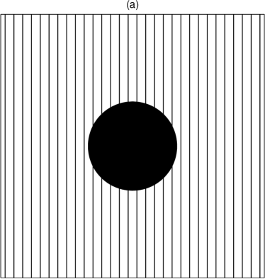
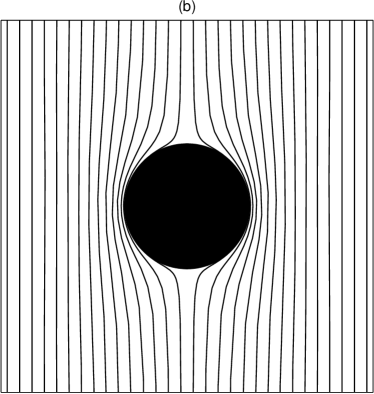
Figure 1: An axisymmetric case: (a) $a=0$ (static black hole), and (b) $a=M$ (maximally rotating black hole).

Then the equations for radial functions take a form

$$r(r-2M)\,^{0}R_{lm}^{\prime\prime}+4(r-M)\,^{0}R_{lm}^{\prime}-(l-1)(l+2)\,^{0}R_{lm} \!=\! -4\pi\,^{0}J_{lm},$$ (66)

$$r(r-2M)\,^{1}R_{lm}^{\prime\prime}+2(2r-3M)\,^{1}R_{lm}^{\prime}-(l-1)(l+2)\,^{1}R_{lm} \!=\! -4\pi\,^{1}J_{lm},$$ (67)

$$r(r-2M)\,^{2}R_{lm}^{\prime\prime}+4(r-2M)\,^{2}R_{lm}^{\prime}\leavevmode\nobreak\ \leavevmode\nobreak\ \leavevmode\nobreak\ \leavevmode\nobreak\ \leavevmode\nobreak\ \leavevmode\nobreak\ \leavevmode\nobreak\ \leavevmode\nobreak\ \leavevmode\nobreak\ \leavevmode\nobreak\ \leavevmode\nobreak\ \leavevmode\nobreak\ \leavevmode\nobreak\ \leavevmode\nobreak\ \leavevmode\nobreak\ \leavevmode\nobreak\ \leavevmode\nobreak\ \leavevmode\nobreak\ \leavevmode\nobreak\ \leavevmode\nobreak\ \leavevmode\nobreak\ \leavevmode\nobreak\ \leavevmode\nobreak\ \leavevmode\nobreak\ \leavevmode\nobreak\ \leavevmode\nobreak\ \leavevmode\nobreak\ \leavevmode\nobreak\ \leavevmode\nobreak\$$ (68)

$$-[(l-1)(l+2)+4M/r]\,^{2}R_{lm} \!=\! -4\pi\,^{2}J_{lm},$$ (69)

where

$${}^{0}J_{lm}(r) = \int J_{0}(r,\theta,\phi)\,_{1}\bar{Y}_{lm}(\theta,\phi)\,r^{2}{\,\rm d}\Omega,$$ (70)

$${}^{1}J_{lm}(r) = \int J_{1}(r,\theta,\phi)\,_{0}\bar{Y}_{lm}(\theta,\phi)\,r^{2}{\,\rm d}\Omega,$$ (71)

$${}^{2}J_{lm}(r) = \int J_{2}(r,\theta,\phi)\,_{-1}\bar{Y}_{lm}(\theta,\phi)\,r^{2}{\,\rm d}\Omega.$$ (72)

A vacuum field solution is given by a Fuchsian-type equation (Bičák & Dvořák 1980)

$$x(x-1)\frac{{\,\rm d}^{2}\,{}^{1}R_{lm}}{{\,\rm d}x^{2}}+(4x-3)\frac{{\,\rm d}\,^{1}R_{lm}}{{\,\rm d}x}-(l-1)(l+2)\,^{1}R_{lm}=0,$$ (73)

with $x\equiv r/(2M)$.

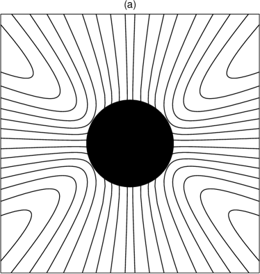
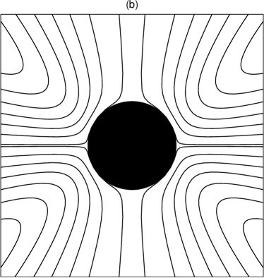
Figure 2: The case of (a) uniform aligned magnetic field near a fast rotating black hole ($a=0.95M$); (b) near the maximally rotating hole ($a=M$).

Two independent solutions can be found:

$$\left.\begin{array}[]{ll}^{1}R^{(I)}_{l}&=F(1-l,l+2,3;x),\\ ^{1}R^{(II)}_{l}&=\left(-x\right)^{-l-2}F(l,l+2,2l+2;x^{-1})\end{array}\right\}\quad\mbox{for\leavevmode\nobreak\ }l\neq 0,$$ (76)

$$\left.\begin{array}[]{ll}^{1}R^{(I)}_{0}&=\frac{1}{x^{2}}\ln(x-1)+\frac{1}{x}\\ ^{1}R^{(II)}_{0}&=\frac{1}{x^{2}}\end{array}\right\}\quad\mbox{for\leavevmode\nobreak\ }l=0.$$ (79)

A general solution reads ${}^{1}R_{lm}=a_{lm}\,^{1}R^{(I)}_{l}+b_{lm}\,^{1}R^{(II)}_{l}$, $a_{lm},\,b_{lm}=\mbox{const.}$ Inserting the solution for ${}^{1}R_{lm}$ in Maxwell equations Bičák & Dvořák (1980) find

$${}^{0}R_{lm} = a_{lm}\,^{0}R^{(I)}_{l}+b_{lm}\,^{0}R^{(II)}_{l}\;=\;\sqrt{\frac{2}{l(l+1)}}\frac{1}{r}\frac{{\,\rm d}}{{\,\rm d}r}\left(r^{2}\,{}^{1}R_{lm}\right),$$ (80)

$${}^{2}R_{lm} = a_{lm}\,^{2}R^{(I)}_{l}+b_{lm}\,^{2}R^{(II)}_{l},$$ (81)

where

$${}^{0}R^{(I)}_{l}=\frac{2\sqrt{2}}{\sqrt{l(l+1)}}\,F(1-l,l+2,2;x),$$ (82)

$${}^{0}R^{(II)}_{l}=-\sqrt{\frac{2l}{l+1}}\,(-x)^{-l-2}F(l+1,l+2,2l+2;x^{-1}),$$ (83)

$${}^{2}R^{(I)}_{l}=-\sqrt{\frac{2}{l(l+1)}}\,x^{-1}F(-l,l+1,2;x),$$ (84)

$${}^{2}R^{(II)}_{l}=-\sqrt{\frac{l}{2(l+1)}}\,(-x)^{-l-2}F(l+1,l,2l+2;x^{-1}).$$ (85)

We can select a physically appropriate solution by assuming a source between $r_{1}$ and $r_{2}$ ($r_{+}\leq r_{1}\leq r_{2}\leq\infty$). By seeking a well-behaved solution on horizon that vanishes at infinity, we find

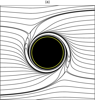
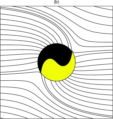
Figure 3: Equatorial plane is shown as viewed from top, i.e. along rotation axis, (a) in the frame of zero angular momentum observers orbiting at constant radius; (b) in the frame of freely falling observers. In the panel (b), two regions of ingoing/outgoing lines are distinguished by different levels of shading of the horizon. The hole rotates counter-clockwise ($a=M$). Based on Karas (1989), Dovčiak et al. (2000).

$$\left.\begin{array}[]{ll}\Phi_{0}&=\sum_{l,m}a_{l,m}\,^{0}R^{(I)}_{l}\,{}_{1}Y_{lm}\\ \Phi_{1}&=\sum_{l,m}a_{l,m}\,^{1}R^{(I)}_{l}\,{}_{0}Y_{lm}+\frac{E_{\rm a}}{r^{2}}\,_{0}Y_{00}\\ \Phi_{2}&=\sum_{l,m}a_{l,m}\,^{2}R^{(I)}_{l}\,{}_{-1}Y_{lm}\end{array}\right\}\quad\mbox{for\leavevmode\nobreak\ }2M\leq r<r_{1},$$ (89)

$$\left.\begin{array}[]{ll}\Phi_{0}&=\sum_{l,m}b_{l,m}\,^{0}R^{(II)}_{l}\,{}_{1}Y_{lm}\\ \Phi_{1}&=\sum_{l,m}b_{l,m}\,^{1}R^{(II)}_{l}\,{}_{0}Y_{lm}+\frac{E_{\rm b}}{r^{2}}\,_{0}Y_{00}\\ \Phi_{2}&=\sum_{l,m}b_{l,m}\,^{2}R^{(II)}_{l}\,{}_{-1}Y_{lm}\end{array}\right\}\quad\mbox{for\leavevmode\nobreak\ }r>r_{2}.\mbox{\leavevmode\nobreak\ \leavevmode\nobreak\ \leavevmode\nobreak\ \leavevmode\nobreak\ \leavevmode\nobreak\ \leavevmode\nobreak\ \leavevmode\nobreak\ \leavevmode\nobreak\ }$$ (93)

Two examples

First, a spherically symmetric electric field. A unique solution that is well-behaving both at $r=r_{+}$ and at $r\rightarrow\infty$: ${}^{1}R^{(II)}_{0}$. This term describes a weakly charged Reissner-Nordström black hole.

Second, an asymptotically uniform magnetic field:

$$F_{\mu\nu} \rightarrow B_{0}\mbox{\boldmath$e_{z}$}+B_{1}\mbox{\boldmath$e_{x}$},$$ (94)

i.e. $$F_{r\theta}\rightarrow-B_{1}\,r\sin\phi,$$ (97)

$$F_{r\phi}\rightarrow B_{0}\,r\,\sin^{2}\theta-B_{1}\,r\,\sin\theta\,\cos\theta\,\cos\phi,$$

$$F_{\theta\phi}\rightarrow B_{0}\,r^{2}\,\sin\theta\cos\theta+B_{1}\,r^{2}\,\sin^{2}\theta\,\cos\phi.$$

3.2 Magnetic and electric lines of force near a rotating black hole

Lorentz force acts on electric/magnetic monopoles residing at rest with respect to a locally non-rotating frame,

$$\frac{{\,\rm d}u^{\mu}}{{\,\rm d}\tau}\propto\,^{\star}\!F^{\mu}_{\nu}\,u^{\nu},\qquad\frac{{\,\rm d}u^{\mu}}{{\,\rm d}\tau}\propto F^{\mu}_{\nu}\,u^{\nu}.$$ (98)

Magnetic lines are defined (Christodoulou & Rufini 1973):

$$\frac{{\,\rm d}r}{{\,\rm d}\theta}=-\frac{F_{\theta\phi}}{F_{r\phi}},\qquad\frac{{\,\rm d}r}{{\,\rm d}\phi}=\frac{F_{\theta\phi}}{F_{r\theta}}.$$ (99)

In an axially symmetric case the magnetic flux is:

$$\Phi_{\rm m}=\pi B_{0}\left[r^{2}-2Mr+a^{2}+\frac{2Mr}{r^{2}+a^{2}\,\cos^{2}\!\theta}\left(r^{2}-a^{2}\right)\right]\sin^{2}\!\theta=\mbox{const}.$$ (100)

Notice: $\Phi_{\rm m}=0$ for $r=r_{+}$ and $a=M$. The flux is expelled out of the horizon (Meissner effect; Bičák & Ledvinka 2000; Penna 2014).

The electric fluxes and field lines can be introduced in a similar manner, one only needs to interchange the electromagnetic field tensor by its dual, the magnetic charge by the electric charge, and vice versa wherever they appear in the above-given formulae. It should be evident that the induced electric field vanishes in the non-rotating case. Based on the classical analogy with a rotating sphere, one would perhaps expect a quadrupole-type component, but here the leading term of the electric field arises due to gravomagnetic interaction which is a purely general-relativistic effect, and this electric field falls off radially as $r^{-2}$.

Magnetic field lines reside in surfaces of constant magnetic flux, and this way the lines of force are defined in an invariant way (see Fig. 1). Electric field is induced by the gravito-magnetic influence of the black hole. The resulting field lines are shown in Fig. 2. An asymptotic form of the electric field-lines reads

$$\frac{{\,\rm d}r}{{\,\rm d}\lambda} = \frac{B_{0}aM}{r^{2}}\left(3\cos^{2}\theta-1\right)\;+\;\frac{3B_{\perp}aM}{r^{2}}\,\sin\theta\,\cos\theta\,\cos\phi+\mathcal{O}\left(r^{-3}\right),$$ (101)

$$\frac{{\,\rm d}\theta}{{\,\rm d}\lambda} = \mathcal{O}\left(B_{\perp}r^{-3}\right),\qquad\frac{{\,\rm d}\phi}{{\,\rm d}\lambda}\;=\;\mathcal{O}\left(B_{\perp}r^{-3}\right).$$ (102)

As mentioned above, an aligned magnetic field produces an asymptotically radial electric field, rather than a quadrupole field, expected under these circumstances in the classical electrodynamics. This difference is due to rotation of the black hole.

Fig. 3 shows the structure of a uniform magnetic field perpendicular to the black hole rotation axis (Bičák & Karas 1989; Karas et al. 2009, 2012, 2013, 2014). We notice the enormous effect of frame-dragging which acts on field lines and distorts them in the sense of black hole rotation. Nevertheless, some field lines still enter the horizon and bring the magnetic flux into the black hole (naturally, the same magnetic flux has to emerge out of the horizon, so that the total flux through the black hole vanishes and its magnetic charge is equal zero).

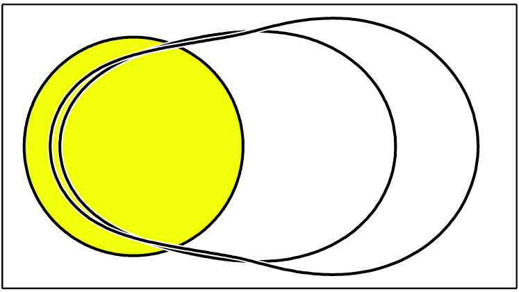
Figure 4: Cross-sectional area for the capture of magnetic flux by a rotating black hole. The three curves correspond to different values of the black-hole angular momentum: $a=0$ (cross-section is the circle; its projection coincides with the black-hole horizon, indicated by yellow colour), $a=0.95\,M$, and $a=M$. The enclosed area contains the field lines of the asymptotically perpendicular magnetic field whiech eventually enter into the black hole horizon. From the graph we notice that this area grows with the black hole spin and its shape is distorted by the gravitomagnetic interaction.

We notice that magnetic null points emerge near the black hole, suggesting that magnetic reconnection can be initiated by the purely gravitomagnetic effect of the rotating black hole. Indeed, this new reconnection mechanism has been only recently proposed (Karas & Kopáček 2009) in the context of particle acceleration processes near magnetized black holes. The capture of magnetic field lines is further illustrated in Fig. 4 where we plot the black hole effective cross sectional area.

Surface charge on the horizon

Surface charge is formally defined by the radial component of electric field in non-singular coordinates (Thorne et al. 1986),

$$\sigma_{\mathrm{H}} = \frac{B_{0}a}{4\pi\Sigma_{+}}\left[r_{+}\sin^{2}\theta-\frac{M}{\Sigma_{+}}\left(r_{+}^{2}-a^{2}\cos^{2}\theta\right)\left(1+\cos^{2}\theta\right)\right]$$ (104)

$$+\frac{B_{\perp}a}{4\pi\Sigma_{+}}\,\sin\theta\,\cos\theta\left[\frac{Mr_{+}}{\Sigma_{+}}+1\right]\left[a\sin\psi-r_{+}\cos\psi\right],$$

with

$$\psi=\phi+\frac{a}{r_{+}-r_{-}}\,\ln\frac{r-r_{+}}{r-r_{-}}\,\propto\ln(r-r_{+}).$$ (105)

For $a\ll M$,

$$\sigma_{\mathrm{H}}=\frac{a}{16\pi M}\left[B_{0}\left(1-3\cos^{2}\theta\right)+3B_{\perp}\sin\theta\,\cos\theta\,\cos\psi\right].$$ (106)

It should be obvious that $\sigma_{\mathrm{H}}$ does not represent any kind of a real charge distribution. Instead, it is introduced only by pure analogy with junction conditions for Maxwell’s equations in classical electrodynamics. The classical problem was treated in original works by Faraday, Lamb, Thomson and Hertz, and more recently in Bullard (1949) and Elsasser (1950). It is quite enlightening to pursue this similarity to greater depth (see e.g. Karas & Budínová 2000, and references cited therein) despite the fact that this is purely a formal analogy, as pointed out by Punsly (2008).

4 On the way from test fields to exact solutions of Einstein-Maxwell equations

So far we discussed test-field solutions of Einstein equations which reside in a prescribed (curved) spacetime. In the rest of this lecture we will briefly outline a way to construct exact solutions of mutually couple (vacuum) Einstein-Maxwell equations. Because this task is very complicated, astrophysically realistic results can be only obtained by numerical approaches. However, important insight can be gained by simplified analytic solutions. We will thus explore the latter approach.

The spacetime metric

Let us first assume a static spacetime metric in the form

$${\,\rm d}s^{2}=f^{-1}\left[e^{2\gamma}\left({\,\rm d}z^{2}+{\,\rm d}\rho^{2}\right)+\rho^{2}{\,\rm d}\phi^{2}\right]-f\left({\,\rm d}t-\omega{\,\rm d}\phi\right)^{2},$$ (107)

with $f$, $\omega$, and $\gamma$ being functions of $z$ and $\rho$ only. We consider coupled Einstein-Maxwell equations under the following constraints: (i) electrovacuum case containing a black hole, (ii) axial symmetry and stationarity, (iii) not necessarilly asymptotically flat (see Kramer et al. 1980; Alekseev & Garcia 1996; Ernst & Wild 1976; Karas & Vokrouhlický 1990, and references cited therein).

As explained in various textbooks and, namely, in the above-mentioned works, one can proceed in the following way to find the three unknown metric functions:

• Standard approach: $g_{\mu\nu}\rightarrow\Gamma^{\mu}_{\nu\lambda}\rightarrow R^{\alpha}_{\beta\gamma\delta}\rightarrow G_{\mu\nu}$

• Exterior calculus: $e^{\mu}_{(\lambda)}\rightarrow\omega_{\mu\nu}\Omega_{\mu\nu}\rightarrow R^{\hat{\alpha}}_{\hat{\beta}\hat{\gamma}\hat{\delta}}\rightarrow G_{\hat{\mu}\hat{\nu}}$

• Variation principle: $\mathcal{L}=-\frac{1}{2}\rho f^{-2}\mbox{\boldmath$\nabla$}f\!\cdot\!\mbox{\boldmath$\nabla$}f+\frac{1}{2}\rho^{-1}f^{2}\mbox{\boldmath$\nabla$}\omega\!\cdot\!\mbox{\boldmath$\nabla$}\omega$

We denoted nabla operator, $\mbox{\boldmath$\nabla$}\!\cdot\!\left(\rho^{-1}\mbox{\boldmath$e_{\phi}\times$}\mbox{\boldmath$\nabla$}\varphi\right)=0$ $\forall\varphi\equiv\varphi(\rho,z)$. Now, the vacuum field equations (without electromagnetic field) can be written in the form:

$$f\mbox{\boldmath$\nabla$}^{2}f=\mbox{\boldmath$\nabla$}f\cdot\mbox{\boldmath$\nabla$}f-\rho^{-2}f^{4}\mbox{\boldmath$\nabla$}\omega\cdot\mbox{\boldmath$\nabla$}\omega,\mbox{\boldmath$\nabla$}\cdot\left(\rho^{-2}f^{2}\mbox{\boldmath$\nabla$}\omega\right)=0.$$ (108)

Let us define functions $\varphi(\rho,z)$, $\omega(\rho,z)$ by the prescription

$$\rho^{-1}f^{2}\mbox{\boldmath$\nabla$}\omega = \mbox{\boldmath$e_{\phi}\times$}\mbox{\boldmath$\nabla$}\varphi,$$

$$f^{-2}\mbox{\boldmath$\nabla$}\varphi = -\rho^{-1}\mbox{\boldmath$e_{\phi}\times$}\mbox{\boldmath$\nabla$}\omega$$

By applying $\mbox{\boldmath$\nabla$}\cdot$ operator on the both sides of the last equation, the relation for $\varphi$ comes out, $\mbox{\boldmath$\nabla$}\cdot\left(f^{-2}\mbox{\boldmath$\nabla$}\varphi\right)=0$. Let us further define $\mathcal{E}\equiv f+\Im\varphi$. Then, both field equations can be written in the form

$$(\Re\mathcal{E})\mbox{\boldmath$\nabla$}^{2}\mathcal{E}=\mbox{\boldmath$\nabla$}\mathcal{E}\cdot\mbox{\boldmath$\nabla$}\mathcal{E}.$$ (109)

Now we can proceed to adding the electromagnetic field:

$$\mathcal{L}^{\prime}=\mathcal{L}+2\rho f^{-1}A_{0}\left(\mbox{\boldmath$\nabla$}A\right)^{2}-2\rho^{-1}f\left(\mbox{\boldmath$\nabla$}A_{3}-\omega\mbox{\boldmath$\nabla$}A_{0}\right)^{2}$$ (110)

Functions $f$, $\omega$, $A_{0}$, and $A_{3}$ are constrained by the variational principle. Define $\Phi\equiv\Phi(A_{0},A_{3})$, $\mathcal{E}\equiv f-|\Phi|^{2}+\Im\varphi$:

$$\begin{array}[]{ll}&\left(\Re\mathcal{E}+|\Phi|^{2}\right)\mbox{\boldmath$\nabla$}^{2}\mathcal{E}=\left(\mbox{\boldmath$\nabla$}\mathcal{E}+2\bar{\Phi}\mbox{\boldmath$\nabla$}\Phi\right)\cdot\mbox{\boldmath$\nabla$}\mathcal{E},\\ &\left(\Re\mathcal{E}+|\Phi|^{2}\right)\mbox{\boldmath$\nabla$}^{2}\Phi=\left(\mbox{\boldmath$\nabla$}\mathcal{E}+2\bar{\Phi}\mbox{\boldmath$\nabla$}\Phi\right)\cdot\mbox{\boldmath$\nabla$}\Phi.\end{array}$$ (111)

Let us assume $\mathcal{E}\equiv\mathcal{E}(\Phi)$ to be an analytic function which satisfies

$$\left(\Re\mathcal{E}+\Phi^{2}\right)\frac{{\,\rm d}^{2}\mathcal{E}}{{\,\rm d}\Phi^{2}}\mbox{\boldmath$\nabla$}\Phi\cdot\mbox{\boldmath$\nabla$}\Phi=0.$$ (112)

Assume further a linear relation,

$$\mathcal{E}=1-2\frac{\Phi}{q},\qquad q\in\mathrm{C}$$ (113)

and a new variable $\xi$,

$$\mathcal{E}\equiv\frac{\xi-1}{\xi+1},\qquad\Phi=\frac{q}{\xi+1},$$ (114)

$$[\xi\bar{\xi}-(1-q\bar{q})]\mbox{\boldmath$\nabla$}^{2}\xi=2\bar{\xi}\mbox{\boldmath$\nabla$}\xi\cdot\mbox{\boldmath$\nabla$}\xi.$$ (115)

Generating “new” solutions

We introduce new variables by relations

$$\xi_{0}\rightarrow\xi=(1-q\bar{q})\xi_{0},$$ (116)

$$[\xi_{0}\bar{\xi}_{0}-1]\mbox{\boldmath$\nabla$}^{2}\xi_{0}=2\bar{\xi}_{0}\mbox{\boldmath$\nabla$}\xi_{0}\cdot\mbox{\boldmath$\nabla$}\xi_{0}.$$ (117)

i.e.

$$(\Re\mathcal{E}_{0})\mbox{\boldmath$\nabla$}^{2}\mathcal{E}_{0}=\mbox{\boldmath$\nabla$}\mathcal{E}_{0}\cdot\mbox{\boldmath$\nabla$}\mathcal{E}_{0},\qquad\mathcal{E}_{0}\equiv\frac{\xi_{0}-1}{\xi_{0}+1}.$$ (118)

where $\mathcal{E}_{0}$ has a meaning of an “old” vacuum solution.

Theorem. Let $(\Phi,\mathcal{E},\gamma_{\alpha\beta})$ be a solution of Einstein-Maxwell electrovaccum eqs. with anisotropic Killing vector field. Then there is another solution $(\Phi^{\prime},\mathcal{E}^{\prime},\gamma^{\prime}_{\alpha\beta})$, related to the old one by transformation

$$\mathcal{E}^{\prime} = \alpha\bar{\alpha}\mathcal{E},\quad\Phi^{\prime}=\alpha\Phi,\quad\mbox{\ldots dual rotation,\leavevmode\nobreak\ }^{\star}F_{\mu\nu}\rightarrow\sqrt{{\alpha}/{\bar{\alpha}}}\,^{\star}F_{\mu\nu},$$

$$\mathcal{E}^{\prime} = \mathcal{E}+\Im b,\quad\Phi^{\prime}=\Phi,\quad\mbox{\ldots calibration, no change in\leavevmode\nobreak\ }F_{\mu\nu},$$

$$\mathcal{E}^{\prime} = \mathcal{E}-2\bar{\beta}\Phi-\beta\bar{\beta},\quad\Phi^{\prime}=\Phi+\beta,\quad\mbox{\ldots calibration \ldots},$$

$$\mathcal{E}^{\prime} = \mathcal{E}(1+\Im c\mathcal{E})^{-1},\quad\Phi^{\prime}=(1+\Im c\mathcal{E})^{-1},$$

$$\mathcal{E}^{\prime} = \mathcal{E}{\underbrace{(1-2\bar{\gamma}\Phi-\gamma\bar{\gamma}\mathcal{E})}_{\Lambda=1-B_{0}\Phi-{\frac{1}{4}}B_{0}^{2}\mathcal{E}}}^{-1},\quad\Phi^{\prime}=(\Phi+\gamma\mathcal{E})(1-2\bar{\gamma}\Phi-\gamma\bar{\gamma}\mathcal{E})^{-1}.$$

$$\mathcal{E}\rightarrow\mathcal{E}^{\prime}=\Lambda^{-1}\mathcal{E},\qquad f\rightarrow f^{\prime}=|\Lambda|^{-2}f,\qquad\omega\rightarrow\omega^{\prime}=\mbox{?},$$ (119)

$$\Phi\rightarrow\Phi^{\prime}=\Lambda^{-1}(\Phi-\textstyle{\frac{1}{2}}B_{0}\mathcal{E}),\ \mbox{\boldmath$\nabla$}\omega^{\prime}=|\Lambda|^{2}\mbox{\boldmath$\nabla$}\omega+\rho f^{-1}(\bar{\Lambda}\mbox{\boldmath$\nabla$}\Lambda-\Lambda\mbox{\boldmath$\nabla$}\bar{\Lambda}).$$ (120)

Examples

Example 1. Minkowski spacetime $\rightarrow$ Melvin universe.

$${\,\rm d}s^{2}=\left[{\,\rm d}z^{2}+{\,\rm d}\rho^{2}-{\,\rm d}t^{2}\right]+\rho^{2}{\,\rm d}\phi^{2}.$$ (121)

$$f=-\rho^{2},\quad\omega=0,\quad\Phi=0,\quad\mathcal{E}=-\rho^{2},\quad\varphi(\omega)=0.$$ (122)

$$f^{\prime}=-\Lambda^{-2}\rho^{2},\quad\omega^{\prime}=0,\quad\Phi^{\prime}=\textstyle{\frac{1}{2}}\Lambda^{-1}B_{0}\rho^{2},$$ (123)

$$B_{z}=\Lambda^{-2}B_{0},\quad B_{\rho}=B_{\phi}=0,$$ (124)

$${\,\rm d}s^{2}=\Lambda^{2}\left[{\,\rm d}z^{2}+{\,\rm d}\rho^{2}-{\,\rm d}t^{2}\right]+\Lambda^{-2}\rho^{2}{\,\rm d}\phi^{2}.$$ (125)

Gravity of the magnetic field in balance with the Maxwell pressure. Cylindrical symmetry along $z$-axis.

Example 2. Schwarzschild BH $\rightarrow$ Schwarzschild-Melvin black hole.

$${\,\rm d}s^{2}=\left[\left(1-\frac{2M}{r}\right)^{-1}{\,\rm d}r^{2}-\left(1-\frac{2M}{r}\right){\,\rm d}t^{2}+r^{2}{\,\rm d}\theta^{2}\right]+r^{2}\sin^{2}\theta{\,\rm d}\phi^{2},$$ (126)

$$f=-r^{2}\sin^{2}\theta,\quad\omega=0,\quad\rho=\sqrt{r^{2}-2Mr}\,\sin\theta,$$ (127)

$$B_{r}=\Lambda^{-2}B_{0}\cos\theta,\quad B_{\theta}=-\Lambda^{-2}B_{0}(1-2M/r)\sin\theta,$$ (128)

$${\,\rm d}s^{2}=\Lambda^{2}\Big{[}\quad...\quad\Big{]}+\Lambda^{-2}r^{2}\sin^{2}\theta{\,\rm d}\phi^{2}.$$ (129)

There the following limits of the magnetized Schwarzschild-Melvin black hole: (i) $B_{0}=0$ … Schwarzschild solution, (ii) $r/M\rightarrow\infty$ … Melvin solution, (iii) $|B_{0}M|\ll 1$ … Wald’s test field in the region $2M\ll r\ll B^{-1}_{0}$.

Example 3. Magnetized Kerr-Newman BH.

$$g = |\Lambda|^{2}\Sigma\left(\Delta^{-1}{\,\rm d}{r}^{2}+{\,\rm d}{\theta}^{2}-\Delta{A^{-1}}{\,\rm d}{t}^{2}\right)$$

$$+|\Lambda|^{-2}\Sigma^{-1}A\sin^{2}\theta\left({\,\rm d}{\phi}-\omega{\,\rm d}{t}\right)^{2},$$

$\Sigma=r^{2}+a^{2}\cos^{2}\theta$, $\Delta=r^{2}-2Mr+a^{2}+e^{2}$, $A=(r^{2}+a^{2})^{2}-{\Delta}a^{2}\sin^{2}\theta$ are functions from the Kerr-Newman metric.

$\Lambda=1+\beta\Phi-\frac{1}{4}\beta^{2}\mathcal{E}$ is given in terms of the Ernst complex potentials $\Phi(r,\theta)$ and $\mathcal{E}(r,\theta)$:

$$\Sigma\Phi = ear\sin^{2}\theta-{\Im}e\left(r^{2}+a^{2}\right)\cos\theta,$$

$$\Sigma\mathcal{E} = -A\sin^{2}\theta-e^{2}\left(a^{2}+r^{2}\cos^{2}\theta\right)$$

$$+2{\Im}a\left[\Sigma\left(3-\cos^{2}\theta\right)+a^{2}\sin^{4}\theta-re^{2}\sin^{2}\theta\right]\cos\theta.$$

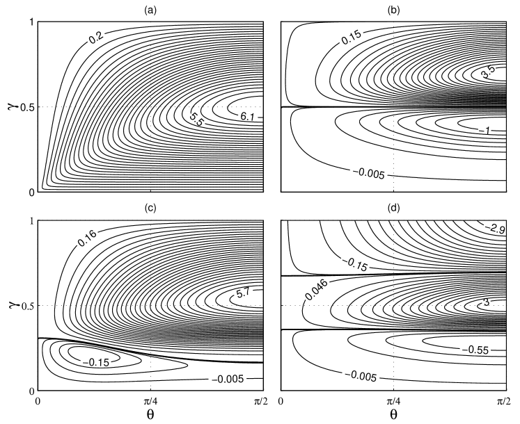
Figure 5: Contours of magnetic flux across a cap on the horizon (latitude angle $\theta$ is measured from the rotation axis) of a magnetized black hole: (a) $a=e=0$; (b) $a=1$, $e=0$; (c) $a=0.2$, $e=0$; (d) $a=-e=1/\sqrt{2}$ (electric charge and spin of the black hole). Here, $\gamma\equiv\left(1+\beta\right)^{-1}$, $\beta\equiv B_{0}M$. This figure from Karas & Budínová (2000) illustrates strong-gravity effects on magnetic fields that do not occur in weak-magnetic (test) field approximation, namely, the expulsion of the magnetic flux as a function of the intensity of the imposed magnetic field.

The electromagnetic field can be written in terms of orthonormal LNRF components,

$$H_{(r)}+{{\rm{i}}}E_{(r)} = A^{-1/2}\sin^{-1}\!\theta\,\Phi^{\prime}_{,\theta},$$

$$H_{(\theta)}+{{\rm{i}}}E_{(\theta)} = -\left(\Delta/A\right)^{1/2}\sin^{-1}\!\theta\,\Phi^{\prime}_{,r},$$

where $\Phi^{\prime}(r,\theta)=\Lambda^{-1}\left(\Phi-\frac{1}{2}\beta\mathcal{E}\right)$. The horizon is positioned at $r{\equiv}r_{+}=1+\sqrt{(}1-a^{2}-e^{2})$, independent of $\beta$. As in the non-magnetized case, the horizon exists only for $a^{2}+e^{2}\leq 1$.

There is an issue with this solution, namely, the range of angular coordinates versus the problem of conical singularity: $0\leq\theta\leq\pi$, $0\leq\phi<2\pi|\Lambda_{0}|^{2}$, where

$$|\Lambda_{0}|^{2}\equiv|\Lambda(\sin\theta=0)|^{2}=1+\textstyle{\frac{3}{2}}\beta^{2}e^{2}+2\beta^{3}ae+\beta^{4}\left(\textstyle{\frac{1}{16}}e^{4}+a^{2}\right).$$ (130)

The total electric charge $Q_{\rm{H}}$ and the magnetic flux $\Phi_{\rm{m}}(\theta)$ across a cap in axisymmetric position on the horizon (with the edge defined by $\theta={\rm{const}}$):

$$Q_{\rm{H}} = -|\Lambda_{0}|^{2}\,\Im{\rm{m}\,}\Phi^{\prime}\left(r_{+},0\right),$$

$$\Phi_{\rm{m}} = 2\pi|\Lambda_{0}|^{2}\,\Re{\rm{e}\,}\Phi^{\prime}\left(r_{+},\bar{\theta}\right)\Bigr{|}^{\theta}_{\bar{\theta}=0}.$$

The magnetic flux across the black hole hemisphere in the exact magnetized black hole solution is shown in fig. 5.

The author acknowledges continued support from the Czech Science Foundation grant No. 13-00070J.

References

- (1) Adámek K., Stuchlík Z. (2013), “Magnetized tori in the field of Kerr superspinars”, Class. Quantum Grav., 30 205007
- (2) Alekseev G. A., Garcia A. A. (1996), “Schwarzschild black hole immersed in a homogeneous electromagnetic field”, Phys. Rev. D 53, 1853
- (3) Bičák J., Dvořák L. (1980), “Stationary electromagnetic fields around black holes. III.”, Phys. Rev. D, 22, 2933
- (4) Bičák J., Karas V. (1989), “The influence of black holes on uniform magnetic fields”, in Proc. of the 5th Marcel Grossman Meeting on General Relativity, eds. D. G. Blair & M. J. Buckingham (Singapore: World Scientific), p. 1199
- (5) Bičák J., Ledvinka T. (2000), “Electromagnetic fields around black holes and Meissner effect”, Nuovo Cim., B115, 739
- (6) Bullard E. C. (1949), “Electromagnetic induction in a rotating sphere”, Proc. Roy. Soc. Lond., 199, 413
- (7) Chandrasekhar S. (1983), The Mathematical Theory of Black Holes (Oxford: Oxford University Press)
- (8) Christodoulou D., Ruffini R. (1973), “On the electrodynamics of collapsed objects”, in Black Holes, eds. C. DeWitt & B. S. DeWitt (New York: Gordon and Breach Science Publishers), p. R151
- (9) Dovčiak M., Karas V., Lanza A. (2000), “Magnetic fields around black holes”, European Journal of Physics, 21, 303
- (10) Elsasser W. M., “The Earth’s interior and geomagnetism”, Rev. Mod. Phys., 22, 1
- (11) Ernst F. J., and Wild W. J. (1976), “Kerr black holes in a magnetic universe”, J. Math. Phys., 12, 1845
- (12) Gal’tsov D. V. (1986), Particles and Fields around Black Holes (Moscow: Moscow University Press)
- (13) Hiscock W. A. (1981), “On black holes in magnetic universes”, J. Math. Phys., 22, 1828
- (14) Karas V. (1989), “Asymptotically uniform magnetic field near a Kerr black hole”, Phys. Rev. D, 40, 2121
- (15) Karas V. (2005), “An introduction to relativistic magnetohydrodynamics. I. The force-free approximation”, in Proceedings of RAGtime 6/7: Workshops on black holes and neutron stars, eds. S. Hledík and Z. Stuchlík (Opava: Silesian University), pp. 71–80; Paper I
- (16) Karas V., Budínová Z. (2000), “Magnetic fluxes across black holes in a strong magnetic field regime”, Physica Scripta, 61, 253
- (17) Karas V., Kopáček O. (2009), “Magnetic layers and neutral points near a rotating black hole”, Class. Quantum Grav., 26, 025004
- (18) Karas V., Kopáček O., Kunneriath D. (2012), “Influence of frame-dragging on magnetic null points near rotating black holes”, Class. Quantum Grav., 29, id. 035010
- (19) Karas V., Kopáček O., Kunneriath D. (2013), “Magnetic Neutral Points and Electric Lines of Force in Strong Gravity of a Rotating Black Hole”, International Journal of Astronomy and Astrophysics, 3, 18
- (20) Karas V., Kopáček O., Kunneriath D., Hamerský, J. (2014), “Oblique magnetic fields and the role of frame dragging near rotating black hole”, Acta Polytechnica, in press (arXiv:1408.2452)
- (21) Karas V., Vokrouhlický D. (1990), “On interpretation of the magnetized Kerr-Newman black hole”, J. Math. Phys., 32, 714
- (22) King A. R., Lasota J. P., Kundt W. (1975), “Black holes and magnetic fields”, Phys. Rev. D, 12, 3037
- (23) Kramer D., Stephani H., MacCallum M., and Herlt E. (1980), Exact Solutions of the Einstein’s Field Equations (Berlin: Deutscher Verlag der Wissenschaften)
- (24) Nathanail A. Contopoulos I. (2014), “Black hole magnetospheres”, ApJ, 788, id. 186
- (25) Newman E. T., Penrose R. (1962), “An approach to gravitational radiation by a method of spin coefficients”. Journal of Mathematical Physics, 3, 566
- (26) Ortaggio M. (2005), “Higher dimensional black holes in external magnetic fields”, Journal of High Energy Physics, Issue 05, id. 048
- (27) Penna, R. F. (2014), “Black hole Meissner effect and Blandford-Znajek jets”, Physical Review D, 89, id. 104057
- (28) Punsly B. (2008), Black Hole Gravito-hydromagnetics (Berlin: Springer-Verlag)
- (29) Teukolsky S. (1973), “Perturbations of a rotating black hole”, ApJ, 185, 635
- (30) Thorne K. S., Price R. H., and Macdonald, D. A. (1986), Black Holes: The Membrane Paradigm (New Haven: Yale University Press)
- (31) Wald R. M. (1974), “Black hole in a uniform magnetic field”, Phys. Rev. D, 10, 1680
- (32) Wald R. M. (1984), General Relativity (Chicago: University of Chicago Press)
- (33) Yazadjiev S. S. (2006), “Magnetized black holes and black rings in the higher dimensional dilaton gravity”, Physical Review D, 73, id. 064008