Causal horizons and some topics concerning structure formation

Abstract

This is a write-up of a talk given at the Opava RAGtime meeting in 2011, but it has been updated to include some subsequent related developments. The talk focused on discussion of some aspects of black hole and cosmological horizons under rather general circumstances, and on two different topics related to formation of cosmological structures at different epochs of the universe: virialization of cold dark matter during standard structure formation in the matter-dominated era, and primordial black hole formation during the radiative era.

1 Introduction

This presentation focuses firstly on two different types of causal horizon: those for black holes (where no causal signal can get out from inside), and that for the universe (where no causal signal can get in from outside). Also, we discuss some topics connected with formation of structure in the universe in the matter-dominated and radiative eras. We follow the convention of using units for which $c=G=1$ except in section 3.1, where the treatment is entirely Newtonian and it is convenient to retain $G$.

In all of these discussions, we will make the (major) simplification of considering just spherical symmetry but, apart from that, we will remain rather general. We start from the Friedman-Robertson-Walker metric for describing a homogeneous and isotropic background universe and we use the spatially-flat form of it, in line with current observations:

$$\mathrm{d}s^{2}=-\mathrm{d}t^{2}+S^{2}(t)\left[\mathrm{d}r^{2}+r^{2}\left(\mathrm{d}\theta^{2}+\sin^{2}\theta\mathrm{d}\varphi^{2}\right)\right]\,,$$ (1)

where $r$ is a co-moving radial coordinate and $S(t)$ is the scale factor. This can be written in the alternative form

$$\mathrm{d}s^{2}=-\mathrm{d}t^{2}+S^{2}(t)\mathrm{d}r^{2}+R^{2}\left(\mathrm{d}\theta^{2}+\sin^{2}\theta\mathrm{d}\varphi^{2}\right)\,,$$ (2)

where $R=S(t)r$ is a circumference coordinate (invariantly defined as being the proper circumference of a circle, centred on the origin, divided by $2\pi$). This is the same quantity as used for the radial coordinate in the standard form of the Schwarzschild metric.

The above description is for a uniform medium; when we have a (spherically symmetric) deviation away from this, the metric can then be written in the generalised form

$$\mathrm{d}s^{2}=-a^{2}\mathrm{d}t^{2}+b^{2}\mathrm{d}r^{2}+R^{2}\left(\mathrm{d}\theta^{2}+\sin^{2}\theta\mathrm{d}\varphi^{2}\right)\,,$$ (3)

with $a$, $b$ and $R$ all being functions of $r$ and $t$. Using a diagonal form of the metric like this (with no cross terms involving $\mathrm{d}r\,\mathrm{d}t$, etc.) implies a particular choice of time slicing, and the time coordinate here is often called “cosmic time”. The form of metric (3) can be used in principle for any spherically-symmetric space-time, although it is often more convenient in practice to use other kinds of slicing.

2 Causal horizons

In this section, we discuss how the concepts of black-hole and cosmological horizons emerge from a general treatment of outgoing and ingoing null rays. We continue to assume spherical symmetry and take the medium to be a perfect fluid, but our discussion is general in the sense that it is independent of the equation of state used for the matter and we make no assumptions of homogeneity (with reference to the cosmological case), or of stationarity, asymptotic flatness and the presence of vacuum exteriors (with reference to the black holes). It can be interesting to see how well-known results emerge in this approach.

First, we consider the general treatment of radial null rays, using the cosmic time form of the metric (3) introduced above. Along the path of any radial null ray, we have $\mathrm{d}s=\mathrm{d}\theta=\mathrm{d}\phi=0$ and so

$$\mathrm{d}r=\pm\,\frac{a}{b}\,\mathrm{d}t\,,$$ (4)

with the plus corresponding to an outgoing ray and the minus to an ingoing one. Note that here “outgoing” and “ingoing” are defined with respect to the comoving frame of local matter. This convention is used throughout the present section.

The general expression for changes in $R$ along a radial worldline is

$$\mathrm{d}R=\frac{\partial R}{\partial t}\,\mathrm{d}t+\frac{\partial R}{\partial r}\,\mathrm{d}r\,,$$ (5)

and so along a radial null ray

$$\mathrm{d}R=\left(\frac{\partial R}{\partial t}\pm\frac{a}{b}\frac{\partial R}{\partial r}\right)\mathrm{d}t\,.$$ (6)

Following the classic paper of Misner (1969), we now introduce the operators

$$D_{t}\equiv\frac{1}{a}\,\frac{\partial}{\partial t}\qquad{\rm and}\qquad D_{r}\equiv\frac{1}{b}\,\frac{\partial}{\partial r}\,.$$ (7)

Applying these to the circumference coordinate $R$, one then defines the quantities

$$U\equiv D_{t}R\qquad{\rm and}\qquad\Gamma\equiv D_{r}R\,,$$ (8)

where $U$ is the radial component of four-velocity in the “Eulerian” frame, with respect to which the fluid is moving, and $\Gamma$ is a generalized Lorentz factor (which reduces to the standard one in the special relativistic limit). In terms of these,

$$\frac{\partial R}{\partial t}=aU\qquad{\rm and}\qquad\frac{\partial R}{\partial r}=b\Gamma\,.$$ (9)

Inserting these into equation (6) gives the expression for how $R$ changes with time along a radial null ray:

$$\frac{\mathrm{d}R}{\mathrm{d}t}=a\left(U\pm\Gamma\right)\,,$$ (10)

where the plus is again for a ray which is outgoing (with respect to the matter) while the minus is for an ingoing one.

To find an expression for $\Gamma$, we need to use the Einstein field equation. As usual, we approximate the matter to behave as a perfect fluid with the stress-energy tensor

$$T^{\mu\nu}=(e+p)u^{\mu}u^{\nu}+pg^{\mu\nu}\,,$$ (11)

where $e$ is the energy density, $p$ is the pressure and $u^{\mu}$ is the four-velocity. The $G^{0}_{0}$ and $G^{1}_{1}$ components of the Einstein equation then give

$$4\pi R^{2}eR_{,r}=\textstyle{\frac{1}{2}}\left(R+RU^{2}-R\Gamma^{2}\right)_{,r}\,,$$ (12)

and

$$4\pi R^{2}apU=-\textstyle{\frac{1}{2}}\left(R+RU^{2}-R\Gamma^{2}\right)_{,t}\,,$$ (13)

with the commas representing partial derivatives. It is convenient to make the definition

$$m\equiv\textstyle{\frac{1}{2}}\left(R+RU^{2}-R\Gamma^{2}\right)\,.$$ (14)

Integrating equation (12) then gives

$$m=\int 4\pi R^{2}e\,\mathrm{d}R\,,$$ (15)

(corresponding to the interpretation of $m$ as the mass contained within radius $R$), while equation (13) gives

$$D_{t}m=-4\pi R^{2}pU\,,$$ (16)

(representing the change of energy resulting from work done against pressure during expansion or contraction). Rearranging the terms in (14) then gives

$$\Gamma^{2}=1+U^{2}-\frac{2m}{R}\,.$$ (17)

Returning now to equation (10), the limiting surface at which an outgoing radial light ray cannot move to larger $R$, is given by

$$\left(\frac{\mathrm{d}R}{\mathrm{d}t}\right)_{\rm\!out}=a(U+\Gamma)=0\,,$$ (18)

implying

$$\Gamma=-U\,.$$ (19)

This corresponds to the so-called “apparent horizon” of a black hole. Similarly, the limiting surface at which an ingoing radial light ray cannot move to smaller $R$ is given by

$$\left(\frac{\mathrm{d}R}{\mathrm{d}t}\right)_{\rm\!in}=a(U-\Gamma)=0\,,$$ (20)

implying

$$\Gamma=U\,.$$ (21)

This corresponds to the cosmological (Hubble) horizon. Note that the surfaces for which (19) and (21) hold are marginally trapped surfaces and so are representations of a concept (Penrose, 1965) which plays a fundamental role in general relativity.

Conditions (19) and (21) are different, of course, but for both of them

$$\Gamma^{2}=U^{2}\,,$$ (22)

and so, using (17), they both correspond to the condition

$$R=2m\,,$$ (23)

which is a familiar result! Although we have used cosmic-time slicing in this derivation, the final result is actually independent of the slicing used. We stress again that our derivation here does not depend on any assumptions of homogeneity (with reference to the cosmological case), or of stationarity, asymptotic flatness and the presence of vacuum exteriors (with reference to black holes).

3 Cosmological structure formation

In this section, we discuss some topics concerning cosmological structure formation at two different stages in the history of the universe: in the matter-dominated and radiative eras. The main interest is in the consequences of perturbations which started as small quantum fluctuations in the very early universe and were then inflated onto supra-horizon scales, eventually re-entering the horizon as the universe continued to expand, and becoming causally connected again. (“Horizon” here refers to the cosmological horizon.) We focus on the case of an over-density surrounded by a compensating under-density. Once the over-density has re-entered the horizon, there is a possibility that it could then evolve into a persisting condensed structure. A perturbation originating at a very early time, such as those mentioned above, may have begun with a mixture of growing and decaying components, but any decaying part would soon have faded away so that by the time of horizon re-entry, only the growing part would remain. Growing-modes are special; they have a particular combination of density and velocity perturbation which makes them “hold together” as they evolve.

We discuss below the re-entry of perturbations during the matter-dominated era, when the matter is commonly described as pressureless, with $p=0$ (although we will have more to say about that), and during those parts of the radiative era (defined as being when only relativistic zero-rest-mass particles are important) in which $p=\frac{1}{3}e$ is a good approximation. The first case can lead to formation of galactic or pre-galactic equilibrium structures, whereas in the second case primordial black holes (on a much smaller scale) are the only condensed structures that can be formed.

3.1 Virialization in the matter-dominated era

Cosmologists like to use equations of state of the form $p=we$, where $w$ is a constant. The cases $p=\frac{1}{3}e$ and $p=0$ do fit with this, of course, but it is questionable whether taking $p=0$ actually makes sense in general for the matter-dominated era. For calculating the evolution of a uniform background universe, it is indeed satisfactory, but it becomes problematic when dealing with structure formation beyond the regime of linear perturbations. For cold dark matter (CDM) particles, it is frequently said that they must be pressureless because of being effectively collisionless, but this misses the point that pressure comes from the random motion of particles and is only indirectly influenced by collisions between them. If CDM particles have a non-zero velocity dispersion, then they automatically have a non-zero pressure and this is generally not irrelevant even if it may be small. The role of collisions is in assisting the particle distribution function to relax towards an isotropic Maxwellian, not directly in producing the pressure. A completely collisionless medium can certainly have a finite pressure (although that will generally not be isotropic).

In this subsection, we investigate the phenomenology of the “turn-round radius” and the “virialization radius” for perturbations when they re-enter the cosmological horizon and begin to feel their self-gravity. Initially, the over-density is continuing to expand along with the rest of the universe (although slightly more slowly because of the velocity perturbation in a growing mode) but, as it progressively begins to feel its self-gravity more, it slows down further and eventually reverses its expansion into a contraction. Its radius when that happens is called the turn-round radius. We will follow here just the subsequent behaviour of the dark matter component, which is more or less collisionless. As the contraction proceeds, the random velocities of the constituent particles progressively increase until eventually the effect of their random motions is sufficient to balance gravity (possibly aided by rotation) and the configuration settles into an equilibrium state. Its radius then is called the virialization radius (we explain this more below). In numerical simulations, it is often found that this virialization radius is roughly half of the turn-round radius.

Clearly, structure formation is in general a three-dimensional problem, but could one get a reasonable approximate picture for the above process by using a simple spherically-symmetric toy model? If so, that could be useful for trial inclusion of further effects (dynamical scalar fields, etc.). Our idea is to include the random motions of the CDM particles in terms of an effective temperature $T$ and insert that into a model equation of state, giving a pressure $p$. We proceed as follows. CDM particles are non-relativistic and so the thermal energy per particle is given by

$$u=\textstyle{\frac{3}{2}}\,k_{B}T\,,$$ (24)

(assuming local isotropy; $k_{B}$ is Boltzmann’s constant). The thermal energy density is then

$$\rho\varepsilon=\textstyle{\frac{3}{2}}\,nk_{B}T\,,$$ (25)

(where $\rho$ is the rest-mass density, $\varepsilon$ is the specific internal energy, and $n$ is the particle number density). The ideal gas law $p=nk_{B}T$ then gives

$$p=\textstyle{\frac{2}{3}}\,\rho\varepsilon\,,$$ (26)

which leads to

$$p=K(s)\rho^{5/3}\,,$$ (27)

using the first law of thermodynamics. This is the well-known polytropic relation for a monatomic non-relativistic gas (here $K(s)$ is a function of the specific entropy $s$ and goes to a constant for adiabatic processes).

Next, we recall the considerations leading to a simple form of the virial theorem, following Tayler (1970). (Note that the treatment in this subsection is entirely Newtonian and it is convenient to retain the $G$ in the equations for this part; also $r$ is here the standard classical radial coordinate.) The equation of hydrostatic equilibrium

$$\frac{\mathrm{d}p}{\mathrm{d}r}=-\frac{Gm\rho}{r^{2}}\,,$$ (28)

where $m$ is the mass contained within radius $r$, can be rearranged to give

$$4\pi r^{3}\mathrm{d}p=-\left(\frac{Gm}{r}\right)4\pi r^{2}\rho\,\mathrm{d}r\,.$$ (29)

We now integrate equation (29) over the volume of the spherical object:

$$\int{3V\,\mathrm{d}p}=\int{\Phi\,\mathrm{d}m}\,,$$ (30)

where $V$ is the volume contained within radius $r$ and $\Phi=-(Gm/r)$ is the gravitational potential at radius $r$. Integrating the left-hand side by parts then gives

$$3\Big{[}pV\Big{]}-3\int{p\,\mathrm{d}V}=\Omega\,,$$ (31)

where $\Omega$ is the gravitational potential energy of the object. Taking the pressure at the surface to be zero and inserting the equation of state expression (26) for $p$, one obtains

$$-3\int{\textstyle{\frac{2}{3}}\,\rho\varepsilon\,\mathrm{d}V}=-2U=\Omega\,,$$ (32)

where $U$ is the total internal energy of the object. The overall total energy is then

$$E=U+\Omega=\textstyle{\frac{1}{2}}\,\Omega\,,$$ (33)

which is negative, as it must be for a gravitationally-bound object. When equation (33) is satisfied, the configuration is said to be virialized.

We will now use these ideas for studying the issue of the turn-round radius and virialization radius within our simple toy model. We will use the subscripts ${tr}$ and $v$ to denote “turn-round” and “virial” respectively. The configuration starts off (at the turn-round radius $R_{tr}$) out of hydrostatic equilibrium and not satisfying equation (33). As the contraction proceeds, the pressure plays an increasing role in counteracting gravity until eventually equilibrium is reached and the virial condition (33) is satisfied. The radius at which this happens is the virialization radius ($R_{v}$) mentioned earlier.

Assuming conservation of the total energy during the contraction,

$$E=U_{v}+\Omega_{v}=U_{tr}+\Omega_{tr}\,.$$ (34)

At the turn-round radius, the energy in the random motions of the CDM particles is still going to be small (it grows later as the contraction proceeds) and so it seems safe to assume that the initial total internal energy term $U_{tr}$ can be neglected. Doing this, and using expression (33) at the virial radius, we have

$$E=\textstyle{\frac{1}{2}}\,\Omega_{v}=\Omega_{tr}\,.$$ (35)

If we now make the (rough) assumptions that the total mass $M$ does not change during the contraction and that, throughout, we can write

$$\Omega=-\frac{GM^{2}}{R}\times{\rm constant}\,,$$ (36)

then $\frac{1}{2}\Omega_{v}=\Omega_{tr}$ gives

$$\frac{GM^{2}}{2R_{v}}=\frac{GM^{2}}{R_{tr}}\,,$$ (37)

and so

$$R_{v}=\textstyle{\frac{1}{2}}R_{tr}\,,$$ (38)

in agreement with the numerical results.

Our purpose here has been to suggest that this type of “fluid” treatment of cold dark matter might be a useful approach in some circumstances. Clearly, implementations could be made much more detailed than the one which we have sketched above.

3.2 The radiative era and primordial black holes

Objects composed of matter for which $p=\frac{1}{3}e$ have an adiabatic index of $4/3$ and are fundamentally unstable. Because of this, collapsing perturbations in the radiative era do not produce equilibrium condensed structures, but either form black holes (if the perturbation amplitude $\delta$ is greater than a certain critical threshold value $\delta_{c}$) or bounce and return back into the roughly uniform medium from which they came. Black holes formed then could have lower masses than ones formed today by the collapse of stars. Since this type of matter has no intrinsic scale, the question arises of whether the phenomenon known as “critical collapse” (Choptuik, 1993) might occur under these circumstances despite the background being that of the expanding universe. The standard form of critical collapse is characterised by the property that, for values of $(\delta-\delta_{c})$ which are positive but sufficiently small, the mass of the black hole formed, $M_{BH}$, is related to $(\delta-\delta_{c})$ by a scaling law, i.e.

$$M_{BH}\propto\left(\delta-\delta_{c}\right)^{\gamma}\,,$$ (39)

(with $\gamma$ being a constant) when the nature of the unperturbed background is kept fixed and the perturbations introduced differ in amplitude but not in shape. This sort of behaviour has been seen in quite a wide range of numerical simulations treating idealised circumstances (see the review by Gundlach and Martín-García, 2007) but its occurrence under “real-world” circumstances is less clear. It seemed possible that the radiative era of the early universe might provide an arena for this, although a potential problem comes from the fact that the universe itself has an intrinsic scale (the cosmological horizon scale) which might or might not interfere with the scaling behaviour. Niemeyer and Jedamzik (1999) made calculations which demonstrated the presence of a scaling law under these circumstances over a restricted range of $(\delta-\delta_{c})$ but when more extensive calculations were made, going closer to the critical limit (Hawke and Stewart, 2002), it was found that the scaling law eventually broke as the behaviour became more extreme near to the critical limit. We then reinvestigated this ourselves (Musco et al., 2009), focusing particularly on the use of perturbations containing only a growing-mode component (following on from the discussion at the beginning of Section 3). For our calculations, we used a purpose-built numerical GR hydro code implementing an AMR technique within a null-slicing approach, and able to go down to extremely small values of $(\delta-\delta_{c})$. Using growing-mode initial data, without any decaying component (following the methodology of Polnarev and Musco, 2007), we found that the scaling behaviour did go all the way down to the smallest values of $(\delta-\delta_{c})$ that we were able to treat, well beyond the breaking point found previously. Results are shown in Figure 1. In our work, we define $\delta$ as being the relative mass excess inside the over-dense region at the time when it re-enters the cosmological horizon, and measure $M_{BH}$ in units of $M_{H}$, the cosmological horizon mass at that time, so that the results are independent of epoch within the radiative era. Note that black holes produced like this would have typically lower masses when formed earlier rather than later (related with the value of $M_{H}$ at the time).

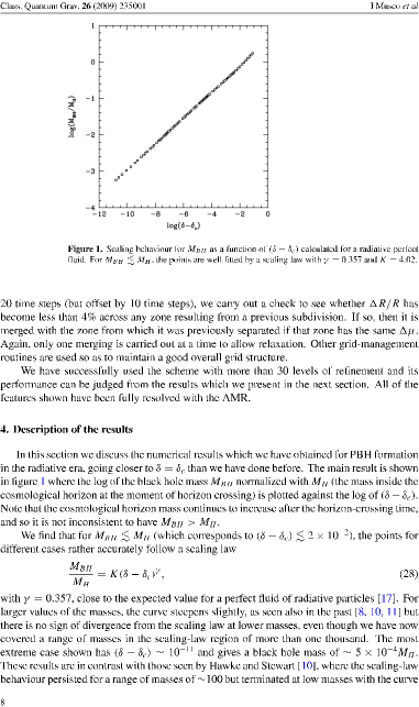
Figure 1: Scaling behaviour for $M_{BH}$ as a function of $(\delta-\delta_{c})$. $M_{BH}$ is measured in units of $M_{H}$, the mass within the cosmological horizon when the perturbation re-enters it. For $M_{BH}\lesssim M_{H}$, the points are well fitted by a scaling law with $\gamma=0.357$, which matches well with the corresponding result obtained semi-analytically by Maison (1996) for standard critical collapse with this type of matter.

Figure 2: Simulation results for the velocity $U$ (from a run with $\delta-\delta_{c}\sim 10^{-9}$) plotted against the similarity coordinate $\xi=R/(t_{c}-t)$. The plot shows curves for a succession of times during the close approach to the similarity solution, with the higher peaks corresponding to the later times. The precise similarity solution for the collapsing matter is marked with the dashed curve, which is partly covered by the solid curves.

In the literature on critical collapse, a key feature is the occurrence of similarity solutions accompanying the scaling laws (Evans and Coleman, 1994). As $(\delta-\delta_{c})\to 0$, a critical solution is approached where all of the matter in the original contracting region is progressively shed during the contraction which ends, with zero matter, at a time referred to as the critical time $t_{c}$. The later stages of this follow a similarity solution. For small positive values of $(\delta-\delta_{c})$, the similarity solution is closely approached but eventually there is a divergence away from it, with the remaining material then collapsing to form a black hole. It is interesting to see how this plays out in our case, where the collapse occurs within the background of an expanding universe. We have investigated this in some detail (Musco and Miller, 2013). Figure 2 shows our results from a run with $\delta-\delta_{c}\sim 10^{-9}$, which is rather close to the critical limit; the four-velocity $U$ is plotted as a function of the similarity coordinate $\xi=R/(t_{c}-t)$ at a succession of times (solid curves), with the higher peaks corresponding to the later times. Note the shedding of material occurring via a relativistic wind. One can see the progressive approach of the simulation results towards the similarity solution (dashed curve), with the range of the zone of agreement increasing with time. At the last time shown, the similarity solution is being closely approximated over all of the contracting region, where $U$ is negative (although it is quite hard to see this as being negative in the figure because of the scale), and also over the part of the surrounding region out to the maximum of $U$; beyond this, the simulation results diverge completely away from the similarity solution and eventually merge into the surrounding Friedmann-Robertson-Walker universe. The similarity behaviour breaks soon after the last time shown here, with the start of the final collapse leading to black hole formation. We should stress that the use of a logarithmic coordinate in Figure 2 has the effect of making features appear much more abrupt than they would do with a standard linear coordinate. The almost vertical parts of the curves are nowhere near to being shocks and correspond to smoothly varying features when viewed on a linear scale.

4 Conclusions

We have touched here on a number of topics. Firstly, a unified treatment has been given of black-hole and cosmological horizons in terms of co-moving trapped surfaces. This does not depend on any assumptions of homogeneity (in the cosmological case), or of stationarity, asymptotic flatness and the presence of vacuum exteriors (for the black holes). We then went on to discuss two topics concerned with cosmological structure formation: virialization of cold dark matter during standard structure formation in the matter-dominated era, and primordial black hole formation during the radiative era. In the first case, we presented a simple toy model which serves as an analytic demonstration of phenomena observed in numerical simulations; in the second case, we presented results showing that black-hole formation by collapse of cosmological perturbations in the radiative era completely follows the well-known phenomenology of critical collapse, as long as the perturbations are of the growing-mode type when they re-enter the cosmological horizon.

The research of Ilia Musco is currently being supported by postdoctoral funding from ERC-StG EDECS contract no. 279954.

References

- Choptuik (1993) Choptuik, M.W. (1993), Phys. Rev. Lett., 70, 9.
- Evans and Coleman (1994) Evans, C.R. and Coleman, J.S. (1994), Phys. Rev. Lett., 72, 1782.
- Gundlach and Martín-García (2007) Gundlach, C. and Martín-García, J.M. (2007), Living Rev. Relativity, 10, 5, URL http://www.livingreviews.org/lrr-2007-5.
- Hawke and Stewart (2002) Hawke, I. and Stewart, J.M. (2002), Class. Quantum Grav., 19, 3687.
- Maison (1996) Maison, D. (1996), Phys. Lett. B, 366, 82.
- Misner (1969) Misner, C.W. (1969), in M. Chrétien, S. Deser and J. Goldstein, editors, Astrophysics and General Relativity, Volume 1, 1968 Brandeis University Summer Institute in Theoretical Physics, p. 113, Gordon and Breach, New York.
- Musco and Miller (2013) Musco, I. and Miller, J.C. (2013), Class. Quantum Grav., 30, 145009.
- Musco et al. (2009) Musco, I., Miller, J.C. and Polnarev, A.G. (2009), Class. Quantum Grav., 26, 235001.
- Niemeyer and Jedamzik (1999) Niemeyer, J.C. and Jedamzik, K. (1999), Phys. Rev. D, 59, 124013.
- Penrose (1965) Penrose, R. (1965), Phys. Rev. Lett., 14, 57.
- Polnarev and Musco (2007) Polnarev, A.G. and Musco, I. (2007), Class. Quantum Grav., 24, 1405.
- Tayler (1970) Tayler, R.J. (1970), The stars: their structure and evolution, p. 55, Wykeham, London.