Revisiting correlations between broad-line and jet emission variations for AGNs: 3C 120 and 3C 273

Abstract

We restudy the issue of cross-correlations between broad-line and jet emission variations, and aim to locate the position of radio (and gamma-ray) emitting region in jet of active galactic nuclei (AGNs). Considering the radial profiles of the radius and number density of clouds in a spherical broad-line region (BLR), we derive new formulae connecting jet emitting position $R_{\rm{jet}}$ to time lag $\tau_{\rm{ob}}$ between broad-line and jet emission variations, and BLR radius. Also, formulae are derived for a disk-like BLR and a spherical shell BLR. The model-independent FR/RSS method is used to estimate $\tau_{\rm{ob}}$. For 3C 120, positive lags of about 0.3 yr are found between the 15 GHz emission and the H$\beta$, H$\gamma$ and He II $\lambda 4686$ lines, including broad-line data in a newly published paper, indicating the line variations lead the 15 GHz ones. Each of the broad-line light curves corresponds to a radio outburst. $R_{\rm{jet}}=$1.1–1.5 parsec (pc) are obtained for 3C 120. For 3C 273, a common feature of negative time lags is found in the cross-correlation functions between light curves of radio emission and the Balmer lines, and as well Ly$\alpha\/\ \lambda 1216$ and C iv $\lambda 1549$ lines. $R_{\rm{jet}}=$ 1.0–2.6 pc are obtained for 3C 273. The estimated $R_{\rm{jet}}$ are comparable for 3C 120 and 3C 273, and the gamma-ray emitting positions will be within $\sim$ 1–3 pc from the central engines. Comparisons show that the cloud number density and radius radial distributions and the BLR structures only have negligible effects on $R_{\rm{jet}}$.

1 INTRODUCTION

According to the reverberation mapping model (e.g. Blandford & McKee, 1982), the broad emission line variations follow the ionizing continuum variations through the photoionization process. The variability correlations between the continuum and broad emission lines of active galactic nuclei (AGNs) have been studied over the last decades (e.g. Kaspi & Netzer, 1999; Kaspi et al., 2000; Peterson et al., 2005). A review about the reverberation mapping researches is given in Gaskell (2009, and references therein). The jets can be ejected from inner accretion disk in the vicinity of black hole (e.g. Penrose, 1969; Blandford & Znajek, 1977; Blandford & Payne, 1982; Meier et al., 2001). The disturbances in the central engine are likely propagated outwards along the jets. Observations show that dips in the X-ray emission, generated in the central engine, are followed by ejections of bright superluminal radio knots in the jets of AGNs and microquasars (e.g. Marscher et al., 2002; Arshakian et al., 2010). The dips in the X-ray emission are well correlated with the ejections of bright superluminal knots in the radio jets of 3C 120 (Chatterjee et al., 2009) and 3C 111 (Chatterjee et al., 2011). The outbursts are physically linked to the ejections of superluminal knots (e.g. Türler et al., 2000). These outbursts of broad-line and jet emission should respond to the stronger disturbances in the central engine. Cross-correlations between broad-line and jet emission variations are expected, and a new method was proposed to explain these correlations and constrain the positions of radio and gamma-ray emitting regions (Liu et al., 2011a, hereafter Paper I).

A ring broad-line region (BLR) is assumed to be perpendicular to the jet axis (Paper I). This ring configuration of BLR is a toy model relative to a disk-like BLR. Several groups find evidence for disk-like BLRs (e.g. Kollatschny et al., 2003; Pozo Nuñez et al., 2013, and references therein). A necessary requirement of this disk-like BLR is to have good variation features in the light curves. This is especially the case for 3C120, as reported in Pozo Nuñez et al. (2014). The sharp variation features are present in both the AGN continuum and the BLR echo, and evidence for a nearly face-on disk-like BLR geometry with an inclination of 10 degrees has been found for 3C120. The disk-like BLR is also used to explain the double-peaked broad-lines in some AGNs, e.g. 3C 390.3 (Zhang, 2013). A spherical BLR with some thickness is a widely used configuration for the researches of the broad-line variability in AGNs (e.g. Kaspi & Netzer, 1999). The spherical BLR is also used to study gamma-ray emission of AGNs (e.g. Bai et al., 2009; Liu & Bai, 2006; Liu et al., 2008; Tavecchio & Mazin, 2009). A spherical shell with a zero-thickness is used to study the origin of gamma-ray emission of blazars (Ghisellini & Madau, 1996). The spherical BLR consists of clouds with radial number density and radius pow-law profiles of $n_{\rm{c}}(r)\propto r^{-p}$ and $r_{\rm{c}}(r)\propto r^{q}$, respectively, where $r$ is the distance from the central engine to a cloud, and the pow-law indexes $p$ and $q$ are positive (e.g. Kaspi & Netzer, 1999). This spherical BLR cloud model can fit variable broad emission lines in AGNs. The BLR clouds may be bloated stars with extended envelopes, and the emission-line intensities, profiles, and variability can be fitted to the mean observed AGN spectrum under this model (Alexander & Netzer, 1994, 1997). These two BLR models have a good agreement in the trends of number density and density radial profiles of clouds (see Kaspi & Netzer, 1999).

3C 120 and 3C 111 are classified into the misaligned AGNs in the third catalog of AGNs detected by Fermi-LAT (Ackermann et al., 2015). The initial detection of 3C 120 with Fermi-LAT was reported by Abdo et al. (2010c). Over the past 2 yr, Fermi-LAT sporadically detected 3C 120 with high significance in the MeV/GeV band (Tanaka et al., 2015). Kataoka et al. (2011) argued that the gamma-ray emission of broad-line radio galaxies detected by Fermi-LAT are most likely produced in the inner nucleus jets rather than large scale jet structures. Broad-line blazar 3C 273 is brighter one of Fermi-LAT monitored sources, and is included in the first catalog of AGNs detected by Fermi-LAT (Abdo et al., 2010b). The gamma-ray flares detected with Fermi-LAT for 3C 273 give a limit of gamma-ray emitting position smaller than 1.6 parsec (pc) from the central engine (Rani et al., 2013). For 3C 120, it was concluded that the gamma rays in the MeV/GeV band are more favorably produced via the synchrotron self-Compton process, rather than inverse Compton scattering of external photons coming from BLR or dusty torus (Tanaka et al., 2015). The conclusion is based on their constraints on the relative positions of the gamma-ray and radio emission regions. Therefore, the gamma-ray production position is the key issue of how the gamma rays are produced.

The spherical BLR and the disk-like BLR are usually used to produce the soft seed photons in the external Compton (EC) model of gamma rays. The BLRs are important to gamma rays from blazars. This importance arises from two factors. One is that the seed photons from the BLR have significant influences on the EC spectrum (e.g. Tavecchio & Ghisellini, 2008; Lei & Wang, 2014b). The other is photon-photon absorption between the seed photons and the gamma-ray photons (see Sikora et al., 1994; Wang, 2000; Liu & Bai, 2006; Liu et al., 2008; Sitarek & Bednarek, 2008; Tavecchio & Ghisellini, 2008; Bai et al., 2009; Tavecchio & Mazin, 2009; Lei & Wang, 2014a). The location of gamma-ray emitting region relative to the BLR is the underlying factor that controls how and how much the two factors influence the gamma rays (Liu et al., 2014). For the disk-like BLR and the spherical (shell) BLR with the same size, the relative positions are different for the same gamma-ray emitting region in the jet. In this paper, the spherical BLRs with different cloud distributions will be focused on deriving new formulae to estimate the radio emitting positions $R_{\rm{jet}}$ from the time lags between variations of broad-lines and radio emission. As comparison, we will estimate $R_{\rm{jet}}$ for the case of the disk-like BLR, the spherical shell BLR and the ring BLR with a zero-thickness. Once $R_{\rm{jet}}$ is known, the gamma-ray emitting position $R_{\rm{\gamma}}$ could be constrained by $R_{\rm{jet}}$ for AGNs.

The structure of this paper is as follows. Section 2 presents method. Section 3 is for applications and contains three subsections: subsection 3.1 presents analysis of time lag, subsection 3.2 application to 3C 120, and subsection 3.3 application to 3C 273. section 4 is for variability amplitude. Section 5 is for discussion and conclusions.

2 METHOD

In Paper I, the BLR is assumed to be a ring, and the plane of BLR is assumed to be perpendicular to the jet axis. In this paper, we assumed a spherical BLR, a BLR structure usually used. First, a very thin spherical shell BLR is considered to get new equations. Second, a spherical BLR is taken into account to get new formulae. The geometrical structure is presented in Fig. 1 for the shell BLR. First, the viewing angle to the jet axis is assumed to be $\alpha=0$. As the disturbances from the central engine reach point E (see Fig. 1a), where the jet emission are produced, i.e. $R_{\rm{jet}}$=AE, the ionizing continuum photons travel from A to C, and the line photons travel from C to D in time interval $R_{\rm{jet}}/v_{\rm{d}}$. In the case, there is a zero-lag, and we have $(R_{\rm{BLR}}+R_{\rm{jet}}-R_{\rm{BLR}}\cos\theta)/c=R_{\rm{jet}}/v_{\rm{d}}$. Then we have for point C

$$R_{\rm{jet}}=\frac{R_{\rm{BLR}}(1-\cos\theta)}{\frac{c}{v_{\rm{d}}}-1},$$ (1)

where $\theta$ is the polar angle in spherical coordinates $(r,\theta,\varphi)$, $R_{\rm{BLR}}$ is the BLR size, $v_{\rm{d}}$ is the travelling speed of disturbances down the jet and $c$ is the speed of light.

If the disturbances reach point E and the line photons reach F, the lines will lag the jet emission (see Fig. 1a). We have $R_{\rm{BLR}}+R_{\rm{jet}}-R_{\rm{BLR}}\cos\theta-\tau c=R_{\rm{jet}}/v_{\rm{d}}c$, and then

$$R_{\rm{jet}}=\frac{R_{\rm{BLR}}(1-\cos\theta)-\tau c}{\frac{c}{v_{\rm{d}}}-1},$$ (2)

where $\tau$ is the time lag of lines relative to the jet emission. If the disturbances reach point E and the line photons reach G, the lines will lead the jet emission (see Fig. 1a). We have $R_{\rm{BLR}}+R_{\rm{jet}}-R_{\rm{BLR}}\cos\theta+\tau c=R_{\rm{jet}}/v_{\rm{d}}c$, and then

$$R_{\rm{jet}}=\frac{R_{\rm{BLR}}(1-\cos\theta)+\tau c}{\frac{c}{v_{\rm{d}}}-1},$$ (3)

where $\tau$ is the time lag of the jet emission relative to the lines.

Equations (1), (2), and (3) can be unified into

$$R_{\rm{jet}}=\frac{R_{\rm{BLR}}(1-\cos\theta)+\tau c}{\frac{c}{v_{\rm{d}}}-1},$$ (4)

where $\tau$ is zero, negative, and positive. As $\tau=0$, equation (4) becomes equation (1). As $\tau<0$, equation (4) becomes equation (2). As $\tau>0$, equation (4) becomes equation (3). Equations (1)–(4) are obtained only for point C on spherical shell of BLR (Fig. 1a). The observed line photons are from the shell of BLR, and then the observed lag is an ensemble average over all points of the shell. The surface element spanning from $\theta$ to $\theta+d\theta$ and $\varphi$ to $\varphi+d\varphi$ on a spherical surface at constant radius r is $dS_{\rm{r}}=r^{2}\sin\theta d\theta d\varphi$. Thus the differential solid angle is $d\Omega=dS_{\rm{r}}/r^{2}=\sin\theta d\theta d\varphi$. Equation (4) can be integrated over every point in the spherical surface of BLR, and then be averaged over $4\pi$. Finally, we have

$$R_{\rm{jet}}=\frac{R_{\rm{BLR}}+\frac{\langle\tau_{\rm{ob}}\rangle}{1+z}c}{\frac{c}{v_{\rm{d}}}-1},$$ (5)

where $\langle\tau_{\rm{ob}}\rangle$ is the ensemble average of $\tau_{\rm{ob}}$ over the spherical surface of BLR [and $\langle 1-\cos\theta\rangle_{\rm{d\Omega}}=\int_{0}^{2\pi}\int_{0}^{\pi}(1-\cos\theta)\sin\theta d\theta d\varphi/4\pi=1$], and $z$ is the redshift of source. Equation (5) is same as equation (4) in Paper I.

Equations(5) is obtained for the viewing angle $\alpha=0$, which is a special case. In general, $\alpha\neq 0$ (see Fig. 1b). As the disturbances reach point B, where the jet emission are generated, the ionizing continuum photons travel from point A to E and the line photons travel from point E to G (assuming point D is zero-lag point). Thus, we have $R_{\rm{jet}}c/v_{\rm{d}}=\rm{AE+ED+DG}$, where $\rm{AE}=R_{\rm{BLR}}$, $\rm{DG}=\tau c$, and $\rm{ED}=\rm{FC}=\rm{AC-AF}=R_{\rm{jet}}\cos\alpha-R_{\rm{BLR}}\cos\theta$ (see Fig. 1b). For point E in the spherical surface of BLR, we have $R_{\rm{jet}}c/v_{\rm{d}}=R_{\rm{jet}}\cos\alpha-R_{\rm{BLR}}\cos\theta+R_{\rm{BLR}}+\tau c$, and then

$$R_{\rm{jet}}=\frac{R_{\rm{BLR}}(1-\cos\theta)+\tau c}{\frac{c}{v_{\rm{d}}}-\cos\alpha},$$ (6)

which becomes equation (4) as $\alpha=0$. Calculating the ensemble average over $\theta$ and $\varphi$ in equation (6), we have

$$R_{\rm{jet}}=\frac{R_{\rm{BLR}}+\frac{\langle\tau_{\rm{ob}}\rangle}{1+z}c}{\frac{c}{v_{\rm{d}}}-\cos\alpha},$$ (7)

which becomes equation (5) as $\alpha=0$, and is same as equation (7) in Paper I. Here, $v_{\rm{d}}$ is equivalent to the bulk velocity of jet $v_{\rm{j}}$, and $\langle\tau_{\rm{ob}}\rangle\equiv\tau_{\rm{ob}}$ is the measured time lag of the jet emission relative to the broad lines. From the velocity $\beta=v_{\rm{j}}/c$ and the viewing angle $\alpha$, we have the apparent speed $\beta_{\rm{a}}=\beta\rm{sin\alpha}/(1-\beta\rm{cos\alpha})$, which gives $\beta=\beta_{\rm{a}}/(\beta_{\rm{a}}\rm{cos\alpha}+\rm{sin\alpha})$. Substituting the expression of $\beta$ for the velocity term in equation (7), we have

$$R_{\rm{jet}}=\frac{\beta_{\rm{a}}}{\sin\alpha}(R_{\rm{BLR}}+\frac{\langle\tau_{\rm{ob}}\rangle}{1+z}c),$$ (8)

where $\beta_{\rm{a}}$, $\alpha$, and $R_{\rm{BLR}}$ are measured from observations, and $\tau_{\rm{ob}}$ can be derived from the cross-correlations between the broad-line and jet emission light curves. On the other hand, if we have $R_{\rm{jet}}$, we can get $R_{\rm{BLR}}$ from

$$R_{\rm{BLR}}=R_{\rm{jet}}\frac{\sin\alpha}{\beta_{\rm{a}}}-\frac{\langle\tau_{\rm{ob}}\rangle}{1+z}c.$$ (9)

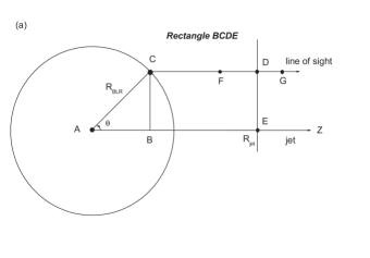
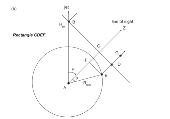
Figure 1: Sketch of axial cross section of the spherical geometry assumed, and it is similar to that used in the reverberation mapping method of broad emission lines. $R_{\rm{BLR}}$ is the size of BLR. ($a$) the angle between the line of sight and the jet axis $\alpha=0$. ($b$) $\alpha\neq 0$.

These deduced formulae are based on the simplification of a spherical shell BLR of zero thickness. In fact, the real BLRs have some thickness that must be considered. The real BLRs consist of many clouds (see Fig. 2). These clouds have the number density $n_{\rm{c}}(r)$ and the cross section $\sigma_{\rm{c}}(r)$ at radius $r$, respectively. For a thin spherical shell in the range of $r\rightarrow r+dr$ (see Fig. 2), it has a covering factor of $df_{\rm{cov}}(r)=n_{\rm{c}}(r)\sigma_{\rm{c}}(r)dr$ and a volume $4\pi r^{2}dr$. The emissivity (in $\rm{erg\/\ s^{-1}\/\ cm^{-3}\/\ sr^{-1}}$), reprocessed due to ultraviolet (UV) radiation luminosity $L_{\rm{UV}}$, inside the thin spherical shell of BLR at the radius $r$ is

$$j_{\rm{BLR}}=\frac{L_{\rm{UV}}df_{\rm{cov}}(r)}{16\pi^{2}r^{2}dr}=\frac{L_{\rm{UV}}n_{\rm{c}}(r)\sigma_{\rm{c}}(r)}{16\pi^{2}r^{2}},$$ (10)

where $\sigma_{\rm{c}}(r)=\pi r^{2}_{\rm{c}}$ and $r_{\rm{c}}$ is the radius of clouds at the radius $r$. Kaspi & Netzer (1999) showed the power-law profiles of $r_{\rm{c}}(r)$ and $n_{\rm{c}}(r)$ as $r_{\rm{c}}(r)=r_{\rm{c0}}(r/R_{\rm{BLR,in}})^{q}$ and $n_{\rm{c}}(r)=n_{\rm{c0}}(r/R_{\rm{BLR,in}})^{-p}$ with $n_{\rm{c0}}$ and $r_{\rm{c0}}$ to be the number density and the radius of clouds at $R_{\rm{BLR,in}}$, respectively. Then we have

$$j_{\rm{BLR}}=\frac{L_{\rm{UV}}n_{\rm{c0}}r^{2}_{\rm{c0}}}{16\pi R_{\rm{BLR,in}}^{2q-p}}r^{2q-p-2},$$ (11)

Since the observed fluxes of broad emission lines are produced by the entire BLR, the time lag $\langle\tau_{\rm{ob}}\rangle$ in equation (8) will be a flux-weighted average value for all the spherical shells in Fig. 2. Thus $R_{\rm{BLR}}$ in the right hand of equation (8) will be replaced with a flux-weighted average

$$\begin{split}\langle R_{\rm{BLR}}\rangle&=\frac{\int^{R_{\rm{BLR,out}}}_{R_{\rm{BLR,in}}}rdF_{\rm{BLR}}(r)}{\int^{R_{\rm{BLR,out}}}_{R_{\rm{BLR,in}}}dF_{\rm{BLR}}(r)}\\ &=\frac{\int^{R_{\rm{BLR,out}}}_{R_{\rm{BLR,in}}}j_{\rm{BLR}}(r)rdr}{\int^{R_{\rm{BLR,out}}}_{R_{\rm{BLR,in}}}j_{\rm{BLR}}(r)dr}\\ &=\frac{\int^{R_{\rm{BLR,out}}}_{R_{\rm{BLR,in}}}r^{2q-p-1}dr}{\int^{R_{\rm{BLR,out}}}_{R_{\rm{BLR,in}}}r^{2q-p-2}dr},\end{split}$$ (12)

where $dF_{\rm{BLR}}(r)$ is the differential broad-line flux of the thin spherical shell in the range of $r\rightarrow r+dr$, and $dF_{\rm{BLR}}(r)=4\pi j_{\rm{BLR}}(r)dr$. Finally, we have

$$\begin{split}R_{\rm{jet}}&=\frac{\beta_{\rm{a}}}{\sin\alpha}\left(\frac{\int^{R_{\rm{BLR,out}}}_{R_{\rm{BLR,in}}}r^{2q-p-1}dr}{\int^{R_{\rm{BLR,out}}}_{R_{\rm{BLR,in}}}r^{2q-p-2}dr}+\frac{\langle\tau_{\rm{ob}}\rangle}{1+z}c\right)\\ &=\frac{\beta_{\rm{a}}}{\sin\alpha}\left(\frac{2q-p-1}{2q-p}\frac{R_{\rm{BLR,out}}^{2q-p}-{R_{\rm{BLR,in}}^{2q-p}}}{R_{\rm{BLR,out}}^{2q-p-1}-{R_{\rm{BLR,in}}^{2q-p-1}}}+\frac{\langle\tau_{\rm{ob}}\rangle}{1+z}c\right),\end{split}$$ (13)

if $2q-p-1\neq-1$ and $2q-p-2\neq-1$. Kaspi & Netzer (1999) got $q=1/3$ and $p=3/2$ for the spherical BLR. Then equation (13) becomes

$$R_{\rm{jet}}=\frac{\beta_{\rm{a}}}{\sin\alpha}\left(\frac{11}{5}\frac{R_{\rm{BLR,out}}^{-\frac{5}{6}}-{R_{\rm{BLR,in}}^{-\frac{5}{6}}}}{R_{\rm{BLR,out}}^{-\frac{11}{6}}-{R_{\rm{BLR,in}}^{-\frac{11}{6}}}}+\frac{\langle\tau_{\rm{ob}}\rangle}{1+z}c\right).$$ (14)

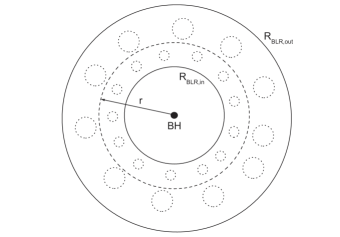
Figure 2: Sketch of axial cross section of the spherical geometry with some thickness and similar to Fig. 1 of Liu & Bai (2006).

3 APPLICATIONS

The new formulae are applied to broad-line radio galaxy 3C 120 at $z=0.033$ and blazar 3C 273 at redshift $z=0.158$, which were detected with Fermi-LAT.

3.1 Analysis of Time Lag

The z-transformed discrete correlation function (ZDCF; Alexander, 1997) is used to analyze cross-correlation. The centroid lag in cross-correlation function (CCF) is taken to characterize the time lag between broad-line and jet emission variations. The centroid time lag $\tau_{\rm{cent}}$ is computed by all the points with correlation coefficients not less than 0.8 times the maximum of correlation coefficients in the CCF bumps closer to the zero-lag (see Liu et al., 2011b). The model-independent flux randomization/random subset selection (FR/RSS) Monte Carlo method (Peterson et al., 1998b) is used to get the cross-correlation centroid distributions (CCCDs). The averages of CCCDs are taken as the time lags between the broad-line and jet emission variations, and the standard deviations of the same CCCDs are adopted as our formal $1\sigma$ uncertainties of these time lags. This treatment is same as in Grier et al. (2012) for the CCF analysis. Hereafter, $\tau_{\rm{cent}}$ equivalent to $\tau_{\rm{ob}}$.

3.2 3C 120

The 15 GHz light curve is published in Richards et al. (2011), and is obtained with a higher sampling of $\sim$ 60 times $\rm{yr^{-1}}$ by the OVRO 40 m blazar monitoring program. The H$\beta$ line light curves are from three different reverberation mapping monitoring works (Grier et al., 2012; Pozo Nuñez et al., 2012; Kollatschny et al., 2014). The data of Grier et al. (2012) and Pozo Nuñez et al. (2012) have a dense sampling of 20 times $\rm{month^{-1}}$. The data of Kollatschny et al. (2014) published currently have a rare sampling of 5 times $\rm{month^{-1}}$ and larger flux errors compared to the other two works. The data numbers and durations of light curves are presented in Table 1. These light curves are presented in Fig. 3. The combined H$\beta$ light curves of the three works are used to cross-correlate with the 15 GHz light curve. There is a positive time lag (see Figs. 4a and 4b and Table 2), which means the H$\beta$ line variations leading the 15 GHz variations. This new time lag is consistent with the previous result of $\tau_{\rm{cent}}=0.34\pm 0.01$ yr in Liu et al. (2014). For the H$\beta$ line, there are two outbursts, the outburst in Kollatschny et al. (2014) and the one in Grier et al. (2012), likely corresponding to the radio Outbursts I and II, respectively (see Fig. 3). The H$\gamma$ and He II $\lambda 4686$ outbursts in Kollatschny et al. (2014) likely correspond to Outburst I.

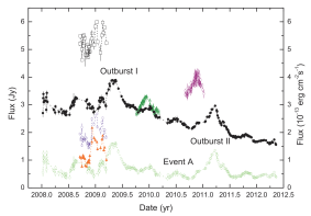
Figure 3: Light curves of broad-lines and 15 GHz emission. Olive triangles denote the H$\beta$ light curve of Pozo Nuñez et al. (2012). Purple circles denote the H$\beta$ light curve of Grier et al. (2012). Squares denote the H$\beta$ light curve of Kollatschny et al. (2014). Blue circles are the H$\gamma$ light curve of Kollatschny et al. (2014). Red triangles denote the He II $\lambda 4686$ light curve of Kollatschny et al. (2014). Black circles denote the 15 GHz light curve in units of Jy. The lines are in units of $10^{-13}\rm{\/\ erg\/\ cm^{-2}\/\ s^{-1}}$. Green circles are the 15 GHz light curve subtracted by an assumed simple baseline (Liu et al., 2014).

Figure 4: ZDCFs between the modified 15 GHz light curve and the broad-line light curves, and CCCDs obtained with the FR/RSS method in Monte Carlo simulations of 10,000 runs. (a) and (b) for the total H$\beta$ light curve. (c) and (d) for the He II $\lambda 4686$ light curve. (e) and (f) for the H$\gamma$ light curve.

Table 1: Fractional variability of 3C 120

Component	$F_{\rm{var}}$	$\sigma_{\rm{F_{\rm{var}}}}$	$N$	$D$ (yr)
(1)	(2)	(3)	(4)	(5)
H$\beta$ a	0.06	0.01	31	0.49
H$\beta$ b	0.057	0.005	102	0.42
H$\beta$ c	0.058	0.005	85	0.35
H$\beta$ d	0.23	0.01	218	1.26
H$\gamma$	0.18	0.02	31	0.49
He II $\lambda 4686$	0.30	0.04	31	0.49
15 GHz	0.22	0.01	257	4.34
Outburst I	0.34	0.04	45	0.66 †
Outburst II	0.27	0.04	31	0.59 †
Event A	0.15	0.03	27	0.46 †
H$\beta$ b	0.26	0.02	102	0.42 †
H$\beta$ c	0.21	0.02	85	0.35 †
H$\gamma$	0.31	0.04	31	0.49 †
He II $\lambda 4686$	0.30	0.04	31	0.49 †

Notes: Component: different components; $F_{\rm{var}}$: Fractional variability of light curves; $\sigma_{\rm{F_{\rm{var}}}}$: the error of $F_{\rm{var}}$; $N$: the observational data numbers in the light curves; $D$: the durations of light curves.

^a the H$\beta$ light curve in Kollatschny et al. (2014).

^b the H$\beta$ light curve in Pozo Nuñez et al. (2012).

^c the H$\beta$ light curve in Grier et al. (2012).

^d the total H$\beta$ light curve of three periods in notes a, b, and c.

^† the light curves denoted by the black solid and blue circles in Fig. 8.

The apparent speeds of the moving components with well-determined motions are all within a range of $\beta_{\rm{a}}=4.0\pm 0.2$ for 3C 120 (see Chatterjee et al., 2009). Grier et al. (2012) obtained a new size of $R_{\rm{BLR}}=27.2\pm 1.1$ light-days in their dense mapping observations for the H$\beta$ line. Pozo Nuñez et al. (2012) also obtained a new BLR size with small errors, which is consistent with that in Grier et al. (2012). This value of $R_{\rm{BLR}}=0.075\pm 0.003$ lt-yr is adopted here. The $1\sigma$ upper and lower limits of $R_{\rm{BLR}}$ are taken as $R_{\rm{BLR,out}}=0.078$ lt-yr and $R_{\rm{BLR,in}}=0.072$ lt-yr, respectively. The 43 GHz VLBA observations give the global parameters of the jet with a viewing angle $\alpha=20.5\pm 1.8^{\circ}$ for 3C 120 (Jorstad et al., 2005). For $\beta_{\rm{a}}=4.0\pm 0.2$, $\alpha=20.5\pm 1.8^{\circ}$, $\tau_{\rm{cent}}=0.35\pm 0.04$ yr, $R_{\rm{BLR,out}}=0.078$ and $R_{\rm{BLR,in}}=0.072$ lt-yr, we have $R_{\rm{jet}}=1.45\pm 0.02$ pc from Monte Carlo simulations based on equation (14) (see Table 2). This radio emitting region is at the pc-scale distance from the central engine.

Table 2: Estimated values of time lags $\tau_{\rm{cent}}$ and $R_{\rm{jet}}$ for 3C 120

Lines	$R_{\rm{BLR}}$ (lt-yr)	Ref.	$\tau_{\rm{cent}}$ (yr)	$R_{\rm{jet}}^{\rm{spher}}$ (pc)	$R_{\rm{jet}}^{\rm{disk}}$ (pc)	$R_{\rm{jet}}^{\rm{shell}}$ (pc)
(1)	(2)	(3)	(4)	(5)	(6)	(7)
H$\beta$	$0.075^{+0.003}_{-0.003}$	1	$0.35\pm 0.04$	$1.45\pm 0.02$	$1.45\pm 0.02$	$1.45\pm 0.02$
H$\gamma$	$0.065^{+0.013}_{-0.011}$	2	$0.29\pm 0.03$	$1.21\pm 0.01$	$1.21\pm 0.01$	$1.21\pm 0.02$
He II $\lambda 4686$	$0.033^{+0.021}_{-0.019}$	2	$0.31\pm 0.03$	$1.13\pm 0.01$	$1.14\pm 0.01$	$1.17\pm 0.03$

Notes: Lines: line names; $R_{\rm{BLR}}$: BLR sizes, $R_{\rm{BLR,in}}=R_{\rm{BLR}}-\sigma_{\rm{R_{\rm{BLR}}}}$ and $R_{\rm{BLR,out}}=R_{\rm{BLR}}+\sigma_{\rm{R_{\rm{BLR}}}}$ are taken to estimate $R_{\rm{jet}}$; Ref.: the references for column 2; $\tau_{\rm{cent}}$: Time lags, defined as $\tau_{\rm{cent}}=t_{\rm{radio}}-t_{\rm{line}}$, between broad-lines and radio emission; $R_{\rm{jet}}^{\rm{spher}}$: $R_{\rm{jet}}$ estimated with equation (14) for the spherical BLR; $R_{\rm{jet}}^{\rm{disk}}$: $R_{\rm{jet}}$ estimated with equation (19) for the disk-like BLR; $R_{\rm{jet}}^{\rm{shell}}$: $R_{\rm{jet}}$ estimated with equation (8) for the spherical shell or ring BLR.

References: (1) Grier et al. 2012; (2) Kollatschny et al. 2014.

In Kollatschny et al. (2014), the He II $\lambda 4686$ line was also monitored in the reverberation mapping observations, and this line light curve has a smaller flux errors than those in the H$\beta$ line light curve (see Fig. 3). The He II $\lambda 4686$ line light curve likely correspond to Outburst I in the 15 GHz light curve. The ZDCF method and the FR/RSS method show a positive time lag of the He II $\lambda 4686$ line relative to the 15 GHz variations (see Figs. 4c and 4d and Table 2). The H$\gamma$ line variations also seem to lead the 15 GHz variations by about 0.3 yr (see Fig. 3). Figs. 4e and 4f present the results from the ZDCF method and the FR/RSS method. There is a positive time lag around 0.3 yr (see Table 2 and Figs. 4e and 4f). These results indicate that the line variations lead the 15 GHz variations by about 0.3 yr, and confirm the positive lag from the H$\beta$ line. Kollatschny et al. (2014) estimated the sizes of the He II $\lambda 4686$ and H$\gamma$ lines, $R_{\rm{BLR}}=12.0^{+7.5}_{-7.0}$ and $R_{\rm{BLR}}=23.9^{+4.6}_{-3.9}$ light-days, respectively. Thus we have $R_{\rm{jet}}=1.13\pm 0.01$ and $1.21\pm 0.01$ pc from the He II $\lambda 4686$ and H$\gamma$ lines, respectively (see Table 2). The positions around one pc from the central engine are obtained from the time lags between these variations of the 15 GHz emission and the H$\beta$, H$\gamma$ and He II $\lambda 4686$ lines. These pc-scale distances from the central engine are larger than the BLR sizes by about two orders of magnitude. This indicates for 3C 120 that the gamma rays detected with Fermi-LAT are likely from the synchrotron-self Compton (SSC) processes in the jet if the gamma-ray emitting regions are around the radio emitting regions.

3.3 3C 273

From the 3C 273 database hosted by the ISDC (Türler et al., 1999) and updated by Soldi et al. (2008) (references therein), we take the 5, 8, 15, 22, and 37 GHz radio light curves. The sampling rates of 5, 8, 15, 22 and 37 GHz are 29, 40, 40, 44 and 46 times per year for the data considered, respectively. Only good data (Flag $>=$0) are used in the light curves considered here. Light curves of broad lines H$\alpha$, H$\beta$, and H$\gamma$ are from spectrophotometric reverberation mapping observations (Kaspi et al., 2000), and the sampling rates of the lines are around five times per year. Light curves of broad UV lines C iv $\lambda 1549$ and Ly$\alpha$ $\lambda 1216$ are from International Ultraviolet Explorer observations (Paltani & Türler, 2003). The sampling rates of the Ly$\alpha$ and C iv lines are around six times per year. The data numbers and durations of light curves are listed in Table 3. All the light curves are presented in Fig. 5.

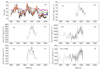
Figure 5: Light curves of 3C 273. (a) radio light curves: black color denotes 37 GHz light curve, red color 22 GHz one, blue color 15 GHz one, green color 8 GHz one, and magenta color 5 GHz one. (b) H$\alpha$ light curve. (c) H$\beta$ light curve. (d) H$\gamma$ light curve. (e) Ly$\alpha$ light curve. (f) C iv $\lambda 1549$ light curve.

Table 3: Fractional variability of 3C 273

Component	$F_{\rm{var}}$	$\sigma_{\rm{F_{\rm{var}}}}$	$N$	$D$ (yr)
(1)	(2)	(3)	(4)	(5)
H$\alpha$	0.08	0.01	34	7.13
H$\beta$	0.08	0.01	39	7.13
H$\gamma$	0.12	0.02	39	7.13
C iv $\lambda 1549$	0.12	0.01	119	17.79
Ly$\alpha$ $\lambda 1216$	0.11	0.01	119	17.79
5 GHz	0.072	0.002	784	26.90
8 GHz	0.143	0.003	1076	26.89
15 GHz	0.259	0.006	1063	26.88
22 GHz	0.286	0.006	1092	24.59
37 GHz	0.372	0.008	1247	26.67

Notes: Columns are same as Table 1.

The radio light curves after $\sim 1980$ are cross-correlated with the broad-line light curves. We performed 10,000 runs of Monte Carlo simulations, and the CCCDs are listed in Fig. 6. These time lags and uncertainties are listed in Table 4. All the CCCDs have a negative time lag (see Fig. 6), which indicates that the radio variations lead the broad-line variations. These CCCDs vary for different radio and broad-line light curves. The CCCDs between the H$\gamma$ line and radio variations seem to have similar profiles, and in general each of them is within a narrower interval. These similar and narrower CCCDs indicate good cross-correlations between the H$\gamma$ broad-line and radio jet emission variations.

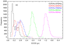
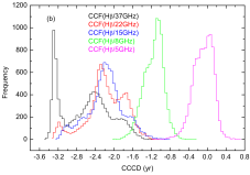
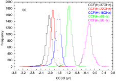
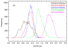
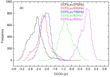
Figure 6: CCCDs obtained with the FR/RSS method in Monte Carlo simulations of 10,000 runs for 3C 273. (a) H$\alpha$ line, (b) H$\beta$ line, (c) H$\gamma$ line, (d) C iv $\lambda 1549$ line, and (e) Ly$\alpha$ line relative to radio emission variations.

Table 4: Time lags between broad-lines and radio emission for 3C 273

Lines	5 GHz	8 GHz	15 GHz	22 GHz	37 GHz
(1)	(2)	(3)	(4)	(5)	(6)
H$\alpha$	$-1.15\pm 0.15$	$-2.00\pm 0.14$	$-2.80\pm 0.18$	$-2.96\pm 0.21$	$-3.17\pm 0.17$
H$\beta$	$-0.09\pm 0.21$	$-1.15\pm 0.21$	$-2.18\pm 0.40$	$-2.18\pm 0.42$	$-2.60\pm 0.53$
H$\gamma$	$-0.28\pm 0.18$	$-1.15\pm 0.14$	$-1.66\pm 0.17$	$-1.87\pm 0.16$	$-2.05\pm 0.17$
C iv	$-0.54\pm 0.28$	$-1.35\pm 0.28$	$-2.11\pm 0.23$	$-2.21\pm 0.30$	$-2.53\pm 0.39$
Ly$\alpha$	$-0.14\pm 0.26$	$-1.04\pm 0.32$	$-2.05\pm 0.25$	$-2.16\pm 0.33$	$-2.52\pm 0.34$

Notes: Signs of time lags are defined as $\tau_{\rm{cent}}=t_{\rm{radio}}-t_{\rm{line}}$, in units of yr.

The broadband spectral energy distributions of 3C 273 constrain a Doppler factor $\delta=6.5$ (Ghisellini et al., 1998). These radio variations at high frequencies lead those of low frequencies (see Paper I). The time lags between the 5, 8, 15, 22, and 37 GHz variations can be explained by the radiation cooling effect of relativistic electrons with $\delta=6.5$ (see Fig. 6 in Paper I). The Doppler factor $\delta\geq 1.90$ is given by Xie et al. (2004) using the minimum timescale of variations at the optical band. The radiative cooling can match the time lags between these radio variations for $\delta=$3.5–6.5 (see Fig. 7). Thus we take $\delta=$3.5–6.5 with $\delta=\sqrt{1-\beta^{2}}/(1-\beta\cos\alpha)$ as a constraint in equations (8), (13), and (14). As in Paper I, we take $\alpha=12^{\circ}$–$21^{\circ}$ and $\beta=$0.9–0.995.

The sizes of BLRs for the Balmer lines are somehow controversial for 3C 273. Paltani & Türler (2005) think that the H$\alpha$, H$\beta$ and H$\gamma$ lags relative to the UV continuum are more reliable than those relative to the optical continuum. The UV continuum is more appropriate than the optical continuum as the ionizing continuum of the Balmer lines. The time lag of the H$\gamma$ line variations relative to the 37 GHz variations is $\tau_{\rm{ob}}=-2.05\pm 0.17$ yr (see Table 4). The H$\gamma$ line has a BLR size of $R_{\rm{BLR}}=2.85\pm 0.32$ lt-yr relative to the UV continuum (Paltani & Türler, 2005). Thus we get $R_{\rm{jet}}=8.63\pm 1.16$ lt-yr from Monte Carlo simulations based on equation (14) (see Table 5). This location of $R_{\rm{jet}}=2.65\pm 0.36$ pc is outside the BLR. Another possible choices of $R_{\rm{BLR}}$ and $\tau_{\rm{ob}}$ are the averages of the two quantities for the three Balmer lines. The average time lag is $\tau_{\rm{ob}}=-2.61\pm 0.17$ yr between the variations of the Balmer lines and the 37 GHz emission. The average BLR size is $R_{\rm{BLR}}=2.70\pm 0.13$ lt-yr for the Balmer lines relative to the UV continuum (Paltani & Türler, 2005). We have $R_{\rm{jet}}=3.27\pm 0.67$ lt-yr, i.e., $R_{\rm{jet}}=1.00\pm 0.21$ pc from the central engine. This position is around the BLR. These two estimated $R_{\rm{jet}}$ are at the pc-scale distance from the central engine, and the emitting regions on the pc-scales in the jet are difficult to be resolved in imaging observations.

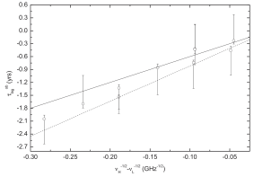
Figure 7: Same as Fig. 6 in Paper I. Time lags $\tau^{\rm{ob}}_{\rm{lag}}=t_{\rm{\nu_{H}}}-t_{\rm{\nu_{L}}}$ versus frequency differences $\nu^{-1/2}_{\rm{H}}-\nu^{-1/2}_{\rm{L}}$. Solid line is the expectation from the radiative cooling with $\delta=6.5$. Dashed line is for $\delta=3.5$.

4 Variability Amplitude

The root-mean-square fractional variability amplitude is used to measure the variability of a light curve, and the fractional variability amplitude $F_{\rm{var}}$ is (Rodriguez-Pascual et al., 1997)

$$F_{\rm{var}}=\sqrt{\frac{S^{2}-\langle\sigma^{2}_{\rm{err}}\rangle}{\langle F\rangle^{2}}},$$ (15)

where $\langle F\rangle$ is the mean flux, $S^{2}$ the variance, and $\langle\sigma^{2}_{\rm{err}}\rangle$ the measured mean square error. The error of $F_{\rm{var}}$ is (Edelson et al., 2002)

$$\sigma_{F_{\rm{var}}}=\frac{1}{F_{\rm{var}}}\sqrt{\frac{1}{2N}}\frac{S^{2}}{\langle F\rangle^{2}},$$ (16)

where $N$ is the number of data points in the light curve. $F_{\rm{var}}$ and $\sigma_{F_{\rm{var}}}$ are estimated for all the light curves for 3C 120 and 3C 273 (see Tables 1 and 3). For 3C 273, the broad lines and the 5 and 8 GHz emission have a comparable $F_{\rm{var}}$, i.e., a comparable variability. The 15, 22 and 37 GHz emission also have a comparable $F_{\rm{var}}$.

For 3C 120, the H$\beta$ line light curves have the same $F_{\rm{var}}$ at three periods. There are also comparable $F_{\rm{var}}$ for the H$\beta$ line total light curve, the H$\gamma$ line, the He II $\lambda 4686$ line, and the 15 GHz emission. Three components in the modified 15 GHz light curve are compared to the moved light curves of the H$\gamma$ and He II $\lambda 4686$ lines in Kollatschny et al. (2014), the H$\beta$ line in Grier et al. (2012), and the H$\beta$ line in Pozo Nuñez et al. (2012) (see Fig. 8). The H$\gamma$ and He II $\lambda 4686$ line light curves have similar profiles to Outburst I. There is a good correspondence between Outburst II and the H$\beta$ line light curve in Grier et al. (2012). Event A shows a correspondence to the H$\beta$ line light curve in Pozo Nuñez et al. (2012). Comparisons of the line light curves to Outbursts I and II and Event A show correspondences between the line and radio variations. The moved times in Fig. 8 are consistent with the time lags listed in Table 2, except for the H$\beta$ light curve and Event A, moved by 0.55 yr. This H$\beta$ light curve and Event A are at low states (see Fig. 3). Event A is likely produced by a weaker radio knot with a lower velocity, and the knot needs more times to travel from the central engine to the radio emitting region. Equation (8) shows that the time lag $\tau_{\rm{ob}}$ increases as the velocity $\beta_{\rm{a}}$ decreases if the radio emitting region is roughly around a position $R_{\rm{jet}}$. It is natural that the moved times of 0.55 yr for this H$\beta$ light curve and Event A is larger than the time lag of $\tau_{\rm{cent}}=0.35\pm 0.04$ yr for the total H$\beta$ light curve. Thus it should be reliable for 3C 120 that the line light curves correspond to Outbursts I and II and Event A presented in Fig. 8. The moved light curves of He II $\lambda 4686$ and H$\gamma$ lines have the same $F_{\rm{var}}$ consistent with that of Outburst I (see Table 1). Outburst II has a $F_{\rm{var}}$ consistent with that of the moved H$\beta$ light curve in Grier et al. (2012) (see Table 1). Event A has a $F_{\rm{var}}$ smaller than that of the moved H$\beta$ light curve in Pozo Nuñez et al. (2012) (see Table 1). These indicate that the variability amplitudes do not have inevitable relations with the correspondences (cross-correlations) between the broad-line and radio jet emission variations.

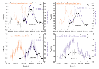
Figure 8: 3C 120: comparisons of 15 GHz components to the line light curves moved vertically and/or horizontally. The black solid circles are three components in the 15 GHz light curve, and the blue ones the moved line light curves.

5 DISCUSSION AND CONCLUSIONS

Another configuration of BLR is a disk-like structure (see e.g. Kollatschny et al., 2014; Pozo Nuñez et al., 2014). The disk-like BLR has a ratio of height to radius $C=H/r$. For a thin ring with a height $H$ in the range of $r\rightarrow r+dr$, it has a covering factor of $df_{\rm{cov}}(r)=n_{\rm{c}}(r)\sigma_{\rm{c}}(r)dr$ and a volume $dv=2\pi rHdr$. The emissivity of the thin ring within $r\rightarrow r+dr$ due to the photoionization of ultraviolet luminosity $L_{\rm{UV}}$ is

$$j_{\rm{BLR}}(r)=\frac{L_{\rm{UV}}df_{\rm{cov}}(r)}{4\pi dv}=\frac{L_{\rm{UV}}n_{\rm{c}}(r)\sigma_{\rm{c}}(r)}{8\pi^{2}Cr^{2}}\propto\frac{n_{\rm{c}}(r)\sigma_{\rm{c}}(r)}{r^{2}}.$$ (17)

Weighted averaging equation (8) over the whole BLR with the differential BLR flux within the range of $r\rightarrow r+dr$, and we have

$$R_{\rm{jet}}=\frac{\beta_{\rm{a}}}{\sin\alpha}\left(\frac{\int^{R_{\rm{BLR,out}}}_{R_{\rm{BLR,in}}}j_{\rm{BLR}}(r)rdr}{\int^{R_{\rm{BLR,out}}}_{R_{\rm{BLR,in}}}j_{\rm{BLR}}(r)dr}+\frac{\langle\tau_{\rm{ob}}\rangle}{1+z}c\right).$$ (18)

If $n_{\rm{c}}(r)$ and $\sigma_{\rm{c}}(r)$ have pow-law profiles, equation (18) will have the same expression as equation (13). For the disk-like BLR, the pow-law indexes $q$ and $p$ do not have the values similar to those derived from fitting the observed line light curves on the basis of photoionization calculations of a large number of clouds for the spherical BLR in Kaspi & Netzer (1999). Recently, Khajenabi (2015) investigated orbital motion of spherical, pressure-confined clouds in the BLR of AGNs, and found that a disk-like configuration is more plausible for the distribution of the BLR clouds. For a pressure-confined cloud, $r_{\rm{c}}(r)\varpropto P_{\rm{gas}}^{-1/3}$, where $P_{\rm{gas}}$ is the intercloud gas pressure and $P_{\rm{gas}}\varpropto r^{-5/2}$ (Khajenabi, 2015). Therefore, the cloud has a radius profile of $r_{\rm{c}}(r)\varpropto r^{5/6}$. This profile is similar to that one $r_{\rm{c}}(r)\varpropto r^{1/3}$ in Kaspi & Netzer (1999). A radial surface line emissivity profile of $F(r)\propto r^{-1}$ is assumed (in units of $\rm{erg\/\ s^{-1}\/\ cm^{-2}}$), and it is a fair approximation to the expected radial distribution derived from photoionization calculations for several of the commonly observed UV and optical emission lines (Goad et al., 2012). Thus, there is a differential broad-line flux $dF_{\rm{BLR}}(r)\varpropto r^{-2}dr$ in the range of $r\rightarrow r+dr$ for this profile. In the case of $dF_{\rm{BLR}}(r)\varpropto r^{-2}dr$, we have

$$\begin{split}R_{\rm{jet}}&=\frac{\beta_{\rm{a}}}{\sin\alpha}\left(\frac{\int^{R_{\rm{BLR,out}}}_{R_{\rm{BLR,in}}}rdF_{\rm{BLR}}(r)}{\int^{R_{\rm{BLR,out}}}_{R_{\rm{BLR,in}}}dF_{\rm{BLR}}(r)}+\frac{\langle\tau_{\rm{ob}}\rangle}{1+z}c\right)\\ &=\frac{\beta_{\rm{a}}}{\sin\alpha}\left(\frac{\int^{R_{\rm{BLR,out}}}_{R_{\rm{BLR,in}}}r^{-1}dr}{\int^{R_{\rm{BLR,out}}}_{R_{\rm{BLR,in}}}r^{-2}dr}+\frac{\langle\tau_{\rm{ob}}\rangle}{1+z}c\right)\\ &=\frac{\beta_{\rm{a}}}{\sin\alpha}\left(\frac{\ln R_{\rm{BLR,out}}-\ln R_{\rm{BLR,in}}}{R_{\rm{BLR,in}}^{-1}-R_{\rm{BLR,out}}^{-1}}+\frac{\langle\tau_{\rm{ob}}\rangle}{1+z}c\right).\end{split}$$ (19)

At the same time, $dF_{\rm{BLR}}(r)\varpropto j_{\rm{BLR}}(r)dr\varpropto n_{\rm{c}}(r)\sigma_{\rm{c}}(r)r^{-2}dr\varpropto r_{\rm{c}}^{2}r^{-p}r^{-2}dr=r^{5/3-p-2}dr$ ($r_{\rm{c}}(r)\varpropto r^{5/6}$). So, $p=5/3$ for the disk-like BLR. In the spherical BLR, $p=3/2$. The cloud number density profile of the spherical BLR is consistent with that of the disk-like BLR ($n_{\rm{c}}(r)\varpropto r^{-p}$ with comparable $p$ for the two kinds of BLRs).

The disk-like BLR geometry of 3C 120 has been established in Kollatschny et al. (2014) and Pozo Nuñez et al. (2014). Then $R_{\rm{jet}}$ will be re-calculated on the basis of equation (19). Based on $\tau_{\rm{cent}}$, $R_{\rm{BLR,in}}$ and $R_{\rm{BLR,out}}$ of the H$\beta$, H$\gamma$ and He II $\lambda 4686$ lines, $\beta_{\rm{a}}=4.0\pm 0.2$, $\alpha=20.5\pm 1.8^{\circ}$, and equation (19), averages of $R_{\rm{jet}}$ are derived from Monte Carlo simulations. These values of $R_{\rm{jet}}$ estimated under the disk-like BLR are consistent with those under the spherical BLR for 3C 120 (see Table 2). Equation (8) is based on a simple spherical shell or ring with a zero-thickness, and we also re-calculate $R_{\rm{jet}}$ with equation (8). The estimated results are presented in Table 2. These values are consistent with those estimated from equations (14) and (19). Therefore, the four BLRs with different configurations result in some negligible influences on $R_{\rm{jet}}$ for 3C 120. Modelling photometric reverberation data favors a nearly face-on disk-like BLR geometry with an inclination $i=10\pm 4^{\circ}$ and an extension from 22 to 28 light-days (Pozo Nuñez et al., 2014). If the viewing angle $\alpha=10\pm 4^{\circ}$ is adopted (and $R_{\rm{BLR}}$ spans from 22 to 28 light-days), $R_{\rm{jet}}$ is larger by a factor 2.0 than that value for $\alpha=20.5\pm 1.8^{\circ}$ and $R_{\rm{BLR}}=0.075\pm 0.003$ lt-yr. Thus the influence of the inclination of the disk-like BLR is more significant than that of the BLR configurations on $R_{\rm{jet}}$. This is also indicated by the dependence of $R_{\rm{jet}}$ on $\alpha$ scaling as $R_{\rm{jet}}\propto 1/\sin\alpha$. For the spherical BLR, the cloud density profile also has a $n_{\rm{c}}\propto r^{-p}$ with a possible value of $p=2$ (Kaspi & Netzer, 1999). $q=1/2$ or $q=1/3$ are possible values of the best models in Kaspi & Netzer (1999). Thus we consider the four combinations of $q=1/3,1/2$ and $p=3/2,2$ in equation (13) for 3C 273. The estimated values of $R_{\rm{jet}}$ are presented in Table 5. It is obvious that the different combinations of $q$ and $p$ only have weaker influences on $R_{\rm{jet}}$, and the influences are negligible for 3C 273.

Table 5: Influences of $q$ and $p$ on $R_{\rm{jet}}$ for 3C 273

Lines	$R_{\rm{BLR}}$ (lt-yr)	$\tau_{\rm{cent}}$(yr)	$R_{\rm{jet}}$ (pc)
			$\left(1/3,3/2\right)$	$\left(1/3,2\right)$	$\left(1/2,3/2\right)$	$\left(1/2,2\right)$
(1)	(2)	(3)	(4)	(5)	(6)	(7)
Balmer	$2.70^{+0.13}_{-0.13}$	$-2.61\pm 0.17$	$1.00\pm 0.21$	$1.00\pm 0.20$	$1.00\pm 0.21$	$1.00\pm 0.20$
H$\gamma$	$2.85^{+0.32}_{-0.32}$	$-2.05\pm 0.17$	$2.65\pm 0.36$	$2.63\pm 0.35$	$2.66\pm 0.36$	$2.64\pm 0.35$

Notes: Column 1: line names; Column 2: BLR sizes: $R_{\rm{BLR,in}}=R_{\rm{BLR}}-\sigma_{\rm{R_{\rm{BLR}}}}$ and $R_{\rm{BLR,out}}=R_{\rm{BLR}}+\sigma_{\rm{R_{\rm{BLR}}}}$; Column 3: Time lags defined as $\tau_{\rm{cent}}=t_{\rm{radio}}-t_{\rm{line}}$ between broad-lines and radio emission; Columns 4–7: $R_{\rm{jet}}$ estimated with equation (13) for different combinations of $(q,p)$. Balmer lines mean that $R_{\rm{BLR}}$ and $\tau_{\rm{cent}}$ are the averages of H$\alpha$, H$\beta$, and H$\gamma$ lines.

The emitting regions of radio outbursts are at the pc-scales from the central engines for 3C 120 and 3C 273 (see Tables 2 and 5). These regions may have an important impact on the gamma rays in 3C 120 and 3C 273, because that the gamma-ray emitting position relative to the BLR plays an important role in the gamma-ray emission from the jet (e.g. Sikora et al., 1994; Wang, 2000; Liu & Bai, 2006; Liu et al., 2008; Sitarek & Bednarek, 2008; Tavecchio & Ghisellini, 2008; Bai et al., 2009; Tavecchio & Mazin, 2009; Lei & Wang, 2014a). Recently, Max-Moerbeck et al. (2014) investigated the cross-correlations between these light curves of the brightest detected blazars from the first 3 years of the mission of Fermi-LAT and 4 years of 15 GHz observations from the OVRO 40 m monitoring program. They found for four sources that the radio variations lag the gamma-ray variations, suggesting that the gamma-ray emission originate upstream of the radio emission, i.e., $R_{\rm{\gamma}}\la R_{\rm{jet}}$. The constraint of $R_{\rm{\gamma}}\la R_{\rm{jet}}$ was also suggested in some researches (e.g. Dermer & Schlickeiser, 1994; Jorstad et al., 2001; Kovalev et al., 2009; Sikora et al., 2009; Abdo et al., 2010a). Thus, we have $R_{\rm{\gamma}}\la R_{\rm{jet}}\simeq$ 1.0–1.5 pc for 3C 120 and $R_{\rm{\gamma}}\la$1.0–2.6 pc for 3C 273. If we have known the relative sizes of $R_{\rm{jet}}$ to $R_{\rm{\gamma}}$ and $R_{\rm{BLR}}$, the relative size of $R_{\rm{\gamma}}$ to $R_{\rm{BLR}}$ would be constrained. The relative size of $R_{\rm{\gamma}}$ to $R_{\rm{BLR}}$ may be determined by a time lag between gamma-ray and broad-line variations if there is correlation. For 3C 120, $R_{\rm{jet}}\gg R_{\rm{BLR}}$, and then it is possible $R_{\rm{\gamma}}\gg R_{\rm{BLR}}$, which limits the EC component of gamma rays to be negligible compared to the SSC one. Tanaka et al. (2015) derived a ratio of EC to SSC luminosity of $\sim$ 0.1 for 3C 120. The dominant SSC component deduced here is consistent with Tanaka et al. (2015). For 3C 273, $R_{\rm{jet}}$ is slightly larger than $R_{\rm{BLR}}$. $R_{\rm{\gamma}}$ may be around or smaller than $R_{\rm{BLR}}$, and then the SSC component may be comparable to the EC one of gamma rays, i.e., the EC component is not negligible. In fact, the gamma-ray emitting position is complex relative to the BLR. For example, most of the time the gamma-ray emitting region is inside the BLR, but during some epoches the emitting region could drift outside the BLR. Foschini et al. (2011) proposed the very first idea, and recently Ghisellini et al. (2013) found a very clear case with multi-wavelength coverage. These will increase the complexity of the gamma-ray emission.

In this paper, we first derived a new formula under the spherical shell BLR with a zero thickness, and the formula connects $R_{\rm{jet}}$, $R_{\rm{BLR}}$, $\tau_{\rm{ob}}$, $\beta_{\rm{a}}$, and $\alpha$. The new formula is the same as that obtained under the ring BLR with a zero thickness (see Paper I). Second, we derived new formulae under the spherical BLR, a classical configuration, with cloud number density and radius radial profiles. The new formulae for the spherical BLR are applied to broad-line radio-loud Fermi-LAT AGNs 3C 120 and 3C 273. We analyzed the cross-correlations between broad-line and radio jet emission variations on the basis of the model-independent FR/RSS method and/or the ZDCF method. For 3C 120, a newly published paper presents H$\beta$, H$\gamma$ and He II $\lambda 4686$ line new data in reverberation mapping observations. Combined with the data sets of H$\beta$ line in other two papers, a longer light curve is used to cross-correlate with the 15 GHz light curve. The 15 GHz radio variations lag the broad-line H$\beta$, H$\gamma$ and He II $\lambda 4686$ variations, i.e., $\tau_{\rm{ob}}>0$, and $R_{\rm{jet}}\simeq$1.1–1.5 pc are estimated on the basis of the spherical BLR, the disk-like BLR, and the spherical shell and/or ring BLR (see Table 2). $R_{\rm{jet}}\gg R_{\rm{BLR}}$ for 3C 120, and this position far away from the central engine may have important influences on the gamma-ray emission. The radio variations lead the broad-line variations, i.e., $\tau_{\rm{ob}}<0$ for 3C 273. $R_{\rm{jet}}\simeq$1.0–2.6 pc are derived from the negative time lags for the spherical BLR. For 3C 273, $R_{\rm{jet}}\ga R_{\rm{BLR}}$, and we have $R_{\rm{\gamma}}\la R_{\rm{jet}}\simeq$ 1.0–2.6 pc. The gamma-ray flares detected with Fermi-LAT set a limit of $R_{\rm{\gamma}}<$ 1.6 pc for 3C 273 (Rani et al., 2013). The limit is marginally consistent with our constraint of $R_{\rm{\gamma}}\la$1.0–2.6 pc. This agreement indicates the reliability of the method used to estimate $R_{\rm{jet}}$. For 3C 120, $R_{\rm{\gamma}}\la R_{\rm{jet}}\simeq$ 1.0–1.5 pc. The cloud number density and radius radial profiles of the BLR have negligible influences on $R_{\rm{jet}}$ (see Table 5), and also the BLR configurations do (see Table 2). The inclination of the disk-like BLR will have a significant influence on $R_{\rm{jet}}$ (the viewing angle $\alpha$ is same as this inclination for the assumption that the jet axis is perpendicular to the plane of this BLR).

The black hole mass is of the order of $10^{7}M_{\rm{\odot}}$ in 3C 120 (Peterson et al., 1998a, 2004; Grier et al., 2012; Pozo Nuñez et al., 2012). Recently, Kollatschny et al. (2014) and Pozo Nuñez et al. (2014) derived larger masses of the order of $10^{8}M_{\rm{\odot}}$ for 3C 120. 3C 120 has $R_{\rm{jet}}=$1.1–1.5 pc and a mass of the order of $10^{8}M_{\rm{\odot}}$. 3C 273 has $R_{\rm{jet}}=$1.0–2.6 pc and a mass of the order of $10^{9}M_{\rm{\odot}}$ (Paltani & Türler, 2005). The radio emitting positions do not seem to scale with the masses of the central black holes for the two broad-line radio-loud Fermi-LAT AGNs. Until the moment there is no evidence that the positions of the emitting regions in the jets of AGNs scale with the masses of the central black holes, though this scaling relation (if present) will be important to the jet production and energy dissipation mechanisms in AGNs. Also, this scaling relation will be important with regard to jet-enhanced disk accretion in AGNs (Jolley & Kuncic, 2007a, b). In the future, the radio and gamma-ray emitting positions will be needed for more AGNs.

References

- Abdo et al. (2010a) Abdo, A. A., Ackermann, M., Ajello, M., et al. 2010a, Natur, 463, 919
- Abdo et al. (2010b) Abdo, A. A., Ackermann, M., Ajello, M., et al. 2010b, ApJ, 715, 429
- Abdo et al. (2010c) Abdo, A. A., Ackermann, M., Ajello, M., et al. 2010c, ApJ, 720, 912
- Ackermann et al. (2015) Ackermann, M., Ajello, M., Atwood, W., et al. 2015, arXiv: 1501.06054
- Alexander (1997) Alexander, T. 1997, in Astronomical Time Series, ed. D. Maoz, A. Sternberg, & E. M. Leibowitz (Dordrecht: Kluwer), 163
- Alexander & Netzer (1994) Alexander, T., & Netzer, H. 1994, MNRAS, 270, 781
- Alexander & Netzer (1997) Alexander, T., & Netzer, H. 1997, MNRAS, 284, 967
- Arshakian et al. (2010) Arshakian, T. G., León-Tavares, J., Lobanov, A. P., et al. 2010, MNRAS, 401, 1231
- Bai et al. (2009) Bai, J. M., Liu, H. T., & Ma, L. 2009, ApJ, 699, 2002
- Blandford & McKee (1982) Blandford, R. D., & McKee, C. F. 1982, ApJ, 255, 419
- Blandford & Payne (1982) Blandford, R. D., & Payne, D. G. 1982, MNRAS, 199, 883
- Blandford & Znajek (1977) Blandford, R. D., & Znajek, R. 1977, MNRAS, 179, 433
- Chatterjee et al. (2009) Chatterjee, R., Marscher, A. P., Jorstad, S. G., et al. 2009, ApJ, 704, 1689
- Chatterjee et al. (2011) Chatterjee, R., Marscher, A. P., Jorstad, S. G., et al. 2011, ApJ, 734, 43
- Dermer & Schlickeiser (1994) Dermer, C. D., & Schlickeiser, R. 1994, ApJS, 90, 945
- Edelson et al. (2002) Edelson, R., Turner, T. J., Pounds, K., et al. 2002, ApJ, 568, 610
- Foschini et al. (2011) Foschini, L., Ghisellini, G., Tavecchio, F., Bonnoli, G., & Stamerra, A. 2011, in Fermi Symposium Proceedings, ed. A. Morselli for the local organizing committee, eConf C110509 (http://www.slac.stanford.edu/econf/C110509/)
- Gaskell (2009) Gaskell, C. M. 2009, NewAR, 53, 140
- Goad et al. (2012) Goad, M. R., Korista, K. T., & Ruff, A. J. 2012, MNRAS, 426, 3086
- Ghisellini & Madau (1996) Ghisellini, G., & Madau, P. 1996, MNRAS, 280, 67
- Ghisellini et al. (1998) Ghisellini G., Celotti A., Fossati G., Maraschi L., & Comastri A. 1998, MNRAS, 301, 451
- Ghisellini et al. (2013) Ghisellini, G., Tavecchio, F., Foschini, L., Bonnoli, G., & Tagliaferri, G. 2013, MNRAS, 432, L66
- Grier et al. (2012) Grier, C. J., Peterson, B. M., Pogge, R. W., et al. 2012, ApJ, 755, 60
- Jolley & Kuncic (2007a) Jolley, E. J. D., Kuncic, Z. 2007a, Ap&SS, 310, 327
- Jolley & Kuncic (2007b) Jolley, E. J. D., Kuncic, Z. 2007b, Ap&SS, 311, 257
- Jorstad et al. (2001) Jorstad, S. G., Marscher, A. P., Mattox, J. R., et al. 2001, ApJ, 556, 738
- Jorstad et al. (2005) Jorstad, S. G., Marscher, A. P., Lister, M. L., et al. 2005, AJ, 130, 1418
- Kaspi & Netzer (1999) Kaspi, S., & Netzer, H. 1999, ApJ, 524, 71
- Kaspi et al. (2000) Kaspi, S., Smith, P. S., Netzer, H., et al. 2000, ApJ, 533, 631
- Kataoka et al. (2011) Kataoka, J., Stawarz, L., Takahashi, Y., et al. 2011, ApJ, 740, 29
- Khajenabi (2015) Khajenabi, F. 2015, MNRAS, 446, 1848
- Kollatschny et al. (2003) Kollatschny, W. 2003, A&A, 407, 461
- Kollatschny et al. (2014) Kollatschny, W., Ulbrich, K., Zetzl, M., Kaspi, S., & Haas, M. 2014, A&A, 566, A106
- Kovalev et al. (2009) Kovalev, Y. Y., Aller, H. D., Aller, M. F., et al. 2009, ApJL, 696, L17
- Lei & Wang (2014a) Lei, M. C., & Wang, J. C. 2014a, PASJ, 66, 7
- Lei & Wang (2014b) Lei, M. C., & Wang, J. C. 2014b, PASJ, 66, 92
- Liu & Bai (2006) Liu, H. T., & Bai, J. M. 2006, ApJ, 653, 1089
- Liu et al. (2008) Liu, H. T., Bai, J. M., & Ma, L. 2008, ApJ, 688, 148
- Liu et al. (2011a, hereafter Paper I) Liu, H. T., Bai, J. M., & Wang, J. M. 2011a, MNRAS, 414, 155 (Paper I)
- Liu et al. (2011b) Liu, H. T., Bai, J. M., Wang, J. M., & Li, S. K. 2011b, MNRAS, 418, 90
- Liu et al. (2014) Liu, H. T., Bai, J. M., Wang, J. M., & Li, S. K. 2014, AJ, 147, 17
- Marscher et al. (2002) Marscher, A. P., Jorstad, S. G., Gómez, J. L., et al. 2002, Natur, 417, 625
- Max-Moerbeck et al. (2014) Max-Moerbeck, W., Hovatta, T., Richards, J. L., et al. 2014, MNRAS, 445, 428
- Meier et al. (2001) Meier, D. L., Koide, S., & Uchida, Y. 2001, Sci, 291, 84
- Paltani & Türler (2003) Paltani S., & Türler M., 2003, ApJ, 583, 659
- Paltani & Türler (2005) Paltani S., & Türler M., 2005, A&A, 435, 811
- Penrose (1969) Penrose, R. 1969, NCimR, 1, 252
- Peterson et al. (2005) Peterson, B. M., Bentz, M. C., Desroches, L.-B., et al. 2005, ApJ, 632, 799
- Peterson et al. (2004) Peterson, B. M., Ferrarese, L., Gilbert, K. M., et al. 2004, ApJ, 613, 682
- Peterson et al. (1998a) Peterson, B. M., Wanders, I., Bertram, R., et al. 1998a, ApJ, 501, 82
- Peterson et al. (1998b) Peterson, B. M., Wanders, I., Horne, K., et al. 1998b, PASP, 110, 660
- Pozo Nuñez et al. (2012) Pozo Nuñez, F. P., Ramolla, M., Westhues, C., et al. 2012, A&A, 545, A84
- Pozo Nuñez et al. (2013) Pozo Nuñez, F., Westhues, C., Ramolla, M., et al. 2013, A&A, 552, A1
- Pozo Nuñez et al. (2014) Pozo Nuñez, F., Haas, M., Ramolla, M., et al. 2014, A&A, 568, A36
- Rani et al. (2013) Rani, B., Lott, B., Krichbaum, T. P., Fuhrmann, L., & Zensus, J. A. 2013, A&A, 557, 71
- Richards et al. (2011) Richards, J. L., Max-Moerbeck, W., Pavlidou, V., et al. 2011, ApJS, 194, 29
- Rodriguez-Pascual et al. (1997) Rodriguez-Pascual, P. M., Alloin, D., Clavel, J., et al. 1997, ApJS, 110, 9
- Sikora et al. (1994) Sikora, M., Begelman, M. C., & Rees, M. J. 1994, ApJ, 421, 153
- Sikora et al. (2009) Sikora, M., Stawarz, L., Moderski, R., Nalewajko, K., & Madejski, G. M. 2009, ApJ, 704, 38
- Sitarek & Bednarek (2008) Sitarek, J., & Bednarek, W. 2008, MNRAS, 391, 624
- Soldi et al. (2008) Soldi, S., Türler, M., Paltani, S., et al. 2008, A&A, 486, 411
- Tanaka et al. (2015) Tanaka, Y. T., Doi, A., Inoue, Y., et al. 2015, ApJL, 799, L18
- Tavecchio & Ghisellini (2008) Tavecchio, F., & Ghisellini, G. 2008, MNRAS, 386, 945
- Tavecchio & Mazin (2009) Tavecchio, F., & Mazin, D. 2009, MNRAS, 392, L40
- Türler et al. (1999) Türler M., Paltani, S., Courvoisier, T. J.-L., et al. 1999, A&AS, 134, 89
- Türler et al. (2000) Türler, M., Courvoisier, T. J.-L., & Paltani, S. 2000, A&A, 361, 850
- Wang (2000) Wang, J. M. 2000, ApJ, 538, 181
- Xie et al. (2004) Xie, G. Z., Zhou, S. B, & Liang, E. W. 2004, AJ, 127, 53
- Zhang (2013) Zhang, X. G. 2013, MNRAS, 431, L112