GPU-based acceleration of free energy calculations in solid state physics

Abstract

Obtaining a thermodynamically accurate phase diagram through numerical calculations is a computationally expensive problem that is crucially important to understanding the complex phenomena of solid state physics, such as superconductivity. In this work we show how this type of analysis can be significantly accelerated through the use of modern GPUs. We illustrate this with a concrete example of free energy calculation in multi-band iron-based superconductors, known to exhibit a superconducting state with oscillating order parameter (OP). Our approach can also be used for classical BCS-type superconductors. With a customized algorithm and compiler tuning we are able to achieve a 19x speedup compared to the CPU (119x compared to a single CPU core), reducing calculation time from minutes to mere seconds, enabling the analysis of larger systems and the elimination of finite size effects.

PROGRAM SUMMARY

Manuscript Title: GPU-based acceleration of free energy calculations in solid state physics
Authors: Michał Januszewski, Andrzej Ptok, Dawid Crivelli, Bartłomiej Gardas
Journal Reference:
Catalogue identifier:
Licensing provisions: LGPLv3
Programming language: Fortran, CUDA C
Computer: any with a CUDA-compliant GPU
Operating system: no limits (tested on Linux)
RAM: Typically tens of megabytes.
Keywords: superconductivity, FFLO, CUDA, OpenMP, OpenACC, free energy
Classification: 7, 6.5
Nature of problem: GPU-accelerated free energy calculations in multi-band iron-based superconductor models.
Solution method: Parallel parameter space search for a global minimum of free energy.
Unusual features:
The same core algorithm is implemented in Fortran with OpenMP and OpenACC compiler annotations, as well as in CUDA C. The original Fortran implementation targets the CPU architecture, while the CUDA C version is hand-optimized for modern GPUs.
Running time: problem-dependent, up to several seconds for a single value of momentum and a linear lattice size on the order of $10^{3}$.

1 Introduction

The last decade brought a dynamic evolution of the computing capabilities of graphics processing units (GPUs). In that time, the performance of a single card increased from tens of GFLOPS in NVxx to TFLOPS in the newest Kepler/Maxwell NVIDIA chips [1]. This raw processing power did not go unnoticed by the engineering and science communities, which started applying GPUs to accelerate a wide array of calculations in what became known as GPGPU – general-purpose computing on GPUs. This led to the development of special GPU variants optimized for high performance computing (e.g. the NVIDIA Tesla line), but it should be noted that even commodity graphics cards, such as those from the NVIDIA GeForce series, still provide enormous computational power and can be a very economical (both from the monetary and energy consumption point of view) alternative to large CPU clusters.

The spread of GPGPU techniques was further facilitated by the development of CUDA and OpenCL – parallel programming paradigms allowing efficient exploitation of the available GPU compute power without exposing the programmer to too many low-level details of the underlying hardware. GPUs were used successfully to accelerate many problems, e.g. the numerical solution of stochastic differential equations [4, 5], fluid simulations with the lattice Boltzmann method [2, 3], molecular dynamics simulations [6], classical [7] and quantum Monte Carlo [8] simulations, exact diagonalization of the Hubbard model  [9], etc.

Parallel computing in general, and its realization in GPUs in particular, can also be extremely useful in many fields of solid state physics. For a large number of problems, the ground state of the system and its free energy are of special interest. For instance, in order to determine the phase diagram of a model, free energy has to be calculated for a large number of points in the parameter space. In this paper, we address this very issue and illustrate it on a concrete example of a superconducting system with an oscillating order parameter (OP), specifically an iron-based multi-band superconductor (FeSC). Our algorithm is not limited to systems of this type and can also be used for systems in the homogeneous superconducting state (BCS).

The discovery of high temperature superconductivity in FeSC [10] began a period of intense experimental and theoretical research. [11] All FeSC include a two-dimensional structure which is shown in Fig. 1.a. The Fermi surfaces (FS) in FeSC are composed of hole-like Fermi pockets (around the $\Gamma=(0,0)$ point) and electron-like Fermi pockets (around the $M=(\pi,\pi)$ point) – Fig. 1.b. Moreover, in FeSC we expect the presence of $s_{\pm}$ symmetry of the superconducting OP. [12] In this case the OP exhibits a sign reversal between the hole pockets and electron pockets. For one $\mathtt{Fe}$ ion in the unit cell, the OP is proportional to $\cos k_{x}\cdot\cos k_{y}$.

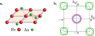
Figure 1: (Color on-line) (Panel a) $\mathtt{FeAs}$ layers in FeSC are built by $\mathtt{Fe}$ ions (red dots) forming a square lattice surrounded by $\mathtt{As}$ ions (green dots) which also form a square lattice. $\mathtt{As}$ ions are placed above or under the centers of the squares formed by $\mathtt{Fe}$. This leads to two inequivalent positions of $\mathtt{Fe}$ atoms, so that there are two ions of $\mathtt{Fe}$ and $\mathtt{As}$ in an elementary cell. (Panel b) True (folded) Fermi surface in the first Brillouin zone for two $\mathtt{Fe}$ ions in unit cell. The colors blue, red and green correspond to the FS for the 1st, 2nd, and 3rd band, respectively.

FeSC systems show complex low-energy band structures, which have been extensively studied. [12, 13, 14, 15, 16, 17] A consequence of this is a more sensitive dependence of the FS to doping. [18] In the superconducting state, the gap is found to be on the order of 10 meV, small relative to the breadth of the band. [19] This increases the required accuracy of calculated physical quantities needed to determine the phase diagram of the superconducting state, such as free energy. [20, 21]

In this paper we show how the increased computational cost of obtaining thermodynamically reliable results can be offset by parallelizing the most demanding routines using CUDA, after a suitable transformation of variables to decouple the interacting degrees of freedom. In Section 2 we discuss the theoretical background of numerical calculations. In Section 3 we describe the implementation of the algorithm and compare its performance when executed on the CPU and GPU. We summarize the results in Section 4.

2 Theoretical background

Many theoretical models of FeSC systems have been proposed, with two [22], three [23, 24, 25], four [26] and five bands [16, 17]. Most of the models mentioned describe one Fe unit cell and closely approximate the band and FS structure (Fig 1.b) obtained by LDA calculations. [15, 19, 27, 28] In every model the non-interacting tight-binding Hamiltonian of FeSC in momentum space can be described by:

$$H_{0}=\sum_{\alpha\beta{\bm{k}}\sigma}T^{\alpha\beta}_{{\bm{k}}\sigma}c_{\alpha{\bm{k}}\sigma}^{\dagger}c_{\beta{\bm{k}}\sigma},$$ (1)

where $c_{\alpha{\bm{k}}\sigma}^{\dagger}(c_{\alpha{\bm{k}}\sigma})$ is the creation (annihilation) operator for a spin $\sigma$ electron of momentum ${\bm{k}}$ in the orbital $\alpha$ (the set of orbitals is model dependent). The hopping matrix elements $T_{{\bm{k}}\sigma}^{\alpha\beta}=T_{\bm{k}}^{\alpha\beta}-\delta_{\alpha\beta}(\mu+\sigma h)$ determine the model of FeSC. Here, $\mu$ is the chemical potential and $h$ is an external magnetic field parallel to the FeAs layers. For our analysis we have chosen the minimal two-band model proposed by Raghu et al. [22] and the three-band model proposed by Daghofer et al. [23, 24] (described in A and B respectively). The band structure and FS of the FeSC system can be reconstructed by diagonalizing the Hamiltonian $H_{0}$:

$$H^{\prime}_{0} = \sum_{\varepsilon{\bm{k}}\sigma}E_{\varepsilon{\bm{k}}\sigma}d_{\varepsilon{\bm{k}}\sigma}^{\dagger}d_{\varepsilon{\bm{k}}\sigma},$$ (2)

where $d_{\varepsilon{\bm{k}}\sigma}^{\dagger}(d_{\varepsilon{\bm{k}}\sigma})$ is the creation (annihilation) operator for a spin $\sigma$ electron of momentum ${\bm{k}}$ in the band $\varepsilon$.

Superconductivity in multi-band iron-base systems in high magnetic fields

FeSC superconductors are layered [15, 19, 27, 28, 29, 30], clean [31, 32] materials with a relatively high Maki parameter $\alpha\sim 1-2$. [32, 33, 34, 35, 36] All of the features are shared with heavy fermion systems, in which strong indications exist to observe the Fulde–Ferrell–Larkin–Ovchinnikov (FFLO) phase [37, 38] – a superconducting phase with an oscillating order parameter in real space, caused by the non-zero value of the total momentum of Cooper pairs.

In contrast to the BCS state where Cooper pairs form a singlet state $({\bm{k}}\uparrow,-{\bm{k}}\downarrow)$, the FFLO phase is formed by pairing states $({\bm{k}}\uparrow,-{\bm{k}}+{\bm{q}}\downarrow)$. These states can occur between the Zeeman-split parts of the Fermi surface in a high external magnetic field (when the paramagnetic pair-breaking effects are smaller than the diamagnetic pair-breaking effects). [39] In one-band materials, the FFLO can be stabilized by anisotropies of the Fermi-surface and of the unconventional gap function, [40] by pair hopping interaction [41] or, in systems with nonstandard quasiparticles, with spin-dependent mass. [42, 43, 44, 45] This phase can be also realized in inhomogeneous systems in the presence of impurities [46, 47, 49] or spin density waves [50]. In some situations, the FFLO can be also stable in the absence of an external magnetic field. [51] In multi-band systems, the experimental [32, 33, 52, 53, 54] and theoretical [21, 55, 56, 57, 58, 59, 60] works point to the existence of the FFLO phase in FeSC. Through the analysis of the Cooper pair susceptibility in the minimal two-band model of FeSC, such systems are shown to support the existence of an FFLO phase, regardless of the exhibited OP symmetry. It should be noted that the state with nonzero Cooper pair momentum, in FeSC superconductors with the $s_{\pm}$ symmetry, is the ground state of the system near the Pauli limit. [21, 57] This holds true also for the three-band model (e.g. C and Ref. [60]).

Free energy for intra-band superconducting phase

In absence of inter-band interactions, the BCS and the FFLO phase (with Cooper pairs with total momentum ${\bm{q}}_{\varepsilon}$ equal zero and non-zero respectively) can be described by the effective Hamiltonian:

$$H_{SC}=\sum_{\varepsilon{\bm{k}}}\left(\Delta_{\varepsilon{\bm{k}}}d_{\varepsilon{\bm{k}}\uparrow}d_{\varepsilon,-{\bm{k}}+{\bm{q}}_{\varepsilon}\downarrow}+H.c.\right),$$ (3)

where $\Delta_{\varepsilon{\bm{k}}}=\Delta_{\varepsilon}\eta({\bm{k}})$ is the amplitude of the OP for Cooper pairs with total momentum ${\bm{q}}_{\varepsilon}$ (in band $\varepsilon$ with symmetry described by the form factor $\eta({\bm{k}})$ – for more details see Ref. [57]). Using the Bogoliubov transformation we can find the eigenvalues of the full Hamiltonian $H=H_{0}+H_{SC}$:

$$\mathcal{E}_{\varepsilon{\bm{k}}}^{\pm} = \frac{E_{\varepsilon{\bm{k}}\uparrow}-E_{\varepsilon,-{\bm{k}}+{\bm{q}}\downarrow}}{2}\pm\sqrt{\left(\frac{E_{\varepsilon{\bm{k}}\uparrow}+E_{\varepsilon,-{\bm{k}}+{\bm{q}}\downarrow}}{2}\right)^{2}+|\Delta_{\varepsilon{\bm{k}}}|^{2}}.$$ (4)

In this case we formally describe two independent bands. The total free energy for the system is given by $\Omega=\sum_{\varepsilon}\Omega_{\varepsilon}$, where

$$\Omega_{\varepsilon}=-\frac{1}{\beta}\sum_{\alpha\in\{+,-\}}\sum_{\bm{k}}\ln\left(1+\exp(-\beta\mathcal{E}_{\varepsilon{\bm{k}}}^{\alpha})\right)+\sum_{\bm{k}}\left(E_{\varepsilon{\bm{k}}\downarrow}-\frac{2|\Delta_{\varepsilon}|^{2}}{V_{\varepsilon}}\right),$$ (5)

corresponding to the free energy in $\varepsilon$-th band, where $V_{\varepsilon}$ is the respective interaction intensity and $\beta=1/k_{B}T$.

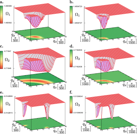
Figure 2: (Color on-line) Free energy $\Omega_{\varepsilon}$ for different parameters $V_{\varepsilon}$ in $h\simeq h_{C}^{BCS}$ – results for $h_{C}^{BCS}=0.025eV$ (panels a, c and e) and $0.005eV$ (panels b, d and f).

Historical and technical note

The historically basic concept of the FFLO phase was simultaneously proposed by two independent groups, Fulde-Ferrell [37] and Larkin-Ovchinnikov [38] in 1964. The first group proposed a superconducting phase where Cooper pairs have only one non-zero total momentum ${\bm{q}}$, and the superconducting order parameter in real space $\Delta({\bm{R}}_{j})\sim\exp(i{\bm{R}}_{j}\cdot{\bm{q}})$. In the second case, Cooper pairs have two possible momenta: ${\bm{q}}$ and the opposite $-{\bm{q}}$, with an equal amplitude of the order parameter. Thus in real space the superconducting order parameter is given by $\Delta({\bm{R}}_{j})\sim\exp(i{\bm{R}}_{j}\cdot{\bm{q}})+\exp(-i{\bm{R}}_{j}\cdot{\bm{q}})=\cos({\bm{R}}_{j}\cdot{\bm{q}})$. However, the most general case of FFLO is a superconducting order parameter given by a sum of plane waves, where the Cooper pairs have all compatible values of the momentum ${\bm{q}}_{\alpha}$ in the system:

$$\Delta(R_{j})=\sum_{\alpha=1}^{M}\Delta_{\alpha}\exp(i{\bm{R}}_{j}\cdot{\bm{q}}_{\alpha})$$ (6)

where $M$ is the cardinality of the first Brillouin zone (in the square lattice it is equal to $N_{x}\times N_{y}$). For the historical reasons described above, whenever $M=1$ (${\bm{q}}_{1}\neq 0$ and $\Delta_{1}\neq 0$) we can speak about the Fulde–Ferrell (FF) phase, whereas for $M=2$ (and ${\bm{q}}_{1}=-{\bm{q}}_{2}$, $\Delta_{1}=\Delta_{2}$) about the Larkin–Ovchinnikov (LO) phase.

Larger $M$ impose a more demanding spatial decomposition of the order parameter, both in the theoretical and computational sense. However, every time it can be reduced to the diagonalization of the (block) matrix representation of the Hamiltonian. Using the translational symmetry of the lattice, the problem for the FF phase ($M=1$) in one-band systems corresponds to the independent diagonalization of $2\times 2$ matrices (with eigenvalues given like in Eq. 4 with the number of bands $\varepsilon=1$) for each of the $N_{x}\times N_{y}$ different momentum sectors. In case of the LO phase ($M=2$), the calculation can be similarly decomposed in momentum space or using other spatial symmetries of the system (an example of this procedure can be found in Ref. [50]), with a much greater computational effort due to the lower degree of symmetry, leading to $N_{x}$ independent diagonalization problems of size $2N_{y}\times 2N_{y}$. In the full FFLO phase (i.e. in a system with impurities [46, 47, 49] or a vortex lattice [48]), the spatial decomposition is determined in real space using the self-consistent Bogoliubov-de Gennes equations, which require the full diagonalization of a Hamiltonian of maximal rank $2(N_{x}N_{y})$ [62, 63, 64, 65] at every self-consistent step. To work around these limitations, iterative methods [66, 67] or the Kernel Polynomial Method [68] can be used. These methods are based on the idea of expressing functions of the energy spectrum in an orthogonal basis, e.g. Chebyshev polynomial expansion. [69, 70, 71, 72, 73, 74, 75] By doing so, it becomes possible to conduct self-consistent calculations in the superconducting state without performing the diagonalization procedure. The time expense of iterative methods can also be reduced by a careful GPU implementation, which is currently a work in progress.

In the present work, we describe how the calculation of the free energy can be accelerated in the FF phase, which due to its greater symmetry allows optimal parallelization on a GPU architecture.

3 Parallel calculation of free energy

3.1 Programming models – OpenMP, OpenACC and CUDA C

Parallel programing can be realized in CPUs and GPUs in many different ways. In this section we compare the performance of the same algorithm implemented using OpenMP [80], PGI CUDA/OpenACC Fortran [79], and directly in CUDA C [1].

The first two are generic extensions of Fortran/C++ that make it easy to, respectively, use multiple CPU cores, and compile a subset of existing Fortran/C++ code for a GPU. They take the form of annotations which can be added to existing code, and as such, enable the use of additional computational power with very little overhead by the programmer. Typically, much better efficiency can be achieved by the third option – i.e. a specifically optimized implementation targeting the GPU architecture directly. This requires more work on the part of the programmer, both in adjusting the algorithms and in rewriting the code, but it makes it possible to fully utilize the available resources.

3.2 GPU algorithm

The global ground state for a fixed magnetic field strength $h$ and temperature $T$ is found by minimizing the free energy over the set of $\Delta_{\varepsilon}$ and ${\bm{q}}_{\varepsilon}$. In case of $n$ independent bands this corresponds to global minimization of the free energy $\Omega_{\varepsilon}$ in every band separately, for every ${\bm{q}}_{\varepsilon}$ in the first Brillouin zone (FBZ) – Algorithm 1.

For the calculation of the free energy $\Omega_{\varepsilon}$, we must know the eigenvalues $E_{\varepsilon{\bm{k}}\sigma}$ reconstructing the band structure of our systems. In the case of the two-band model, it can simply be found analytically (see A). However, for models with more bands (such as the three-band model – B) the band structure has to be determined numerically (e.g. using a linear algebra library, such as Lapack (CPU) or Magma (GPU) [77]). With this approach, the calculation of $E_{\varepsilon{\bm{k}}\uparrow}$ and $E_{\varepsilon,-{\bm{k}}+{\bm{q}}\downarrow}$ becomes a computationally costly procedure, and if it were to be repeated inside the inner loop of Algorithm 1, it would significantly impact the execution time. For this reason, we propose to precalculate the eigenvalues for every momentum vector ${\bm{k}}\in FBZ$ and store them in memory for models with more than two bands. The main downside of this approach is the large increase in memory usage.

While Algorithm 1 is simple to realize on a CPU, its execution time is proportional to the system size $N_{x}\times N_{y}$, and as such scales quadratically with $N_{x}$ for a square lattice ($N_{x}$ and $N_{y}$ are the number of lattice sites in the $x$ and $y$ direction, respectively).

Algorithm 1 Finding ${\bm{q}}_{\varepsilon}$ and $\Delta_{\varepsilon}$ corresponding to a global minimum of free energy in band $\varepsilon$.

1:  for ${\bm{q}}_{\varepsilon}\in FBZ$ do

2:     generate matrices $E_{\varepsilon{\bm{k}}\uparrow}$ and $E_{\varepsilon,-{\bm{k}}+{\bm{q}}_{i}\downarrow}$ for ${\bm{k}}\in FBZ$

3:     for $\Delta_{\varepsilon}=0$ to $\Delta_{max}$ do

4:        calculate matrices $\mathcal{E}_{\varepsilon{\bm{k}}}^{\pm}$ for ${\bm{k}}\in FBZ$ – Eq. 4

5:        calculate $\Omega_{\varepsilon}$

6:        find and save $\Delta_{\varepsilon}$ corresponding to a fixed ${\bm{q}}_{\varepsilon}$ and minimal value $\Omega_{\varepsilon}$

7:     end for

8:     find and save ${\bm{q}}_{\varepsilon}$ and $\Delta_{\varepsilon}$ corresponding to minimum of $\Omega_{\varepsilon}$

9:  end for

Sometimes the physical properties of the system make it possible to reduce the amount of computation – for instance when it is known that the minimum of the energy is attained for values of momentum ${\bm{q}}_{\varepsilon}$ in specific directions – Fig. 2. [21, 41, 49, 50, 57, 60, 61] In this case, the outer loop of Algorithm 1 can be restricted to ${\bm{q}}_{\varepsilon}\in\mathcal{Q}\subset FBZ$, where $\mathcal{Q}$ is a set of $N\ll N_{x}\times N_{y}$ vectors. Such reductions are not unique to linear systems with translational symmetry but are also the case for systems with rotational symmetry. [62, 63, 64]

In the case of BCS-type superconductivity where Cooper pairs have zero total momentum (${\bm{q}}_{\varepsilon}=0$), Algorithm 1 can be further simplified by taking into account the following property of the dispersion relation: $E_{\varepsilon,-{\bm{k}}}=E_{\varepsilon{\bm{k}}}$ in Eq. 4. This can be particularly useful in determining the system energy in the presence of the BCS phase – i.e. either in complete absence of external magnetic fields or when only weak fields are present.

A more general approach to the reduction of the execution time of our algorithm is to exploit the large degree of parallelism inherent in the problem. In fact, Algorithm 1 can be classified as ,,embarrassingly parallel” since the vast majority of computation can be carried out independently for all combinations of $\{{\bm{q}}_{\varepsilon},{\bm{k}},\Delta_{\varepsilon}\}$. For simplicity, in this paper we concentrate on optimizing the inner loop, as all the presented methods apply to the outer loop in a similar fashion.

We present two approaches to this problem. The first is to parallelize the execution of the serial loop over $\Delta_{\varepsilon}$ with OpenMP to fully utilize all available CPU cores. This has the advantage of simplicity, as the implementation requires minimal changes to the original (serial) code.

The second approach is to implement Algorithm 1 on a GPU using the CUDA environment. Modern GPUs are capable of simultaneously executing thousands of threads in SIMT (Same Instruction, Multiple Threads) mode. From a programmer’s point of view, all the threads are laid out in a 1-, 2- or 3-dimensional grid and are executing a kernel function. The grid is further subdivided into blocks (groups of threads), which are handled by a physical computational subunit of the GPU (the so-called streaming multiprocessor). Threads within a block can exchange data efficiently during execution, but cross-block communication can only take place through global GPU memory, which is significantly slower.

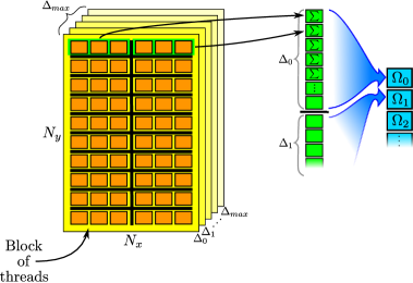
Figure 3: Schematic representation Algorithm 1 mapped to GPU hardware.

To fully utilize the GPU hardware, we split Algorithm 1 into three steps. In the first step, we execute the ComputeFreeEnergy kernel (Algorithm 2) on a 3D grid $N_{x}\times N_{y}\times\Delta_{max}$. To take advantage of the efficient intra-block communication, we also carry out partial sums within the block (corresponding to a subset of values spanning $N_{x}$) using the parallel sum-reduction algorithm. [78] In the second step, we execute the sum-reduction algorithm again on the partial sums that were generated by Algorithm 2. In the third and last step, we copy the output of step 2 from GPU memory to host memory, and look for the value of $\Delta_{i}$ corresponding to the lowest free energy with a linear search. Depending on the exact configuration of the kernels in step 1 and 2, the summation might not be complete at the beginning of step 3. If this is the case, we carry out the remaining summation within the serial loop computing $\Delta_{i}$. With block sizes of 128 and 1024 used for the kernels in steps 1 and 2, we can sum up to $2^{17}$ terms in parallel on the GPU. We found that the remaining summation was not worth the overhead of carrying it out on the GPU. Should this not be the case for some larger problems, further parallel execution can be trivially achieved by repeating step 2 one more time.

Algorithm 2 The ComputeFreeEnergy CUDA kernel.

1:  compute $\Delta_{i}$ and ${\bm{k}}$ corresponding to the current thread

2:  load $E_{i{\bm{k}}\uparrow}$ and $E_{i,-{\bm{k}}+{\bm{q}}_{\varepsilon}\downarrow}$ from global memory (precomputed by a separate kernel)

3:  compute $\mathcal{E}_{i{\bm{k}}}^{\pm}$ and $\Omega_{i}$

4:  sum $\Omega_{i}$ for a range of ${\bm{k}}$ corresponding to one block of threads

5:  save the partial sum from the previous step in global GPU memory

3.3 Performance evaluation

To test our approach, we executed Algorithms 1 and 2 on Linux machines with the following hardware:

• CPU: Intel(R) Core(TM) i7-3960X CPU @ 3.30GHz – 6 cores / 12 threads,

• GPU: NVIDIA Tesla K40 (GK180) with the SM clock set to 875 MHz.

The programs were run for a single value of ${\bm{q}}_{i}$ and 200 values of $\Delta_{i}$. Calculations were done for a square lattice of size $N\times N$ for various values of $N$. The execution times (including only the computation part of the code, and excluding any time spent on startup or input/output) are presented in Figure 4.

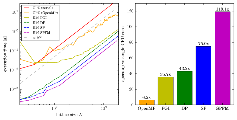
Figure 4: (Color on-line) Left panel: Execution time of Algorithm 1 and 2 for one vector ${\bm{q}}_{i}$. Right panel: speedup factors for all configurations at $N=2000$. The last 3 case names correspond to runs of the same CUDA C code in double precision (DP), single precision (SP), and single precision with fast intrinsic functions (SPFM). All versions of the Fortran code used double precision calculations.

Comparing the best CPU execution time (with OpenMP) to the GPU Fortran code using OpenACC, we find a speedup factor of $5.8$ in the limit of large lattices. The custom GPU code shows slightly better performance, with a $7$x speedup for the double precision version, and additional speedup factors of $1.7$ for single precision, and $1.6$ for intrinsic functions. When taken together, the fastest GPU version is $19.2$ times faster than the OpenMP code and $119.1$ times faster than the serial CPU code utilizing only a single core.

It is remarkable that the original Fortran code enhanced with OpenACC annotations provides performance comparable to a manual implementation in CUDA C. This result shows the power of appropriately used annotations marking parallelizable regions of the code. While still requiring explicit input from the programmer and a good understanding of the structure of the code, this approach is in practice significantly faster than writing the program from scratch in CUDA C and dealing with low level details of GPU programming and resource allocation. This conclusion however only applies in the limit of large lattices (see the left panel in Figure 4). For smaller ones, the CUDA C code can be seen to be noticeably faster than OpenACC, which is likely caused by the automatically generated GPU code introducing unnecessary overhead.

It should be noted that the last two speedup factors were achieved by trading off precision of calculations for performance – e.g. intrinsic functions are faster, but less precise implementations of transcendental functions. In our tests, we obtained the same results with all three approaches. This might not be true for some other systems though, so we advise careful experimentation. With a factor of 2.8x between the most and least precise method, it might also be worthwhile to run larger parameter scans at lower precision and then selectively verify with double precision calculations.

4 Summary

The rich phenomenology and the subtle competing and interplaying phenomena of high-$T_{C}$ materials such as FeSC (Section 1), require us to probe fine regimes and precisely determine possible experimental signatures of exotic phases such as FFLO (Section 2).

By conducting our calculations in momentum space, and by fully exploiting the symmetries of the system, we are able to increase the size of the studied system by two orders of magnitude compared to previously reported results and practically eliminate finite size effects. The cost is borne by the increased complexity of the efficient custom-tailored GPU implementation, described in Section 3. Our method shown here on the example of an iron-based multi-band superconductor exhibiting a FFLO phase, can also be used in calculations of the ground state in standard BCS-type superconductors.

Overall, we achieved a 19x speedup compared to the CPU implementation (119x compared a single CPU core). In the spectrum of GPU-accelerated results in physics, this puts us towards the higher end, with the highest speedups being $\approx 700$x for compute-bound problems with large inherent parallelism. [4]

Appendix A Two-band model of Raghu et al.

The model of FeSC proposed by Raghu et al. in Ref. [22], is a minimal two-band model of iron-base pnictides describing the $d_{xz}$ and $d_{yz}$ orbitals with hybridization:

$$T_{\bm{k}}^{11} = -2\left(t_{1}\cos k_{x}+t_{2}\cos k_{y}\right)-4t_{3}\cos k_{x}\cos k_{y}$$ (7)

$$T_{\bm{k}}^{22} = -2\left(t_{2}\cos k_{x}+t_{1}\cos k_{y}\right)-4t_{3}\cos k_{x}\cos k_{y}$$ (8)

$$T_{\bm{k}}^{12} = T_{\bm{k}}^{21}=-4t_{4}\sin k_{x}\sin k_{y},$$ (9)

where $t_{1}=-1.0$, $t_{2}=1.3$, $t_{3}=-0.85$, $t_{4}=-0.85$. $|t_{1}|$ is the energy unit. Half-filling, a configuration with two electrons per site requires $\mu=1.54|t_{1}|$. The model is exactly diagonalizable, with eigenvalues:

$$E_{\pm,{\bm{k}}}=\frac{T_{\bm{k}}^{11}+T_{\bm{k}}^{22}}{2}\pm\sqrt{\left(\frac{T_{\bm{k}}^{11}-T_{\bm{k}}^{22}}{2}\right)^{2}+(T_{\bm{k}}^{12})^{2}}.$$ (10)

The spectrum $E_{\alpha{\bm{k}}}$ reproduces the band structure and Fermi surface of FeSC – for $\alpha=+(-)$ we get the electron-like (hole-like) band.

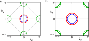
Figure 5: (Color on-line) Unfolded 1Fe/cell (panel a) and folded 2Fe/cell (panel b.) Fermi surface for the three-band model of pnictides proposed by Daghofer et al. in Ref. [24]. The dashed gray line in panel a. shows the true Brillouin zone. The colors blue, red and green correspond to the FS for the 1st, 2nd, and 3rd band, respectively.

Appendix B Three-band model Daghofer et al.

This model of FeSC was proposed by Daghofer et al. in Ref. [23] and improved in Ref. [24]. Beyond the $d_{xz}$ and $d_{yz}$ orbitals, the model also accounts for the $d_{xy}$ orbital:

$$T_{\bm{k}}^{11} = 2t_{2}\cos k_{x}+2t_{1}\cos k_{y}+4t_{3}\cos k_{x}\cos k_{y}$$

$$+ 2t_{11}(\cos(2k_{x})-\cos(2k_{y}))+4t_{12}\cos(2k_{x})\cos(2k_{y}),$$

$$T_{\bm{k}}^{22} = 2t_{1}\cos k_{x}+2t_{2}\cos k_{y}+4t_{3}\cos k_{x}\cos k_{y}$$

$$- 2t_{11}(\cos(2k_{x})-\cos(2k_{y}))+4t_{12}\cos(2k_{x})\cos(2k_{y}),$$

$$T_{\bm{k}}^{33} = \epsilon_{0}+2t_{5}(\cos k_{x}+\cos k_{y})+4t_{6}\cos k_{x}\cos k_{y}$$

$$+ 2t_{9}(\cos(2k_{x})+\cos(2k_{y}))$$

$$+ 4t_{10}(\cos(2k_{x})\cos k_{y}+\cos k_{x}\cos(2k_{y})),$$

$$T_{\bm{k}}^{12} = T_{\bm{k}}^{21}=4t_{4}\sin k_{x}\sin k_{y},$$ (14)

$$T_{\bm{k}}^{13} = \bar{T}_{\bm{k}}^{31}=2it_{7}\sin k_{x}+4it_{8}\sin k_{x}\cos k_{y},$$ (15)

$$T_{\bm{k}}^{23} = \bar{T}_{\bm{k}}^{32}=2it_{7}\sin k_{y}+4it_{8}\sin k_{y}\cos k_{x}.$$ (16)

In Ref. [24] the hopping parameters in electron volts are given as: $t_{1}=-0.08$, $t_{2}=0.1825$, $t_{3}=0.08375$, $t_{4}=-0.03$, $t_{5}=0.15$, $t_{6}=0.15$, $t_{7}=-0.12$, $t_{8}=0.06$, $t_{9}=0.0$, $t_{10}=-0.024$, $t_{11}=-0.01$, $t_{12}=0.0275$ and $\epsilon_{0}=0.75$. The average number of particles in the system $n=4$ is attained for $\mu=0.4748$. The FS for this model is shown in Fig. 5.

Appendix C The static Cooper pair susceptibility in the three-band model

The static Cooper pair susceptibility indicates the possible formation of the FFLO phase: [57, 61]

$$\chi_{\varepsilon\varepsilon^{\prime}}^{\Delta}({\bm{q}}) \equiv \lim_{\omega\rightarrow 0}-\frac{1}{N}\sum_{{\bm{i}}{\bm{j}}}\exp(i{\bm{q}}\cdot({\bm{i}}-{\bm{j}}))\langle\langle\widehat{\Delta}_{\varepsilon\varepsilon^{\prime}{\bm{i}}}|\widehat{\Delta}_{\varepsilon\varepsilon^{\prime}{\bm{j}}}^{\dagger}\rangle\rangle^{r},$$ (17)

where $\langle\langle.|.\rangle\rangle^{r}$ is the retarded Green’s function and $\widehat{\Delta}_{\varepsilon{\bm{i}}}=\sum_{\bm{j}}\vartheta({\bm{j}}-{\bm{i}})d_{\varepsilon{\bm{i}}\uparrow}d_{\varepsilon{\bm{j}}\downarrow}$ is the OP in band $\varepsilon$. The operator $d_{\varepsilon{\bm{i}}\sigma}$ in real space corresponds to the operator $d_{\varepsilon{\bm{k}}\sigma}$ in momentum space. The factor $\vartheta({\bm{j}}-{\bm{i}})$ defines the OP symmetries – for $s_{\pm}$ pairing, $\vartheta({\bm{\delta}})$ is equal to $1$ for next nearest neighbors and zero otherwise. [57] In momentum space:

$$\chi_{\varepsilon\varepsilon^{\prime}}^{\Delta}({\bm{q}})=\lim_{\omega\rightarrow 0}-\frac{1}{N}\sum_{{\bm{k}}{\bm{l}}}\eta(-{\bm{k}}-{\bm{q}})\eta(-{\bm{l}}-{\bm{q}})\mathcal{G}_{\varepsilon\varepsilon^{\prime}}({\bm{k}},{\bm{l}},{\bm{q}},\omega),$$ (18)

$$\mathcal{G}_{\varepsilon\varepsilon^{\prime}}({\bm{k}},{\bm{l}},{\bm{q}},\omega) = \langle\langle d_{\varepsilon{\bm{k}}\uparrow}d_{\varepsilon^{\prime},-{\bm{k}}-{\bm{q}}\downarrow}|d_{\varepsilon^{\prime},-{\bm{l}}-{\bm{q}}\downarrow}^{\dagger}d_{\varepsilon{\bm{l}}\uparrow}^{\dagger}\rangle\rangle^{r}$$ (19)

$$= \delta_{{\bm{k}}{\bm{l}}}\frac{f(-E_{\varepsilon{\bm{k}}\uparrow})-f(E_{\varepsilon^{\prime},-{\bm{k}}-{\bm{q}}\downarrow})}{\omega-E_{\varepsilon{\bm{k}}\uparrow}-E_{\varepsilon^{\prime},-{\bm{k}}-{\bm{q}}\downarrow}}$$

where $\eta({\bm{k}})=4\cos(k_{x})\cos(k_{y})$ is the structure factor corresponding to the $s_{\pm}$-wave symmetry, and $f$ is the Fermi function. This quantity can be calculated numerically similarly to the procedure used for free energy in Section 2.

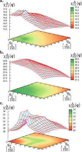
Figure 6: (Color on-line) The static Cooper pair susceptibility $\chi^{\Delta}_{\varepsilon\varepsilon^{\prime}}$ in magnetic field $h=0.025$ eV and temperature $k_{B}T\simeq 0$ eV.

References

- [1] NVIDIA Corporation, CDUA C Programming Guide, version 5.5 (2013)
- [2] J. Tölke, M. Krafczyk, TeraFLOP computing on a desktop PC with GPUs for 3D CFD, International Journal of Computational Fluid Dynamics 22 (2008) 443
- [3] M. Januszewski, M. Kostur, Sailfish: A flexible multi-GPU implementation of the lattice Boltzmann method, Comput. Phys. Commun. (2014)
- [4] M. Januszewski, M. Kostur, Accelerating numerical solution of Stochastic Differential Equations with CUDA, Comput. Phys. Commun. 181 (2010) 183
- [5] J. Spiechowicz, M. Kostur, L. Machura, GPU accelerated Monte Carlo simulation of Brownian motors dynamics with CUDA, Comput. Phys. Commun., accepted, 2015
- [6] J. A. Anderson, C. D. Lorenz, A. Travesset, General purpose molecular dynamics simulations fully implemented on graphics processing units, J. Comput. Phys. 227 (2008) 5342
- [7] T. Preis, P. Virnau, P. Wolfgang and J. J. Schneider, GPU accelerated Monte Carlo simulation of the 2D and 3D Ising model, J. Comput. Phys. 228 (2009) 4468
- [8] A. G. Andersona, W. A. Goddard III, P. Schröderb, Quantum Monte Carlo on graphical processing units, Comput. Phys. Commun. 177 (2007) 298
- [9] T. Siro and A. Harju, Exact diagonalization of the Hubbard model on graphics processing units, Comput. Phys. Commun. 183 (2012) 1884
- [10] Y. Kamihara, T. Watanabe, M. Hirano, H. Hosono, Iron-Based Layered Superconductor (x = 0.05-0.12) with = 26 K, J. Am. Chem. Soc. 130 (2008) 3296
- [11] K. Ishida, Y. Nakai, H. Hosono, To What Extent Iron-Pnictide New Superconductors Have Been Clarified: A Progress Report, J. Phys. Soc. Jpn. 78 (2009) 062001
- [12] I.I. Mazin, D.J. Singh, M.D. Johannes, M.H. Du, Unconventional Superconductivity with a Sign Reversal in the Order Parameter of , Phys. Rev. Lett. 101 (2008) 057003
- [13] J. Kunes, R. Arita, P. Wissgott, A. Toschi, H. Ikeda, K. Held, Wien2wannier: From linearized augmented plane waves to maximally localized Wannier functions, Comput. Phys. Commun. 181 (2010) 1888
- [14] L. Boeri, O. V. Dolgov, A. A. Golubov, Is an Electron-Phonon Superconductor?, Phys. Rev. Lett. 101 (2008) 026403
- [15] D. J. Singh, M.-H. Du, Density Functional Study of : A Low Carrier Density Superconductor Near Itinerant Magnetism, Phys. Rev. Lett. 100 (2008) 237003
- [16] S. Graser, T. A. Maier, P. J. Hirschfeld, D. J. Scalapino, Near-degeneracy of several pairing channels in multiorbital models for the Fe pnictides, New J. Phys. 11 (2009) 025016
- [17] K. Kuroki, S. Onari, R. Arita, H. Usui, Y. Tanaka, H. Kontani, H. Aoki, Unconventional Pairing Originating from the Disconnected Fermi Surfaces of Superconducting , Phys. Rev. Lett. 101 (2008) 087004
- [18] L. Pan, J. Li, Y. Y. Tai, M. J. Graf, J. X. Zhu, C. S. Ting, Evolution of the Fermi surface topology in doped 122 iron pnictides, Phys. Rev. B 88 (2013) 214510
- [19] H. Ding, P. Richard, K. Nakayama, K. Sugawara, T. Arakane, Y. Sekiba, A. Takayama, S. Souma, T. Sato, T. Takahashi, Z. Wang, X. Dai, Z. Fang, G. F. Chen, J. L. Luo, N. L. Wang, Observation of Fermi-surface–dependent nodeless superconducting gaps in , Europhys. Lett. 83 (2008) 47001
- [20] Y. Y. Tai, J. X Zhu, M. J. Graf, C. S. Ting, Calculated phase diagram of doped BaFe2As2 superconductor in a C4-symmetry breaking model, Europhys. Lett. 103 (2013) 67001
- [21] A. Ptok, Influence of symmetry on unconventional superconductivity in pnictides above the Pauli limit – two-band model study, Eur. Phys. J. B 87 (2014) 2
- [22] S. Raghu, X. L. Qi, C. X. Liu, D. J. Scalapino, S. C. Zhang, Minimal two-band model of the superconducting iron oxypnictides, Phys. Rev. B 77 (2008) 220503(R)
- [23] M. Daghofer, A. Nicholson, A. Moreo, E. Dagotto, Three orbital model for the iron-based superconductors, Phys. Rev. B 81 (2010) 014511
- [24] M. Daghofer, A. Nicholson and A. Moreo, Spectral density in a nematic state of iron pnictides, Phys. Rev. B 85 (2012) 184515
- [25] M. M. Korshunov, Y. N. Togushova, I. Eremin, Spin-Orbit Coupling in Fe-Based Superconductors, J. Supercond. Nov. Magn. 26 (2013) 2665
- [26] M. M. Korshunov, I. Eremin,Theory of magnetic excitations in iron-based layered superconductors, Phys. Rev. B 78 (2008) 140509(R)
- [27] T. Kondo, A. F. Santander-Syro, O. Copie, C. Liu, M. E. Tillman, E. D. Mun, J. Schmalian, S. L. Bud’ko, M. A. Tanatar, P. C. Canfield, A. Kaminski, Momentum Dependence of the Superconducting Gap in Single Crystals Measured by Angle Resolved Photoemission Spectroscopy, Phys. Rev. Lett. 101 (2008) 147003
- [28] V. Cvetkovic, Z. Tesanovic, Valley density-wave and multiband superconductivity in iron-based pnictide superconductors, Phys. Rev. B 80 (2009) 024512
- [29] C. Liua, T. Kondoa, A.D. Palczewskia, G.D. Samolyuka, Y. Leea, M.E. Tillmana, Ni Nia, E.D. Muna, R. Gordona, A.F. Santander-Syrob, c, S.L. Budḱoa, J.L. McChesneyd, E. Rotenbergd, A.V. Fedorovd, T. Vallae, O. Copief, M.A. Tanatara, C. Martina, B.N. Harmona, P.C. Canfielda, R. Prozorova, J. Schmaliana, A. Kaminskia, Electronic properties of iron arsenic high temperature superconductors revealed by angle resolved photoemission spectroscopy (ARPES), Physica C 469 (2009) 491
- [30] V. Cvetkovic, Z. Tesanovic, Multiband magnetism and superconductivity in Fe-based compounds, Europhys. Lett. 85, (2009) 37002
- [31] H. Kim, M. A. Tanatar, Y. J. Song, Y. S. Kwon, R. Prozorov, Nodeless two-gap superconducting state in single crystals of the stoichiometric iron pnictide LiFeAs, Phys. Rev. B 83 (2011) 100502(R)
- [32] S. Khim, B. Lee, J.W. Kim, E.S. Choi, G.R. Stewart, K.H. Kim, Pauli-limiting effects in the upper critical fields of a clean LiFeAs single crystal, Phys. Rev. B 84 (2011) 104502
- [33] K. Cho, H. Kim, M.A. Tanatar, Y.J. Song, Y.S. Kwon, W.A. Coniglio, C.C. Agosta, A. Gurevich, R. Prozorov, Anisotropic upper critical field and possible Fulde-Ferrel-Larkin-Ovchinnikov state in the stoichiometric pnictide superconductor LiFeAs, Phys. Rev. B 83 (2011) 060502(R)
- [34] J. L. Zhang, L. Jiao, F. F. Balakirev, X. C. Wang, C. Q. Jin, and H. Q. Yuan, Upper critical field and its anisotropy in LiFeAs, Phys. Rev. B 83 (2011) 174506
- [35] N. Kurita, K. Kitagawa, K. Matsubayashi, A. Kismarahardja, E.-S. Choi, J. S. Brooks, Y. Uwatoko, S. Uji, T. Terashima, Determination of the Upper Critical Field of a Single Crystal LiFeAs: The Magnetic Torque Study up to 35 Tesla, J. Phys. Soc. Jpn. 80 (2011) 013706
- [36] T. Terashima, K. Kihou, M. Tomita, S. Tsuchiya, N. Kikugawa, S. Ishida, C.-H. Lee, A. Iyo, H. Eisaki, S. Uji, First-order superconducting resistive transition in , Phys. Rev. B 87 (2013) 184513
- [37] P. Fulde, R. A. Ferrel, Superconductivity in a Strong Spin-Exchange Field, Phys. Rev. 135 (1964) A550
- [38] A. I. Larkin, Yu. N.Ovchinnikov, Inhomogeneous State of Superconductors, Zh. Eksp. Teor. Fiz.47 (1964) 1136, [Sov. Phys. JETP 20 (1965) 762]
- [39] Y. Matsuda, H. Shimahara, Fulde-Ferrell-Larkin-Ovchinnikov State in Heavy Fermion Superconductors, J. Phys. Soc. Jpn. 76 (2007) 051005
- [40] Y. Matsuda, K. Izawa and I. Vekhter, Nodal structure of unconventional superconductors probed by angle resolved thermal transport measurements, J. Phys.: Condens. Matter 18 (2006) R705
- [41] A. Ptok, M. M. Maśka, M. Mierzejewski, The Fulde-Ferrell-Larkin-Ovchinnikov phase in the presence of pair hopping interaction, J. Phys.: Condens. Matter 21 (2009) 295601
- [42] J. Kaczmarczyk, and J. Spałek, Superconductivity in an almost localized Fermi liquid of quasiparticles with spin-dependent masses and effective-field induced by electron correlations, Phys. Rev. B 79 (2009) 214519
- [43] J. Kaczmarczyk and J. Spałek, Unconventional superconducting phases in a correlated two-dimensional Fermi gas of nonstandard quasiparticles: a simple model, J. Phys.: Condens. Matter 22 (2010) 355702
- [44] M. M. Maśka, M. Mierzejewski, J. Kaczmarczyk and J. Spałek, Superconducting Bardeen-Cooper-Schrieffer versus Fulde-Ferrell-Larkin-Ovchinnikov states of heavy quasiparticles with spin-dependent masses and Kondo-type pairing, Phys. Rev. B 82 (2010) 054509
- [45] J. Kaczmarczyk, M. Sadzikowski, J. Spałek, Conductance spectroscopy of correlated superconductor in magnetic field in the Pauli limit: evidence for strong correlations, Phys. Rev. B 84 (2011) 094525
- [46] Q. Wang, C. R. Hu, C. S. Ting, Impurity effects on the quasiparticle spectrum of the Fulde-Ferrell-Larkin-Ovchinnikov state of a d-wave superconductor Phys. Rev. B 74 (2006) 212501
- [47] Q. Wang, C. R. Hu, C. S. Ting, Impurity-induced configuration-transition in the Fulde-Ferrell-Larkin-Ovchinnikov state of a d-wave superconductor Phys. Rev. B 75 (2007) 184515
- [48] M. Maśka, M. Mierzejewski, Vortex structure in the -density-wave scenario Phys. Rev. B. 68 (2003) 024513
- [49] A. Ptok, The Fulde-Ferrell-Larkin-Ovchinnikov Superconductivity in Disordered Systems, Acta Phys. Polonica A 118 (2010) 420
- [50] A. Ptok, M. M. Maśka, M. Mierzejewski, Coexistence of superconductivity and incommensurate magnetic order, Phys. Rev. B 84 (2011) 094526
- [51] F. Loder, A. P. Kampf, and T. Kopp, Superconducting state with a finite-momentum pairing mechanism in zero external magnetic field Phys. Rev. B 81, (2010) 020511(R)
- [52] C. Tarantini, A. Gurevich, J. Jaroszynski, F. Balakirev, E. Bellingeri, I. Pallecchi, C. Ferdeghini, B. Shen, H.H. Wen, D.C. Larbalestier, Significant enhancement of upper critical fields by doping and strain in iron-based superconductors, Phys. Rev. B 84 (2011) 184522
- [53] P. Burger, F. Hardy, D. Aoki, A. E. Böhmer, R. Eder, R. Heid, T. Wolf, P. Schweiss, R. Fromknecht, M. J. Jackson, C. Paulsen, C. Meingast, Strong Pauli-limiting behavior of Hc2 and uniaxial pressure dependencies in , Phys. Rev. B 88, (2013) 014517
- [54] D. A. Zocco, K. Grube, F. Eilers, T. Wolf, H. v. Löhneysen, Pauli-Limited Multiband Superconductivity in , Phys. Rev. Lett. 111, (2013) 057007
- [55] A. Gurevich, Upper critical field and the Fulde-Ferrel-Larkin-Ovchinnikov transition in multiband superconductors, Phys. Rev. B 82 (2010) 184504
- [56] A. Gurevich, Iron-based superconductors at high magnetic fields, Rep. Prog. Phys. 74 (2011) 124501
- [57] A. Ptok, D. Crivelli, The Fulde-Ferrell-Larkin-Ovchinnikov State in Pnictides, J. Low Temp. Phys. 172 (2013) 226
- [58] T. Mizushima, M. Takahashi, K. Machida, Fulde-Ferrell-Larkin-Ovchinnikov States in Two-Band Superconductors, J. Phys. Soc. Jpn. 83 (2014) 023703
- [59] M. Takahashi, T. Mizushima, K. Machida, Multiband effects on Fulde-Ferrell-Larkin-Ovchinnikov states of Pauli-limited superconductors, Phys. Rev. B 89 (2014) 064505
- [60] D. Crivelli, A. Ptok, Unconventional superconductivity in iron-based superconductors in a three-band model, Acta Physica Polonica A 126 (2014) A16
- [61] M. Mierzejewski, A. Ptok, M. M. Maśka, Mutual enhancement of magnetism and Fulde-Ferrell-Larkin-Ovchinnikov superconductivity in , Phys. Rev. B 80 (2010) 174525
- [62] F. Loder, A. P. Kampf, T. Kopp, Crossover from hc/e to hc/2e current oscillations in rings of s-wave superconductors, Phys. Rev. B. 78 (2008) 174526
- [63] Y. Yanase, Angular Fulde-Ferrell-Larkin-Ovchinnikov state in cold fermion gases in a toroidal trap, Phys. Rev. B 80 (2009) 220510(R)
- [64] A. Ptok, The Fulde-Ferrell-Larkin-Ovchinnikov State in Quantum Rings, J Supercond Nov Magn 25 (2012) 1843
- [65] T. Zhou, D. Zhang, and C. S. Ting, Spin-density wave and asymmetry of coherence peaks in iron pnictide superconductors from a two-orbital model, Phys. Rev. B 81 (2010) 052506
- [66] G. Litak, P. Miller and B.L. Gyöffy, A recursion method for solving the Bogoliubov equations for inhomogeneous superconductors, Phys. C 251 (1995) 263
- [67] A. M. Martin and J. F. Annett, Self-consistent interface properties of d- and s-wave superconductors, Phys. Rev. B 57 (1998) 8709
- [68] A. Weiße, G. Wellein, A. Alvermann and H. Fehske, The kernel polynomial method, Rev. Mod. Phys. 78 (2006) 275
- [69] N. Furukawa and Y. Motome, Order N Monte Carlo Algorithm for Fermion Systems Coupled with Fluctuating Adiabatical Fields, J. Phys. Soc. Jpn. 73 (2004) 1482
- [70] L. Covaci, F. M. Peeters, and M. Berciu, Efficient Numerical Approach to Inhomogeneous Superconductivity: The Chebyshev-Bogoliubov˘de Gennes Method Phys. Rev. Lett. 105 (2010) 167006
- [71] Y. Gao, H. X. Huang and P. Q. Tong, Mixed-state effect on quasiparticle interference in iron-based superconductors, Europhys. Lett. 100 (2012) 37002
- [72] Y. Nagai, N. Nakai and M. Machida, Direct numerical demonstration of sign-preserving quasiparticle interference via an impurity inside a vortex core in an unconventional superconductor, Phys. Rev. B 85 (2012) 092505
- [73] Y. Nagai, Y. Ota and M. Machida, Efficient Numerical Self-Consistent Mean-Field Approach for Fermionic Many-Body Systems by Polynomial Expansion on Spectral Density, J. Phys. Soc. Jpn. 81 (2012) 024710
- [74] Y. Nagai, Y. Shinohara, Y. Futamura, Y. Ota and Sakurai, Tetsuya, Numerical Construction of a Low-Energy Effective Hamiltonian in a Self-Consistent Bogoliubov-de Gennes Approach of Superconductivity, J. Phys. Soc. Jpn. 82 (2013) 094701
- [75] L. He and Y. Song, Self-consistent calculations of the effects of disorder in d-wave and s-wave superconductors, J. Korean Phys. Soc. 62 (2013) 2223
- [76] PGI CUDA Fortran Compiler http://www.pgroup.com/resources/cudafortran.htm
- [77] MAGMA 1.6, (2014) http://icl.eecs.utk.edu/magma
- [78] M. Harris, S. Sengupta, J. D. Owens, Parallel prefix sum (scan) with CUDA, GPU Gems vol. 3 (2007) 851–876
- [79] B. Cloutier, B. K. Muite, and P. Rigge, Performance of FORTRAN and C GPU Extensions for a Benchmark Suite of Fourier Pseudospectral Algorithms, Proceedings of SAAHPC (2012) 145–148
- [80] OpenMP Architecture Review Board, OpenMP Application Programming Interface Version 3.0 (2008)