Accurate solution of near-colliding Prony systems via decimation and homotopy continuation

Abstract

We consider polynomial systems of Prony type, appearing in many areas of mathematics. Their robust numerical solution is considered to be difficult, especially in “near-colliding” situations. We consider a case when the structure of the system is a-priori fixed. We transform the nonlinear part of the Prony system into a Hankel-type polynomial system. Combining this representation with a recently discovered “decimation” technique, we present an algorithm which applies homotopy continuation to an appropriately chosen Hankel-type system as above. In this way, we are able to solve for the nonlinear variables of the original system with high accuracy when the data is perturbed.

1 Introduction

1.1 The Prony problem

Consider the following approximate algebraic problem.

Problem 1.

Given $\left(\tilde{m}_{0},\dots,\tilde{m}_{N-1}\right)\in\mathbb{C}^{N}$, $\varepsilon\geqslant 0$, $s\in\mathbb{N}$, a multiplicity vector $D=\left(d_{1},\dots,d_{s}\right)\in\mathbb{N}^{s}$ with $d:=\sum_{j=1}^{s}d_{j}$ and $2d\leqslant N$, find complex numbers $\{z_{j},\{a_{\ell,j}\}_{\ell=0}^{d_{j}-1}\}_{j=1}^{s}$ satisfying $a_{d_{j}-1,j}\neq 0$ and $\left|z_{j}\right|=1$ with $\left\{z_{j}\right\}$ pairwise distinct, such that for some perturbation vector $\left(\epsilon_{0},\dots,\epsilon_{N-1}\right)\in\mathbb{C}^{N}$ with $|\epsilon_{k}|<\varepsilon$ we have

$$\tilde{m}_{k}=\underbrace{\sum_{j=1}^{s}z_{j}^{k}\sum_{\ell=0}^{d_{j}-1}a_{\ell,j}k^{\ell}}_{:=m_{k}}+\epsilon_{k},\qquad k=0,\dots,N-1.$$ (1)

This so-called confluent Prony problem and its numerous variations appear in signal processing, frequency estimation, exponential fitting, Padé approximation, sparse polynomial interpolation, spectral edge detection, inverse moment problems and recently in theory of super-resolution (see [2, 5, 9, 11, 13, 14, 16, 19, 29, 31] and references therein). We comment on the specific assumptions made in the above formulation in Subsection 1.3 below.

Several solution methods for Prony systems have been proposed in the literature, starting with the classical Prony’s method and including algorithms such as MUSIC/ESPRIT, Approximate Prony Method, matrix pencils, Total Least Squares, Variable Projections (VARPRO) or $\ell_{1}$ minimization ([8, 10, 12, 13, 28, 26, 31] and references therein). While the majority of these algorithms perform well on simple and well-separated nodes, they are somewhat poorly adapted to handle either multiple/clustered nodes (the root extraction/eigenvalue computation becoming ill-conditioned), large values of $N$ (the quadratic cost function is highly non-convex w.r.t to the unknowns $z_{j},a_{\ell,j}$) or non-Gaussian noise. Despite this, our recent studies [5, 6, 8] suggest that these problems are only partially due to the inherent sensitivity of the problem (i.e. problem conditioning). Generally speaking, introduction of confluent (high-order) nodes into the model leads, in some cases, to improved estimation of the parameters – as indicated by the reduced condition number of the problem. In particular, we argue that while for $N\delta\gg 1$, where $\delta$ is the node separation (see Definition 2 below), and $D=\left(1,1,\dots,1\right)$ the existing methods might be close to optimal, there is a gap between theory and practice in the “near-collision” situation $N\delta\ll 1$ and high multiplicity, even if the noise is sufficiently small.

Decimation is a particular regularization for near-colliding Prony systems, which was first proposed in [5] and further analyzed in [6]. The essential idea is that if $N$$\delta\ll$1, then after taking the decimated sequences $\{m_{0},m_{p},m_{2p},\dots,m_{(R-1)p}\}$, where $p\in\mathbb{N}$ is not too large, as measurements, and solving the resulting square system, we can get accuracy improvement of the order of $p^{-d_{j}}$ for the node $z_{j}$ - compared to the error in the case $p=1$. Numerical studies carried out in [6] (see Subsection 2.2 below for further details) indicate that in this case, the best possible resulting accuracy is very close to the accuracy obtained by least squares - as quantified by the “near-collision condition number”. The work [6] does not suggest any practical solution method which achieves the above accuracy, and in the present paper we propose to fill this gap.

1.2 Our contribution

In this paper we focus on developing an accurate solution method for Problem 1 in the near-collision regime $N\delta\ll 1$, in the case of a single cluster.

We propose a novel symbolic-numeric technique, “decimated homotopy”, for this task. The approach is an extension of the method used in [5] for the case $s=1$ (i.e.only one node), and its main ingredients are:

1. decimating the measurements;

2. constructing a square polynomial system for the unknowns $\left\{z_{j}\right\}$ (in [5] this was a single polynomial equation) ;

3. solving the resulting well-conditioned system with high accuracy;

4. pruning the spurious solutions and recovering the solution to the original system.

Step 2 above is a purely symbolic computation based on the structure of the equations (1), while for step 3 we chose the homotopy continuation method for polynomial systems, due to the fact that it will provably find the solution. We propose several alternatives for the pruning step 4, and discuss their efficiency.

We also show that the proposed algorithm recovers the nodes with high accuracy – in fact, with near-optimal accuracy. Numerical simulations demonstrate that the algorithm is accurate as predicted, and outperforms ESPRIT in this setting.

Some of the presented results have been published in abstract form in the proceedings of the SNC’14 meeting [4], which took place in Shanghai, China, during July 2014.

1.3 More on the assumptions

Let us briefly comment on the specific assumptions made throughout the paper, and point out some current limitations.

1. The setting $\left|z_{j}\right|=1$ is common in applied harmonic analysis, where the prototype model for Problem 1 is to recover a Dirac measure $f\left(x\right)=\sum_{i=1}^{s}a_{i}\delta\left(x-x_{i}\right)$ from the Fourier coefficients $c_{k}\left(f\right)=\frac{1}{2\pi}\int e^{-\imath kt}f\left(t\right)dt$. Dropping this assumption will in general have severe consequences in terms of numerical stability of the problem.

2. The confluent/high-multiplicity models are also quite common in inverse problems involving some sort of derivatives. In the most general formulation, the multiplicity structure $D$ may be unknown, and it is an important question to determine it reliably from the data and other a-priori information. This is an ongoing research effort, and we hope that the methods of the present paper may serve as a building block for this goal. See also a discussion in Section 6 below.

3. Similarly, extending the treatment to multiple clusters is an ongoing work. In this regard, our method can be regarded as a zooming technique.

4. The noise level $\epsilon$ is assumed to be sufficiently small. Quantification of the allowed noise level for the problems to be solvable is a closely related question and treated elsewhere, see e.g. [1, 9].

1.4 Organization of the paper

In Section 2 we discuss in detail the relevant prior work, in particular accuracy bounds on (decimated) Prony systems [8, 6] and the algebraic reconstruction method for the case $s=1$ from [5, 7]. The decimated homotopy algorithm is subsequently developed in Section 3. Analysis of the algorithm and its accuracy is presented in Section 4. Results of numerical experiments are described in Section 5, while several future research directions are outlined in Section 6.

2 Accuracy of solving Prony systems, decimation and algebraic reconstruction

We start with brief recap of the Prony’s method in Subsection 2.1. Following [6], in Subsection 2.2 we present numerical stability bounds, including in the decimated scenario, for the system (1). In Subsection 2.3 we discuss the “algebraic” reconstruction algorithm for the system (1) with $s=1$, used in [5, 7], and highlight some of its key properties, in particular the effect of decimation on its accuracy.

2.1 Prony’s method

The high degree of symmetry in the system of equations (1) allows to separate the problem into a linear and a nonlinear part. The basic observation (due to R. de Prony [32]) is that the sequence of exact measurements $\{m_{k}\}$ satisfies a linear recurrence relation

$$\sum_{\ell=0}^{d}m_{k+\ell}c_{\ell}=0,\qquad k\in\mathbb{N},$$ (2)

where $\left\{c_{\ell}\right\}$ are the coefficients of the Prony polynomial defined as

$$P\left(x\right):=\prod_{j=1}^{s}(x-z_{j})^{d_{j}}\equiv\sum_{\ell=0}^{d}c_{\ell}x^{\ell}.$$ (3)

Thus, the system (1) can be solved for $N=2d$ by the following steps.

1. Using (2), recover the coefficients $\left\{c_{\ell}\right\}$ of $P\left(x\right)$ from a non-trivial vector in the nullspace of the Hankel matrix

   $$H_{d}:=\begin{pmatrix}\tilde{m}_{0}&\cdots&\tilde{m}_{d-1}&\tilde{m}_{d}\\ \iddots&\iddots&\iddots&\vdots\\ \tilde{m}_{d-1}&\tilde{m}_{d}&\cdots&\tilde{m}_{2d-1}\end{pmatrix}.$$ (4)

2. Recover the nodes $\left\{z_{j}\right\}$ by finding the roots of $\tilde{P}\left(x\right)$ with appropriate multiplicities.

3. Given the the nodes $\left\{z_{j}\right\}$, recover the coefficients $\left\{a_{\ell,j}\right\}$ by solving a Vandermonde linear system.

2.2 Stability bounds and decimation

Let us first introduce some notation. The number of unknown parameters is denoted by $R:=d+s$.

Definition 1.

The data space associated to the Prony problem is the a-priori set of possible solutions

$$\mathfrak{D}:=\left\{\left(a_{0,1},\dots,a_{d_{1}-1,1},z_{1},\dots,a_{0,s},\dots,a_{d_{s}-1,s},z_{s}\right)^{T}\in\mathbb{C}^{R}:\;\left|z_{j}\right|=1\right\}.$$ (5)

We also extensively use the notion of node separation, defined as follows.

Definition 2.

Let $\bm{x}\in\mathfrak{D}$ be a data point as in (5). For $i\neq j$, let $\delta_{ij}:=\left|\arg z_{i}-\arg z_{j}\right|$ with the convention that $\delta_{ij}\leqslant\pi$. For $i=1,\dots,s$ the $i$-th node separation of $\bm{x}$ is

$$\delta^{\left(i\right)}=\delta^{\left(i\right)}\left(\bm{x}\right):=\min_{i\neq j}\delta_{ij}.$$ (6)

In addition, we denote the global separation as

$$\delta=\delta\left(\bm{x}\right):=\min_{i}\delta^{\left(i\right)}.$$

For any $N\geqslant R$, let the forward mapping ${\cal P_{N}}:\mathfrak{D}\to\mathbb{C}^{N}$ be given by the measurements, i.e. for any $\bm{x}\in\mathfrak{D}$ (see (5)) we have

$${\cal P_{N}}\left(\bm{x}\right):=\left(m_{0},\dots,m_{N-1}\right)^{T},$$

where $m_{k}$ are given by (1).

A standard measure of sensitivity [15, 34] for well-conditioned polynomial systems is the following.

Definition 3.

Let $\bm{x}\in\mathfrak{D}$ be a point in the data space. Assume that ${\cal J_{N}}\left(\bm{x}\right):=d{\cal P_{N}}\left(\bm{x}\right)$, the Jacobian matrix of the mapping ${\cal P_{N}}$ at the point $\bm{x}$, has full rank. For $\alpha=1,2,\dots,R,$ the component-wise condition number of parameter $\alpha$ at the data point $\bm{x}$ is the quantity

$$CN_{\alpha,N}\left(\bm{x}\right):=\sum_{i=1}^{N}\left|{\cal J_{N}}^{\dagger}\left(\bm{x}\right)_{\alpha,i}\right|,$$ (7)

where ${\cal J_{N}}^{\dagger}$ is the Moore-Penrose pseudo-inverse of ${\cal J_{N}}$.

In [6] we show that for $N\delta\gg 1$, the Prony system (1) is well-conditioned as follows (up to changes of notation and a slightly different noise model, see footnote on page 4 in [6]):

Theorem 1 (Theorem 2.1 in [6]).

Let $\bm{x}\in\mathfrak{D}$ be a data point, such that $\delta=\delta\left(\bm{x}\right)>0$ and $a_{d_{j}-1,j}\neq 0$ for $j=1,\dots,s$. Then

1. The Jacobian matrix ${\cal J_{N}}\left(\bm{x}\right)=d{\cal P_{N}}\left(\bm{x}\right)\in\mathbb{C}^{N\times R}$ has full rank.

2. There exist constants $K$, $C^{\left(1\right)}$, not depending on $N$ and $\delta$, such that for $N>K\cdot\delta^{-1}$:

   $$CN_{z_{j},N}\left(\bm{x}\right) \leqslant C^{\left(1\right)}\cdot\frac{1}{\left|a_{d_{j}-1,j}\right|}.\frac{1}{N^{d_{j}}}.$$ (8)

It is easy to show (see e.g. [5, Appendix A]) that the upper bound on $CN_{z_{j},N}$ is asymptotically tight.

On the other hand, as numerical experiments in [6] show, when $N\delta\to 0$ then the growth of $CN_{z_{j},N}$ is much more rapid than $N^{d_{j}}$ (obviously $CN_{z_{j},N}\to\infty$ as the system becomes singular). As we now argue, this “phase transition” near $N\delta\sim O\left(1\right)$ can be partially quantified by considering a sequence of decimated square systems.

Fixing $N=R$, we have the following upper bound, which is tight.

Theorem 2 (Theorem 2.2 in [6]).

Assume the conditions of Theorem 1, and furthermore that $N=R$. Then there exists a constant $C^{\left(2\right)}$, not depending on $\bm{x}$ (and in particular on $\delta$), such that:

$$CN_{z_{j},R}\left(\bm{x}\right) \leqslant C^{\left(2\right)}\cdot\left(\frac{1}{\delta^{\left(j\right)}}\right)^{R-d_{j}}\cdot\frac{1}{\left|a_{d_{j}-1,j}\right|}.$$ (9)

A natural question is whether increasing $N$ can essentially improve the bound (9) above. One possible answer is given by what we call “decimation”, as follows.

Definition 4.

Let $p\in\mathbb{N}$ be a positive integer. The decimated Prony system with parameter $p$ is given by

$$n_{k}:=m_{pk}=\sum_{j=1}^{s}z_{j}^{pk}\sum_{\ell=0}^{d_{j}-1}\left(a_{\ell,j}p^{\ell}\right)k^{\ell},\quad k=0,1,\dots,R-1.$$ (10)

Definition 5.

The decimated forward map ${\cal P}^{\left(p\right)}:\mathbb{C}^{R}\to\mathbb{C}^{R}$ is given by

$${\cal P}^{\left(p\right)}\left(\bm{x}\right):=\left(n_{0},\dots,n_{R-1}\right),$$

where $\bm{x}\in\mathfrak{D}$ is as in (5) and $n_{k}$ are given by (10).

Definition 6.

The decimated condition numbers $CN_{\alpha}^{\left(p\right)}$ are defined as

$$CN_{\alpha}^{\left(p\right)}\left(\bm{x}\right):=\sum_{i=1}^{R}\left|\left(\left\{{\cal J}^{\left(p\right)}\left(\bm{x}\right)\right\}^{-1}\right)_{\alpha,i}\right|,$$ (11)

where ${\cal J}^{\left(p\right)}\left(\bm{x}\right)$ is the Jacobian of the decimated map ${\cal P}^{\left(p\right)}$ (the definition applies at every point $\bm{x}$ where the Jacobian is non-degenerate).

The usefulness of decimation becomes clear given the following result.

Theorem 3 (Corollary 3.1 in [6]).

Assume the conditions of Theorem 1. Assume further that $N$$\delta^{*}$<$\pi$R where $\delta^{*}:=\max_{i\neq j}\delta_{ij}$ (i.e. all nodes form a cluster). Then the condition numbers of the decimated system (10) with parameter $p^{*}:=\left\lfloor\frac{N}{R}\right\rfloor$ satisfy

$$CN_{z_{j}}^{\left(p^{*}\right)}\left(\bm{x}\right) \leqslant C^{\left(3\right)}\cdot\left(\frac{1}{\delta^{\left(j\right)}}\right)^{R-d_{j}}\frac{1}{\left|a_{d_{j}-1,j}\right|}\cdot\frac{1}{N^{R}}.$$ (12)

The intuition behind this result is that decimation with parameter $p$ is in fact equivalent to applying the Prony mapping ${\cal P_{R}}$ to a rescaled data point $\bm{y}$:=${\cal R}_{p}$$\left(\bm{x}\right)$, where

$$\begin{split}{\cal R}_{p}\left(\left(a_{0,1},\dots,a_{d_{1}-1,1},z_{1},\dots,a_{0,s},\dots,a_{d_{s}-1,s},z_{s}\right)^{T}\right)&:=\\ \left(b_{0,1},\dots,b_{d_{1}-1,1},w_{1},\dots,b_{0,s},\dots,b_{d_{s}-1,s},w_{s}\right)^{T}&=\\ \left(a_{0,1}\cdot p^{0},\dots,a_{d_{1}-1,1}\cdot p^{d_{1}-1},z_{1}^{p},\dots,a_{0,s}\cdot p^{0},\dots,a_{d_{s}-1,s}\cdot p^{d_{s}-1},z_{s}^{p}\right)^{T}.\end{split}$$ (13)

Since for small $\delta^{\left(j\right)}$ we have that $\min_{i\neq j}\left|z_{i}^{p}-z_{j}^{p}\right|\approx\delta^{\left(j\right)}p$, (12) follows from the above and (9).

Experimental evidence suggests that decimation is nearly optimal in the “near-collision” region, i.e.

$$CN_{z_{j}}^{\left(p^{*}\right)}\left(\bm{x}\right)\approx CN_{z_{j},N}\left(\bm{x}\right),\qquad N\delta^{*}<\pi R.$$ (14)

We believe that it is an important question to provide a good quantification of (14).

From the practical perspective, the above results suggest a nearly-optimal (in the sense of conditioning) approach to numerically solving the system (1) when all nodes are clustered - namely, to pick up the $R$ evenly spaced measurements

$$\left\{m_{0},m_{p},\dots,m_{\left(R-1\right)p}\right\}$$

and solve the resulting square system.

An important feature of the decimation approach is that it introduces aliasing for the nodes - indeed, the system (10) has $w_{j}=z_{j}^{p}$ as the solution instead of $z_{j}$, and therefore after solving (10), the algorithm must select the correct value for the $p^{\text{-th}}$ root $\left(\tilde{w}_{j}\right)^{\frac{1}{p}}$. Thus, either the algorithm should start with an approximation of the correct value (and thus decimation will be used as a fine-tuning technique), or it should choose one among the $p$ candidates via some pruning technique - for instance, by calculating the discrepancy with the other measurements, which were not originally utilized in the decimated calculation.

2.3 Algebraic reconstruction

Although many solution methods for the system (1) exist, as we mentioned they are not well-suited for dealing with multiple roots/eigenvalues. While averaging might work well in practice, it is difficult to analyze rigorously, and in particular to prove the resulting method’s rate of convergence.

In [5, 7] we developed a method based on accurate solution of Prony system for resolving the Gibbs phenomenon, i.e. for accurate recovery of a piecewise-smooth function from its first $N$ Fourier coefficients. This problem arises in spectral methods for numerical solutions of nonlinear PDEs with shock discontinuities, and was first investigated by K.Eckhoff in the 90’s [16]. The key problem was to develop a method which, given the left-hand side $\left\{m_{k}\right\}_{k=0}^{N-1}$ of (1) with error decaying as $\left|\Delta m_{k}\right|\sim k^{-1}$ , would recover the nodes $\left\{z_{j}\right\}$ with accuracy not worse than $\left|\Delta z_{j}\right|\sim N^{-d_{j}-1}$.

Our solution was based on two main ideas:

1. Due to the specifics of the problem, it was sufficient to provide a solution method as described above in the case of a single node, i.e. $s=1$.

2. The resulting system was solved by decimation, elimination of the linear variables $\left\{a_{\ell,j}\right\}$, and polynomial root finding.

The elimination step is a direct application of the recurrence relation (2) for the coefficients of the Prony polynomial (3), as follows. The (unperturbed) system (1) for $s=1$ reads

$$m_{k}=z^{k}\sum_{\ell=0}^{d-1}a_{\ell}k^{\ell}.$$ (15)

The corresponding decimated system (10) with parameter $p$ is

$$n_{k}=m_{pk}=\left(z^{p}\right)^{k}\sum_{\ell=0}^{d-1}\left(a_{\ell}p^{\ell}\right)k^{\ell},\quad k=1,2,\dots,d+1.$$

Denote $\rho:=z^{p}$. Then clearly the sequence $\left\{n_{k}\right\}$ satisfies $\sum_{\ell=0}^{d}n_{k+\ell}c_{\ell}$=0, where the Prony polynomial is just $\left(x-\rho\right)^{d}\equiv\sum_{\ell=0}^{d}c_{\ell}x^{\ell}$. That is, $c_{\ell}$=$\left(-1\right)^{\ell}{d\choose\ell}\rho^{d-\ell}$ and we obtain that $\rho$ is one of the roots of the unperturbed polynomial

$$q_{p}\left(u\right):=\sum_{\ell=0}^{d}\left(-1\right)^{\ell}{d\choose\ell}n_{\ell+1}u^{d-\ell}.$$ (16)

The algebraic reconstruction method for $s=1$ ([5, Algorithm 2]) is summarized in Algorithm 1 1.

1. Set decimation parameter to $p^{*}:=\left\lfloor\frac{N}{d+1}\right\rfloor$.

2. Construct the polynomial $\tilde{q}_{p^{*}}\left(u\right)$ from the given perturbed measurements $\left\{\tilde{m_{k}}\right\}_{k=0}^{N-1}$:

   $$\tilde{q}_{p^{*}}\left(u\right):=\sum_{\ell=0}^{d}\left(-1\right)^{\ell}{d\choose\ell}\tilde{m}_{p^{*}\left(\ell+1\right)}u^{d-\ell}.$$

3. Set $\tilde{\rho}$ to be the root of $\tilde{q}_{p^{*}}$ closest to the unit circle in $\mathbb{C}$.

4. Choose the solution $z^{*}$ to (15) among the $p^{*}$ possible values of $\left(\rho^{*}\right)^{\frac{1}{p^{*}}}$ according to available a-priori approximation.

Algorithm 1 Algebraic reconstruction of a single node

The key result of [5] is that as $N\to\infty$ (and therefore $p^{*}\to\infty$ as well), and assuming perturbation of size $\varepsilon$ for the coefficients $\left\{\tilde{m}_{k}\right\}$, all the $d$ roots of $\tilde{q}_{p^{*}}$ remain simple and well-separated, while the corresponding perturbation of the root $\rho^{*}$ is bounded by

$$\left|\tilde{\rho}-\rho\right|\lessapprox N^{-\left(d-1\right)}\varepsilon\Longrightarrow\left|\tilde{z}-z\right|\lessapprox N^{-d}\varepsilon.$$

Thus, the method is optimal - recall the condition estimate (8).

The pruning step 3 was shown to be valid since the unperturbed polynomial $q_{p^{*}}$ has only one root on the unit circle. Regarding step 4, it was shown that a sufficiently accurate initial approximation can be obtained by the previous method of [7].

Remark 1.

Decimation acts as a kind of regularization for the otherwise ill-conditioned multiple root. To see why, consider the case $d=2$. Then we have

$$m_{k}=z^{k}\left(a_{0}+ka_{1}\right).$$

The Prony polynomial is $P\left(x\right)=\left(x-z\right)^{2}$, and thus for each $k\in\mathbb{N}$ the point $z$ is a root of

$$q_{k}^{\#}\left(u\right):=m_{k}u^{2}-2um_{k+1}+m_{k+2}.$$

As $k\to\infty$, the above polynomial “approaches in the limit”

$$\frac{q_{k}^{\#}\left(u\right)}{k}\to a_{1}z^{k}\left(u-z\right)^{2}.$$

Thus, a “non-decimated” analogue of Algorithm 1 (such as [8, 16]) would be recovering an “almost double” root $z^{*}$, and it is well-known that the accuracy of reconstruction in this case is only of the order $\sqrt{\varepsilon}$ when the data is perturbed by $\varepsilon$. On the other hand, $q_{p}\left(u\right)=m_{p}u^{2}-2um_{2p}+m_{3p}$, and as $p\to\infty$ it is easy to see that

$$\frac{q_{p}\left(u\right)}{p}\to a_{1}\rho\left(u^{2}-4\rho u+3\rho^{2}\right)=a_{1}\rho\left(u-\rho\right)\left(u-3\rho\right),$$

i.e. the limiting roots are well-conditioned.

3 Decimated homotopy algorithm

In this section we develop the decimated homotopy algorithm, which is a generalization of Algorithm 1 to the case $s>1$. We assume that the multiplicity $D$ is known, and the noise level is small enough so that accurate recovery of the nodes by solving the decimated system (10) according to Theorem 3 is possible.

Recall that the feasible solutions are restricted to the complex torus

$$\mathbb{T}^{s}:=\left\{\bm{z}\in\mathbb{C}^{s}:\;\left|\left(\bm{z}\right)_{i}\right|=1,\;i=1,\dots,s\right\}.$$

3.1 Construction of the system

Consider the decimated system (10) with fixed parameter $p$. Denote $w_{j}:=z_{j}^{p}$. The decimated measurements $\left\{n_{k}\right\}_{k=0}^{R-1}$ satisfy for each $k=0,\dots,s-1$

$$\sum_{i=0}^{d}n_{k+i}c_{i}=0,$$

where $c_{i}$ are the coefficients of the Prony polynomial

$$P\left(x\right)=\prod_{j=1}^{s}\left(x-w_{j}\right)^{d_{j}}\equiv\sum_{\ell=0}^{d}c_{\ell}x^{\ell}.$$

Let $\sigma_{i}\left(x_{1},\dots,x_{d}\right)$ denote the elementary symmetric polynomial of order $i$ in $d$ variables. Then we have

$$c_{\ell}=\left(-1\right)^{d-\ell}\sigma_{d-\ell}\left(\underbrace{w_{1},\dots,w_{1}}_{\times d_{1}},\dots,\underbrace{w_{s},\dots,w_{s}}_{\times d_{s}}\right):=\tau_{\ell}\left(w_{1},\dots,w_{s}\right).$$ (17)

Thus the point $\bm{w}=\left(w_{1},\dots,w_{s}\right)\in\mathbb{T}^{s}$ is a zero of the $s\times s$ polynomial system

$$\left\{f_{k}^{\left(p\right)}\left(\bm{u}\right):=\sum_{i=0}^{d}n_{k+i}\tau_{i}\left(\bm{u}\right)=0\right\}_{k=0,\dots,s-1}.$$ (18)

This Hankel-type system is therefore our proposed generalization to the polynomial equation (16).

Example 1.

$s=2,\;d_{j}=2$. The system (18) reads

$$\begin{bmatrix}f_{0}\left(\bm{u}\right)\\ f_{1}\left(\bm{u}\right)\end{bmatrix}=\left[\begin{matrix}n_{0}u_{1}^{2}u_{2}^{2}+n_{1}\left(-2u_{1}^{2}u_{2}-2u_{1}u_{2}^{2}\right)+n_{2}\left(u_{1}^{2}+4u_{1}u_{2}+u_{2}^{2}\right)+n_{3}\left(-2u_{1}-2u_{2}\right)+n_{4}\\ n_{1}u_{1}^{2}u_{2}^{2}+n_{2}\left(-2u_{1}^{2}u_{2}-2u_{1}u_{2}^{2}\right)+n_{3}\left(u_{1}^{2}+4u_{1}u_{2}+u_{2}^{2}\right)+n_{4}\left(-2u_{1}-2u_{2}\right)+n_{5}\end{matrix}\right]$$

3.2 Recovering the solution

Generalizing the root finding step of Algorithm 1, we propose to use the homotopy continuation method in order to find all the isolated solutions of the (perturbed) system (18).

While a-priori it is not clear whether the variety defined by (18) has positive-dimensional components, we show in Section 4 below that our wanted solution is indeed isolated, and therefore the homotopy will find it. Furthermore, by analyzing the Jacobian of the polynomial map at the solution and comparing it with the estimate (12), we show that the obtained accuracy is optimal.

We now consider the question of how to recover the correct solution of the original problem (1) from among all the isolated solutions

$${\cal S}=\left\{\bm{u}_{1},\dots,\bm{u}_{S}\right\}$$

of (18). Two issues need to be addressed.

1. Spurious solutions. Transformation to the Hankel-type polynomial system introduces spurious solutions $\bm{u}\in\mathbb{C}^{s}$ which are not in $\mathbb{T}^{s}$ and therefore cannot be equal to the $p$-th power of a solution to the original system (1).

2. Aliasing. Given a solution $\bm{u}\in{\cal S}\cap\mathbb{T}^{s}$ to the $p$-decimated system (18), there are in general $p^{s}$ possible corresponding solutions to (1), namely

   $${\cal Z}_{p}\left(\bm{u}\right):=\left\{\left(z_{1},\dots,z_{s}\right)\in\mathbb{T}^{s}:\;\left(z_{i}\right)^{p}=\left(\bm{u}\right)_{i}\right\}.$$

Overall, the set of all possible candidate solutions is

$${\cal G}:=\bigcup_{\bm{u}\in{\cal S}}{\cal Z}_{p}\left(\bm{u}\right).$$

We suggest several pruning strategies.

Exhaustive search

Since we have access to the original system, we can select the solution giving the smallest residual for the non-decimated equations (18), i.e.

$$\bm{z}^{*}:=\operatorname{argmin}_{\bm{z}\in{\cal G}}\sum_{k=0}^{d-1}\left|f_{k}^{\left(1\right)}\left(\bm{z}\right)\right|.$$ (19)

Optionally, the upper index in the summation in (19) can be increased to $N-d-1$.

Pre-filtering

Instead of considering the whole set ${\cal G}$, one can first prune ${\cal S}$ and work with the solution which has smallest distance to $\mathbb{T}^{s}$, i.e.:

$$\begin{split}\bm{u}^{*}&\leftarrow\operatorname{argmin}_{\bm{u}_{k}\in{\cal S}}\max_{i=1,\dots,s}\left|1-\left|\left(\bm{u}_{k}\right)_{i}\right|\right|\\ \left(\bm{u}^{*}\right)_{i}&\leftarrow\frac{\left(\bm{u}^{*}\right)_{i}}{\left|\left(\bm{u}^{*}\right)_{i}\right|}\\ {\cal G}&\leftarrow{\cal Z}_{p}\left(\bm{u}^{*}\right).\end{split}$$ (20)

Using an initial approximation

In some applications it may be possible to obtain an a-priori approximation to the location of the desired solution $\bm{z}$. So suppose that the algorithm is provided with $\bm{z}_{init}\in\mathbb{T}^{s}$ and a threshold $\eta>0$, then additional pruning can be achieved by setting

$${\cal G}\leftarrow\left\{\bm{z}\in{\cal G}:\;\left|\bm{z}-\bm{z}_{init}\right|\leqslant\eta\right\}.$$ (21)

The strategies can be mixed, i.e. pre-filtering (20) can be followed by either (19) or (21) etc.

The decimated homotopy is summarized in Algorithm 22.

In the next section we prove that for small enough noise, the exhaustive search (19) is guaranteed to produce the approximation to the original solution, which is near-optimal. However, this strategy quickly becomes prohibitive. The pruning strategy (20) combined with (21) is empirically shown to be as accurate and much faster, see Section 5.

Given: $\left(\tilde{m}_{0},\dots,\tilde{m}_{N-1}\right)\in\mathbb{C}^{N}$, multiplicity $D$.

1. Set decimation parameter $p^{*}=\left\lfloor\frac{N}{R}\right\rfloor$.

2. Construct the system

   $${\cal H}_{p^{*}}:\;\left\{f_{k}^{\left(p^{*}\right)}\left(\bm{u}\right):=\sum_{i=0}^{d}\tilde{m}_{p^{*}\left(k+i\right)}\tau_{i}\left(\bm{u}\right)=0\right\}_{k=0,\dots,s-1}.$$

3. Solve ${\cal H}_{p^{*}}$ by homotopy continuation method. Let ${\cal S}$ be the collection of its isolated solutions.

4. Select $\bm{z}^{*}\in{\cal G}$ using either (19) , (20), (21), or a combination thereof.

Algorithm 2 Decimated homotopy algorithm

4 Analysis

In this section we analyze the proposed algorithm in the case of a single cluster. We show that for small enough noise level, the exhaustive search (19) is guaranteed to produce a near-optimal approximation to the original solution.

4.1 Statement of the results

Let $\bm{x}\in\mathfrak{D}$ be a data point (5) satisfying the conditions of Theorem 3, and $p^{*}$ be the corresponding decimation parameter. The corresponding decimated measurements $n_{k}=n_{k}\left(\bm{x}\right)$ are defined as in (10):

$$n_{k}=\sum_{j=1}^{s}w_{j}^{k}\sum_{\ell=0}^{d_{j}-1}b_{\ell,j}k^{\ell},$$

where $w_{j}=z_{j}^{p^{*}}$ and $b_{\ell,j}=a_{\ell,j}p^{*\ell}$. As before, $\bm{w}=\bm{w}\left(\bm{x}\right)=\left(w_{1},\dots,w_{s}\right)$.

Definition 7.

Let ${\cal D}_{\bm{x}}\left(\bm{t}\right)\in\mathbb{C}^{s\times s}$ denote the Jacobian matrix of the system (18) at the point $\bm{u}=\bm{t}$:

$${\cal D}_{\bm{x}}\left(\bm{t}\right):=\left(\frac{\partial f_{k}\left(\bm{x}\right)}{\partial u_{j}}\Big{|}_{\bm{t}}\right)_{j=1,\dots,s}^{k=0,\dots,s-1}.$$

Theorem 4.

Let the conditions of Theorem 3 be satisfied. Then $\det{\cal D}_{\bm{x}}\left(w\right)\neq 0$. Therefore, $\bm{u}=\bm{w}$ is an isolated solution of (18).

We adopt the definitions from [34] (in particular, see Section 3.2.3 and Section 9.1.2) for measuring linearized sensitivity of the solutions of empirical polynomial systems with respect to perturbations of the coefficients. Not surprisingly, they parallel our earlier definitions of conditioning (see Section 2).

Let $j$ be a multi-index, and denote by $\bm{u}^{j}$ the monomial $u_{1}^{j_{1}}\cdots u_{s}^{j_{s}}$. For $k=0,\dots,s-1$, let $\alpha_{k,j}$ denote the coefficient of $\bm{u}^{j}$ in the equation number $k$ in (18). Finally, let $J_{k}$ denote the set of multi-indices $j$ for which $\alpha_{k,j}\neq 0$.

Definition 8.

Let $\bm{u}$ be a zero of the system (18). Assume that the coefficient $\alpha_{k,j}$ is perturbed by at most $\Delta\alpha_{k,j}$. The linearized sensitivity of the $i$-th component of $\bm{u}$ to the change in the coefficients of the system is

$$\kappa_{i}\left(\bm{u}\right):=\sum_{k=0}^{s-1}\left|K_{i,k}\right|\left(\sum_{j\in J_{k}}\left|\bm{u}^{j}\right|\right)\max_{j}\left|\Delta\alpha_{k,j}\right|,$$

where $K_{i,k}$ are the entries of the matrix $\left\{{\cal D}_{\bm{x}}\left(\bm{u}\right)\right\}^{-1}$.

Theorem 5.

Let the conditions of Theorem 3 be satisfied. For small enough noise $\epsilon\ll 1$ in the right-hand side of (1), Algorithm 2 with (19) recovers the solution $\bm{u}=\bm{w}$ of (18) with accuracy

$$\kappa_{i}\left(\bm{w}\right)\leqslant C^{\left(4\right)}\frac{1}{\left|a_{d_{i}-1,i}\right|N^{R-1}}\left(\frac{1}{\delta^{\left(i\right)}}\right)^{R-d_{i}}\epsilon.$$ (22)

Consequently, the original solution $\bm{z}$ of (1) is recovered with accuracy

$$\left|\Delta z_{i}\right|\leqslant C^{\left(5\right)}\frac{1}{\left|a_{d_{i}-1,i}\right|N^{R}}\left(\frac{1}{\delta^{\left(i\right)}}\right)^{R-d_{i}}\epsilon.$$ (23)

Here $C^{\left(4\right)}$ and $C^{\left(5\right)}$ are constants depending only on the multiplicity vector $D$.

Comparing the bounds (23) and (12), we conclude that the proposed algorithm is optimal, up to a constant, in the considered setting.

4.2 Proofs

We start by deriving explicit expressions for the entries of ${\cal D}$.

Lemma 1.

For $j=1,\dots,s$ and arbitrary $k\in\mathbb{N}$ we have

$$\frac{\partial f_{k}}{\partial u_{j}}\Big{|}_{\bm{w}}=-d_{j}!w_{j}^{k+d_{j}-1}b_{d_{j}-1,j}\prod_{i\neq j}\left(w_{j}-w_{i}\right)^{d_{i}}.$$

Proof.

Considering the coefficients $n_{k}$ as functions of $\bm{w}$, we have the identity

$$f_{k}\left(\left\{n_{k}\left(\bm{w}\right)\right\},\bm{w}\right)=\sum_{i=0}^{d}n_{k+i}\left(\bm{w}\right)\tau_{i}\left(\bm{w}\right)\equiv 0.$$

Thus, for each $w_{j}$ the total derivative $\frac{df_{k}}{dw_{j}}\left(\left\{n_{k}\right\},\bm{u}\right)$ vanishes on $\bm{u}\left(\bm{w}\right)=\bm{w}$. By the chain rule

$$\frac{d}{dw_{j}}f_{k}\left(\left\{n_{k}\right\},\bm{u}\right) = \sum_{i=0}^{d}\frac{\partial f_{k}}{\partial n_{k+i}}\frac{\partial n_{k+i}}{\partial w_{j}}+\sum_{\ell=1}^{s}\frac{\partial f_{k}}{\partial u_{\ell}}\frac{\partial u_{\ell}}{\partial w_{j}}$$

$$= \sum_{i=0}^{d}\tau_{i}\left(\bm{w}\right)\left(k+i\right)w_{j}^{k+i-1}\sum_{\ell=0}^{d_{j}-1}b_{\ell,j}\left(k+i\right)^{\ell}+\frac{\partial f_{k}}{\partial u_{j}}\left(\bm{w}\right)$$

$$= 0.$$

Let $r_{j}\left(k\right)$ denote the following polynomial in $k$ of degree $d_{j}$:

$$r_{j}\left(k\right):=\sum_{\ell=0}^{d_{j}-1}b_{\ell,j}k^{\ell+1}.$$

Then we have

$$\frac{\partial f_{k}}{\partial u_{j}}\left(\bm{w}\right)=-w_{j}^{k-1}\sum_{i=0}^{d}w_{j}^{i}\tau_{i}\left(\bm{w}\right)r_{j}\left(k+i\right).$$ (24)

We now employ standard tools from finite difference calculus [17]. Consider the right-hand side of (24) as a discrete sequence depending on a running index $k$. Let $\operatorname{E}=\operatorname{E}_{k}$ denote the discrete shift operator in $k$, i.e. for any discrete sequence $g\left(k\right)$ we have

$$\operatorname{E}g\left(k\right)=\left(\operatorname{E}g\right)\left(k\right)=g\left(k+1\right).$$

Let us further denote by $\Delta:=\operatorname{E}-\operatorname{I}$ the discrete differentiation operator ($\operatorname{I}$ is the identity operator). Now consider the difference operator

$${\cal E}_{j}:=\prod_{i=1}^{s}\left(w_{j}\operatorname{E}-w_{i}\operatorname{I}\right)^{d_{i}}.$$ (25)

Recall the definition of $\tau_{i}$ from (17). Opening parenthesis, we obtain that for any $g\left(k\right)$

$${\cal E}_{j}g\left(k\right)=\sum_{i=0}^{d}w_{j}^{i}\tau_{i}\left(\bm{w}\right)g\left(k+i\right).$$

Therefore

$$\frac{\partial f_{k}}{\partial u_{j}}\left(\bm{w}\right) = -w_{j}^{k-1}{\cal E}_{j}r_{j}\left(k\right).$$

Since the linear factors in (25) commute, we proceed as follows:

$$-w_{j}^{k-1}{\cal E}_{j}r_{j}\left(k\right)=-w_{j}^{k-1}\prod_{i\neq j}\left(w_{j}\operatorname{E}-w_{i}\operatorname{I}\right)^{d_{i}}\left(w_{j}\Delta\right){}^{d_{j}}r_{j}\left(k\right).$$ (26)

It is an easy fact (e.g. [17]) that for any polynomial $p\left(k\right)$ of degree $n$ and leading coefficient $a_{0}$, we have that

$$\Delta^{n}p\left(k\right)=a_{0}n!.$$

Since $r_{j}\left(k\right)$ has degree $d_{j}$, we obtain that

$$\Delta^{d_{j}}r_{j}\left(k\right)=d_{j}!b_{d_{j}-1,j}.$$ (27)

Furthermore, applying the operator $w_{j}\operatorname{E}-w_{i}\operatorname{I}$ to a constant sequence c$\left(k\right)$=c gives

$$\left(w_{j}\operatorname{E}-w_{i}\operatorname{I}\right)c=\left(w_{j}-w_{i}\right)c.$$ (28)

Plugging (27) and (28) into (26) we get:

$$\frac{\partial f_{k}}{\partial u_{j}}\left(\bm{w}\right)=-w_{j}^{k+d_{j}-1}d_{j}!b_{d_{j}-1,j}\prod_{i\neq j}\left(w_{j}-w_{i}\right)^{d_{i}},$$

completing the proof of Lemma 1. ∎

Example 2.

For $s=3,\;d_{j}=2$ we have

$${\cal D}=\left[\begin{matrix}-2b_{11}w_{1}\left(w_{1}-w_{2}\right)^{2}\left(w_{1}-w_{3}\right)^{2}&-2b_{12}w_{2}\left(w_{1}-w_{2}\right)^{2}\left(w_{2}-w_{3}\right)^{2}&-2b_{13}w_{3}\left(w_{1}-w_{3}\right)^{2}\left(w_{2}-w_{3}\right)^{2}\\ -2b_{11}w_{1}^{2}\left(w_{1}-w_{2}\right)^{2}\left(w_{1}-w_{3}\right)^{2}&-2b_{12}w_{2}^{2}\left(w_{1}-w_{2}\right)^{2}\left(w_{2}-w_{3}\right)^{2}&-2b_{13}w_{3}^{2}\left(w_{1}-w_{3}\right)^{2}\left(w_{2}-w_{3}\right)^{2}\\ -2b_{11}w_{1}^{3}\left(w_{1}-w_{2}\right)^{2}\left(w_{1}-w_{3}\right)^{2}&-2b_{12}w_{2}^{3}\left(w_{1}-w_{2}\right)^{2}\left(w_{2}-w_{3}\right)^{2}&-2b_{13}w_{3}^{3}\left(w_{1}-w_{3}\right)^{2}\left(w_{2}-w_{3}\right)^{2}\end{matrix}\right]$$

Definition 9.

Let $V\left(\bm{w}\right)$ denote the $s\times s$ Vandermonde matrix on the nodes $\left\{w_{1},\dots,w_{s}\right\}.$ For example, if $s=3$ we have:

$$V\left(\bm{w}\right)=\left[\begin{matrix}1&1&1\\ w_{1}&w_{2}&w_{3}\\ w_{1}^{2}&w_{2}^{2}&w_{3}^{2}\end{matrix}\right].$$

Corollary 1.

Let $\bm{y}={\cal R}_{p^{*}}\left(\bm{x}\right)$ where ${\cal R}_{p^{*}}$ is the scaling mapping (13). Denote by ${\cal B}\left(\bm{y}\right)$ the following $s\times s$ diagonal matrix:

$${\cal B}\left(\bm{y}\right):=\operatorname{diag}_{j=1,\dots,s}\left\{-d_{j}!b_{d_{j}-1,j}\prod_{i\neq j}\left(w_{j}-w_{i}\right)^{d_{i}}\right\}.$$

Then we have the factorization

$${\cal D}_{\bm{x}}\left(\bm{w}\right)=V\left(\bm{w}\right){\cal B}\left(\bm{y}\right).$$ (29)

Proof.

Directly from Lemma 1. ∎

Proof of Theorem 4.

According to our assumptions, both $V\left(\bm{w}\right)$ and ${\cal B}\left(\bm{y}\right)$ are non-singular (in particular, since $a_{d_{j}-1,j}\neq 0$ and $\min_{i\neq j}\left|w_{i}-w_{j}\right|>0$). Using (29) we conclude that ${\cal D}$ is invertible. The conclusion that $\bm{u}=\bm{w}$ is isolated is a standard fact about multivariate nonlinear systems, see e.g. [15]. ∎

Proof of Theorem 5.

From (29) we have

$$\left\{{\cal D}_{\bm{x}}\left(\bm{w}\right)\right\}^{-1}=\operatorname{diag}_{i=1,\dots,s}\left\{-\frac{1}{d_{i}!b_{d_{i}-1,i}}\prod_{\ell\neq i}\left(w_{\ell}-w_{i}\right)^{-d_{i}}\right\}V\left(\bm{w}\right)^{-1}.$$

Let $V\left(\bm{w}\right)^{-1}=\left(v_{\alpha,\beta}\right)_{\alpha,\beta=1,\dots,s}$. Using the classical estimates by Gautschi [18], we have that

$$\sum_{k=0}^{s-1}\left|v_{i,k}\right|\leqslant\prod_{j\neq i}\frac{1+\left|w_{j}\right|}{\left|w_{j}-w_{i}\right|}=2^{s-1}\prod_{j\neq i}\left|w_{j}-w_{i}\right|^{-1}.$$

Therefore

$$\sum_{k=0}^{s-1}\left|K_{i,k}\right| = \frac{1}{d_{i}!b_{d_{i}-1,i}}\prod_{\ell\neq i}\left(w_{\ell}-w_{i}\right)^{-d_{i}}\sum_{k=0}^{s-1}\left|v_{i,k}\right|$$

$$\leqslant \frac{2^{s-1}}{d_{i}!\left|a_{d_{i}-1,i}\right|p^{*d_{i}-1}}\prod_{\ell\neq i}\left(w_{\ell}-w_{i}\right)^{-d_{i}-1}$$

$$\leqslant \frac{2^{s-1}}{d_{i}!\left|a_{d_{i}-1,i}\right|p^{*d_{i}-1}}\left(\frac{1}{p^{*}\delta^{\left(i\right)}}\right)^{R-d_{i}-1}$$

$$= \frac{2^{s-1}}{d_{i}!\left|a_{d_{i}-1,i}\right|}\frac{1}{p^{*R-2}}\left(\frac{1}{\delta^{\left(i\right)}}\right)^{R-d_{i}-1}.$$

Now clearly there exists a constant $C_{1}=C_{1}\left(s\right)$ for which

$$\left(\sum_{j\in J_{k}}\left|\bm{w}^{j}\right|\right)\max_{j}\left|\Delta\alpha_{k,j}\right|\leqslant C_{1}\epsilon.$$

Since $N\delta^{\left(i\right)}<\pi R$ and $p^{*}=\frac{N}{R}$, we have the bound

$$\kappa_{i}\left(\bm{w}\right) \leqslant C_{2}\frac{1}{\left|a_{d_{i}-1,i}\right|N^{R-2}}\left(\frac{1}{\delta^{\left(i\right)}}\right)^{R-d_{i}-1}\epsilon$$

$$\leqslant C_{3}\frac{1}{\left|a_{d_{i}-1,i}\right|N^{R-1}}\left(\frac{1}{\delta^{\left(i\right)}}\right)^{R-d_{i}}\epsilon,$$

proving (22) with $C^{\left(4\right)}=C_{3}$.

Because extraction of $p^{*}$-th root reduces error by a factor of $p^{*}$, this immediately implies (23) with $C^{\left(5\right)}=RC^{\left(4\right)}$.

Since the homotopy algorithm converges to the exact solution of the approximate system (18), and since $\epsilon$ is assumed to be sufficiently small, the exhaustive search (19) must produce the exact solution to the perturbed Problem 1 – otherwise there would be two non-proportional vectors in the nullspace of the Hankel matrix $H_{d}$ (4), and this is impossible since the rank of $H_{d}$ is known to be exactly $d$. ∎

5 Numerical experiments

5.1 Setup

We chose the model (1) with two closely spaced nodes, varying multiplicity and random linear coefficients $\left\{a_{\ell,j}\right\}$ .

We have implemented two pruning variants:

1. the exhaustive search (19);

2. combination of (20) and (21) (referred to as filtering below).

Choosing the overall number of measurements to be relatively high (1000-4000), we varied the decimation parameter $p$ and compared the reconstruction error for Algorithm 2 with filtering above (referred to as DH below), and the generalized ESPRIT algorithm [2, 3, 35] (see also [8]), one of the best performing subspace methods for estimating parameters of the Prony systems (1) with white Gaussian noise $\epsilon_{k}.$ The noise level in our experiments was relatively small.

In addition to the reconstruction error, for each run we also computed both the full and decimated condition numbers $CN_{z_{j},N}$ and $CN_{z_{j}}^{\left(p\right)}$ from their respective definitions (7) and (11).

Additional implementation details:

1. PHCPACK [36] Release 2.3.96 was used as the homotopy continuation solver. It was called via its MATLAB interface PHCLab [20]. All tests were run on Apple MacBook Pro 2.4 GHz Intel Core i5 with 8GB RAM under OSX 10.10.4.

2. We used the value $\eta\approx N^{-1}$ for the heuristic (21).

3. The node selection in generalized ESPRIT was done via $k$-means clustering on the output of the eigenvalue step.

5.2 Results

The results of experiments are presented in Table 1, Table 2 and Figure 1 on page 1. They can be summarized as follows:

1. The exhaustive search is accurate, but time-prohibitive even for moderate values of $p$ (the number of solutions considered is on the order of $s!d^{s}p^{s}$).

2. The accuracy of DH surpasses ESPRIT by several significant digits in the near-collision region $N\delta\ll 1$.

3. DH achieves desired accuracy in larger number of cases.

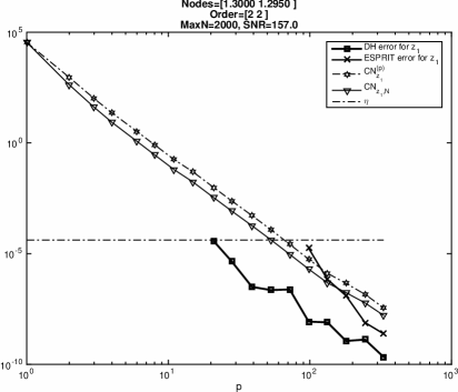
(a)

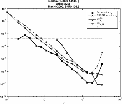
(b)

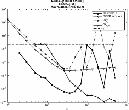
(c)

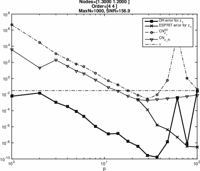
(d)

Figure 1: DH vs. ESPRIT. Also plotted are condition numbers, both full and decimated, as well as the threshold $\eta$ used in the experiments.

$p$	time (sec)	rec.error
1	1	0.005
3	8	0.001
5	25	0.0002
10	99	0.00009

(a) Exhaustive search. Pruning step only.

$p$	time (sec)	rec.error
3	0.9	0.0002
4	1.1	0.0001
6	1.1	0.0004
8	1.0	0.00008

(b) Filtering. Overall timings

Table 1: Running times for exhaustive search and filtering. The experimental setup is the same as in Figure 1b. Each table describes a separate experiment, therefore the reconstruction errors are slightly different.

$p$	ESPRIT	DH_Create	DH_Run	DH_Select
120	0.13	0.84	0.11	0.001
169	0.21	0.75	0.09	0.001
238	0.21	0.74	0.10	0.002
335	0.34	0.89	0.10	0.003

Table 2: DH vs ESPRIT timings (sec). The columns for DH correspond to the system construction, PHC run and the pruning steps.

Some additional remarks:

1. The number of solutions of the system (18) was equal to $s!d^{s}$ ($s$=number of nodes, $d=d_{j}$=degree).

2. Running times are better for DH when $p$ is large, because the selection step of Algorithm 2 is $O\left(N\right)$, while the cost of full SVD for ESPRIT is $O\left(N^{2}R\right)$. See in particular Table 2. We did not observe any unusual memory consumption during the execution of the algorithms.

3. Condition number estimates are somewhat pessimistic, nevertheless indicating the order of error decay in a relatively accurate fashion. The periodic pattern is well-predicted by the theory, see [6].

6 Discussion

In this paper we presented a novel algorithm, Decimated Homotopy, for numerical solution of systems of Prony type (1) with nodes on the unit circle, $\left|z_{j}\right|=1$ which are closely spaced. Analysis shows that the produced solutions have near-optimal numerical accuracy. Numerical experiments demonstrate that the pruning heuristics are efficient in practice, and the algorithm provides reconstruction accuracy several orders of magnitude better than the standard ESPRIT algorithm. The pruning(20) will be justified in the case that the system ${\cal H}_{p^{*}}$ has no spurious solutions on the torus $\mathbb{T}^{s}$. This seems to hold in practice, and therefore a theoretical analysis of this question would be desirable. On the other hand, initial approximations of order $\eta\approx N^{-1}$ can presumably be obtained by existing methods with lower-order multiplicity (similar to what was done in [7]).

Another important question of interest is robust detection of these near-singular situations, i.e. correct identification of the collision pattern $D$. While the integer $d$ can be estimated via numerical rank computation of the Hankel matrix $H_{d}$ (4) (see e.g. [12] and also a randomized approach [23]), the determination of the individual components of $D$ is a more delicate task, which requires an accurate estimation of the distance from the data point to the nearest “pejorative” manifold of larger multiplicity, and comparing it with the a-priori bound $\varepsilon$ on the error. We hope that the present (and future) symbolic-numeric techniques such as [15, 30], combined with description of singularities of the Prony mapping ${\cal P_{N}}$ [9], will eventually provide a satisfactory answer to this question.

As we discuss in [6], decimation is related to other similar ideas in numerical analysis [33] and signal processing [24, 25, 27]. In symbolic-numeric literature connected with sparse numerical polynomial interpolation (i.e. in the noisy setting), the possible ill-conditioning of the Hankel matrices $H_{d}$ can be overcome either by random sampling of the nodes $\left\{z_{j}\right\}$ [19, 21, 23] or by the recently introduced affine sub-sequence approach [22] for outlier detection (see also [14]), which is in many ways similar to decimation.

It would be interesting to establish more precise connections of our method to these works.

References

References

• Akinshin et al. [2015] Akinshin, A., Batenkov, D., Yomdin, Y., May 2015. Accuracy of spike-train Fourier reconstruction for colliding nodes. In: 2015 International Conference on Sampling Theory and Applications (SampTA). pp. 617–621.
• Badeau et al. [2006] Badeau, R., David, B., Richard, G., 2006. High-resolution spectral analysis of mixtures of complex exponentials modulated by polynomials. IEEE Transactions on Signal Processing 54 (4), 1341–1350.
• Badeau et al. [2008] Badeau, R., David, B., Richard, G., 2008. Performance of ESPRIT for estimating mixtures of complex exponentials modulated by polynomials. IEEE Transactions on Signal Processing 56 (2), 492–504.
• Batenkov [2014] Batenkov, D., 2014. Prony Systems via Decimation and Homotopy Continuation. In: Proceedings of the 2014 Symposium on Symbolic-Numeric Computation. SNC ’14. ACM, New York, NY, USA, pp. 59–60.
URL http://doi.acm.org/10.1145/2631948.2631961
• Batenkov [2015] Batenkov, D., 2015. Complete Algebraic Reconstruction of Piecewise-Smooth Functions from Fourier Data. Mathematics of Computation 84 (295), 2329–2350.
URL http://www.ams.org/mcom/0000-000-00/S0025-5718-2015-02948-2/
• Batenkov [2016] Batenkov, D., 2016. Stability and super-resolution of generalized spike recovery. Applied and Computational Harmonic Analysis, in press.
URL http://www.sciencedirect.com/science/article/pii/S1063520316300641
• Batenkov and Yomdin [2012] Batenkov, D., Yomdin, Y., 2012. Algebraic Fourier reconstruction of piecewise smooth functions. Mathematics of Computation 81, 277–318.
URL http://dx.doi.org/10.1090/S0025-5718-2011-02539-1
• Batenkov and Yomdin [2013] Batenkov, D., Yomdin, Y., 2013. On the accuracy of solving confluent Prony systems. SIAM J. Appl. Math. 73 (1), 134–154.
• Batenkov and Yomdin [2014] Batenkov, D., Yomdin, Y., 2014. Geometry and Singularities of the Prony mapping. Journal of Singularities 10, 1–25.
URL http://www.journalofsing.org/volume10/article1.html
• Beckermann et al. [2007] Beckermann, B., Golub, G. H., Labahn, G., Mar. 2007. On the numerical condition of a generalized Hankel eigenvalue problem. Numerische Mathematik 106 (1), 41–68.
URL http://link.springer.com/article/10.1007/s00211-006-0054-x
• Ben-Or and Tiwari [1988] Ben-Or, M., Tiwari, P., 1988. A deterministic algorithm for sparse multivariate polynomial interpolation. In: Proceedings of the twentieth annual ACM symposium on Theory of computing. ACM, pp. 301–309.
URL http://dl.acm.org/citation.cfm?id=62241
• Cadzow [1994] Cadzow, J. A., Jan. 1994. Total Least Squares, Matrix Enhancement, and Signal Processing. Digital Signal Processing 4 (1), 21–39.
URL http://www.sciencedirect.com/science/article/pii/S1051200484710037
• Candes and Fernandez-Granda [2014] Candes, E., Fernandez-Granda, C., Jun. 2014. Towards a mathematical theory of super-resolution. Communications on Pure and Applied Mathematics 67 (6), 906–956.
URL http://onlinelibrary.wiley.com/doi/10.1002/cpa.21455/abstract
• Comer et al. [2012] Comer, M. T., Kaltofen, E. L., Pernet, C., 2012. Sparse polynomial interpolation and Berlekamp/Massey algorithms that correct outlier errors in input values. In: Proceedings of the 37th International Symposium on Symbolic and Algebraic Computation. ACM, pp. 138–145.
URL http://dl.acm.org/citation.cfm?id=2442852
• Dayton et al. [2011] Dayton, B., Li, T.-Y., Zeng, Z., 2011. Multiple zeros of nonlinear systems. Mathematics of Computation 80 (276), 2143–2168.
URL http://www.ams.org/mcom/2011-80-276/S0025-5718-2011-02462-2/
• Eckhoff [1995] Eckhoff, K., 1995. Accurate reconstructions of functions of finite regularity from truncated Fourier series expansions. Mathematics of Computation 64 (210), 671–690.
• Elaydi [2005] Elaydi, S., 2005. An Introduction to Difference Equations. Springer.
• Gautschi [1962] Gautschi, W., 1962. On inverses of Vandermonde and confluent Vandermonde matrices. Numerische Mathematik 4 (1), 117–123.
• Giesbrecht et al. [2009] Giesbrecht, M., Labahn, G., Lee, W.-s., Aug. 2009. Symbolic-numeric sparse interpolation of multivariate polynomials. Journal of Symbolic Computation 44 (8), 943–959.
URL http://www.sciencedirect.com/science/article/pii/S0747717108001879
• Guan and Verschelde [2008] Guan, Y., Verschelde, J., 2008. PHClab: a MATLAB/Octave interface to PHCpack. In: Software for Algebraic Geometry. Springer, pp. 15–32.
URL http://link.springer.com/chapter/10.1007/978-0-387-78133-4_2
• Kaltofen and Lee [2003] Kaltofen, E., Lee, W.-s., Sep. 2003. Early termination in sparse interpolation algorithms. Journal of Symbolic Computation 36 (3–4), 365–400.
URL http://www.sciencedirect.com/science/article/pii/S0747717103000889
• Kaltofen and Pernet [2014] Kaltofen, E., Pernet, C., 2014. Sparse Polynomial Interpolation Codes and their decoding beyond half the minimal distance. In: ISSAC 2014 Proc. 39th Internat. Symp. Symbolic Algebraic Comput. pp. 280–287.
• Kaltofen et al. [2012] Kaltofen, E. L., Lee, W.-s., Yang, Z., 2012. Fast estimates of Hankel matrix condition numbers and numeric sparse interpolation. In: Proceedings of the 2011 International Workshop on Symbolic-Numeric Computation. ACM, pp. 130–136.
URL http://dl.acm.org/citation.cfm?id=2331704
• Kia et al. [2007] Kia, S., Henao, H., Capolino, G.-A., Aug. 2007. A high-resolution frequency estimation method for three-phase induction machine fault detection. IEEE Transactions on Industrial Electronics 54 (4), 2305–2314.
• Kim et al. [2013] Kim, Y.-H., Youn, Y.-W., Hwang, D.-H., Sun, J.-H., Kang, D.-S., Sep. 2013. High-resolution parameter estimation method to identify broken rotor bar faults in induction motors. IEEE Transactions on Industrial Electronics 60 (9), 4103–4117.
• Lee [2007] Lee, W.-s., 2007. From Quotient-difference to Generalized Eigenvalues and Sparse Polynomial Interpolation. In: Proceedings of the 2007 International Workshop on Symbolic-numeric Computation. SNC ’07. ACM, New York, NY, USA, pp. 11–116.
URL http://doi.acm.org/10.1145/1277500.1277518
• Maravic and Vetterli [2005] Maravic, I., Vetterli, M., 2005. Sampling and reconstruction of signals with finite rate of innovation in the presence of noise. IEEE Transactions on Signal Processing 53 (8 Part 1), 2788–2805.
• O’Leary and Rust [2013] O’Leary, D. P., Rust, B. W., 2013. Variable projection for nonlinear least squares problems. Computational Optimization and Applications 54 (3), 579–593.
URL http://link.springer.com/article/10.1007/s10589-012-9492-9
• Pereyra and Scherer [2010] Pereyra, V., Scherer, G., Jan. 2010. Exponential Data Fitting and Its Applications. Bentham Science Publishers.
• Pope and Szanto [2009] Pope, S. R., Szanto, A., 2009. Nearest multivariate system with given root multiplicities. Journal of Symbolic Computation 44 (6), 606–625.
URL http://www.sciencedirect.com/science/article/pii/S0747717108001491
• Potts and Tasche [2010] Potts, D., Tasche, M., 2010. Parameter estimation for exponential sums by approximate Prony method. Signal Processing 90 (5), 1631–1642.
• Prony [1795] Prony, R., 1795. Essai experimental et analytique. J. Ec. Polytech.(Paris) 2, 24–76.
• Sidi [2003] Sidi, A., 2003. Practical extrapolation methods: Theory and applications. Cambridge University Press.
• Stetter [2004] Stetter, H. J., 2004. Numerical polynomial algebra. Siam.
URL http://www.google.com/books?hl=en&lr=&id=bnBrsj_cA2gC&oi=fnd&pg=PR2&dq=stetter+numerical+polynomial+algebra&ots=QHVMS_N6TA&sig=0o-YZNlg4JPRU-W7Jsub5sBFmTs
• Stoica and Moses [2005] Stoica, P., Moses, R., 2005. Spectral analysis of signals. Pearson/Prentice Hall.
• Verschelde [2011] Verschelde, J., 2011. Polynomial homotopy continuation with PHCpack. ACM Communications in Computer Algebra 44 (3/4), 217–220.
URL http://dl.acm.org/citation.cfm?id=1940524