Chapter 0 Comb models for transport along spiny dendrites

V. MéndezUniversitat Autònoma de Barcelona. Spain A. IominTechnion - Israel Institute of Technology, Israel

1 Introduction

A comb is a simplified model for various types of natural phenomena which belong to the loopless graphs category. The comb consists of a backbone along the horizontal axis and fingers or teeth along the perpendicular direction (see Figure 1 for a two sided comb).

Figure 1: Two sided comb

Comb like models have been applied to mimic ramified structures as spiny dendrites of neuron cells [MeIo13, IoMe13] or percolation clusters with dangling bonds [WeHa86]. We are interested in the first example, where a comb structure with one sided teeth of infinite length can be used to describe the movement and binding dynamics of particles inside the spines of dendrites. These spines are small protrusions from many types of neurons located on the surface of a neuronal dendrite. They receive most of the excitatory inputs and their physiological role is still unclear although most spines are thought to be key elements in neuronal information processing and plasticity [Yu10]. Spines are composed of a head ($\sim 1$ $\mu$m) and a thin neck ($\sim 0.1$ $\mu$m) attached to the surface of dendrite (see Fig. 2).

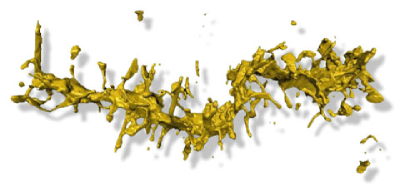
Figure 2: Electron tomogram of a spiny dendrite. Image taken from Internet (http://www.cacr.caltech.edu/projects/ldviz/results/levelsets/).

The heads of spines have an active membrane, and as a consequence, they can sustain the propagation of an action potential with a rate that depends on the spatial density of spines [EaBr09]. Decreased spine density can result in cognitive disorders, such as autism, mental retardation and fragile X syndrome [nim]. Diffusion over branched smooth dendritic trees is basically determined by classical diffusion and the mean square displacement (MSD) along the dendritic axis grows linearly with time. However, inert particles diffusing along dendrites enter spines and remain there, trapped inside the spine head and then escape through a narrow neck to continue their diffusion along the dendritic axis. Recent experiments together with numerical simulations have shown that the transport of inert particles along spiny dendrites of Purkinje and Pyramidal cells is anomalous with an anomalous exponent that depends on the density of spines [SaWi06, SaWi11, ZeHo11]. Based on these results, a fractional Nernst-Planck equation and fractional cable equation have been proposed for electrodiffusion of ions in spiny dendrites [HeLaWe08]. Whereas many studies have been focused to the coupling between spines and dendrites, they are either phenomenological cable theories [HeLaWe08, phen] or microscopic models for a single spine and parent dendrite [mic, mic2]. More recently a mesoscopic non-Markovian model for spines-dendrite interaction and an extension including reactions in spines and variable residence time have been developed [prl, MeFeHo10]. These models predict anomalous diffusion along the dendrite in agreement with the experiments but are not able to relate how the anomalous exponent depends on the density of spines [SaWi11, ZeHo11]. Since these experiments have been performed with inert particles (i.e., there are not reaction inside spines or dendrites) one concludes that the observed anomalous diffusion is due exclusively to the geometric structure of the spiny dendrite. Recent studies on the transport of particles inside spiny dendrites indicate the strong relation between the geometrical structure and anomalous transport exponents [SaWi11, bbz, kubota]. Therefore, elaboration such an analytic model that establishes this relation can be helpful for further understanding transport properties in spiny dendrites. The real distribution of spines along the dendrite, their size and shapes are completely random [nim], and inside spines the spine necks act as a transport barrier [mic]. For these reasons one may reasonably assume that the diffusion inside spine is anomalous. In this chapter, we describe some models, based on comb-like structure that mimic a spiny dendrite; where the backbone is the dendrite and the teeth (lateral branches) are the spines. The models predict: i) anomalous transport inside spiny dendrites, in agreement with the experimental results of Ref. [SaWi06], ii) also explain the dependence between the mean square displacement and the density of spines observed in [SaWi11] and iii) the mechanism of translocation wave of CaMKII (${\rm Ca}^{2+}$ - calmodulin-dependent protein kinase II, a key regulator of the synaptic function). The chapter is organized as follows. First we study the statistical properties of combs and explain how to reduce the effect of teeth on the movement along the backbone as a waiting time distribution between consecutive jumps. Second, we justify an employment of a comb-like structure as a paradigm for further exploration of a spiny dendrite. In particular, we show how a comb-like structure can sustain the phenomenon of the anomalous diffusion, reaction-diffusion and Lévy walks. Finally, we illustrate how the same models can be also useful to deal with the mechanism of ta translocation wave / translocation waves of CaMKII and its propagation failure. We also present a brief introduction to the fractional integro-differentiation in appendix at the end of the chapter.

2 Random walks in combs

The statistical properties of comb-like structures have been widely studied in the last century. The first passage-time and the survival probability were studied by some authors [WeHa86, Re01]. More recently the interest has been centered in the waiting time distribution equivalent to perform a random walk along the teeth [VdB89, CaMe05, Da07, MeFeHo10], the mean encounter time between two random walkers [Ag14] and the occupation time statistics [ReBa13]. In this section we illustrate two methods to compute the waiting time distribution that mimics the effect of a random walk along a teeth.

We first consider the case of a discrete 1D chain where the nearest neighbors are separated by a distance $a$. A random walk, where each walker moves only to one of its nearest neighbors with equal probability after a fixed waiting time $\tau$, is characterized by the following probability distribution functions (pdf)s for the waiting times and jump lengths, respectively,

$$\phi(t) = \delta(t-\tau),$$

$$w(x) = \frac{1}{2}\left[\delta(x-a)+\delta(x+a)\right].$$ (1)

In this way, systems with discrete time and space can be analyzed in terms of the Continuous-Time-Random -Walk (CTRW). Next, we add to every site of the backbone a secondary branch of length $l$, to produce a one sided comb-like structure (see Fig. 3). On such a structure, a walker that is at a given site of the backbone, can spend a certain amount of time in the secondary branch before jumping to one of the nearest neighbor sites on the backbone. If we are only interested in the behavior of the system in the direction of the backbone, then the secondary branches introduce a delay time for jumps between the neighboring sites on the backbone. The random walk on the comb structure can be modelled as a CTRW with (1) and a renormalized waiting pdf $\phi(t)$ that includes the effect of the delay due the motion along teeth.

Figure 3: Sketch of a comb structure with a nearest-neighbor distance $a$ and teeth of length $l$. The symbols $A$, $A^{\prime}$, $A^{\prime\prime}$… denote sites on the lattice (see text).

To determine analytically the effect of the teeth, we invoke convolution rules that were introduced in [VdB89] for the case of homogeneous lattices:

(i) Consider a walker that is initially at a certain site within a tooth. If the walker proceeds further into a tooth, i.e., moves away from the backbone, its probability to return to the initial site after a time $t$ is a convolution of factors, i.e., a product in the Laplace space.

(ii) The total probability for that walker to return to the initial site is determined by summing over all $t$ from $0$ to $\infty$.

(iii) When the walker reaches a crossing, where it can choose between different directions, the total probability is the sum of the probabilities for each possible direction.

The teeth have no other additional crossings. It is as shown in Fig. 3. For the sake of generality, we consider the case that when the walker is at a site on the backbone, it can jump to another site on the backbone with probability $\alpha$, or move onto the secondary branch with probability $1-\alpha$.

Without loss of generality, we assume that initially the walker is located on the backbone, and we apply the rules (i) – (iii) to determine $\phi(t)$. We study three specific cases.

(a) Comb structure with $l=a$. In this case there is only one site on the tooth, $A^{\prime}$. The walker can only jump in the direction of the backbone with probability $\alpha$ or move onto the branch with probability $1-\alpha$ and then return to the initial site at the next jump. The time it takes to reach one of the nearest neighbors on the backbone is $t=\tau$ with probability $\alpha$, $t=3\tau$ with probability $(1-\alpha)\times 1\times\alpha$, $t=5\tau$ with probability $(1-\alpha)^{2}\times 1^{2}\times\alpha$, and so on. We can write intuitively the general form $\phi(t)$ as

$$\phi(t)=\sum_{j=1}^{\infty}\alpha(1-\alpha)^{j-1}\delta\left[t-\left(2j-1\right)\tau\right].$$ (2)

The rules listed above for $\phi(t)$ should reproduce this behavior. For this purpose we need to work in the Laplace space. Let $\hat{\phi}(s)$ be the Laplace transform of $\phi(t)$. The rules (i) – (iii) lead to the expression

$$\hat{\phi}(s)=\alpha\hat{\phi}_{0}\sum_{j=0}^{\infty}\left[(1-\alpha)\hat{\phi}_{0}^{2}\right]^{j}=\frac{\alpha\hat{\phi}_{0}}{1-(1-\alpha)\hat{\phi}_{0}^{2}}\,,$$ (3)

where $\hat{\phi}_{0}$ is the probability distribution for a single jump, $\hat{\phi}_{0}=e^{-\tau s}$, which is the Laplace transform of (1).

Equation (3) is derived as follows. The term $(1-\alpha)\hat{\phi}_{0}^{2}$ in the sum represents, according to rule (i), the probability function for each occurrence of the walker moving onto the secondary branch. This expression must be summed up to infinity, according rule (ii), to take into account that the walker can move onto the tooth $1,2,...,\infty$ times. The factor $\alpha\hat{\phi}_{0}$ accounts for the final jump to the nearest neighbor on the backbone.

It is easy to see that the expression (3) may be written as a Taylor series,

$$\hat{\phi}(s)=\sum_{j=1}^{\infty}\alpha(1-\alpha)^{j-1}\left(\hat{\phi}_{0}\right)^{2j-1}\,,$$ (4)

which is the Laplace transform of (2). The method for determining $\hat{\phi}(s)$ is shown to be valid in this case.

(b) Comb structure with $l=2a$. The secondary branch is two-sites long, $A^{\prime}$ and $A^{\prime\prime}$. Similarly to the previous case we can write the distribution for the time probabilities as

$$\hat{\phi}(s)=\alpha\hat{\phi}_{0}\sum_{j=0}^{\infty}\left[\frac{(1-\alpha)}{2}\hat{\phi}_{0}^{2}\sum_{k=0}^{\infty}\left(\frac{1}{2}\hat{\phi}_{0}^{2}\right)^{k}\right]^{j}=\frac{\alpha\hat{\phi}_{0}(2-\hat{\phi}_{0}^{2})}{2-(2-\alpha)\hat{\phi}_{0}^{2}}\,.$$ (5)

In this equation a new sum over the index $k$ appears, because the walker can move away from the backbone twice. For each such occurrence we must apply rule (i). We also assume that jumps to the nearest neighbor occur with probability $1/2$ on the linear teeth.

(c) Comb structure with $l\rightarrow\infty$. Each time the walker moves away from the backbone, a new convolution factor appears in $\hat{\phi}(s)$. For the case $l\rightarrow\infty$, we have in principle infinitely many convolution factors in the expression for $\hat{\phi}(s)$. Fortunately, we can simplify this situation considerably. Assume that the walker is at the first site on the secondary branch, point $A^{\prime}$ in Fig. 3, and moves away from the backbone. Let $\eta_{A^{\prime}}$ be the probability distribution of returning for the first time to the point $A^{\prime}$ after a time $t$. Now suppose the same situation but for the initial point $A^{\prime\prime}$. It is easy to see that as $l\rightarrow\infty$ the limit $\eta_{A^{\prime\prime}}\rightarrow\eta_{A^{\prime}}$ has to hold, and we can again use the rules (i) – (iii) to determine $\eta_{A^{\prime}}$. Doing so, we obtain the expression

$$\eta_{A^{\prime}}=\frac{1}{2}\hat{\phi}_{0}\sum_{j=0}^{\infty}\left(\frac{1}{2}\hat{\phi}_{0}\eta_{A^{\prime\prime}}\right)^{j}\,.$$ (6)

This expression is equivalent to the form (3) with $\alpha=1/2$; on the secondary branch every jump to a nearest neighbor occurs with probability $1/2$. Introducing the condition $\eta_{A^{\prime\prime}}=\eta_{A^{\prime}}$, which is strictly correct for $l=\infty$, and solving (6), we find

$$\eta_{A^{\prime}}=\frac{1-\sqrt{1-\hat{\phi}_{0}^{2}}}{\hat{\phi}_{0}}\,.$$ (7)

With this result, the distribution $\hat{\phi}(s)$ is obtained straightforwardly from the three rules (i) – (iii),

$$\hat{\phi}(s)=\alpha\hat{\phi}_{0}\sum_{j=0}^{\infty}\left[(1-\alpha)\hat{\phi}_{0}\eta_{A^{\prime}}\right]^{j}=\frac{\alpha\hat{\phi}_{0}}{\alpha+\left(1-\alpha\right)\sqrt{1-\hat{\phi}_{0}^{2}}}\,.$$ (8)

In finding the waiting time pdf associated with the comb structures, it is assumed that we are only interested in the dynamical behavior along the backbone and the rest of the structure is considered as secondary.

The second method consists in finding the master equation for the random walk moving along the backbone. This master equation has to have incorporated the movement along the teeth. Consider first the simplest case of a one sided comb with a single node as shown in Figure 4

Figure 4: Comb with a single node along the tooth. In the picture are written the probabilities of jumping between nodes of length $a$.

Let $\alpha$ be the probability of moving along the backbone, when the walker is at a node of the backbone and $1-\alpha$ is the probability of jumping to the teeth, if the walker is at the backbone. So, if the movement along the backbone is considered isotropic, the probability of jumping to the right or to the left is $\alpha/2$. The master equation for the probability of finding a walker located at the node $i$ of the backbone at time $t$ is (see Figure 4)

$$P(i,t)=\frac{\alpha}{2}P(i+a,t-\tau)+\frac{\alpha}{2}P(i-a,t-\tau)+P(1,t-\tau)\,,$$ (9)

where we have taken into account that the walker waits a constant time $\tau$ at every node between consecutive jumps. The master equation for the node 1 of the tooth reads

$$P(1,t)=(1-\alpha)P(i,t-\tau)$$ (10)

that is coupled to (9). Since time is a discrete variable it is convenient to transform the time coordinate to new variable $z$ through the transformation

$$P(i,z)=\sum_{t=0}^{\infty}z^{t}P(i,t)\,.$$

Multiplying (9) and (10) by $z^{t}$ and summing from $t=0$ to infinity we have, respectively

$$P(i,z)=\frac{\alpha b}{2}P(i+a,z)+\frac{\alpha b}{2}P(i-a,z)+bP(1,z)\,,$$ (11)

$$P(1,z)=b(1-\alpha)P(i,z)\,,$$ (12)

where $b=z^{\tau}$. Inserting (12) into (11) and rearranging terms we get the following master equation for the movement along the backbone

$$\frac{1}{2}P(i+a,z)+\frac{1}{2}P(i-a,z)=P(i,z)\frac{1-(1-\alpha)b^{2}}{\alpha b}\,.$$ (13)

It is convenient to stress that (13) is actually the master equation for a walker moving on a comblike constructed by repeating the element depicted in Figure 4. Finally, we can write Eq. (13) in the Laplace space for time by taking into account that $z=e^{-s}$, so that $b=e^{-s\tau}.$ Hence, (13) becomes

$$\frac{1}{2}\hat{P}(i+a,s)+\frac{1}{2}\hat{P}(i-a,s)=\hat{P}(i,s)\frac{1-(1-\alpha)e^{-2s\tau}}{\alpha e^{-s\tau}}\,.$$ (14)

The example consists in generalizing the above structure to a tooth with $R$ nodes or length $l=aR$. Then, we consider a one sided comb with whose basic element is given in Figure 5. The master equation for the probability of finding a walker at the node $i$ of the backbone at time $t$ is, at the $z$ space

Figure 5: Comb with $R$ nodes along the teeth. In the picture are written the probabilities of jumping between nodes of length $a$.

$$P(i,z)=\frac{\alpha b}{2}P(i+a,z)+\frac{\alpha b}{2}P(i-a,z)+\frac{b}{2}P(1,z)\,.$$ (15)

At the node $R$ the master equation is

$$P(R,z)=\frac{b}{2}P(R-1,z)\,,$$ (16)

and at the nodes $R-1$ and 1 they are

$$P(R-1,z)=\frac{b}{2}P(R-2,z)+bP(R,z)\,,$$ (17)

$$P(1,z)=b(1-\alpha)P(i,z)+\frac{b}{2}P(2,z)\,.$$ (18)

At a generic node $j$ of the tooth we get

$$P(j,z)=\frac{b}{2}P(j-1,z)+\frac{b}{2}P(j+1,z)\,,$$ (19)

where $j=2,\ldots,R-2$. We may solve (19) by proposing the solution $P(j,z)=A\lambda^{j}.$ Inserting this solution we obtain the characteristic equation $\lambda^{2}-2\lambda/b+1=0$. Hence,

$$P(j,z)=A_{1}\lambda_{+}^{j}+A_{2}\lambda_{-}^{j}\,,$$ (20)

where $A_{1,2}$ are constant to be determined and

$$\lambda_{\pm}=\frac{1}{b}\left(1\pm\sqrt{1-b^{2}}\right)\,.$$

On setting $j=1$ and $j=2$ into Eq. (20), we get the system of algebraic equations for the constants $A_{1,2}$

$$A_{1}\lambda_{+}+A_{2}\lambda_{-}=P(1,z)\,,$$

$$A_{1}\lambda_{+}^{2}+A_{2}\lambda_{-}^{2}=P(2,z)\,.$$ (21)

On the other hand, by inserting (20) into (16) and (17) we get the equation relating $A_{1}$ and $A_{2}$

$$A_{1}\left[\lambda_{+}^{R-2}\left(1-\frac{3b^{2}}{4}\right)-\frac{b}{2}\left(1-\frac{b^{2}}{2}\right)\lambda_{+}^{R-3}\right]+A_{2}\left[\lambda_{-}^{R-2}\left(1-\frac{3b^{2}}{4}\right)-\frac{b}{2}\left(1-\frac{b^{2}}{2}\right)\lambda_{-}^{R-3}\right]=0\,.$$ (22)

By combining (22) and (21) we can express $P(2,z)$ in terms of $P(1,z)$ in the form $P(2,z)=h(b)P(1,z)$, where

$$h(b)=\frac{1}{b}\left[2-\frac{b^{2}(\lambda_{+}^{R}+\lambda_{-}^{R})}{\lambda_{+}^{R}+\lambda_{-}^{R}+(\lambda_{-}^{R}-\lambda_{+}^{R})\sqrt{1-b^{2}}}\right]\,.$$ (23)

Now, we are in position to get the master equation for the motion along the backbone by substituting $P(2,z)=h(b)P(1,z)$ into (18) and the result into (15). The final result is

$$\frac{1}{2}P(i+a,z)+\frac{1}{2}P(i-a,z)=\frac{1}{\alpha b}\left[1-\frac{b^{2}(1-\alpha)}{2-bh(b)}\right]P(i,z)\,.$$ (24)

We show now how to reduce the effect of the teeth on a waiting time distribution for the motion of a walker along the backbone. To this end we make use of the CTRW, and in particular, of the generalized master equation for finding a walker at point $x$ at time $t$ when it moves a 1D space

$$\frac{\partial P}{\partial t}=\int_{0}^{t}K(t-t^{\prime})\left[\int P(x-x^{\prime},t-t^{\prime})w(x^{\prime})dx^{\prime}-P(x,t^{\prime})\right]dt^{\prime}\,.$$ (25)

Considering the jump lengths distribution given in (1), for jumps between the consecutive nodes of a 1D lattice with spacing $a$ and transforming into the Laplace space in time, Eq. (25) becomes

$$\frac{1}{2}\hat{P}(i+a,s)+\frac{1}{2}\hat{P}(i-a,s)=\hat{P}(i,s)\left[\frac{s+\hat{K}(s)}{\hat{K}(s)}\right]\,,$$ (26)

where the memory kernel $K(t)$ is related to the waiting time distribution $\phi(t)$ through their Laplace transforms

$$\hat{K}(s)=\frac{s\hat{\phi}(s)}{1-\hat{\phi}(s)}\,.$$ (27)

Therefore, Eq. (26) reduces to

$$\frac{1}{2}\hat{P}(i+a,s)+\frac{1}{2}\hat{P}(i-a,s)=\hat{P}(i,s)\frac{1}{\hat{\phi}(s)}\,.$$ (28)

The waiting time distribution is obtained by comparing Eqs. (28) and (24), to get

$$\hat{\phi}(s)=\frac{\alpha b}{1-(1-\alpha)\left[1+\frac{\lambda_{-}^{R}-\lambda_{+}^{R}}{\lambda_{-}^{R}+\lambda_{+}^{R}}\sqrt{1-b^{2}}\right]}\,,$$ (29)

where $b=e^{-s\tau}$. If the one sided comb has a teeth with one node, $R=1$, thus from Eq. (29), the waiting time distribution is

$$\hat{\phi}(s)=\frac{\alpha b}{1-(1-\alpha)b^{2}}\,,$$

which coincides with the result obtained in Eq. (3). When $R=2$, then

$$\hat{\phi}(s)=\frac{\alpha b(2-b^{2})}{2-(2-\alpha)b^{2}}\,,$$

which is the same result obtained in (5). Finally, let us consider the infinite length of the teeth $R\rightarrow\infty$, or $l\gg a$. In this case, Eq. (29) reduces to

$$\hat{\phi}(s)=\frac{\alpha b}{\alpha+(1-\alpha)\sqrt{1-b^{2}}}\,,$$ (30)

that is equal to (8). In the limit of large times, $s\rightarrow 0$, the waiting time distribution in Eq. (30) reads $\hat{\phi}(s)\simeq 1-(1-\alpha)\sqrt{2s\tau}/\alpha$, which predicts anomalous diffusion along the backbone. So that, the teeth have to have an infinite length to predict anomalous diffusion along the whole comb at the asymptotically large times.

3 Comb-like models mimic spiny dendrites

As shown in previous studies, the geometric nature of spiny dendrites plays essential role in kinetics [SaWi06, SaWi11, ZeHo11, bkh, bbz, kubota]. The real distribution of spines along the dendrite, their size and shapes are completely random [nim], and inside spines, not only the spine necks but the spine itself acts as a transport barrier [SaWi11, kubota, mic]. Therefore a reasonable assumption is a consideration of anomalous diffusion along both the spines and dendrite. So, we propose models based on a comb-like structure that mimics a spiny dendrite, where the backbone is the dendrite and teeth (lateral branches) are the spines, see Fig. 6 (We distinguish between a smooth and a spiny dendrite). In this case dynamics inside teeth corresponds to spines, while the backbone describes diffusion along dendrites. Note that the comb model is an analogue of a 1D medium where fractional diffusion has been observed and explained in the framework of the CTRW [WeHa86, ArBa91, Metzler20001, luba] and making use of macroscopic descriptions [zabu] .

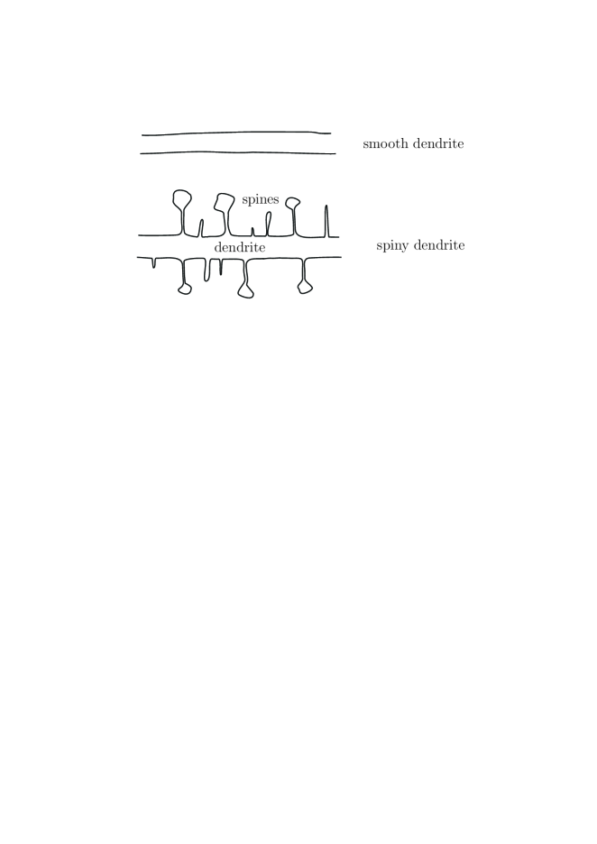
Figure 6: Draw of a smooth dendrite and a spiny dendrites

Before embarking for the CTRW consideration in the framework of the comb model, let us explain how anomalous diffusion in the comb model relates to the CaMKII transport along the spiny dendrite, and how geometry of the latter relates to the anomalous transport. As admitted above, the spine cavities behave as traps for the contaminant transport. As follows from a general consideration of a Markov process inside a finite region, the pdf of lifetimes inside the cavity with a finite volume and arbitrary form decays exponentially with time $t$ (see, for example, [Re01]) $\varphi(t)=\frac{1}{\tau}\exp(-\frac{t}{\tau}$). Here $\tau$ is a survival time (mean life time), defined by the minimum eigenvalue of the Laplace operator and determined by geometry of the cavity. For example, in Refs. [bbz, kubota], for spines with a head of volume $V$ and the cylindrical spine neck of the length $L$ and radius $a$, the mean life time is $\tau=LV/\pi a^{2}D=L^{2}/D$, where $D$ is diffusivity of the spine. Therefore, the mean probability to find a particle inside the spine after time $t$, (i.e, the survival probability inside the cavity from 0 to $t$) averaged over all possible realizations of $\tau$ is given by the integral

$$\Psi(t)=\int_{t}^{\infty}\int_{0}^{\infty}\varphi(t^{\prime}/\tau)f(\tau)d\tau dt^{\prime}$$ (31)

where $f(\tau)$ is a distribution function of the survival times $\tau$ (recall that size and shape of spines are random [nim]). Finally, the waiting time pdf can be easily calculated from Eq. (31), as follows

$$\phi(t)=-\partial_{t}\Psi(t)=\int_{0}^{\infty}\varphi(t/\tau)f(\tau)d\tau.$$ (32)

In the simplest case, when the distribution is the exponential $f(\tau)=(1/\tau_{0})\exp(-\tau/\tau_{0}$), one obtains from Eq. (32) that the general kinetics is not Markovian and the waiting time pdf is a stretched exponential for large times

$$\phi(t)=\frac{1}{\tau_{0}}\int_{0}^{\infty}\frac{e^{-t/\tau}}{\tau}e^{-\tau/\tau_{0}}d\tau=\frac{2}{\tau_{0}}K_{0}\left(2\sqrt{t/\tau_{0}}\right)\sim\left(\frac{t}{\tau_{0}}\right)^{-\frac{1}{4}}\exp(-\sqrt{t/\tau_{0}})\hskip 2.5pt,t/\tau_{0}\gg 1\hskip 2.5pt.$$

The situation is more interesting, when the distribution of the survival times is the power law $f(\tau)\sim 1/\tau^{1+\alpha},~{}(0<\alpha<1)$. In this case the waiting time pdf is the power law as well $\phi(t)\sim 1/t^{1+\alpha}$ that leads to subdiffusion motion along the dendrite. This result follows from the CTRW theory, since all underlying micro-processes are independent Markovian ones with the same distributions [Metzler20001].

Now we explain the physical reason of the possible power law distribution $\phi(t)$. At this point we paraphrase some arguments from Ref. [bAHa05] with the corresponding adaptation to the present analysis. Let us consider the escape from a spine cavity from a potential point of view, where geometrical parameters of the cavity can be related to a potential $U$. For example, for the simplest case, mentioned above, it is $U=VL/\pi a^{2}$, which “keeps” a particle inside the cavity, while $D\tau_{0}$ plays a role of the kinetic energy, or the “Boltzmann temperature”. Therefore, escape probability from the spine cavity/well is described by the Boltzmann factor $\exp(-U/D\tau_{0})$. This value is proportional to the inverse waiting, or survival time

$$t\sim\exp\left(\frac{U}{D\tau_{0}}\right).$$ (33)

As admitted above, potential $U$ is random and distributed by the Poisson distribution $P(U)=U_{0}^{-1}\exp(-U/U_{0})$, where $U_{0}$ is an averaged geometrical spine characteristic. The probability to find the waiting time in the interval $(t,t+dt)$ is equal to the probability to find the trapping potential in the interval $(U,U+dU)$, namely $\phi(t)dt=P(U)dU$. Therefore, from Eq. (33) one obtains

$$\phi(t)\sim\frac{1}{t^{1+\gamma}}\hskip 2.5pt.$$ (34)

Here $\gamma=\frac{D\tau_{0}}{U_{0}}\in(0,1)$ establishes a relation between geometry of the dendrite spines and subdiffusion observed in [SaWi06, SaWi11] and support application of the comb model, which is a convenient implement for analytical exploration of anomalous transport in spiny dendrites in the framework of the CTRW consideration.

1 Anomalous diffusion in spines

Geometry of the comb structure makes it possible to describe anomalous diffusion in spiny dendrites structure in the framework of the comb model.

Usually, anomalous diffusion on the comb is described by the $2D$ distribution function $P=P(x,y,t)$, and a special behavior is that the displacement in the $x$–direction is possible only along the structure backbone ($x$-axis at $y=0$). Therefore, diffusion in the $x$-direction is highly inhomogeneous. Namely, the diffusion coefficient is $D_{xx}=D_{x}\delta(y)$, while the diffusion coefficient in the $y$–direction (along teeth) is a constant $D_{yy}=D_{y}$. Due to this geometrical construction, the flux of particles along the dendrite is

$$J_{x}=-D_{x}\delta(y)\frac{\partial P}{\partial x}$$ (35)

and the flux along the finger describes the anomalous trapping process that occurs inside the spine

$$J_{y}=\left.-D_{y}\frac{\partial^{1-\gamma}}{\partial t^{1-\gamma}}\right|_{RL}\frac{\partial P}{\partial y}$$ (36)

where $P(x,y,t)$ is the density of particles and

$$\left.\frac{\partial^{1-\gamma}}{\partial t^{1-\gamma}}\right|_{RL}f(t)=\frac{\partial}{\partial t}I_{t}^{\gamma}f(t)$$ (37)

is the Riemann-Liouville fractional derivative, where the fractional integration $I_{t}^{\gamma}$ is defined by means of the Laplace transform

$$\hat{\mathcal{L}}\left[I_{t}^{\gamma}f(t)\right]=s^{-\gamma}\hat{f}(s)\,.$$ (38)

So, inside the spine, the transport process is anomalous and $\left\langle y^{2}(t)\right\rangle\sim t^{\gamma}$, where $\gamma\in(0,1)$. Making use of the continuity equation for the total number of particles

$$\frac{\partial P}{\partial t}+\mbox{div}\mathbf{J}=0\,,$$ (39)

where $\mathbf{J}=(J_{x},J_{y})$, one has the following evolution equation for transport along the spiny dendrite

$$\frac{\partial P}{\partial t}-D_{x}\delta(y)\frac{\partial^{2}P}{\partial x^{2}}-D_{y}\frac{\partial^{1-\gamma}}{\partial t^{1-\gamma}}\Big{|}_{RL}\frac{\partial^{2}P}{\partial y^{2}}=0.$$ (40)

The Riemann-Liouville fractional derivative in Eq. (40) is not convenient for the Laplace transform. To ensure feasibility of the Laplace transform, which is a strong machinery for treating fractional equations, one reformulates the problem in a form suitable for the Laplace transform application.

To shed light on this situation, let us consider a comb in the $3D$ [bAHa05]. This model is described by the distribution function $P_{1}(x,y,z,t)$ with evolution equation given by the equation

$$\frac{\partial P_{1}}{\partial t}-D_{x}\delta(y)\delta(z)\frac{\partial^{2}P_{1}}{\partial x^{2}}-D_{y}\delta(z)\frac{\partial^{2}P_{1}}{\partial y^{2}}-\frac{\partial^{2}P_{1}}{\partial z^{2}}=0\,.$$ (41)

It should be stressed that $z$ coordinate (do not confuse with the $z$ variable introduced in the previous section) is a supplementary, virtue variable, introduced to described fractional motion in spines by means of the Markovian process. Thus the true distribution is $P(x,y,t)=\int_{-\infty}^{\infty}P_{1}(x,y,z,t)dz$ with corresponding evolution equation

$$\frac{\partial P}{\partial t}-D_{x}\delta(y)\frac{\partial^{2}P_{1}(z=0)}{\partial x^{2}}-D_{y}\frac{\partial^{2}P_{1}(z=0)}{\partial y^{2}}=0\,.$$ (42)

A relation between $P(x,y,t)$ and $P_{1}(x,y,z=0,t)$ can be expressed through their Laplace transforms

$$\hat{P}_{1}(x,y,z=0,s)=\frac{\sqrt{s}}{2}\hat{P}(x,y,s)\,,$$ (43)

where $\hat{P}(x,y,s)=\hat{\mathcal{L}}[P(x,y,t)]$ and $\hat{P}_{1}(x,y,z,s)=\hat{\mathcal{L}}[P_{1}(x,y,z,t)]$.

Equation (43) establishes a relationship between the distributions $P_{1}(x,y,z=0,t)$ and $P(x,y,t)$ in the Laplace space. Both distributions are related through the expression

$$P\left(x,y,t\right)=\int_{-\infty}^{\infty}P_{1}\left(x,y,z,t\right)dz\,.$$

If we transform the above equation by Fourier-Laplace we get

$$\hat{P}\left(k_{x},k_{y},s\right)=\hat{P}_{1}\left(k_{x},k_{y},k_{z}=0,s\right)\,.$$ (44)

Then, Eq. (43) is nothing but a relation between $\hat{P}_{1}\left(k_{x},k_{y},k_{z}=0,s\right)$ and $\hat{P}_{1}\left(k_{x},k_{y},z=0,s\right)$. To find $\hat{P}_{1}\left(k_{x},k_{y},k_{z},s\right)$ we transform Eq. (41) by Fourier-Laplace and after collecting terms we find

$$\hat{P}_{1}\left(k_{x},k_{y},k_{z},s\right)=\frac{1-D_{x}k_{x}^{2}P_{1}\left(k_{x},y=0,z=0,s\right)-D_{y}k_{y}^{2}P_{1}\left(k_{x},k_{y},z=0,s\right)}{s+k_{z}^{2}}\,,$$ (45)

where the initial condition has been assumed $P_{1}\left(x,y,z,t=0\right)=\delta\left(x\right)\delta\left(y\right)\delta\left(z\right)$ for simplicity. Setting $k_{z}=0$ one gets

$$\hat{P}_{1}\left(k_{x},k_{y},k_{z}=0,s\right)=\frac{1-D_{x}k_{x}^{2}P_{1}\left(k_{x},y=0,z=0,s\right)-D_{y}k_{y}^{2}P_{1}\left(k_{x},k_{y},z=0,s\right)}{s}\,.$$ (46)

Inverting Eq. (45) by Fourier over $k_{z}$ we obtain

$$\hat{P}_{1}\left(k_{x},k_{y},z,s\right)=\frac{1-D_{x}k_{x}^{2}P_{1}\left(k_{x},y=0,z=0,s\right)-D_{y}k_{y}^{2}P_{1}\left(k_{x},k_{y},z=0,s\right)}{2\sqrt{s}}e^{-\sqrt{s}\left|z\right|}\,.$$

Then setting $z=0$, one obtains

$$\hat{P}_{1}\left(k_{x},k_{y},z=0,s\right)=\frac{1-D_{x}k_{x}^{2}P_{1}\left(k_{x},y=0,z=0,s\right)-D_{y}k_{y}^{2}P_{1}\left(k_{x},k_{y},z=0,s\right)}{2\sqrt{s}}\,.$$ (47)

Combining Eqs. (46) and (47), one has

$$\hat{P}_{1}\left(k_{x},k_{y},z=0,s\right)=\frac{\sqrt{s}}{2}\hat{P}_{1}\left(k_{x},k_{y},k_{z}=0,s\right)\,,$$

then the Fourier inversion over $k_{x}$ and $k_{y}$ yields Eq. (43). Finally, performing the Laplace transform of Eq. (42) one obtains

$$s\hat{P}(x,y,s)-D_{x}\delta(y)\frac{\partial^{2}\hat{P}_{1}(x,y,z=0,s)}{\partial x^{2}}-D_{y}\frac{\partial^{2}\hat{P}_{1}(x,y,z=0,s)}{\partial y^{2}}=P(x,y,t=0)\,,$$ (48)

and substituting relation (43), dividing by $\sqrt{s}$ and then performing the Laplace inversion, one obtains the comb model with the fractional time derivative

$$\frac{\partial^{\frac{1}{2}}P}{\partial t^{\frac{1}{2}}}-D_{x}\delta(y)\frac{\partial^{2}P}{\partial x^{2}}-D_{y}\frac{\partial^{2}P}{\partial y^{2}}=0\,,$$ (49)

where $2D_{x,y}\rightarrow D_{x,y}$ and the Caputo derivative $\frac{\partial^{\gamma}}{\partial t^{\gamma}}$ can be defined by the Laplace transform for $\gamma\in(0,1)$ [Mainardi19961461]

$$\hat{\mathcal{L}}\left[\frac{\partial^{\gamma}f}{\partial t^{\gamma}}\right]=s^{\gamma}\hat{f}(s)-s^{\gamma-1}f(t=0)\,.$$ (50)

The fractional transport takes place in both the dendrite $x$ direction and the spines $y$ coordinate. To make fractional diffusion in dendrite normal, we add the fractional integration $I_{t}^{1-\gamma}$ by means of the Laplace transform (38), as well $\hat{\mathcal{L}}\left[I_{t}^{1-\gamma}f(t)\right]=s^{\gamma-1}\hat{f}(s)$. This yields Eq. (49), after generalization $\frac{1}{2}\rightarrow\gamma\in(0,1)$,

$$\frac{\partial^{\gamma}P}{\partial t^{\gamma}}-D_{x}\delta(y)I_{t}^{1-\gamma}\frac{\partial^{2}P}{\partial x^{2}}-D_{y}\frac{\partial^{2}P}{\partial y^{2}}=0.$$ (51)

Performing the Fourier-Laplace transform in (51) we get

$$P(k_{x},k_{y},s)=\frac{P(k_{x},k_{y},t=0)-D_{x}k_{x}^{2}P(k_{x},y=0,s)}{s+D_{y}k_{y}^{2}s^{1-\gamma}}\,,$$ (52)

where the Fourier-Laplace image of the distribution function is defined by its arguments $\hat{\mathcal{L}}\hat{\mathcal{F}}_{x}\hat{\mathcal{F}}_{y}[P(x,y,t)]=P(k_{x},k_{y},s)$. If $P(x,y,t=0)=\delta(x)\delta(y)$, inversion by Fourier over $y$ gives

$$P(k_{x},y,s)=\frac{1-D_{x}k_{x}^{2}P(k_{x},y=0,s)}{s^{(2-\gamma)/2}\sqrt{D_{y}}}\exp\left(-\left|y\right|s^{\gamma/2}/\sqrt{D_{y}}\right).$$ (53)

Taking $y=0$ the above equation provides

$$P(k_{x},y=0,s)=\frac{1}{s^{(2-\gamma)/2}\sqrt{D_{y}}+D_{x}k_{x}^{2}}\,,$$ (54)

which yields after inserting into Eq. (52)

$$P(k_{x},k_{y},s)=\frac{1}{s+D_{y}k_{y}^{2}s^{1-\gamma}}\left(1-\frac{D_{x}k_{x}^{2}}{s^{(2-\gamma)/2}\sqrt{D_{y}}+D_{x}k_{x}^{2}}\right)\,.$$ (55)

We can calculate the density of particles at a given point $x$ of the dendrite at time $t$, namely $P(x,t)$, by integrating over $y$ in the Fourier space

$$P(k_{x},s)=P(k_{x},k_{y}=0,s)=\frac{s^{-\gamma/2}\sqrt{D_{y}}}{s^{(2-\gamma)/2}\sqrt{D_{y}}+D_{x}k_{x}^{2}}\,,$$ (56)

then

$$\left\langle x^{2}(s)\right\rangle=-\left.\frac{\partial^{2}}{\partial k_{x}^{2}}P(k_{x},s)\right|_{k_{x}=0}=\frac{2D_{x}}{\sqrt{D_{y}}}\frac{1}{s^{2-\frac{\gamma}{2}}}$$ (57)

so that

$$\left\langle x^{2}(t)\right\rangle=\frac{2D_{x}}{\sqrt{D_{y}}}t^{1-\frac{\gamma}{2}}\,.$$ (58)

Equation (58) predicts subdiffusion along the spiny dendrite that is in agreement with the experimental results reported in [SaWi06]. It should be noted that this result is counterintuitive. Indeed, subdiffusion in spines, or fingers should lead to the slower subdiffusion in dendrites, or backbone with the transport exponent less than in usual comb, since these two processes are strongly correlated. But this correlation is broken due to the fractional integration $I_{t}^{1-\gamma}$ in Eq. (51). On the other hand, if we invert (56) by Fourier-Laplace we obtain the fractional diffusion equation for $P(x,t)$

$$\frac{\partial^{1-\frac{\gamma}{2}}P}{\partial t^{1-\frac{\gamma}{2}}}=\frac{D_{x}}{\sqrt{D_{y}}}\frac{\partial^{2}P}{\partial x^{2}}\,,$$

which is equivalent to the generalized Master equation (25), in the diffusion limit:

$$\frac{\partial P}{\partial t}=\int_{0}^{t}K(t-t^{\prime})\frac{\partial^{2}P(x,t^{\prime})}{\partial x^{2}}dt^{\prime}\,,$$ (59)

if the Laplace transform of the memory kernel is given by $\hat{K}(s)=\frac{D_{x}}{\sqrt{D_{y}}}s^{\gamma/2}$, which corresponds to the waiting time pdf in the Laplace space given by

$$\hat{\phi}(s)=\frac{1}{1+\frac{\sqrt{D_{y}}}{D_{x}}s^{1-\frac{\gamma}{2}}}$$ (60)

that is $\phi(t)\sim t^{-2+\frac{\gamma}{2}}$ as $t\rightarrow\infty$. Let us employ the notation for a dynamical exponent $d_{w}$ used in [SaWi06, SaWi11]. If $d_{w}=4/(2-\gamma)$ then the MSD grows as $t^{2/d_{w}}$. On the other hand, it has been found in experiments that $d_{w}$ increases with the density of spines $\rho_{s}$ and the simulations prove that $d_{w}$ grows linearly with $\rho_{s}$. Indeed, the experimental data admits almost any growing dependence of $d_{w}$ with $\rho_{s}$ due to the high variance of the data (see Fig 5.D in [SaWi11]). Equation (58) also establishes a phenomenological relation between the second moment and $\rho_{s}$. When the density spines is zero then $\gamma=0$, $d_{w}=2$ and normal diffusion takes place. If the spine density $\rho_{s}$ increases, the anomalous exponent of the pdf (60) $1-\gamma/2=2/d_{w}$ must decrease (i.e., the transport is more subdiffusive due to the increase of $\rho_{s}$) so that $d_{w}$ has to increase as well. So, our model predicts qualitatively that $d_{w}$ increases with $\rho_{s}$, in agreement with the experimental results in [SaWi11].

2 Lévy walks on fractal comb

In this section we consider a fractal comb model [iomin2011] to take into account the inhomogeneity of the spines distribution. Here, we consider the comb model for a phenomenological explanation of an experimental situation, where we introduce a control parameter which establishes a relation between diffusion along dendrites and the density of spines. Suggesting a more sophisticated relation between the dynamical exponent and the spine density, we can reasonably suppose that the fractal dimension, due to the box counting of the spine necks, is not integer: it is embedded in the $1D$ space, thus the spine fractal dimension is $\nu\in(0,1)$. According the fractal geometry (roughly speaking), the most convenient parameter is the fractal dimension of the spine volume (mass) $\mu_{\rm spine}(x)\equiv\mu(x)\sim|x|^{\nu}$. Therefore, following Nigmatulin’s idea on a construction of a “memory kernel” on a Cantor set in the Fourier space $|k|^{1-\nu}$ [NIG92] (and further developing in Refs. [NIG98, Ren, bi2011]), this leads to a convolution integral between the non-local density of spines and the probability distribution function $P(x,y,t)$ that can be expressed by means of the inverse Fourier transform [iomin2011] $\hat{\mathcal{F}}_{x}^{-1}\left[|k_{x}|^{1-\nu}P(k_{x},y,t)\right]$. Therefore, the starting mathematical point of the phenomenological consideration is the fractal comb model

$$\frac{\partial^{\gamma}P}{\partial t^{\gamma}}-D_{x}\delta(y)I_{t}^{1-\gamma}\frac{\partial^{2}P}{\partial x^{2}}-D_{y}\frac{\partial^{2}}{\partial y^{2}}\hat{\mathcal{F}}_{k_{x}}^{-1}\left[|k_{x}|^{1-\nu}P(k_{x},y,t)\right]=0\,.$$ (61)

Performing the same analysis in the Fourier-Laplace space, presented in previous section, then Eq. (56) reads

$$P(k_{x},s)=P(k_{x},k_{y}=0,s)=\frac{s^{-\gamma/2}\sqrt{D_{y}}}{s^{(2-\gamma)/2}\sqrt{D_{y}}+D_{x}|k_{x}|^{\beta}}\,,$$ (62)

where $\beta=3/2+\nu/2$.

Contrary to the previous analysis expression (57) does not work any more, since superlinear motion is involved in the fractional kinetics. This leads to divergence of the second moment due to the Lévy flights. The latter are described by the distribution $\sim 1/|x|^{1+\beta}$, which is separated from the waiting time probability distribution $\phi(t)$. To overcome this deficiency, we follow the analysis of the Lévy walks suggested in [ZKB433, ZK1818]. We consider our exact result in Eq. (62) as an approximation obtained from the joint distribution of the waiting times and the Lévy walks. Therefore, a cutoff of the Lévy flights is expected at $|x|=t$. This means that a particle moves at a constant velocity inside dendrites not all times, and this laminar motion is interrupted by localization inside spines distributed in space by the power law.

Performing the inverse Laplace transform, we obtain solution in the form of the Mittag-Leffler function [batmen]

$$P(k_{x},t)=E_{1-\gamma/2}\left(-D|k|^{\beta}t^{1-\gamma/2}\right)\,,$$ (63)

where $D=\frac{D_{x}}{\sqrt{D_{y}}}$. For the asymptotic behavior $|k|\rightarrow 0$ the argument of the Mittag-Leffler function can be small. Note that in the vicinity of the cutoff $|x|=t$ this corresponds to the large $t$ ($|k|\sim\frac{1}{t}\ll 1$), thus we have [batmen]

$$E_{1-\gamma/2}\left(-D|k|^{\beta}t^{1-\gamma/2}\right)\approx\exp\left(-\frac{D|k|^{\beta}t^{1-\gamma/2}}{\Gamma(2-\gamma/2)}\right)\,.$$ (64)

Therefore, the inverse Fourier transform yields

$$P(x,t)\approx A_{\gamma,\nu}\frac{Dt^{1-\gamma/2}}{\Gamma(2-\gamma/2)|x|^{(5+\nu)/2}}\,,$$ (65)

where $A_{\gamma,\nu}$ is determined from the normalization condition (The physical plausibility of estimations (64) and (65) also follows from the plausible finite result of Eq. (65), which is the normalized distribution $P(x,t)\sim 1/|x|^{(3+\nu+\gamma)/2}$, where $|x|=t$). Now the second moment corresponds to integration with the cutoff at $x=t$ that yields

$$\left\langle x^{2}(t)\right\rangle=K_{\gamma,\nu}t^{\frac{3-\gamma-\nu}{2}}\,,$$ (66)

where $K_{\gamma,\nu}=\frac{4A_{\gamma,\nu}D_{x}}{(1-\nu)\Gamma(2-\gamma/2)\sqrt{D_{y}}}$ is a generalized diffusion coefficient. Transition to the absence of spines means first transition to normal diffusion in teeth with $\gamma=1$ and then $\nu=0$ that yields

$$\left\langle x^{2}(t)\right\rangle=K_{1,0}t\,.$$ (67)

3 Fractional reaction-diffusion along spiny dendrites

Geometrically, spiny dendrites in the $3D$ space are completely described by a comb structure in the $2D$, where the spine density on the cylinder surface is projected on the $1D$ axis (say the $x$ axis): $\rho(x,r={\rm const},\theta)\rightarrow\rho(x)$. Here $\rho(x,r=const,\theta)$ is the spine density, while $\rho(x)$ is the density of the comb teeth. In what follows, we consider $\rho(x)=g={\rm const}$, which is, probably, the most realistic case. Fractional diffusion inside the spines is described by fractional diffusion inside the teeth. Therefore, one considers a two-sided comb model as in Figure 1, and the starting mathematical point of the phenomenological consideration is the Fokker-Planck equation obtained in [MeIo13].

It reads,

$$\frac{\partial P}{\partial t}-\delta(y)\frac{\partial^{2}P}{\partial x^{2}}-g\frac{\partial^{2}P}{\partial y^{2}}=0\,.$$ (68)

This equation is obtained by the re-scaling with relevant combinations of the comb parameters $D_{x}$ and $D_{y}$, such that the dimensionless time and coordinates are $D_{x}^{3}t/D_{y}^{2}\rightarrow t$ $D_{x}/D_{y}\rightarrow x$, $D_{x}/D_{y}\rightarrow y/\sqrt{g}$, correspondingly [ib2005], and parameter $g$ can be considered as a constant density of the fingers.

As admitted above a variety of interactions inside spines leads to correlated noises in dendritic spines [Zeng]. The strong correlations of that leads to anomalous (subdiffusive) motion inside the spines. Following a phenomenological description by the CTRW, this subdiffusion is controlled by a waiting-time pdf $\phi(t)$ decaying according to the power law. Therefore, normal diffusion of the contaminant density $P(x,y,t)$, for example activated CaMKII, in spines is replaced by the anomalous transition term

$$g\frac{\partial^{2}P}{\partial y^{2}}\Rightarrow g\int_{0}^{t}K(t-t^{\prime})\frac{\partial^{2}P(t^{\prime})}{\partial y^{2}}dt^{\prime}\,,$$ (69)

where $K(t)$ is again the time memory kernel of the generalized master equation and is defined in (27). For subdiffusion, $\phi(t)=\frac{1}{1+t^{1+\gamma}}$ with $0<\gamma<1$ that yields [sokolov] $\hat{K}(s)=s^{1-\gamma}$.

One may recognize that Eq. (69) is a formal expression for the anomalous transport with very complicated form in the time domain, which in turn, is very inconvenient for the analytical treatment. Therefore, the comb model may be presented in the Laplace domain. Substituting Eq. (69) in Eq. (68), then performing the Laplace transform and taking into account Eq. (27), one obtains the comb model in the Laplace domain

$$s\hat{P}=\delta(y)\frac{\partial^{2}\hat{P}}{\partial x^{2}}-gs^{1-\alpha}\frac{\partial^{2}\hat{P}}{\partial y^{2}}+P_{0}\,.$$ (70)

Here $P_{0}=P(x,y,t=0)$ is the initial condition. As admitted, the kernel $\hat{K}(s)$ is problematic for the Laplace inversion, since it leads to the appearance of the initial condition. To overcome this obstacle, one multiplies Eq. (70) by $s^{\alpha-1}$ and then perform the Laplace inversion that yields

$$\int_{0}^{t}(t-t^{\prime})^{-\gamma}\left[\frac{\partial P(x,y,t^{\prime})}{\partial t^{\prime}}-\delta(y)\frac{\partial^{2}P(x,y,t^{\prime})}{\partial x^{2}}\right]dt^{\prime}=g\frac{\partial^{2}P(x,y,t)}{\partial y^{2}}\,.$$ (71)

Amending this equation by reaction term, one arrives at the integro-differential equation:

$$\int_{0}^{t}(t-t^{\prime})^{-\gamma}\left[\frac{\partial P(x,y,t^{\prime})}{\partial t^{\prime}}-\delta(y)\frac{\partial^{2}P(x,y,t^{\prime})}{\partial x^{2}}\right]dt^{\prime}=g\frac{\partial^{2}P(x,y,t)}{\partial y^{2}}+g\hat{C}\left[P(x,y,t)\right]\,,$$ (72)

which describes the $2D$ inhomogeneous reaction diffusion in the dispersive medium. Here $\hat{C}[P(x,y,t)]\equiv\hat{C}(P)$ is a reaction kinetic term. In particular, to model reaction kinetics inside dendrites, it can be considered either linear $\hat{C}(P)=CP$, or logistic $\hat{C}(P)=CP(x,y,t)[1-P(x,y,t)]$ [b2]. Integration with the power law kernel $t^{-\gamma}$ ensures anomalous diffusion in both the dendrite and spines.

In what follows we use convenient notations of fractional integro-differentiation given in Eq. (50) and the text below. Owing to this notation, from Eq. (72) the equation for $P(x,y,t)$ reads

$$\frac{\partial^{\gamma}P}{\partial t^{\gamma}}-\delta(y)I_{t}^{1-\gamma}\frac{\partial^{2}P}{\partial x^{2}}-g\frac{\partial^{2}P}{\partial y^{2}}=g\hat{C}(P)\,.$$ (73)

To give a first and brief insight on the problem of the front propagation, let us consider the linear reaction and $\gamma=1$. In this case, one obtains a “simple” solution [iom2012] for the travelling wave along the $x$ axis (inside dendrites). Introducing the total probability distribution function $P_{1}(x,t)=\int dyP(x,y,t)$, one obtains

$$P_{1}(x,t)=\frac{\sqrt{2g^{1/2}}}{\pi\sqrt{t^{1/2}}}\exp\left[\frac{x^{2}}{2\sqrt{gt}}-Cgt\right]\,.$$ (74)

This yields the coordinates of the front $x\sim t^{3/4}$ that spreads with the decaying velocity $v\sim t^{-1/4}$. This solution illustrates the asymptotic failure of the reaction-transport front propagation due to subdiffusion inside spiny dendrites.

4 Front propagation in combs

Recently, a mechanism of translocation wave of CaMKII has been suggested [pcb]. As shown, activated CaMKII contaminant travels along dendrites with additional translocation inside spines. Process of activation (the conversion of primed CaMKII to its active state) corresponds to the irreversible reaction that, in absence of spines, is described by the Fisher-Kolmogorov-Petrovskii-Piskunov (FKPP) equation (It relates also to the logistic kinetic term) [pcb]. Therefore, in the framework of the suggested above scheme of the dispersive subdiffusive comb (73), nonlinear reaction at subdiffusion in dendrites takes place along the $x$-axis bound, while subdiffusion in fingers describes the translocation inside spines. Therefore, reaction-transport equation (73) now reads

$$\frac{\partial^{\gamma}P}{\partial t^{\gamma}}-\delta(y)I_{t}^{1-\gamma}\left[D\frac{\partial^{2}P}{\partial x^{2}}+\hat{C}(P)\right]=g\frac{\partial^{2}}{\partial y^{2}}P\,.$$ (75)

Here $D$ describes the diffusivity inside dendrites, while $\hat{C}(P)=CP(1-P)$ is the nonlinear reaction term. Again, integrating over $y$ to obtain the kinetic equation for the total distribution $P_{1}(x,t)$, we have

$$\frac{\partial^{\gamma}P_{1}}{\partial t^{\gamma}}-I_{t}^{1-\gamma}\left[D\frac{\partial^{2}P_{0}}{\partial x^{2}}+\hat{C}(P_{0})\right]=0\,.$$ (76)

For the brevity, we denoted $P_{0}=P(x,y=0,t)$. Consider the fractional comb model (75) without reaction,

$$\frac{\partial^{\gamma}P}{\partial t^{\gamma}}-\delta(y)I_{t}^{1-\gamma}D\frac{\partial^{2}P}{\partial x^{2}}=g\frac{\partial^{2}}{\partial y^{2}}P\,.$$ (77)

and perform the Laplace transform, thus one obtains

$$s^{\gamma}\hat{P}-\delta(y)Ds^{\gamma-1}\frac{\partial^{2}\hat{P}}{\partial x^{2}}=g\frac{\partial^{2}\hat{P}}{\partial y^{2}}+s^{\gamma-1}\delta(x)\delta(y),$$ (78)

where for the initial condition we take $P(t=0)=\delta(x)\delta(y)$. Looking for the solution in form

$$\hat{P}(x,y,s)=\exp[-\sqrt{s^{\gamma}/g}|y|]f(x,s)\,.$$ (79)

one can see that $\hat{P}_{0}=\hat{P}(x,y=0,s)=f(x,s)$ and integration Eq. (79) over $y$ yields

$$\hat{P}_{0}(x,s)=\sqrt{\frac{s^{\gamma}}{4g}}\hat{P}_{1}(x,s).$$ (80)

Substituting (80) into (76) in the Laplace space, one gets

$$s\hat{P}_{1}-P_{1}(t=0)-\frac{Ds^{\frac{\gamma}{2}}}{2\sqrt{g}}\frac{\partial^{2}\hat{P}_{1}}{\partial x^{2}}-\frac{Cs^{\frac{\gamma}{2}}}{2\sqrt{g}}\hat{P}_{1}=-C\hat{\mathcal{L}}[P_{0}^{2}]\,.$$ (81)

Multiplying this equation by $e^{st}$ and using identity $e^{st}s^{\alpha}f(s)=\frac{\partial}{\partial t}e^{st}s^{\alpha-1}f(s)$, we integrate with the corresponding contour to obtain the inverse Laplace transform. This yields

$$\frac{\partial P_{1}}{\partial t}-\frac{1}{2\sqrt{g}}\frac{\partial}{\partial t}I_{t}^{1-\frac{\gamma}{2}}\left[D\frac{\partial^{2}P_{1}}{\partial x^{2}}+CP_{1}\right]=-\frac{C}{4g}\left[\frac{\partial}{\partial t}I_{t}^{1-\frac{\gamma}{2}}P_{1}\right]^{2}\,.$$ (82)

The nonlinear term is obtained by the following chain of transformations

$$C[P_{0}^{2}]=C\left[\hat{\mathcal{L}}^{-1}\hat{P}_{0}\right]^{2}=\frac{C}{4g}\left[\hat{\mathcal{L}}^{-1}s^{\frac{\gamma}{2}}\hat{P}_{1}\right]^{2}=\frac{C}{4g}\left[\frac{\partial}{\partial t}I_{t}^{1-\frac{\gamma}{2}}P_{1}\right]^{2}\,.$$ (83)

Note that a specific property of these transformations is an irreversibility with respect to the Laplace transform, since, as well known, the Laplace transform of the Riemann-Liouville fractional derivative involves the (quasi) initial value terms like $P_{1}(t=0)=\delta(x)$ [Metzler20001].

To evaluate the overall velocity of the asymptotic front, let us introduce a small parameter, say $\varepsilon$, at the derivatives with respect to the time and space [Fr]. To this end we re-scale $x\rightarrow x/\varepsilon$ and $t\rightarrow t/\varepsilon$, and $P_{1}(x,t)\rightarrow P_{1}^{\varepsilon}(x,t)=P_{1}\left(\frac{x}{\varepsilon},\frac{t}{\varepsilon}\right)$. Therefore, one looks for the asymptotic solution in a form of the Green approximation,

$$P_{1}^{\varepsilon}(x,t)=\exp\left[-\frac{G^{\varepsilon}(x,t)}{\varepsilon}\right]\,.$$ (84)

The main strategy of implication of this construction is the limit $\varepsilon\rightarrow 0$, one has $\exp\left[-\frac{G^{\varepsilon}(x,t)}{\varepsilon}\right]=0$, except the condition when $G^{\varepsilon}(x,t)=0$. This equation determines the position of the reaction spreading front, see Eq. (74). Moreover, we consider the limit $G(x,t)=\lim_{\varepsilon\to 0}G^{\varepsilon}(x,t)$ as the principal Hamiltonian function [Fr] that makes it possible to apply the Hamiltonian approach for calculation of the propagation front velocity. In this case partial derivatives of $G(x,t)$ with respect to time and coordinate have physical senses of the Hamiltonian and momentum:

$$\frac{\partial G(x,t)}{\partial t}=-H~{}~{}~{}~{}\mbox{and}~{}~{}~{}~{}\frac{\partial G(x,t)}{\partial x}=p\,.$$ (85)

Now the method of the hyperbolic scaling, explained above, can be applied. Therefore, we have the ansatz (84) for the probability distribution function inside dendrites. Inserting expression (84) in Eq. (82), one considers fractional integrations in time. Let us start from the last term in Eq. (82), which is the reaction term. We rewrite it in the following convenient form

$$\frac{\varepsilon}{\Gamma(1-\frac{\gamma}{2})}\frac{\partial}{\partial t}\int_{0}^{\frac{t}{\varepsilon}}dt^{\prime}(t^{\prime})^{-\gamma/2}\exp[-G^{\varepsilon}(t-\varepsilon t^{\prime},x-\varepsilon x^{\prime})/\varepsilon]\,.$$ (86)

Then performing expansion

$$G^{\varepsilon}(t-\varepsilon t^{\prime},x-\varepsilon x^{\prime})\approx G^{\varepsilon}(x,t)-\varepsilon\frac{\partial G^{\varepsilon}(x,t)}{\partial t}t^{\prime}-\varepsilon\frac{\partial G^{\varepsilon}(x,t)}{\partial x}x^{\prime}\,,$$

and substituting this in Eq. (86), one obtains

$$\frac{1}{\Gamma(1-\frac{\gamma}{2})}\left[-\frac{\partial G^{\varepsilon}(x,t)}{\partial t}\right]\exp\left[-\frac{G^{\varepsilon}(x,t)}{\varepsilon}\right]\int_{0}^{\frac{t}{\varepsilon}}(t^{\prime})^{-\gamma/2}\exp\left[\frac{\partial G^{\varepsilon}(x,t)}{\partial t}t^{\prime}+\frac{\partial G^{\varepsilon}(x,t)}{\partial x}x^{\prime}\right]dt^{\prime}\,.$$ (87)

It should be noted that we neglect differentiation of the upper limit of the integral, since this term is of the order of $O(\varepsilon^{1+\gamma/2})\sim o(\varepsilon)$ that vanishes in the limit $\varepsilon\rightarrow 0$. The same procedure of expansion is performed for the diffusion term in Eq. (82) that yields

$$\frac{\varepsilon^{3}}{\Gamma(1-\frac{\gamma}{2})}\frac{\partial^{3}}{\partial t\partial x^{2}}\exp\left[-\frac{G^{\varepsilon}(x,t)}{\varepsilon}\right]\int_{0}^{\frac{t}{\varepsilon}}(t^{\prime})^{-\frac{\gamma}{2}}\exp\left[\frac{\partial G^{\varepsilon}(x,t)}{\partial t}t^{\prime}+\frac{\partial G^{\varepsilon}(x,t)}{\partial x}x^{\prime}\right]dt^{\prime}\,.$$ (88)

Differentiating in the limit $\varepsilon\rightarrow 0$ and taking into account that the Hamiltonian $H$ and the momentum $p$ in Eq. (85) are independent of $x$ and $t$ explicitly (that leads to the absence of mixed derivatives), one obtains the Laplace transform of the subdiffusive kernel $t^{-\frac{\gamma}{2}}$. After these procedures in Eqs. (87) and (88), the kinetic equation (82) becomes a kind of Hamilton-Jacobi equation that establishes a relation between the Hamiltonian and the momentum

$$H=\left[\frac{Dp^{2}+C}{2\sqrt{g}}\right]^{\frac{2}{2-\gamma}}\,,$$ (89)

and the action is $G(x,t)=\int_{0}^{t}[p(s)\dot{x}(s)-H(p(s),x(s))]ds$. The rate $v$ at which the front moves is determined at the condition $G(x,t)=0$. Together with the Hamilton equations, this yields

$$v=\dot{x}=\frac{\partial H}{\partial p}\,,~{}~{}~{}v=\frac{H}{p}\,.$$ (90)

Note that the first equation in (90) reflects the dispersion condition, while the second one is a result of the asymptotically free particle dynamics, when the action is $G(x,t)=px-Ht$. Taking into account $x=vt$, one obtains Eq. (90) (see also details of this discussion e.g. in Refs. [CFM, ana]). Combination of these two equations can be replaced by

$$v=\min_{H>0}\frac{H}{p(H)}=\min_{p>0}\frac{H(p)}{p}\,.$$ (91)

We also have from the front velocity conditions (90) $\frac{\partial}{\partial p}\ln H=1/p$ that, eventually, yields from Eq. (91)

$$v=\left[\left(\frac{4}{g}\right)^{\frac{2}{2-\gamma}}\frac{D}{2-\gamma}\left(\frac{C}{2+\gamma}\right)^{\frac{2+\gamma}{2-\gamma}}\right]^{\frac{1}{2}}\,.$$ (92)

To proceed, we first, admit that the limiting case of this result with $\gamma=0$ corresponds to the CaMKII propagation along the dendrite only (i.e., there are no teeth). Therefore, Eq. (92) after rescaling $D/\sqrt{g}\rightarrow D$ and $C/\sqrt{g}\rightarrow C$ recovers the FKPP scheme for $\gamma=0$ that yields $v=\sqrt{DC}$.

It should be admitted the absence of the failure of the activation front propagation. It has a simple explanation due to the absence of a reaction “sink” term $-hP$ in Eq. (75) by neglecting the possibility of spines to accumulate a large amount of ${\rm Ca}^{2+}$ [segal1, segal2], where $h$ is a translocation/accumulation rate [pcb]. Introducing this term in Eq. (75), our anticipation is that the hyperbolic scaling for this new equation yields a solution similar to Eq. (91) with $H=0$ that corresponds to the failure of the front propagation. Moreover, this asymptotic solution for $P_{1}(x,t)$ always takes place, as one of possible solutions.

Inserting the sink term in Eq. (75), one obtains

$$\frac{\partial^{\gamma}P}{\partial t^{\gamma}}-\delta(y)I_{t}^{1-\gamma}\left[D\frac{\partial^{2}P}{\partial x^{2}}+CP(1-P)\right]-g\frac{\partial^{2}P}{\partial y^{2}}-ghP=0\,.$$ (93)

Repeating the same procedures of the Laplace transform and integration over $y$ with definition $\hat{P}_{1}=\int_{-\infty}^{\infty}\hat{P}(x,y,s)dy$, and using the substitute

$$P_{1}(x,s)=2\sqrt{g/s^{\gamma}}P(x,y=0,s)\,,$$

one obtains

$$s\hat{P}_{1}-\delta(x)=\frac{D\sqrt{s^{\gamma}}}{2\sqrt{g}}\frac{\partial\hat{P}_{1}}{\partial x^{2}}+\frac{C\sqrt{s^{\gamma}}}{2\sqrt{g}}\hat{P}_{1}-hgs^{1-\gamma}\hat{P}_{1}\,.$$ (94)

Here we neglect the nonlinear term, since, as follows from the above analysis, in the further hyperbolic scaling approximation, this term does not contribute to the Hamilton-Jacobi equation, and we also know how to handle it. Again multiplying this equation by $e^{st}$ and using the same identity $e^{st}s^{\alpha}f(s)=\frac{\partial}{\partial t}e^{st}s^{\alpha-1}f(s)$, as above, we obtain the inverse Laplace transform. Thus, Eq. (94) reads

$$\frac{\partial P_{1}}{\partial t}=\frac{D}{2\sqrt{g}}\frac{\partial}{\partial t}I_{t}^{1-\frac{\gamma}{2}}\left[\frac{\partial P_{1}}{\partial x^{2}}+\frac{C}{D}P_{1}\right]-hg\frac{\partial}{\partial t}I_{t}^{\gamma}P_{1}\,.$$ (95)

Application of the hyperbolic scaling with the asymptotic solution (84) yields

$$2\sqrt{g}H=\left[Dp^{2}H^{\frac{\gamma}{2}}+CH^{\frac{\gamma}{2}}-2hg^{\frac{3}{2}}H^{1-\gamma}\right]\,.$$ (96)

Let us consider a specific case $\gamma=2/3$ that yields

$$H=\left[\frac{Dp^{2}+C-2hg^{\frac{3}{2}}}{2\sqrt{g}}\right]^{\frac{3}{2}}.$$ (97)

For $C>2hg^{\frac{3}{2}}$ there is no failure and the front asymptotically propagates with a constant velocity. For $C\leq 2hg^{\frac{3}{2}}$ the only solution is $H=0$ and yields $v=0$. So, $2hg^{\frac{3}{2}}$ is the minimum reaction rate necessary to sustain propagation along the spiny dendrite due to the presence of translocation. Analogously, $(C/2h)^{2/3}$ can also be viewed as the minimum value for the density of spines necessary to have propagation failure. Both results are in agreement with the results obtained from very different models based on the cable model [cb].

In general case, one compares the interplay between the activation $CH^{\frac{\gamma}{2}}$ and the translocation $-2hg^{\frac{3}{2}}H^{1-\gamma}$ terms in Eq. (96) in the limit $H\rightarrow 0$. For $\gamma\in[\frac{2}{3},1)$, the translocation term is dominant and leads to the solution with $H=0$ and the failure of the front propagation, correspondingly. When $0<\gamma<\frac{2}{3}$, the activation in dendrites can be dominant. This situation is more complicated, and the activation-translocation front can propagate with an asymptotically finite velocity.

Finally, let us consider the linear counterpart of Eq. (75) with the linear reaction term $\hat{C}(P)=CP$. This analysis will be useful to uncover the behavior of the tail of the total distribution and check if the front accelerates or travel with constant velocity. Rewrite the equation for the total distribution $P_{1}(x,t)$. As follows from the fractional differentiation of Eq. (82), this equation reads (see also [MeIo13])

$$\frac{\partial^{1-\frac{\gamma}{2}}P_{1}}{\partial t^{1-\frac{\gamma}{2}}}=\frac{D}{2\sqrt{g}}\left[\frac{\partial^{2}}{\partial x^{2}}+\frac{C}{D}\right]P_{1}\,,$$ (98)

with the initial condition $P_{1}(x,t=0)=\delta(x)$. After the Fourier transform $\hat{\mathcal{F}}[P_{1}(x,t)]=\bar{P}_{1}(k,t)$, one obtains the solution in the form of the Mittag-Leffler function

$$\bar{P}_{1}(k,t)=E_{1-\frac{\gamma}{2}}\left[A(k)t^{1-\frac{\gamma}{2}}\right]\,,$$ (99)

where $A(k)=(C-Dk^{2})/2\sqrt{g}$. At the asymptotic condition, when $x\,,t\gg 1$, we have $C\gg Dk^{2}$ that yields asymptotic behavior of the Mittag-Leffler function as a growing exponent (for the large positive argument) [batmen]

$$\bar{P}_{1}(k,t)\approx\exp\left[\left(\frac{C}{2\sqrt{g}}-\frac{D}{2\sqrt{g}}k^{2}\right)^{\frac{2}{2-\gamma}}t\right]\approx\exp\left[\left(\frac{C}{2\sqrt{g}}\right)^{\frac{2}{2-\gamma}}\left(1-\frac{2}{2-\gamma}\frac{Dk^{2}}{C}\right)t\right]\,.$$ (100)

After the Fourier inversion, one obtains

$$P_{1}(x,t)=\exp\left[\left(\frac{C}{2\sqrt{g}}\right)^{\frac{2}{2-\gamma}}t-\frac{(2-\gamma)x^{2}(2\sqrt{g})^{\frac{2}{2-\gamma}}}{8DC^{\frac{\gamma}{2-\gamma}}t}\right]$$ (101)

that, finally, yields the nonzero and constant overall velocity of the reaction front propagation. Note that for normal diffusion, $\gamma=0$, one arrives at the Fisher velocity $v=\sqrt{DC/g}\rightarrow\sqrt{DC}$, see limiting case $\gamma=0$ in Eq. (92).

5 Conclusion

In this chapter we show that a comb is a convenient model for analytical exploration of anomalous transport and front propagation phenomena along spiny dendrites. We have studied the properties of a random walk motion along the backbone in presence of teeth. Teeth are lateral branches crossing the backbone and we have shown here that their effect on the movement along the whole structure can be reduced to a waiting time distribution at the nodes of the backbone during the movement of the random walker. Recent experiments and numerical simulations have predicted anomalous diffusion along spiny dendrites.

We have shown here that this anomalous phenomenon can be explained in the framework of a comb model with infinitely long teeth. Moreover, due to the random distribution of spines along the parent dendrite and the presence of binding reaction inside spines one can present a physically reasonable justification of the power law of the waiting time distribution that leads to subdiffusion in both the teeth and the backbone.

We have shown how to predict anomalous diffusion in spines by constructing a fractional-diffusion equation. By using the CTRW formalism we have computed the mean square displacement for the transport along the whole comb. We presented an illustration of how to take into account the inhomogeneous distribution of spines along the dendrite by using a fractal comb. We have also constructed the corresponding fractional-diffusion equations and computed the mean square displacement. From the other hand, the constructed toy models are simple enough, like the comb model that makes it possible to suggest and understand a variety of reaction-transport schemes, including anomalous transport, by applying a strong machinery of fractional calculus and hyperbolic scaling for asymptotic methods. This approach allows to suggest an analytical description of reaction-transport scenarios in spiny dendrites, where we consider both a linear reaction in spines, see Eqs. (72) and (73), and nonlinear reaction along dendrites, considered in the framework of the FKPP scheme [Fisher1937]. To this end we suggest a fractional subdiffusive comb model, where we apply a Hamilton-Jacobi approach to estimate the overall velocity of the reaction front propagation. We proposed an alternative approach of a recently suggested mechanism of translocation wave of CaMKII [pcb], where activated CaMKII contaminant travels along dendrites with additional translocation inside spines, and process of activation corresponds to the irreversible reaction described by the FKPP equation (82). One of the main effect, observed in the framework of the considered model, is the failure of the front propagation due to either the reaction inside spines, or interaction of reaction with spines. In the first case the spines are the source of reactions, while in the latter case the spines are a source of damping, for example they act as a sink of an activated contaminant (CaMKII). The situation is controlled by three parameters CaMKII activation $C$, CaMKII translocation rate $h$ and the fractional transport exponent $\gamma$. The latter reflects the geometrical structure of the transport system: when $0<\gamma<\frac{2}{3}$, the activation in dendrites can be dominant, and the activation-translocation front can propagate with an asymptotically nonzero and constant velocity. For $\gamma=2/3$ we have found a criteria for the emergence of propagation failure or for the sustain of the propagation in terms of the reaction rate, the translocation rate and the spine’s density.

It should be admitted, in conclusion, that physical arguments suggested above, explain why anomalous transport, namely subdiffusion, of either CaMKII or neutral particles is possible and support implementation of the comb model. These arguments are based on geometry of dendritic spines that determines an expression for the transport exponent in Eq. (34). This situation becomes more sophisticated in a case of the nonlinear FKPP reaction. Indeed, as shown, the power law kernel of the transition probability considered due to the geometry arguments is insensitive to the nonlinear reaction. This consideration differs completely from a mesoscopic non-Markovian approach, developed in [prl, MeFeHo10], where spines-dendrite interaction and an extension including reactions in spines have been described in framework of variable residence time. This leads to essential complication of the transition probability due to the nonlinear reaction term [fedotov2010a, MeFeHo10].

6 Appendix: Fractional integro–differentiation

The consideration of a non-Markovian process in the framework of kinetic equations leads to the study of the so-called fractional Fokker-Planck equation, where both time and space processes are not local [Metzler20001]. In this case, derivations are substituted by integrations with the power law kernels. One arrives at so-called fractional integro–differentiation.

A basic introduction to fractional calculus can be found, e.g., in Ref. [podlubny]. Fractional integration of the order of $\alpha$ is defined by the operator

$${}_{a}I_{t}^{\alpha}f(t)=\frac{1}{\Gamma(\alpha)}\int_{a}^{t}f(\tau)(t-\tau)^{\alpha-1}d\tau,~{}~{}(\alpha>0)\,,$$ (102)

where $\Gamma(\alpha)$ is a gamma function. There is no constraint on the limit $a$. In our consideration, $a=0$ since this is a natural limit for the time. A fractional derivative is defined as an inverse operator to ${}_{a}I_{t}^{\alpha}\equiv I_{t}^{\alpha}$ as $\frac{d^{\alpha}}{dt^{\alpha}}=I_{t}^{-\alpha}=D_{t}^{\alpha}$; correspondingly $I_{t}^{\alpha}=\frac{d^{-\alpha}}{dt^{-\alpha}}=D_{t}^{-\alpha}$. Its explicit form is convolution

$$D_{t}^{\alpha}=\frac{1}{\Gamma(-\alpha)}\int_{0}^{t}\frac{f(\tau)}{(t-\tau)^{\alpha+1}}d\tau\,.$$ (103)

For arbitrary $\alpha>0$, this integral is, in general, divergent. As a regularization of the divergent integral, the following two alternative definitions for $D_{t}^{\alpha}$ exist [Mainardi19961461]

$${}_{RL}D_{(0,t)}^{\alpha}f(t)\equiv D_{RL}^{\alpha}f(t)=D^{n}I^{n-\alpha}f(t)\frac{1}{\Gamma(n-\alpha)}\frac{d^{n}}{dt^{n}}\int_{0}^{t}\frac{f(\tau)d\tau}{(t-\tau)^{\alpha+1-n}}\,,$$ (104)

$$D_{C}^{\alpha}f(t)=I^{n-\alpha}D^{n}f(t)\frac{1}{\Gamma(n-\alpha)}\int_{0}^{t}\frac{f^{(n)d\tau}(\tau)}{(t-\tau)^{\alpha+1-n}}\,,$$ (105)

where $n-1<\alpha<n,~{}~{}n=1,2,\dots$. Eq. (104) is the Riemann–Liouville derivative, while Eq. (105) is the fractional derivative in the Caputo form [Mainardi19961461]. Performing integration by part in Eq. (104) and then applying Leibniz’s rule for the derivative of an integral and repeating this procedure $n$ times, we obtain

$$D_{RL}^{\alpha}f(t)=D_{C}^{\alpha}f(t)+\sum_{k=0}^{n-1}f^{(k)}(0^{+})\frac{t^{k-\alpha}}{\Gamma(k-\alpha+1)}\,.$$ (106)

The Laplace transform can be obtained for Eq. (105). If $\hat{\mathcal{L}}[f(t)]=\tilde{f}(s)$, then

$$\hat{\mathcal{L}}\left[D_{C}^{\alpha}f(t)\right]=s^{\alpha}\tilde{f}(s)-\sum_{k=0}^{n-1}f^{(k)}(0^{+})s^{\alpha-1-k}\,.$$ (107)

The following fractional derivatives are helpful for the present analysis

$$D_{RL}^{\alpha}[1]=\frac{t^{-\alpha}}{\Gamma(1-\alpha)}\,,~{}~{}D_{C}^{\alpha}[1]=0\,.$$ (108)

We also note that

$$D_{RL}^{\alpha}t^{\beta}=\frac{t^{\beta-\alpha}\Gamma(\beta+1)}{\Gamma(\beta+1-\alpha)}\,,$$ (109)

where $\beta>-1$ and $\alpha>0$. The fractional derivative from an exponential function can be simply calculated as well by virtue of the Mittag–Leffler function (see e.g., [podlubny, batmen]):

$$E_{\gamma,\delta}(z)=\sum_{k=0}^{\infty}\frac{z^{k}}{\Gamma(\gamma k+\delta)}\,.$$ (110)

Therefore, we have the following expression

$$D_{RL}^{\alpha}e^{\lambda t}=t^{-\alpha}E_{1,1-\alpha}(\lambda t)\,.$$ (111)