Spin models in three dimensions:
Adaptive lattice spacing

Abstract

Aiming at the study of critical phenomena in the presence of boundaries with a non-trivial shape we discuss how lattices with an adaptive lattice spacing can be implemented. Since the parameters of the Hamiltonian transform non-trivially under changes of the length-scale, adapting the lattice spacing is much more difficult than in the case of the numerical solution of partial differential equations, where this method is common practice.

Here we shall focus on the universality class of the three-dimensional Ising model. Our starting point is the improved Blume-Capel model on the simple cubic lattice. In our approach, the system is composed of sectors with lattice spacing $a$, $2a$, $4a$, … . We work out how parts of the lattice with lattice spacing $a$ and $2a$, respectively, can be coupled in a consistent way. Here, we restrict ourself to the case, where the boundary between the sectors is perpendicular to one of the lattice-axis. Based on the theory of defect planes one expects that it is sufficient to tune the coupling between these two regions. To this end we perform a finite size scaling study. However first numerical results show that slowly decaying corrections remain. It turns out that these corrections can be removed by adjusting the strength of the couplings within the boundary layers.

As benchmark, we simulate films with strongly symmetry breaking boundary conditions. We determine the magnetization profile and the thermodynamic Casimir force. For our largest thickness $L_{0}=64.5$, we find that results obtained for the homogeneous system are nicely reproduced.

I Introduction

The present work is motivated by the numerical study of effects related to critical phenomena in the presence of boundaries with non-trivial shapes. Our own interest in this problem stems from an ongoing project on the thermodynamic Casimir effect R1 ; R2 ; R3 ; R4 involving finite objects. In particular, in ref. mysphere we studied the thermodynamic Casimir force between a sphere and a plane by using Monte Carlo simulations of the improved Blume-Capel model on a simple cubic lattice.

In the numerical study of partial differential equations often adaptive grids are used. In regions, where the field varies strongly, a finer resolution of the space is used than in regions, where the field is smooth. In fact, solving problems related to the thermodynamic Casimir effect in the mean-field approximation, a finite element method with a mesh adapted to the problem is used. For recent work on three-body interactions see for example refs. MaHaDi13 ; MaHaDi14 .

In the case of critical phenomena, beyond the mean-field approximation, this approach is complicated by the fact that fields and the strength of the interaction transform in a non-trivial way under a rescaling of the length. Therefore it is hard to solve the problem in general. Here we consider the Ising universality class in three dimensions and in particular study the improved Blume-Capel model. We have chosen a rather simple setup. We start from a simple cubic lattice with the lattice spacing $a$. Certain regions of the lattice are coarse grained and the lattice spacing is increased to $2a$, $4a$, … . These regions are composed of cubes with faces parallel to the $(100)$, $(010)$, and $(001)$ planes. Here we perform a first step of this program. We study how to couple two half spaces with lattice spacing $a$ and $2a$, respectively. To this end, we employ finite size scaling to determine the proper values of the couplings at the boundary between the two different lattice spacings.

In principle the boundary between lattice spacing $a$ and $2a$ can be seen as a defect plane. As argued in refs. BuEi81 ; DiDiEi83 such a defect is a relevant perturbation of the non-trivial fixed point that characterizes the continuous phase transition of the bulk systems. Its RG-exponent is $y_{d}=y_{t}-1$, where $y_{t}=1/\nu$ and $\nu$ is the critical exponent of the correlation length of the bulk system. This suggests that it is sufficient to tune the coupling between the regions with lattice spacing $a$ and $2a$. In our finite-size scaling study we consider a lattice of the size $L_{0}\times L_{1}\times L_{2}$, where $L_{0}=2L$ and $L_{1}=L_{2}=L$. We split the lattice in two halfs in $0$-direction. In one half we use lattice spacing $a$, while in the other one the lattice spacing is $2a$. We define phenomenological couplings that are suitable to detect correlations between the two parts of the lattice with different lattice spacing. First numerical results show that there are slowly decaying corrections. It turns out that these can be eliminated by tuning the couplings within the lattice planes at the boundary.

Finally we benchmark our result by simulating films with strongly symmetry breaking boundary conditions. We replace half of the sites, located in the middle of the film, by coarse grained ones. We compute the thermodynamic Casimir force and the magnetization profile. These are compared with estimates that we obtained in ref. myRecent for the homogeneous system.

The paper is organized as follows. First we define the Blume-Capel model and summarize relevant previous work. Next we introduce the finite size scaling method used to determine the couplings at the boundary between different lattice spacings. Then we discuss our simulations and the numerical results. We summarize our estimates for the couplings at the boundary between different lattice spacings. Then we present our simulations of films with strongly symmetry breaking boundary conditions. Finally we conclude and sketch how we shall use our outcome in upcoming studies of the thermodynamic Casimir force.

II The model

We consider the Blume-Capel model on a simple cubic lattice. The reduced Hamiltonian is given by

$$H=-\beta\sum_{<xy>}s_{x}s_{y}+D\sum_{x}s_{x}^{2}-h\sum_{x}s_{x}\;\;,$$ (1)

where $s_{x}\in\{-1,0,1\}$ and $x=(x_{0},x_{1},x_{2})$ denotes a site on the simple cubic lattice, where $x_{i}$ takes integer values and $<xy>$ is a pair of nearest neighbors on the lattice. The partition function is given by $Z=\sum_{\{s\}}\exp(-H)$, where the sum runs over all spin configurations. The parameter $D$ controls the density of vacancies $s_{x}=0$. In the limit $D\rightarrow-\infty$ vacancies are completely suppressed and hence the spin-1/2 Ising model is recovered. Here we consider a vanishing external field $h=0$ throughout. In $d\geq 2$ dimensions the model undergoes a continuous phase transition for $-\infty\leq D<D_{tri}$ at a $\beta_{c}$ that depends on $D$. For $D>D_{tri}$ the model undergoes a first order phase transition, where for the three-dimensional lattice $D_{tri}=2.0313(4)$ DeBl04 .

Numerically, using Monte Carlo simulations it has been shown that there is a point $(D^{*},\beta_{c}(D^{*}))$ on the line of second order phase transitions, where the amplitude of leading corrections to scaling vanishes. Our recent estimate is $D^{*}=0.656(20)$ mycritical . In mycritical we simulated the model at $D=0.655$ close to $\beta_{c}$ on lattices of a linear size up to $L=360$. From a standard finite size scaling analysis of phenomenological couplings like the Binder cumulant we find $\beta_{c}(0.655)=0.387721735(25)$. Furthermore the amplitude of leading corrections to scaling is at least by a factor of $30$ smaller than for the spin-1/2 Ising model. In the following study we shall simulate at $D=0.655$ throughout.

III The finite size scaling method

We study lattices of the size $L_{0}=2L$ and $L_{1}=L_{2}=L$ with periodic boundary conditions in all three directions. In order to get numbers to compare with, we simulated a lattice with a unique lattice spacing $a=1$ first.

Next we studied a lattice with the lattice spacing $a=1$ for $0\leq x_{0}<L$ and lattice spacing $2a=2$ for $L\leq x_{0}<2L$. In the following we shall refer to the fine and the coarse part of the lattice simply by fine or coarse lattice, respectively. The sites of the fine lattice are located at $x_{0}=0.5,1.5,...,L-0.5$, while those of the coarse lattice assume the positions $X_{0}=L+1,L+3,...,2L-1$. Between the two parts of the lattice there are two boundaries that are perpendicular to the $0$-axis and are located at $x_{0}=0$ and $x_{0}=L$.

The coupling constant in the bulk of the fine lattice is called $\beta_{1}$, the coupling constant in the bulk of the coarse lattice is called $\beta_{2}$. The coupling between the fine and the coarse lattice is denoted by $\beta_{1,2}$. It turned out that also the couplings within the layers next to the boundaries have to be tuned. They are denoted by $\beta_{1,b}$ and $\beta_{2,b}$, respectively. We parameterize these couplings by $\beta_{i,b}=c_{i,b}\beta_{i}$. This means that the reduced Hamiltonian of our system is given by

$$H = -\beta_{1}\sum_{<xy>\in I_{1}}s_{x}s_{y}-\beta_{2}\sum_{<XY>\in I_{2}}S_{X}S_{Y}-\beta_{1,b}\sum_{<xy>\in B_{1}}s_{x}s_{y}-\beta_{2,b}\sum_{<XY>\in B_{2}}S_{X}S_{Y}$$ (2)

$$-\beta_{1,2}\sum_{<xY>}s_{x}S_{Y}+D\sum_{x}s_{x}^{2}+D\sum_{X}S_{X}^{2}$$

where $I_{1}$ and $I_{2}$ denote the set of links in the interior of the fine and the coarse lattice, respectively. $B_{1}$ and $B_{2}$ denote the set of links within the layers next to the boundaries. The subscripts $1$ and $2$ indicate the fine and the coarse lattice, respectively. Sites of the fine lattice are denoted by $x$ and $y$, while those of the coarse one are denoted by $X$ and $Y$. A site in the coarse lattice, adjacent to the boundary, is coupled to four sites of the fine one. The spins on the coarse lattice are $S_{X}\in\{-1,0,1\}$. In Fig. 1 we give a two-dimensional sketch.

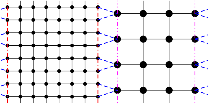
Figure 1: We give a two-dimensional sketch of the lattice with two lattice spacings. The couplings in the bulk of the fine and the coarse lattice are denoted by $\beta_{1}$ and $\beta_{2}$, respectively. The couplings within the layers at the boundary between the two parts of the lattice are denoted by $\beta_{1,b}$ and $\beta_{2,b}$, respectively. The corresponding links are given by dash-dotted lines in the sketch. The coupling between the fine and the coarse lattice are denoted by $\beta_{1,2}$. The corresponding links are indicated by blue dashed lines.

Next we define the quantities that we computed. We consider the magnetization in the center of the fine lattice

$$M_{1}=\sum_{L/4<x_{0}<3L/4,x_{1},x_{2}}s_{x}$$ (3)

and the magnetization in the center of the coarse lattice

$$M_{2}=\sum_{L+L/4<X_{0}<L+3L/4,X_{1},X_{2}}s_{X}\;\;.$$ (4)

It is plausible that the normalized correlation function

$$G_{1,2}=\frac{\langle M_{1}M_{2}\rangle}{\sqrt{\langle M_{1}^{2}\rangle\langle M_{2}^{2}\rangle}}$$ (5)

is well suited to tune the coupling $\beta_{1,2}$ between the two lattices. In addition we determined the fourth order cumulant

$$V_{i}=\frac{\langle M_{i}^{4}\rangle}{\langle M_{i}^{2}\rangle^{2}}$$ (6)

where $i\in\{1,2\}$.

We study the expectation value of the square of the magnetization

$$q(x_{0})=\frac{1}{L^{3}}\left\langle\left(\sum_{x_{1},x_{2}}s_{x}\right)^{2}\right\rangle\;\;,$$ (7)

where the normalization is chosen such that $q(x_{0})$ varies slowly with $L$. At the critical point we get

$$q(x_{0})\propto L^{-\eta}\;\;.$$ (8)

Furthermore we consider the profiles of the energy density

$$E_{0}(x_{0})=\frac{1}{L^{2}}\sum_{x_{1},x_{2}}\langle s_{x_{0},x_{1},x_{2}}s_{x_{0}+1,x_{1},x_{2}}\rangle$$ (9)

and

$$E_{12}(x_{0})=\frac{1}{L^{2}}\sum_{x_{1},x_{2}}\langle s_{x_{0},x_{1},x_{2}}s_{x_{0},x_{1}+1,x_{2}}+s_{x_{0},x_{1},x_{2}}s_{x_{0},x_{1},x_{2}+1}\rangle\;\;.$$ (10)

Analogous definitions are used for the coarse lattice. In the case of a homogeneous system, $q(x_{0})$, $E_{0}(x_{0})$, and $E_{12}(x_{0})$ do not depend on $x_{0}$. In the system with lattice spacings $a=1$ and $2a=2$ for the two parts of the lattice, this behavior should be reproduced as good as possible. Deviations should rapidly decay with the distance from the boundaries between different lattice spacings.

IV Numerical results

IV.1 Simulations at the critical point

First we simulated at our best estimate of the critical coupling $\beta_{1}=\beta_{2}=0.387721735$, ref. mycritical . As a preliminary step we determined the quantities $G_{1,2}$, $V$, $q$, $E_{0}$, and $E_{12}$ defined above for lattices with a unique lattice spacing $a=1$ for $L=8$, $12$, $16$, $24$, …, and $128$. For equilibration we performed $10^{5}$ times two sweeps with the local heat-bath algorithm followed by $L$ single cluster updates Wolff . Performing a sweep means that we run through the lattice in type-writer fashion. Then we evaluated the quantities of interest after two sweeps with the local heat-bath algorithm followed by $L$ single cluster updates Wolff . In the following we shall refer to the evaluation of the quantities as performing a measurement. The number of these measurements for each lattice size is given in table 1, where we also summarize our estimates of the observables. In total these simulations took about 8 years of CPU-time on a single core of a Quad-Core AMD Opteron(tm) 2378 CPU.

Table 1: Results obtained for lattices with a unique lattice spacing at $\beta=0.387721735$. The value of the energy density in the limit $L\rightarrow\infty$ is taken from ref. myamplitude . In the first column we give the lattice size $L$. In the second column we give the number of measurements divided by $10^{6}$. In the following columns we give our numerical estimates of the quantities defined in eqs. (5,6,7,9,10), respectively.

$L$	stat/$10^{6}$	$G_{1,2}$	$V$	$E_{0}$	$E_{12}$	$q$
12	1005	0.621630(27)	1.794209(46)	0.2126616(18)	0.2129622(18)	0.933959(32)
16	1015	0.623497(27)	1.794036(47)	0.2087201(13)	0.2088462(13)	0.926344(33)
24	1008	0.624844(28)	1.793880(50)	0.20524821(85)	0.20528524(85)	0.914493(36)
32	921	0.625336(30)	1.793806(54)	0.20373756(64)	0.20375324(64)	0.905711(39)
48	816	0.625699(34)	1.793627(60)	0.20241808(43)	0.20242275(43)	0.893115(43)
64	380	0.625721(50)	1.793701(90)	0.20184545(45)	0.20184739(45)	0.883943(65)
96	302	0.625975(59)	1.79355(11)	0.20134865(31)	0.20134924(31)	0.871432(76)
128	270	0.626055(64)	1.79347(12)	0.20113357(23)	0.20113379(23)	0.862552(83)

Then for systems with two different lattice spacings we tuned the couplings at the boundary between the two lattice spacings such that we reproduce the values of the quantities $G_{1,2}$ and $V_{i}$. The quantities $q$, $E_{0}$ and $E_{12}$ are studied to further validate the results obtained. Also here we performed a measurement after two sweeps with the heatbath algorithm followed by $L$ single cluster-updates. As seed of the cluster we take with probability $1/3$ a site of the coarse lattice and with probability $2/3$ a site of the fine lattice. This way the average volume of the clusters in the fine and the coarse lattice is approximately equal. In addition to the quantities defined in eqs. (5,6,7,9,10) we have implemented the correlators needed to compute the first derivative of these quantities with respect to $\beta_{1,2}$. With hindsight we would have also implemented the derivatives with respect to the other couplings. For given $c_{1,b}$ and $c_{2,b}$, we determined the proper value of $\beta_{1,2}$ by requiring

$$G_{1,2}(L,\bar{\beta}_{1,2})=\bar{G}(L):=\frac{G_{1,2,hom}(L/2)+G_{1,2,hom}(L)}{2}$$ (11)

where the subscript $hom$ indicates the homogeneous system. With our definition of $\bar{G}(L)$ we aim at a cancelation of corrections to scaling to a large extend. In the following we shall indicate results taken from the homogeneous system by a bar. We solved eq. (11) iteratively. Starting from a first guess $\bar{\beta}_{1,2}^{(0)}$ for the solution of eq. (11) we iterated

$$G_{1,2}(L,\bar{\beta}_{1,2}^{(i)})+\frac{\mbox{d}G_{1,2}}{\mbox{d}\beta_{1,2}}\left(\bar{\beta}_{1,2}^{(i+1)}-\bar{\beta}_{1,2}^{(i)}\right)=\bar{G}(L)$$ (12)

until $\bar{\beta}_{1,2}^{(i+1)}-\bar{\beta}_{1,2}^{(i)}$ is small. The number of measurements at a given $\bar{\beta}_{1,2}^{(i)}$ is increased as we approach the solution. For larger lattice sizes we took $\bar{\beta}_{1,2}^{(0)}$ from the results that we already obtained for smaller ones.

First we simulated at $c_{1,b}=c_{2,b}=1$ systems with the lattice sizes $L=32$, $64$ and $128$. At the resulting values of $\bar{\beta}_{1,2}$ we computed also the other quantities of interest. In Fig. 2 we plot $q(x_{0})/\bar{q}$, where $\bar{q}$ is the estimate obtained for the homogeneous system with the lattice size $L$ and $L/2$ for the fine and the coarse lattice, respectively.

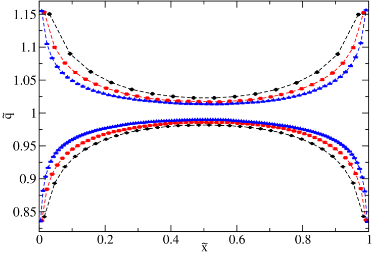
Figure 2: Profiles, eq. (7), at $c_{1,b}=c_{2,b}=1$ and the lattice sizes $L=32$, $64$ and $128$. We plot $\tilde{q}=q(x_{0})/\bar{q}$ as a function of $\tilde{x}=x_{0}/L$ and $\tilde{x}=(x_{0}-L)/L$ for the fine and the coarse lattice, respectively. The curves for the different lattice sizes can be identified by the number of data points. Furthermore $\tilde{q}<1$ for the fine lattice and $\tilde{q}>1$ for the coarse one. The dashed lines should only guide the eye.

We see that there are large corrections at the boundaries. For the fine lattice $q(x_{0})$ is too small and too large for the coarse lattice. This effect only slowly decreases with increasing lattice size. This rather strong deviation from the behavior of the homogeneous system can also be seen clearly in the estimates of $V_{1}$ and $V_{2}$ reported in table 2. We also give the estimates of

$$R_{V}=\frac{V_{1}}{V_{2}}-1$$ (13)

which allows us to monitor the asymmetry between the fine and the coarse lattice.

Table 2: Results for $\bar{\beta}_{1,2}$, $V_{1}$ and $V_{2}$ at $c_{1,b}=c_{2,b}=1$ and $\beta_{c}$. In the last column we give $R_{V}$ as defined in eq. (13).

$L$	$\bar{\beta}_{1,2}$	$V_{1}-\bar{V}$	$V_{2}-\bar{V}$	$R_{V}$
32	0.191000(23)	0.0213(3)	–0.0265(3)	0.0262(2)
64	0.190598(48)	0.0169(8)	–0.0194(7)	0.0200(6)
128	0.190505(25)	0.0121(7)	–0.0147(6)	0.0147(5)

We see that $|V_{1}-\bar{V}|$, $|V_{2}-\bar{V}|$, and $|R_{V}|$ are decreasing rather slowly with increasing lattice size $L$. Fitting with the Ansatz

$$V_{1}-\bar{V}=cL^{-\omega_{V}}$$ (14)

we obtain $\omega_{V}\approx 0.4$. For $V_{2}-\bar{V}$ and $R_{V}$ we get similar results.

It turns out that this deviation from the desired behavior can be lifted to a large extend by tuning $c_{1,b}$ and $c_{2,b}$. We employ the quantities $V_{1}$ and $V_{2}$ to this end. By construction, they are not sensitive to corrections that decay rapidly with increasing distance from the boundary between the fine and the coarse lattice.

First we searched for choices of $c_{1,b}$ and $c_{2,b}$, where $R_{V}$ vanishes. Our simulations show that this is the case for a line in the $(c_{1,b},c_{2,b})$-plane. At the level of the precision of our preliminary study this is the case for e.g. $(c_{1,b},c_{2,b})=(1,0.843)$, $(1.072,0.93)$, $(1.128,1)$. However, it turns out that in general still $V_{1}\approx V_{2}$ deviate from the value obtained for the homogeneous system. For $(c_{1,b},c_{2,b})=(1,0.843)$ we get $V_{1}-\bar{V}=0.0052(3)$, $0.0025(4)$, and $0.0021(6)$ for $L=$ $32$, $64$, and $128$, respectively. On the other hand, for $(c_{1,b},c_{2,b})=(1.128,1)$ we get $V_{1}-\bar{V}=-0.0059(3)$, $-0.0028(4)$, and $-0.0019(5)$ for $L=$ $32$, $64$, and $128$, respectively. For $(c_{1,b},c_{2,b})=(1.072,0.93)$ we find that $V_{1}-\bar{V}$ approximately vanishes.

Motivated by this preliminary study, we systematically searched for the $(c_{1,b},c_{2,b})$, where both $V_{1}-\bar{V}$ and $V_{2}-\bar{V}$ vanish at $\bar{\beta}_{1,2}$. To this end we simulated systems with $L=24$, $32$ and $48$ for various choices of $(c_{1,b},c_{2,b})$ and interpolated $V_{1}-\bar{V}$ and $V_{2}-\bar{V}$ linearly in $(c_{1,b},c_{2,b})$. Our results are summarized in table 3.

Table 3: Estimates of the optimal $(c_{1,b},c_{2,b})$ at $\bar{\beta}_{1,2}$ and $\beta_{1}=\beta_{2}=\beta_{c}$ as a function of the lattice size $L$. We also give the sum and the difference of the optimal $c_{1,b}$ and $c_{2,b}$.

$L$	$c_{1,b}$	$c_{2,b}$	$c_{1,b}+c_{2,b}$	$c_{1,b}-c_{2,b}$
24	1.0685(5)	0.9237(5)	1.9922(8)	0.1448(3)
32	1.0679(6)	0.9233(7)	1.9912(11)	0.1446(3)
48	1.0681(9)	0.9235(12)	1.9916(20)	0.1446(4)

It turns out that the difference $c_{1,b}-c_{2,b}$ has a much smaller error than the sum $c_{1,b}+c_{2,b}$. This might correspond to the fact that for the line where $R_{V}=0$ the difference $c_{1,b}-c_{2,b}$ is roughly constant.

Since the estimates obtained for $L=24$, $32$ and $48$ are consistent within errors, we abstained from studying larger lattice sizes at this point. As our final choice we take

$$(c_{1,b},c_{2,b})=(1.068,0.9234)\;.$$ (15)

We had simulated at $L=24$, $32$ and $48$ at $(c_{1,b},c_{2,b})=(1.068,0.923)$ and $(1.068,0.924)$ with a high statistics of $10^{8}$ measurements or more. In table 4 we interpolate the numerical results to $(c_{1,b},c_{2,b})=(1.068,0.9234)$. Furthermore we report the results of simulations performed directly at $(c_{1,b},c_{2,b})=(1.068,0.9234)$ for $L=64$, $96$ and $128$. For these lattice sizes we performed $94\times 10^{6}$, $61\times 10^{6}$ and $46\times 10^{6}$ measurements, respectively. The simulations of the $L=128$ lattice took about 5.4 years of CPU-time on a single core of a Quad-Core AMD Opteron(tm) 2378 CPU.

Table 4: Results for $\bar{\beta}_{1,2}$, $V_{1}-\bar{V}$ and $V_{2}-\bar{V}$ at the optimal $(c_{1,b},c_{2,b})=(1.068,0.9234)$ at $\beta_{1}=\beta_{2}=\beta_{c}$. For a discussion see the text.

$L$	$\bar{\beta}_{1,2}$	$V_{1}-\bar{V}$	$V_{2}-\bar{V}$
24	0.1858875(47)	0.00010(6)	–0.00000(5)
32	0.1858599(43)	–0.00003(6)	0.00000(6)
48	0.1858328(39)	0.00001(7)	0.00001(6)
64	0.1858187(46)	–0.00002(11)	0.00002(8)
96	0.1858184(45)	–0.00007(13)	0.00000(9)
128	0.1858099(45)	–0.00001(15)	0.00002(13)

We find that for $L=64$, $96$ and $128$ the estimates of $V_{1}-\bar{V}$ and $V_{2}-\bar{V}$ remain consistent with zero. We fitted our data for $\bar{\beta}_{1,2}$ with the Ansatz

$$\bar{\beta}_{1,2}(L)=\bar{\beta}_{1,2}(\infty)+cL^{-\epsilon}\;.$$ (16)

Taking $\epsilon=2$ and the data for $L=48$, $64$, $96$ and $128$ we arrive at $\bar{\beta}_{1,2}(\infty)=0.1858085(39)$, $c=0.054(14)$ and $\chi^{2}$/d.o.f.$=0.36$. In order to check the dependance of the result on $\epsilon$ we repeated the fit with $\epsilon=1.6$. We arrive at $\bar{\beta}_{1,2}(\infty)=0.1858061(45)$, $c=0.013(3)$ and $\chi^{2}$/d.o.f.$=0.38$. Since the estimates of $\bar{\beta}_{1,2}$ obtained for $L=64$, $96$ and $128$ are consistent within errors, it is not surprising that $\bar{\beta}_{1,2}(\infty)$ does not depend strongly on $\epsilon$. As our final estimate we take

$$\bar{\beta}_{1,2}(\infty)=0.185807(6)\;.$$ (17)

where the error that we quote also takes into account the systematic uncertainty of the extrapolation to $L\rightarrow\infty$.

In Fig. 3 we plot $\tilde{q}=q(x_{0})/\bar{q}$, eq. (7), for $(c_{1,b},c_{2,b})=(1.068,0.9234)$, $\beta=0.387721735$ and $\beta_{1,2}=0.185807$. The improvement compared with $(c_{1,b},c_{2,b})=(1,1)$ potted in Fig. 2 is fairly obvious. Starting from a distance of roughly $10$ lattice spacings from the boundary we find that $q(x_{0})$ is consistent, at the level of our statistical accuracy, with the result obtained for the homogeneous system. This observation holds for both the fine as well as for the coarse lattice. We checked also the behavior of $E_{0}(x_{0})$ and $E_{12}(x_{0})$, eqs. (9,10), as a function $x_{0}$. Here we find that starting from a distance of roughly $13$ lattice spacings from the boundary $E_{0}(x_{0})$ and $E_{12}(x_{0})$ are consistent with the results obtained for the homogeneous system.

To be on the safe side, studying properties of the homogeneous system, one should keep at least a distance of $\approx 20$ lattice spacings from the boundary between different lattice spacings.

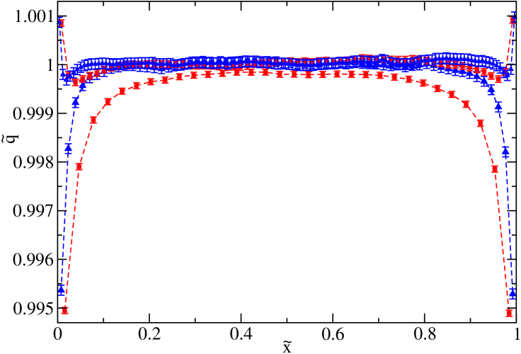
Figure 3: Profiles, eq. (7), at $c_{1,b}=1.068$, $c_{2,b}=0.9234$, $\beta=0.387721735$, $\beta_{1,2}=0.185807$ and the lattice sizes $L=64$ and $128$. We plot $\tilde{q}=q(x_{0})/\bar{q}$ as a function of $\tilde{x}=x_{0}/L$ and $\tilde{x}=(x_{0}-L)/L$ for the fine and the coarse lattice, respectively. The curves for the different lattice sizes can be identified by the number of data points. Furthermore $\tilde{q}<1$ for the fine lattice and $\tilde{q}>1$ for the coarse one. The dashed lines should only guide the eye.

IV.2 Going off-critical

The coupling $\beta_{2}$ in the bulk of the coarse lattice as a function of the coupling $\beta_{1}$ of the fine lattice is chosen such that the bulk correlation length is the same for both parts of the lattice. Hence in terms of the correlation length $\xi$ in units of the respective lattice spacing we get

$$\xi(\beta_{1})=2\xi(\beta_{2})\;.$$ (18)

In the neighborhood of the critical point, the correlation length behaves as

$$\xi(\beta)=\xi_{0}|t|^{-\nu}\;(1+b|t|^{\theta}+ct+d|t|^{\theta^{\prime}}+e|t|^{2\theta}+...)\;,$$ (19)

where $t=\beta_{c}-\beta$ is our definition of the reduced temperature. Here we discuss an improved model which is characterized by $b\approx 0$. Hence, in the following we shall neglect the terms $b|t|^{\theta}$ and $e|t|^{2\theta}$. Note that $\theta^{\prime}=\nu\omega^{\prime}$, where $\omega^{\prime}=1.67(11)$, ref. NewmanRiedel . Hence in the numerical analysis of data for the correlation length it is difficult to disentangle the corrections $ct$ and $d|t|^{\theta^{\prime}}$. After a preliminary study, we realized that for our purpose corrections to scaling can be ignored entirely. Hence we get the linear relation

$$(\beta_{c}-\beta_{2})=(\beta_{c}-\beta_{1})\;2^{1/\nu}\;\;,$$ (20)

where we take $\nu=0.63002$, ref. mycritical . In order to keep things simple, $c_{1,b}$ and $c_{2,b}$ keep their values as determined above at the critical point.

It remains to determine $\bar{\beta}_{1,2}$ as a function of $\beta_{1}$. Analogous to eq. (11) we impose

$$G_{1,2}(L,\beta_{1},\bar{\beta}_{1,2})=\bar{G}(L,\beta_{1}):=\frac{G_{1,2,hom}(L/2,\beta_{2})+G_{1,2,hom}(L,\beta_{1})}{2}\;.$$ (21)

We have simulated $L=24$ and $48$ at one value of $\beta_{1}$ in the high temperature phase and one value of $\beta_{1}$ in the low temperature phase. In order to check the dependance of the result on the difference of these two values of $\beta_{1}$, we simulated $L=32$ at four values of $\beta_{1}$. The corresponding results for the slopes $\Delta\bar{\beta}_{1,2}/\Delta\beta_{1}$ are given in table 5.

Table 5: Results for the slopes $\Delta\bar{\beta}_{1,2}/\Delta\beta_{1}$ at $(c_{1,b},c_{2,b})=(1.068,0.9234)$

$L$	$\beta_{1}$,high	$\beta_{1}$,low	$\Delta\bar{\beta}_{1,2}/\Delta\beta_{1}$
24	0.386	0.39	0.9738(38)
32	0.386	0.3895	0.9706(51)
32	0.387	0.3885	0.9774(68)
48	0.3871	0.3883	0.9663(99)

Within the numerical accuracy we see no non-linearity nor a dependence on $L$. As our final result we take

$$\frac{\mbox{d}\bar{\beta}_{1,2}}{\mbox{d}\beta_{1}}=0.974(10)$$ (22)

at the critical point.

IV.3 Summary of our results

The relation of the bulk coupling on the fine $\beta_{1}$ and the coarse lattice $\beta_{2}$ is given by eq. (20)

$$(\beta_{c}-\beta_{2})=(\beta_{c}-\beta_{1})\;2^{1/\nu}\;\;,$$ (23)

where we take $\beta_{c}=0.387721735$ and $\nu=0.63002$, ref. mycritical . The amplification of the coupling in the layers at the boundary of the coarse and the fine lattice are

$$c_{1,b}=1.068\;\;,\;\;\;\;c_{2,b}=0.9234\;.$$ (24)

For these choices we get for the coupling between the fine and the coarse lattice

$$\beta_{1,2}=0.185807+0.974\;(\beta_{1}-\beta_{c})\;\;.$$ (25)

We recommend to use this approach in a range of couplings give by

$$0.386\lessapprox\beta_{1}\lessapprox 0.391\;.$$ (26)

Note that $\xi_{2nd}(0.386)=12.5747(24)$. For smaller correlation length there is little need to use systems with varying lattice spacing.

V Benchmark: Films with strongly symmetry breaking boundary conditions

We intent to use the results obtained here in the study of the thermodynamic Casimir force between a sphere and a plane. To this end, in the neighborhood of the plane, the lattice spacing $a=1$ is used. Also the sphere should be well inside the part of the lattice with lattice spacing $a=1$. At increasing distances from the plane, larger and larger lattice spacings are used. This way, a semi-infinite system could be approximated at relatively low computational costs. The systematic error that is introduced by the coarsening of the lattice could be controlled by varying the thickness of the sectors of a given lattice spacing, in particular the one next to the plane.

Here, as a benchmark and preliminary step, we study the thermodynamic Casimir force between two plates. This geometry is usually called film geometry. In particular we shall simulate systems with strongly symmetry breaking boundary conditions. This problem has been thoroughly studied. For example, in refs. VaGaMaDi08 ; MHcorrections Monte Carlo simulations of the Ising model on the simple cubic lattice were performed. In refs. MHstrong ; MHcorrections ; myRecent the improved Blume-Capel model on the simple cubic lattice, the model that we consider here, has been studied. Hence accurate numbers to compare with are available. In addition to the thermodynamic Casimir force we determine the magnetization profile. Films with strongly symmetry breaking boundary were also studied for example by using the extended de Gennes-Fisher local-functional method BoUp98 ; BoUp08 ; UpBo13 .

V.1 Thin films with strongly symmetry breaking boundary conditions

We study a lattice of the size $(L_{0}+2)\times L_{1}\times L_{2}$, where $L_{1}=L_{2}=L$ throughout. In $1$- and $2$-direction periodic boundary conditions are imposed. In our convention $x_{0}\in\{0,1,...,L_{0}+1\}$. Strongly symmetry breaking boundary conditions are implemented by fixing the spins at $x_{0}=0$ and $L_{0}+1$ to either $s_{x}=-1$ or $s_{x}=1$. In the case of $(+,+)$ boundary conditions, the spins at both boundaries $x_{0}=0$ and $L_{0}+1$ are fixed to $s_{x}=1$, while for $(+,-)$ boundary conditions, the spins at $x_{0}=0$ are fixed to $s_{x}=1$ and those at $L_{0}+1$ are fixed to $s_{x}=-1$. In order to determine the thermodynamic Casimir force, we simulated two films of the thickness $L_{0,1}=L_{0}+1/2$ and $L_{0,2}=L_{0}-1/2$. In the following $L_{0,2}$ is always a multiple of $4$. In our simulations we used two different lattice spacings only. In particular, we kept the layers $x_{0}=0$, $1$, …, $L_{0,2}/4$ and $x_{0}=3L_{0,2}/4+1$, $3L_{0,2}/4+2$, … $L_{0,i}+1$ as fine lattice. The remaining ones, in the center of the film, are replaced by a coarse lattice with twice the lattice spacing.

The thermodynamic Casimir force per area is defined by

$$\beta F_{Casimir}=-\frac{\partial f_{ex}}{\partial L_{0}}\;\;,$$ (27)

where $f_{ex}=f_{film}-L_{0}f_{bulk}$ is the reduced excess free energy per area of the film of the thickness $L_{0}$ and $f_{film}$ is the reduced free energy per area of the film and $f_{bulk}$ is the reduced free energy density of the bulk system. On the lattice the partial derivative (27) is approximated by a finite difference

$$\frac{\partial f_{ex}}{\partial L_{0}}\approx\Delta f_{ex}$$ (28)

where

$$\Delta f_{ex}(L_{0})=f_{ex}(L_{0}+1/2)-f_{ex}(L_{0}-1/2)\;.$$ (29)

Here, following Hucht Hucht we compute $\Delta f_{ex}$ by integrating the corresponding difference of excess internal energies per area

$$\Delta f_{ex}=-\int_{\beta_{0}}^{\beta}\mbox{d}\tilde{\beta}\Delta E_{ex}$$ (30)

where

$$\Delta E_{ex}(L_{0})=\Delta E(L_{0})-E_{bulk}$$ (31)

where $E_{bulk}$ is the energy density of the bulk system and

$$\Delta E(L_{0})=E(L_{0}+1/2)-E(L_{0}-1/2)$$ (32)

where we define the energy per area of the homogeneous system as

$$E=\frac{1}{L_{1}L_{2}}\sum_{<xy>}\langle s_{x}s_{y}\rangle\;.$$ (33)

Now let us discuss how this approach can be generalized to our system with two different lattice spacings. The partition function takes the form

$$Z=\sum_{\{S\},\{s\}}\exp\left(\beta e_{0}(\{s\})+\sum_{i}(a_{i}+b_{i}\beta)e_{i}(\{S\},\{s\})-D\sum_{x}s_{x}^{2}-D\sum_{X}S_{X}^{2}\right)$$ (34)

where the $\{S\}$ are the spins on the coarse lattice and $\{s\}$ the ones on the fine lattice. The $e_{i}$ correspond to sums in eq. (2). Taking the derivative of the reduced free energy per area with respect to $\beta$ we arrive at

$$\frac{\partial f}{\partial\beta}=-\frac{1}{L_{1}L_{2}}\frac{\partial\ln Z}{\partial\beta}=-\frac{1}{L_{1}L_{2}}\left[\langle e_{0}\rangle+\sum_{i}b_{i}\langle e_{i}\rangle\right]$$ (35)

which means that eq. (33) is generalized to

$$E=\frac{1}{L_{1}L_{2}}\left[\langle e_{0}\rangle+\sum_{i}b_{i}\langle e_{i}\rangle\right]\;\;.$$ (36)

V.2 Numerical results

Here we have repeated a part of the simulations discussed in section 5 of ref. myRecent . The parameters of the simulation are very similar to those of ref. myRecent . In particular we used the exchange cluster algorithm and the improved estimator that is associated with it, to compute $\Delta E$. The implementation of the exchange cluster algorithm for the system with two different lattice spacings and the associated Hamiltonian is straight forward.

Let us first discuss the results obtained for $\Delta E$ for $(+,+)$ boundary conditions. We simulated $(+,+)$ boundary conditions for $(L_{0},L)=(16.5,64)$, $(32.5,128)$, and $(64.5,256)$ at about 100 values of $\beta$ in the neighborhood of the critical point.

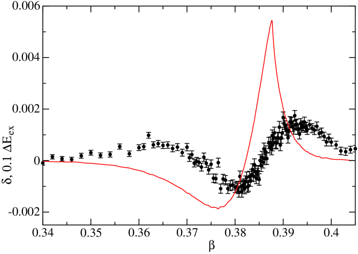
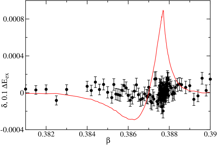
Figure 4: We plot $\delta=\Delta E-\Delta E_{hom}$ for $(+,+)$ boundary conditions as a function of $\beta$. In addition we show as solid red line, $0.1\Delta E_{ex,hom}$. Results for the lattice size $(L_{0},L)=(16.5,64)$ and $(L_{0},L)=(64.5,256)$ are given in the upper and lower part of the figure, respectively.

In the upper part of Fig. 4 we plot the difference $\delta=\Delta E-\Delta E_{hom}$ and $0.1\Delta E_{ex,hom}$ for $L_{0}=16.5$ and $L=64$, where $hom$ indicates the result for the homogeneous system, taken from ref. myRecent . We see that $\delta$ is definitely different from zero for most of the values of $\beta$ that we have simulated at. On the other hand, on average $|\delta|$ is much smaller than $|\Delta E_{ex,hom}|$. Therefore the result that we get for the thermodynamic Casimir force is at least qualitatively correct. Going to larger thicknesses the error due to the coarsening in the center of the film becomes less and less visible. While for $L_{0}=32.5$ still $|\delta|\neq 0$ at the level of our statistical accuracy, for $L_{0}=64.5$ a deviation of $\Delta E$ from $\Delta E_{hom}$ can hardly be seen. See the lower part of Fig. 4.

Let us turn to $(+,-)$ boundary conditions. We simulated films of the thicknesses $L_{0}=16.5$, $32.5$ and $64.5$. For each thickness we simulated at several values of $L$. For example for $L_{0}=16.5$ we studied $L=64$, $128$ and $256$, where $L$ is increased with increasing $\beta$. For a more detailed discussion see ref. myRecent . Our numerical results for $\delta=\Delta E-\Delta E_{hom}$ for $L_{0}=16.5$ and $64.5$ are shown in Fig. 5. For $L_{0}=16.5$ we see a strong deviation of $\Delta E$ from the corresponding result for homogeneous system in the low temperature phase. This deviation is only one order of magnitude smaller than the quantity $\Delta E_{ex,hom}$ that we like to compute. For the thickness $L_{0}=32.5$ the systematic error $\delta$ is still clearly visible and its functional form is similar to that for $L_{0}=16.5$. As for $(+,+)$ boundary conditions, for $L_{0}=64.5$ we find that $\delta$ is essentially consistent with zero at the level of our statistical accuracy.

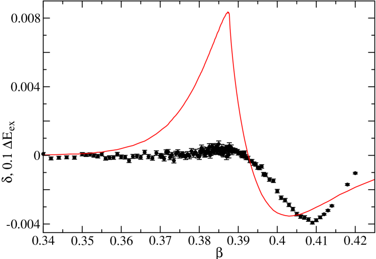
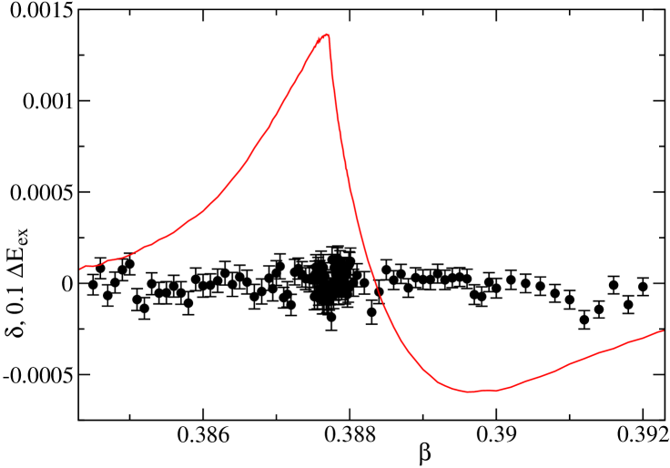
Figure 5: Same as Fig. 4 but for $(+,-)$ instead of $(+,+)$ boundary conditions.

As an additional check, we computed for $L_{0}=64.5$ the integral

$$\Delta=\int_{\beta_{0}}^{\beta}\mbox{d}\tilde{\beta}\;\delta$$ (37)

which gives the error of $\Delta f$. In the case of $(+,+)$ boundary conditions, we find that $\Delta$ is consistent with zero within two standard deviations in the whole range of $\beta$ that we have studied. The some observation holds for $(+,-)$ boundary conditions up to $\beta=0.391$. Then $|\delta|$ is increasing. For $\beta=0.392$ we see a deviation from zero by a little less than three standard deviations.

V.2.1 Magnetization profile

The magnetization profile of the homogeneous system is defined by

$$m(x_{0})=\frac{1}{L_{1}L_{2}}\left\langle\sum_{x_{1},x_{2}}s_{x}\right\rangle\;.$$ (38)

Note that for $(+,\pm)$ boundary conditions

$$m(x_{0})=\pm m(L_{0}+1-x_{0})\;.$$ (39)

For a discussion of the behavior at the critical point see MHstrong and refs. therein. Numerical results are given in section VI. B of MHstrong , see in particular Fig. 1. For simplicity we only discuss the second system that we simulated, since for $L_{0,2}=16$, $32$ and $64$ in contrast to $L_{0,1}=17$, $33$ and $65$, the symmetry (39) is not broken by the coarsening.

Let us first discuss the results obtained for the fine part of the lattice with those for the homogeneous system for the same lattice size. In Fig. 6 we plot the difference

$$\delta m(x_{0})=m(x_{0})-m_{hom}(x_{0})$$ (40)

for $L_{0}=64$ for both $(+,+)$ and $(+,-)$ boundary conditions. For individual values of $\beta$ we can hardly distinguish $\delta m(x_{0})$ from zero. Therefore, we have averaged $\delta m(x_{0})$ over all values $0.3852\leq\beta\leq 0.38792$ we simulated at. This way a small systematic error is revealed.

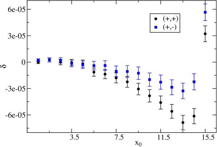
Figure 6: We plot the difference $\delta m(x_{0})$, eq. (40), between the magnetization profiles of the composite and the homogeneous system for both $(+,+)$ and $(+,-)$ boundary conditions and the thickness $L_{0}=64$ at the critical temperature. We averaged $\delta m(x_{0})$ over all values $0.3852\leq\beta\leq 0.38792$ we simulated at.

We also determined $\delta m$ for the thicknesses $L_{0}=16$, $32$. Already here the systematical error is rather small.

For the coarse part of the lattice the comparison is less direct. First one has to rescale the magnetization profile by a factor of $2^{-(1+\eta)/2}$ to compare it with the corresponding profile of the homogeneous system. Moreover, the coarse sites are located at integer values of $x_{0}$, while in our convention the sites of the fine lattice assume half integer values of $x_{0}$. Therefore also an interpolation of the profile is needed for the comparison. Here we do not delve into this direction but simply plot our data. In Fig. 7 we plot the magnetization profile at $\beta=0.387721735$ for $(+,+)$ and $(+,-)$ boundary conditions. We give the results obtained for the homogeneous system and those for the coarse lattice that we have rescaled as discussed above. At least by eye one can only see a deviation in the case of $(+,+)$ boundary conditions at $x_{0}=17$, next to the boundary between parts of the lattice with different lattice spacings. The magnetization on the coarse lattice seems a bit too small compared with the one of the homogeneous lattice.

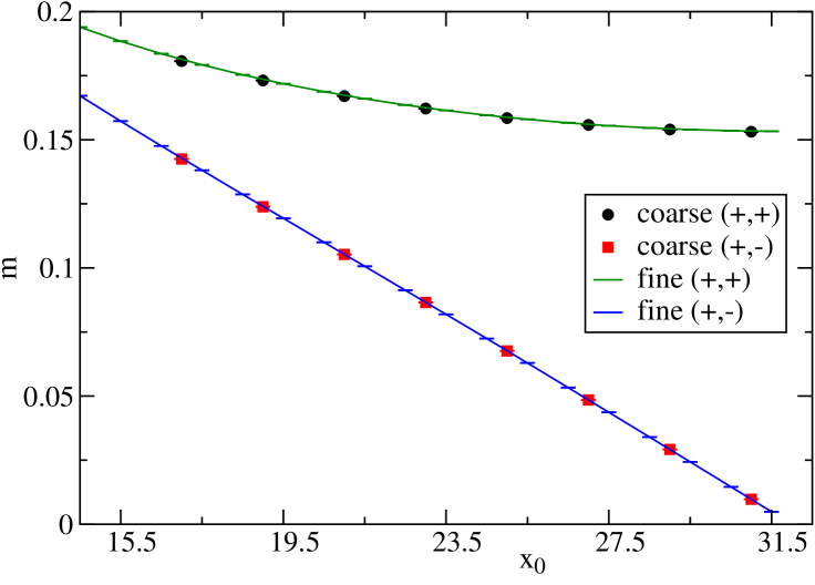
Figure 7: We plot the magnetization profile for both $(+,+)$ and $(+,-)$ boundary conditions and the thickness $L_{0}=64$ at the critical temperature. The data points denoted by “fine” are taken from simulations of the homogeneous system. The data point taken from the coarse part of the composite lattice are rescaled by a factor of $2^{-(1+\eta)/2}$. In the case of the fine lattice, the solid lines should only guide the eye.

VI Conclusions and Outlook

We aim at studying critical phenomena using lattices with adaptive lattice spacing. This should be useful in studies of systems with nontrivial boundary conditions. We are planning to study the thermodynamic Casimir force between a planar and a spherical object or between two spherical objects. In critical phenomena an adaptive grid is difficult to implement, since the field and the couplings rescale nontrivially under a change of the length scale. The present work is a first step in this direction. We consider the universality class of the three-dimensional Ising model. Our starting point is the improved Blume-Capel model on the simple cubic lattice with lattice spacing $a$. The general idea is to replace the sites within certain sectors of the lattice by coarse sites that are separated by a lattice spacing $2a$. This procedure might be iterated to lattice spacings $4a$, $8a$, … . Furthermore these sectors are composed of cubes with faces that are parallel to the lattice-axis. Here we made a first step in this program. In section III we worked out, how two half spaces with lattice spacing $a$ and $2a$, respectively, that are separated by a boundary that is perpendicular to one of the lattice axis, can be coupled consistently. To this end, we used finite size scaling. The boundary between lattice spacing $a$ and $2a$ can be viewed as a defect plane. Following refs. BuEi81 ; DiDiEi83 , there is one relevant perturbation with the RG-exponent $y=y_{t}-1$, where $y_{t}=1/\nu$, associated with it. Hence one would expect that it is sufficient to tune the coupling between the two half spaces. However it turned out that slowly decaying corrections remain. These can be removed by tuning the couplings within the layers next to the boundary. Our final results for the coupling constants are summarized in section IV.3. In a more general scenario we have also edges and corners. These can be regarded as line and point defects, respectively. Following the argument given in the appendix of BuEi81 the RG-eigenvalues are $y_{l}=y_{t}-2=-0.41275(25)$ and $y_{p}=y_{t}-3=-1.41275(25)$, respectively. Hence both perturbations of the fixed point are irrelevant. Therefore in principle no additional tuning of couplings at the edges and corners is needed. However the absolute value of $y_{l}$ is rather small and hence still tuning of a coupling at the edges seems to be beneficial. It remains to be worked out which coupling could be tuned and which observables could be used to tune it.

In order to benchmark our results we simulated films with strongly symmetry breaking boundary conditions. We replaced half of the sites, located in the center of the film, by coarse sites. We computed the magnetization profile and the partial derivative of the internal energy with respect to the thickness of the film. This quantity is used to determine the thermodynamic Casimir force. For the largest thickness $L_{0}=64.5a$ that we have simulated, at the level of our statistical accuracy, the numerical results can hardly be discriminated from those obtained by simulating a system with a unique lattice spacing.

VII Acknowledgement

This work was supported by the DFG under the grant No HA 3150/3-1.

References

- (1) M. Krech, Casimir Effect in Critical Systems (World scientific, Singapure, 1994).
- (2) M. Krech, Fluctuation-induced forces in critical fluids, J. Phys.: Condens. Matter 11, R391 (1999).
- (3) J. G. Brankov, D. M. Dantchev, and N. S. Tonchev, Theory of Critical Phenomena in Finite-Size Systems – Scaling and Quantum effects (World scientific, Singapure, 2000).
- (4) A. Gambassi, The Casimir effect: from quantum to critical fluctuations, [arXiv:0812.0935], J. Phys. Conf. Series 161, 012037 (2009).
- (5) M. Hasenbusch, Thermodynamic Casimir Forces between a Sphere and a Plate: Monte Carlo Simulation of a Spin Model, [arXiv:1210.3961], Phys. Rev. E 87, 022130 (2013).
- (6) T. G. Mattos, L. Harnau, and S. Dietrich, Many-body effects for critical Casimir forces The Journal of Chemical Physics 138, 074704 (2013).
- (7) T. G. Mattos, L. Harnau, and S. Dietrich, Three-body critical Casimir forces [arXiv:1408.7081].
- (8) T. W. Burkhardt and E. Eisenriegler, Critical phenomena near surfaces and defect lines, Phys. Rev. B 24, 1236 (1981).
- (9) H. W. Diehl, S. Dietrich, and E. Eisenriegler, Universality, irrelevant surface operators, and corrections to scaling in systems with free surfaces and defect planes, Phys. Rev. B 27, 2937 (1983).
- (10) M. Hasenbusch, Thermodynamic Casimir Effect in Films: the Exchange Cluster Algorithm, [arXiv:1410.7161].
- (11) Y. Deng and H. W. J. Blöte, Constraint tricritical Blume-Capel model in three dimensions, Phys. Rev. E 70, 046111 (2004).
- (12) M. Hasenbusch, A Finite Size Scaling Study of Lattice Models in the 3D Ising Universality Class, [arXiv:1004.4486], Phys. Rev. B 82, 174433 (2010).
- (13) U. Wolff, Collective Monte Carlo Updating for Spin Systems, Phys. Rev. Lett. 62, 361 (1989).
- (14) M. Hasenbusch, Universal amplitude ratios in the 3D Ising Ising Universality Class, [arXiv:1004.4983], Phys. Rev. B 82, 174434 (2010).
- (15) K. E. Newman and E. K. Riedel, Critical exponents by the scaling-field method: The isotropic -vector model in three dimensions, Phys. Rev. B 30, 6615 (1984).
- (16) O. Vasilyev, A. Gambassi, A. Maciołek, and S. Dietrich, Universal scaling functions of critical Casimir forces obtained by Monte Carlo simulations, [arXiv:0812.0750], Phys. Rev. E 79, 041142 (2009).
- (17) M. Hasenbusch, Thermodynamic Casimir effect: Universality and Corrections to Scaling, [arXiv:1202.6206], Phys. Rev. B 85, 174421 (2012).
- (18) M. Hasenbusch, Thermodynamic Casimir effect for films in the 3D Ising universality class: Symmetry breaking boundary conditions, [arXiv:1005.4749], Phys. Rev. B 82, 104425 (2010).
- (19) Z. Borjan and P. J. Upton, Order-Parameter Profiles and Casimir Amplitudes in Critical Slabs, Phys. Rev. Lett. 81, 4911 (1998).
- (20) Z. Borjan and P. J. Upton, Off-Critical Casimir Effect in Ising Slabs with Symmetric Boundary Conditions in , [arXiv:0804.2340], Phys. Rev. Lett. 101, 125702 (2008).
- (21) P. J. Upton and Z. Borjan, Off-critical Casimir effect in Ising slabs with antisymmetric boundary conditions in Phys. Rev. B 88, 155418 (2013).
- (22) A. Hucht, Thermodynamic Casimir Effect in 4He Films near : Monte Carlo Results, [arXiv:0706.3458], Phys. Rev. Lett. 99, 185301 (2007).