High-order fractional-compact finite difference method for Riesz spatial telegraph equation

Abstract

In this paper, we establish even order fractional-compact numerical differential formulas (4th-order, …, 10th-order) for Riesz derivatives by using the symmetrical fractional centred difference operator. Then we apply the derived 4th-order algorithm to the Riesz spatial telegraph equation. We carefully study the stability and convergence by the energy method, and show that convergence orders in temporal and spatial directions are both 4th order. Numerical experiments are displayed which support the fractional-compact numerical differentiation formulas for Riesz derivatives and the Riesz spatial telegraph equation.

Key words: Riesz derivative; Fractional-compact numerical differential formula; Riesz spatial telegraph equation; Stability and convergence.

AMS subject classifications: 65M06, 65M12

1 Introduction

In recent decades, fractional calculus (i.e., fractional integrals and fractional derivatives) have attracted increasing interest mainly due to its potential applications in various realms of science and engineering [23, 25, 32].

As far as we know, there are more than six kinds of fractional derivatives. Usually, the time-fractional derivatives are given in the Caputo or Riemann-Liouville sense. As for the space-fractional derivative, it is commonly defined as an operator inverse to the Riesz potential and is referred to as the Riesz fractional derivative [2, 32]. Because the exact solutions of the most fractional differential equations cannot be analytically obtained, numerical methods for these equations are becoming more and more necessary and important. Generally speaking, the first step to solve fractional differential equations is how to approximate the fractional derivatives. For Caputo derivatives, the commonly approximation scheme is $L_{1}$ formula with convergence order $\mathcal{O}(\tau^{2-\alpha})$ for $0<\alpha<1$ [28] (page 140) and [19]. In [20], Li et. al., proposed several kinds of high-order numerical schemes based on the quadratic interpolation methods, then applied some of them to the fractional ordinary differential equations. Cao and Xu [5] further developed a numerical scheme with convergence order $(3+\alpha)$ for $0<\alpha<1$ and order 4 for $\alpha>1$ under suitable smooth conditions. Recently, a $(3-\alpha)$-th order scheme was proposed by Gao et. al., and they used it to solve time fractional differential equations, but they didn’t give the stability and convergence analysis for the corresponding difference scheme [15]. Almost at the same time, Li et al., [22] also independently constructed a $(3-\alpha)$-th order numerical approximation formula, meanwhile they constructed two unconditionally stable difference schemes for time fractional advection-dispersion equation with convergence orders $\mathcal{O}(\tau^{3-\alpha}+h^{2})$ and $\mathcal{O}(\tau^{3-\alpha}+h^{4})$, where the rigorous theoretical analysis was displayed. More detailed introduction in this respect can be found in [23].

For Riemann-Liouville derivatives, they are often discretized by the standard Grünwald-Letnikov formula. Such schemes have first order accuracy if the homogeneous initial conditions are satisfied. However, they are not numerically stable. To overcome this defect, Meerscharet and Tadjeran firstly proposed the so-called shifted Grünwald-Letnikov formula still with first order accuracy [24]. In [36], Tian, et.al., got a class of second order difference schemes by combining different weights and shifted Grünwald-Letnikov difference operators, the corresponding third order quasi-compact difference schemes were proposed in [41]. Wang and Vong also developed a second order difference scheme and applied it to the modified fractional anomalous subdiffusion equation [37]. In addition, fast numerical algorithms for spatial fractional partial differential equations with the Riemann-Liouville derivatives (or the Riesz derivatives) attract researchers’ interest [38, 39].

In general, Lévy flights and Lévy walks are used to model anomalous diffusion, which is governed by rare but extremely large jumps of diffusing particles [3]. In Lévy walks, the time of travel is proportional to the total path length if the walkers travel with constant velocity. This leads to the function with respect to time for the mean-square displacement exists and its grows much faster than the linear case. Consequently, This property makes Lévy walks applicable for modeling superdiffusion. However, the time evolution of Lévy flights is simpler than that of Lévy walks. Hence, the former is better than the latter commonly used in real life applications. In the continuous limit, Lévy flight process is described by the superdiffusion equation, which includes the first order derivative with respect to time and fractional Riesz operator with respect to spatial coordinates [25], that is to say, the Riesz space-fractional derivative has been shown to be relevant for anomalous diffusion models. In Riesz spatial fractional differential equations, the order of the Riesz derivative often belongs to $(1,2)$. Such a Riesz derivative defined in spatial domain, which well characterize the heterogeneity and long-range actions in space, is similar to the Laplace operator $\Delta$ in the typical partial differential equations. For the moment, as to the numerical algorithms for Riesz derivatives, the above numerical methods can be applied directly to them due to the Riesz derivatives being the special linear combinations of the left and right Riemann-Liouville derivatives. Later, Ortigueita defined a fractional centred difference operator deal with the Riesz derivatives [26]. Çelik and Duman [6] showed that the fractional centred difference operator has second order accuracy, and they used it to solve the Riesz spatial diffusion equation on a finite domain. Shen et al., [33] also applied the above operator to the Riesz space fractional advection diffusion equation. Hence, to the best of our knowledge, it seems that the convergence orders of the existing numerical approximation formulas for Riesz derivatives are more lower and most of them are no more than 4, except for the results are given by Ding et al. in [10, 11], who established a series of higher-order numerical algorithms and also applied them to the Riesz type fractional partial differential equations, where the stability and convergence were studied in details. Note that the nonlocal properties of fractional operators, using the high-order numerical algorithms for space fractional differential equations leads to almost the same computational cost with low-order ones due to the corresponding derived matrixes are all full and have almost the same structures. However, the convergence order (or accuracy) is greatly improved. So the development of the high-order numerical approximation formulas for Riesz derivatives have attracted utmost interest in recent years. In this paper, we continue to study the numerical methods for Riesz derivatives whose order lies in $(1,2)$. We establish the 4th-order, 6th-order, 8th-order, and 10th-order schemes for approximating Riesz derivatives (the 2nd-order case was displayed in [6]), and named them as the fractional-compact numerical differential formulas. They can be smoothly applied to Riesz spatial differential equations. For convenience, we only use the fractional-compact 4th-order algorithm to solve Riesz spatial telegraph equation. The other order approximations can be similarly applied, so are omitted here.

The reminder of the paper is constructed as follows. In Section 2, we establish even order approximation formulas (from 4th-order to 10th-order) for Riesz derivatives and study some interesting properties of the coefficients in the fractional centred difference operator. A temporal compact and spatial fractional-compact difference scheme for the Riesz spatial telegraph equation is proposed in Section 3, where the stability and convergence of the developed difference scheme is also analysed. Several numerical examples are given in Section 4 to confirm the convergent orders of the proposed numerical formulas. We conclude this paper with some remarks in the last section.

2 The fractional-compact numerical formulas for Riesz derivatives

Firstly, we introduce the definition of the Riesz derivative and the corresponding result.

Definition 1. The $\alpha$-order Riesz derivative of function $u(x,t)$ with respect to $x$ in real line for $1<\alpha<2$ is defined as [32]

$$\begin{array}[]{lll}\displaystyle\frac{\partial^{\alpha}u(x,t)}{\partial{|x|^{\alpha}}}&=&\displaystyle-\kappa_{\alpha}\left(\,{}_{RL}D_{-\infty,x}^{\alpha}+\,_{RL}D_{x,+\infty}^{\alpha}\right)u(x,t)\vspace{0.2 cm}\\ &=&\displaystyle-\frac{\kappa_{\alpha}}{\mathrm{\Gamma}(2-\alpha)}\frac{\partial^{2}}{\partial{x^{2}}}\int_{-\infty}^{+\infty}\frac{u(\eta,t)}{|x-\eta|^{\alpha-1}}\mathrm{d}\eta,\end{array}$$

where $\displaystyle\kappa_{\alpha}=\displaystyle\frac{1}{2}\sec\left(\frac{\pi\alpha}{2}\right)$, $\,{}_{RL}D_{-\infty,x}^{\alpha}$ and $\,{}_{RL}D_{x,+\infty}^{\alpha}$ are the left and right Riemann-Liouville derivatives with following forms

$$\,{}_{RL}D_{-\infty,x}^{\alpha}u(x,t)=\frac{1}{\mathrm{\Gamma}(2-\alpha)}\frac{\partial^{2}}{\partial{x^{2}}}\int_{-\infty}^{x}\frac{u(\eta,t)}{(x-\eta)^{\alpha-1}}\mathrm{d}\eta,\vspace{0.3cm}\\$$

and

$$\,{}_{RL}D_{x,+\infty}^{\alpha}u(x,t)=\frac{1}{\mathrm{\Gamma}(2-\alpha)}\frac{\partial^{2}}{\partial{x^{2}}}\int_{x}^{+\infty}\frac{u(\eta,t)}{(\eta-x)^{\alpha-1}}\mathrm{d}\eta.$$

Here, $\mathrm{\Gamma}(\cdot)$ is the Euler’s Gamma function,

$$\begin{array}[]{lll}\displaystyle\mathrm{\Gamma}(\beta)=\int_{0}^{\infty}\exp(-t)t^{\beta-1}\mathrm{d}t,\;\;\beta>0.\end{array}$$

The following function $\psi$ associated with Gamma function [17] will be used later,

$$\begin{array}[]{lll}\displaystyle\psi(\beta)=\frac{\mathrm{\Gamma}^{\prime}(\beta)}{\mathrm{\Gamma}(\beta)}=-\gamma+\int_{0}^{\infty}\frac{\exp(-t)-\exp(-\beta t)}{1-\exp(-t)}\mathrm{d}t,\end{array}$$

where $\gamma=0.57721\cdots$ is Euler’s constant.

Lemma 1. Let $\alpha>0$, $u(x,t)\in L_{1}({\mathrm{R}})$ with respect to $x$, then the Fourier transform of Riesz derivative is given by [30],

$$\begin{array}[]{lll}\displaystyle\mathscr{F}_{x}\left\{\frac{\partial^{\alpha}u(x,t)}{\partial{|x|^{\alpha}}};\omega\right\}=-|\omega|^{\alpha}\hat{u}(\omega,t),\end{array}$$

where $\hat{u}(\omega,t)$ denotes the Fourier transform of function $u(x,t)$ with respect to $x$, i.e.,

$$\hat{u}(\omega,t)=\mathscr{F}_{x}\left\{u(x,t);\omega\right\}=\int_{\mathbb{R}}\exp\left(-\mathrm{i}\omega x\right)u(x,t)\mathrm{d}x,\;\;\mathrm{i}^{2}=-1.$$

We next introduce the fractional centered difference operator proposed by Ortigueira for $\alpha>-1$ [26],

$$\begin{array}[]{lll}\displaystyle\Delta_{h}^{\alpha}u(x,t)=\sum\limits_{k=-\infty}^{\infty}g_{k}^{(\alpha)}u(x-kh,t).\end{array}$$

It is shown that for $1<\alpha<2$, then one has

$$\begin{array}[]{lll}\displaystyle\lim_{h\rightarrow 0}\left(-\frac{\Delta_{h}^{\alpha}u(x,t)}{h^{\alpha}}\right)=\lim_{h\rightarrow 0}\left(-\frac{1}{h^{\alpha}}\sum\limits_{k=-\infty}^{\infty}g_{k}^{(\alpha)}u(x-kh,t)\right)=\frac{\partial^{\alpha}u(x,t)}{\partial{|x|^{\alpha}}}.\end{array}$$

where $g_{k}^{(\alpha)}=\frac{(-1)^{k}\mathrm{\Gamma}(\alpha+1)}{\mathrm{\Gamma}\left(\frac{\alpha}{2}-k+1\right)\mathrm{\Gamma}\left(\frac{\alpha}{2}+k+1\right)}$, $h$ is the spatial stepsize.

In fact, the above fractional centered difference operator can be regarded as the generalization of the second order centered difference operator, i.e.,

$$\begin{array}[]{lll}\displaystyle\lim_{\alpha\rightarrow 2}\Delta_{h}^{\alpha}u(x,t)={u(x-h,t)-2u(x,t)+u(x+h,t)}.\end{array}$$

In [26], it was pointed out that the generating function associated with coefficients $\displaystyle{g}_{{}_{k}}^{(\alpha)}$ in equ. (3) is $\left|2\sin\left(\frac{\omega h}{2}\right)\right|^{\alpha}$, i.e.,

$$\begin{array}[]{rrr}\displaystyle\left|2\sin\left(\frac{\omega h}{2}\right)\right|^{\alpha}=\sum\limits_{k=-\infty}^{\infty}{g}_{{}_{k}}^{(\alpha)}\exp(\mathrm{i}k\omega h).\end{array}$$

By simple calculations, one has following recursive formula,

$$\begin{array}[]{rrr}\displaystyle{g}_{{}_{0}}^{(\alpha)}=\frac{\mathrm{\Gamma}(\alpha+1)}{\mathrm{\Gamma}^{2}\left(\frac{\alpha}{2}+1\right)}>0,\;\;{g}_{{}_{k}}^{(\alpha)}=\left(1-\frac{\alpha+1}{\frac{\alpha}{2}+k}\right){g}_{{}_{k-1}}^{(\alpha)}<0,\;k=\pm 1,\pm 2,\ldots.\end{array}$$

Noticing $0<1-\frac{\alpha+1}{\frac{\alpha}{2}+k}<1$ for $k\geq 2$ and $1-\frac{\alpha+1}{\frac{\alpha}{2}+k}>1$ for $k\leq-1$, then for fixed $\alpha\in(1,2)$ one has

$$\begin{array}[]{rrr}\displaystyle{g}_{{}_{k}}^{(\alpha)}>{g}_{{}_{k-1}}^{(\alpha)}>\cdots>{g}_{{}_{k-s}}^{(\alpha)}>\cdots,\;k=2,3,\ldots,\;s\geq 1,\;k-s\geq 1,\end{array}$$

and

$$\begin{array}[]{rrr}\displaystyle{g}_{{}_{k}}^{(\alpha)}<{g}_{{}_{k-1}}^{(\alpha)}<\cdots<{g}_{{}_{k-s}}^{(\alpha)}<\cdots,\;k=-1,-2,\ldots,\;s\leq 1,\;k-s\leq-2.\end{array}$$

On the other hand, if we fix $k\geq 0$, then we discuss the relationships between $\alpha$ and ${g}_{k}^{(\alpha)}$ for the fixed $k$. Here, we plot the figures of the coefficients ${g}_{k}^{(\alpha)}$, $k=0,1,\ldots,5$. From Figs. 2.1–2.3, one can see that ${g}_{k}^{(\alpha)}$, $k=0,2,3,4,5$ increase with respect to $\alpha\in(1,2)$, ${g}_{1}^{(\alpha)}$ decrease for $\alpha\in(1,2)$. The proof will be given later on. Next, some important properties of these coefficients are also studied which are useful for stability and convergence analysis in some places.

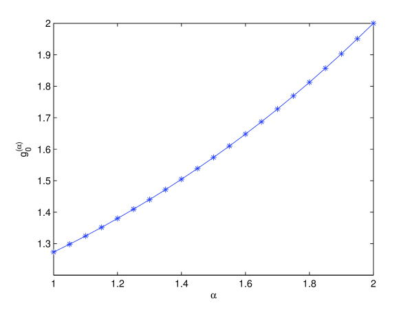
Figure 2.1: The relationship between $g_{0}^{(\alpha)}$ and $\alpha\in(1,2)$.

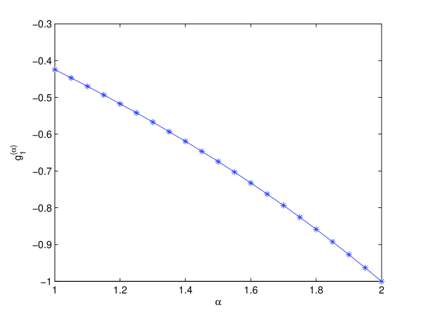
Figure 2.2: The relationship between $g_{1}^{(\alpha)}$ and $\alpha\in(1,2)$.

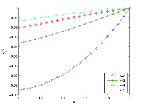
Figure 2.3: The relationship between $g_{k}^{(\alpha)}$ and $\alpha\in(1,2)$, $k=2,3,4,5$.

Theorem 1. If $1<\alpha<2$, then the coefficients $g_{k}^{(\alpha)}$ satisfy the following properties.

$$\begin{array}[]{lll}\displaystyle\mathrm{(i)}\;\;\textit{Boundedness:}\;\;S(\alpha)\left(\frac{\alpha+4}{\alpha+2k}\right)^{2(\alpha+1)}<\left|\right.{g}_{{}_{k}}^{(\alpha)}\left|\right.<S(\alpha)\left(\frac{\alpha+6}{\alpha+2(k+1)}\right)^{\alpha+1},\vspace{0.2 cm}\\ \;\;k\geq 3,\displaystyle\;\;\textmd{where}\;\;S(\alpha)=-\frac{\mathrm{\Gamma}(\alpha+1)}{\mathrm{\Gamma}(\frac{\alpha}{2}-1)\mathrm{\Gamma}(\frac{\alpha}{2}+3)};\vspace{0.3 cm}\\ \displaystyle\mathrm{(ii)}\;\;\textit{Boundedness\; of\; finite\; summations:}\vspace{0.2 cm}\\ \displaystyle P_{1}(m,n,\alpha)\frac{\left(\alpha+4\right)^{2(\alpha+1)}}{2(2\alpha+1)}<\sum\limits_{k=n}^{m}\left|\right.{g}_{{}_{k}}^{(\alpha)}\left|\right.<P_{2}(m,n,\alpha)\frac{\left(\alpha+6\right)^{\alpha+1}}{2\alpha},\;\;n\geq 3,\vspace{0.2 cm}\\ \displaystyle where\;\;P_{1}(m,n,\alpha)=-S(\alpha)\left[(\alpha+2n)^{-(2\alpha+1)}-(\alpha+2m+2)^{-(2\alpha+1)}\right],\;and\vspace{0.2 cm}\\ P_{2}(m,n,\alpha)=-S(\alpha)\left[(\alpha+2n)^{-\alpha}-(\alpha+2m+2)^{-\alpha}\right];\vspace{0.2 cm}\displaystyle\\ \displaystyle\mathrm{(iii)}\;\;\textit{Boundedness\; of\; infinite\; summations:}\vspace{0.2 cm}\\ \displaystyle Q_{1}(n,\alpha)\frac{\left(\alpha+4\right)^{2(\alpha+1)}}{2(2\alpha+1)}<\sum\limits_{k=n}^{\infty}\left|\right.{g}_{{}_{k}}^{(\alpha)}\left|\right.<Q_{2}(n,\alpha)\frac{\left(\alpha+6\right)^{\alpha+1}}{2\alpha},\;\;n\geq 3,\vspace{0.2 cm}\\ \displaystyle where\;\;Q_{1}(n,\alpha)=\frac{-S(\alpha)}{(\alpha+2n)^{2\alpha+1}},\;\;and\;\;Q_{2}(n,\alpha)=\frac{-S(\alpha)}{(\alpha+2n)^{\alpha}};\vspace{0.2 cm}\\ \displaystyle\mathrm{(iv)}\;\;\textit{Boundedness\; of \;two-sided\; infinite\; summations:}\\ \displaystyle\frac{2^{1+\alpha}}{(1+\alpha)\pi}\leq\sum\limits_{k=-\infty,k\neq 0}^{\infty}\left|\right.{g}_{{}_{k}}^{(\alpha)}\left|\right.\leq\frac{2^{1+\alpha}}{\pi};\vspace{0.2 cm}\\ \displaystyle\mathrm{(v)}\;\;\textit{Monotonicity\; with\; respect\; to\;$\alpha$:}\vspace{0.2 cm}\\ \displaystyle\textit{If}\;1\leq\alpha_{1}<\alpha_{2}\leq 2,then\;{g}_{{}_{k}}^{(\alpha_{1})}<{g}_{{}_{k}}^{(\alpha_{2})}\;for\;k\neq 1\;and\;\;{g}_{{}_{k}}^{(\alpha_{1})}>{g}_{{}_{k}}^{(\alpha_{2})}\;for\;k=1.\end{array}$$

Proof. See Appendix I for details. $\blacksquare$

In the following, we construct even order fractional-compact numerical differential formulas for Riesz derivatives.

Theorem 2. Suppose that $\displaystyle u(x,t)\in C^{[\alpha]+2n+1}({\mathrm{R}})$ with respect to $x$ and all the derivatives of $u(x,t)$ with respect to $x$ up to order $[\alpha]+2n+2$ exist and belong to $\displaystyle L_{1}(\mathrm{R})$. Then the following estimate holds,

$$\begin{array}[]{rrr}\displaystyle\frac{\partial^{\alpha}u(x,t)}{\partial{|x|^{\alpha}}}=\left(\delta_{x}^{0}-b_{n-1}\delta_{x}^{2n-2}\right)^{-1}\left(\sum\limits_{\ell=0}^{n-2}b_{\ell}\,\delta_{x}^{2\ell}\right)\left(-\frac{\Delta_{h}^{\alpha}u(x,t)}{h^{\alpha}}\right)+\mathcal{O}(h^{2n}),\\ \;n\in\mathrm{N}^{+},\end{array}$$

where

$$\begin{array}[]{lll}\displaystyle\frac{\Delta_{h}^{\alpha}u(x,t)}{h^{\alpha}}=\frac{1}{h^{\alpha}}\sum\limits_{k=-\infty}^{\infty}g_{k}^{(\alpha)}u(x-kh,t),\end{array}$$

and

$$\begin{array}[]{lll}\displaystyle\delta_{x}^{2\ell}u(x_{j},t)=\sum\limits_{s=0}^{2\ell}(-1)^{s}\dbinom{2\ell}{s}u(x_{\ell+j-s},t),\;\;\ell\geq 0,\end{array}$$

specifically, $\delta_{x}^{0}$ is the identity operator with respect to spatial variable $x$, i.e., $\delta_{x}^{0}u(x_{j},t)=u(x_{j},t).$

Here, the coefficients $b_{\ell}\;\left(\ell=0,1,\ldots,n-2\right)$ satisfy the following equation

$$\begin{array}[]{lll}\displaystyle\sum\limits_{\ell=0}^{n-2}b_{\ell}\left(2\sum\limits_{s=0}^{\ell-1}\sum\limits_{q=0}^{n-1}\sum\limits_{p=0}^{n-1-q}\frac{(-1)^{s+q}(\ell-s)^{2q}\dbinom{2\ell}{s}a_{p}}{(2q)!}\left|\omega h\right|^{2(p+q)}\right.\\ \left.\displaystyle+(-1)^{\ell}\dbinom{2\ell}{\ell}\sum\limits_{p=0}^{n-1}a_{p}\left|\omega h\right|^{2p}\right)\\ \displaystyle=1-b_{n-1}\left(\sum\limits_{s=0}^{n-2}(-1)^{s}\dbinom{2n-2}{s}\frac{2(n-1-s)^{2n-2}}{(2n-2)!}\right)(-1)^{n-1}\left|\omega h\right|^{2n-2},\end{array}$$

and $a_{p}\;(p=0,1,\ldots)$ satisfy the equation

$$\begin{array}[]{lll}\displaystyle\sum\limits_{p=0}^{\infty}a_{p}\left|\omega h\right|^{2p}&=&\displaystyle\left|\frac{2\sin\left(\frac{\omega h}{2}\right)}{\omega h}\right|^{\alpha}=\left[1-\frac{\alpha}{24}|\omega h|^{2}+\left(\frac{1}{1920}+\frac{\alpha-1}{1152}\right)\alpha|\omega h|^{4}\right.\vspace{0.3cm}\\ &&\displaystyle\left.-\left(\frac{1}{322560}+\frac{\alpha-1}{46080}+\frac{(\alpha-1)(\alpha-2)}{82944}\right)\alpha|\omega h|^{6}+\cdots\right].\end{array}$$

Proof. If $n=1$, then equation (4) is reduced to the 2nd-order scheme which was reported in [6]

$$\begin{array}[]{lll}\displaystyle\frac{\partial^{\alpha}u(x)}{\partial{|x|^{\alpha}}}=-\frac{\Delta_{h}^{\alpha}u(x,t)}{h^{\alpha}}+\mathcal{O}(h^{2}).\end{array}$$

The case $n=2$ was already mentioned in [11], here we will further study it and discuss its application in the next section.

Let

$$\begin{array}[]{lll}\displaystyle\mathcal{K}_{n}:=\left(\delta_{x}^{0}-b_{n-1}\delta_{x}^{2n-2}\right),\;\;\;\mathcal{L}_{n}:=\sum\limits_{\ell=0}^{n-2}b_{\ell}\,\delta_{x}^{2\ell},\;\;n\geq 2.\end{array}$$

Taking the Fourier transform to $\mathcal{K}_{n}\frac{\partial^{\alpha}u(x,t)}{\partial{|x|^{\alpha}}}$ gives

$$\begin{array}[]{lll}&&\displaystyle\mathscr{F}_{x}\left\{\mathcal{K}_{n}\frac{\partial^{\alpha}u(x,t)}{\partial{|x|^{\alpha}}};\omega\right\}=\displaystyle\mathscr{F}_{x}\left\{\left(\delta_{x}^{0}-b_{n-1}\delta_{x}^{2n-2}\right)\frac{\partial^{\alpha}u(x,t)}{\partial{|x|^{\alpha}}};\omega\right\}\vspace{0.2cm}\\ &=&\displaystyle-|\omega|^{\alpha}\left(1-b_{n-1}\left(\sum\limits_{s=0}^{n-2}(-1)^{s}\dbinom{2n-2}{s}\frac{2(n-1-s)^{2n-2}}{(2n-2)!}(-1)^{n-1}|\omega|^{2n-2}h^{2n-2}\right.\right.\vspace{0.2 cm}\\ &&\displaystyle\left.\left.+(-1)^{n}|\omega|^{2n}\mathcal{O}(h^{2n})\right)\right)\widehat{u}(\omega,t),\end{array}$$

by using Lemma 1 and the following Taylor series expansion

$$\begin{array}[]{lll}\displaystyle\delta_{x}^{2n-2}u(x,t)&=&\displaystyle\sum\limits_{s=0}^{2n-2}(-1)^{s}\dbinom{2n-2}{s}u(x+(n-1-s)h,t)\vspace{0.2 cm}\\ &=&\displaystyle\sum\limits_{s=0}^{n-2}(-1)^{s}\dbinom{2n-2}{s}\left(\frac{2(n-1-s)^{2n-2}}{(2n-2)!}\frac{\partial^{2n-2}u(x,t)}{\partial x^{2n-2}}\right)h^{2n-2}\vspace{0.2 cm}\\ &&\displaystyle+\frac{\partial^{2n}u(x,t)}{\partial x^{2n}}\mathcal{O}(h^{2n}).\end{array}$$

Similarly, we also have

$$\begin{array}[]{lll}&&\displaystyle\mathscr{F}_{x}\left\{\mathcal{L}_{n}\left(-\frac{\Delta_{h}^{\alpha}u(x,t)}{h^{\alpha}}\right);\omega\right\}=-\displaystyle\mathscr{F}_{x}\left\{\frac{1}{h^{\alpha}}\left(\sum\limits_{\ell=0}^{n-2}b_{\ell}\,\delta_{x}^{2\ell}\right)\sum\limits_{k=-\infty}^{\infty}g_{k}^{(\alpha)}u(x-kh);\omega\right\}\vspace{0.2cm}\\ &=&-\displaystyle\mathscr{F}_{x}\left\{\frac{1}{h^{\alpha}}\left(\sum\limits_{\ell=0}^{n-2}b_{\ell}\sum\limits_{k=-\infty}^{\infty}g_{k}^{(\alpha)}\sum\limits_{s=-\ell}^{\ell}(-1)^{\ell-|s|}\dbinom{2\ell}{\ell-|s|}u(x-(k+s)h)\right);\omega\right\}\vspace{0.2cm}\\ &=&-\displaystyle\frac{1}{h^{\alpha}}\left(\sum\limits_{\ell=0}^{n-2}b_{\ell}\sum\limits_{s=-\ell}^{\ell}(-1)^{\ell-|s|}\dbinom{2\ell}{\ell-|s|}e^{\mathrm{i}s\omega h}\right)\sum\limits_{k=-\infty}^{\infty}g_{k}^{(\alpha)}e^{\mathrm{i}k\omega h}\widehat{u}(\omega,t)\vspace{0.2cm}\\ &=&-\displaystyle\frac{1}{h^{\alpha}}\left(\sum\limits_{\ell=0}^{n-2}b_{\ell}\left(\sum\limits_{s=0}^{\ell-1}2(-1)^{s}\dbinom{2\ell}{s}\cos((\ell-s)\omega h)+(-1)^{\ell}\dbinom{2\ell}{\ell}\right)\right)\vspace{0.2cm}\\ &&\displaystyle\times\sum\limits_{k=-\infty}^{\infty}g_{k}^{(\alpha)}e^{\mathrm{i}k\omega h}\widehat{u}(\omega,t)\vspace{0.2cm}\\ &=&-\displaystyle\frac{1}{h^{\alpha}}\left(\sum\limits_{\ell=0}^{n-2}b_{\ell}\left(\sum\limits_{s=0}^{\ell-1}2(-1)^{s}\dbinom{2\ell}{s}\sum\limits_{q=0}^{\infty}(-1)^{q}\frac{((\ell-s)\omega h)^{2q}}{(2q)!}+(-1)^{\ell}\dbinom{2\ell}{\ell}\right)\right)\vspace{0.2cm}\\ &&\displaystyle\times\sum\limits_{k=-\infty}^{\infty}g_{k}^{(\alpha)}e^{\mathrm{i}k\omega h}\widehat{u}(\omega,t)\vspace{0.2cm}\\ \end{array}$$

$$\begin{array}[]{lll}&=&\displaystyle-|\omega|^{\alpha}\left(\left(\sum\limits_{\ell=0}^{n-2}b_{\ell}\left(\sum\limits_{s=0}^{\ell-1}2(-1)^{s}\dbinom{2\ell}{s}\sum\limits_{q=0}^{n-1}(-1)^{q}\frac{((\ell-s)\omega h)^{2q}}{(2q)!}\right.\right.\right.\vspace{0.2cm}\\ &&\left.\left.\left.+(-1)^{\ell}\dbinom{2\ell}{\ell}\right)\right)\left|\frac{2\sin\left(\frac{\omega h}{2}\right)}{\omega h}\right|^{\alpha}+|\omega|^{2n}\mathcal{O}(h^{2n})\right)\widehat{u}(\omega,t)\\ &=&\displaystyle-|\omega|^{\alpha}\left(\left(\sum\limits_{\ell=0}^{n-2}b_{\ell}\left(\sum\limits_{s=0}^{\ell-1}2(-1)^{s}\dbinom{2\ell}{s}\sum\limits_{q=0}^{n-1}(-1)^{q}\frac{((\ell-s)\omega h)^{2q}}{(2q)!}\right.\right.\right.\vspace{0.2cm}\\ &&\displaystyle\left.\left.\left.+(-1)^{\ell}\dbinom{2\ell}{\ell}\right)\right)\sum\limits_{p=0}^{n-1}a_{p}\left|\omega h\right|^{2p}+|\omega|^{2n}\mathcal{O}(h^{2n})\right)\widehat{u}(\omega,t).\end{array}$$

After noting equs. (7) and (8), one gets

$$\begin{array}[]{lll}\displaystyle\widehat{\delta}(\omega,h)&=&\displaystyle\mathscr{F}_{x}\left\{\mathcal{K}_{n}\frac{\partial^{\alpha}u(xt,)}{\partial{|x|^{\alpha}}};\omega\right\}-\mathscr{F}_{x}\left\{\mathcal{L}_{n}\left(-\frac{\Delta_{h}^{\alpha}u(x,t)}{h^{\alpha}}\right);\omega\right\}\vspace{0.2cm}\\ &=&\displaystyle\widehat{C}_{1}h^{2n}|\omega|^{2n+\alpha}\widehat{u}(\omega,t).\end{array}$$

Since $u(x,t)\in C^{[\alpha]+2n+1}(\mathbb{\mathrm{R}})$ and its partial derivatives up to order $[\alpha]+2n+2$ with respect to $x$ belong to $L_{1}(\mathbb{\mathrm{R}})$, there exists a positive constant $\widehat{C}_{2}$ such that

$$\begin{array}[]{rrr}\displaystyle\left|\widehat{u}(\omega,t)\right|\leq\widehat{C}_{2}\left(1+\left|\omega\right|\right)^{-([\alpha]+2n+2)}.\end{array}$$

So, using (9) we receive that

$$\begin{array}[]{lll}\displaystyle\left|\widehat{\delta}(\omega,h)\right|\leq\widehat{C}_{1}\left|\omega\right|^{\alpha+2n}h^{2n}\left|\widehat{u}(\omega,t)\right|&\leq&\displaystyle\widehat{C}_{1}\left(1+\left|\omega\right|\right)^{\alpha+2n}h^{2n}\left|\widehat{u}(\omega,t)\right|\\ &\leq&\displaystyle\widehat{C}_{3}\left(1+\left|\omega\right|\right)^{\alpha-[\alpha]-2}h^{2n},\end{array}$$

where $\widehat{C}_{3}=\widehat{C}_{1}\widehat{C}_{2}$.

Furthermore, taking the inverse Fourier transform on both sides of (9) and combining with (10) give

$$\begin{array}[]{lll}\displaystyle\left|\mathcal{K}_{n}\frac{\partial^{\alpha}u(x,t)}{\partial{|x|^{\alpha}}}-\mathcal{L}_{n}\left(-\frac{\Delta_{h}^{\alpha}u(x,t)}{h^{\alpha}}\right)\right|&=&\left|\delta(\omega,h)\right|=\displaystyle\frac{1}{2\pi}\left|\int_{\mathbb{R}}\widehat{\delta}(\omega,h)\exp(\mathrm{i}\omega h)\mathrm{d}\omega\right|\vspace{0.2 cm}\\ &\leq&\displaystyle\frac{1}{2\pi}\int_{\mathbb{R}}\left|\widehat{\delta}(\omega,h)\right|\mathrm{d}\omega\vspace{0.2 cm}\\ &\leq&\displaystyle\frac{\widehat{C}_{3}}{2\pi}\left(\int_{\mathbb{R}}\left(1+\left|\omega\right|\right)^{\alpha-[\alpha]-2}\mathrm{d}\omega\right)h^{2n}\vspace{0.2 cm}\\ &=&\displaystyle\widehat{C}h^{2n},\end{array}$$

i.e.,

$$\begin{array}[]{lll}\displaystyle\frac{\partial^{\alpha}u(x,t)}{\partial{|x|^{\alpha}}}=\left(\delta_{x}^{0}-b_{n-1}\delta_{x}^{2n-2}\right)^{-1}\left(\sum\limits_{\ell=0}^{n-2}b_{\ell}\,\delta_{x}^{2\ell}\right)\left(-\frac{\Delta_{h}^{\alpha}u(x,t)}{h^{\alpha}}\right)+\mathcal{O}(h^{2n}),\;n\in\mathrm{N}^{+},\end{array}$$

where $\displaystyle\widehat{C}=\frac{\widehat{C}_{3}}{(1+[\alpha]-\alpha)\pi}$. This completes the proof. $\blacksquare$

Here, we list the common even order fractional-compact numerical differential formulas in view of equs. (5) and (6):

$$\begin{array}[]{lll}\displaystyle\frac{\partial^{\alpha}u(x,t)}{\partial{|x|^{\alpha}}}=\left({\delta_{x}^{0}-b_{1}\delta_{x}^{2}}\right)^{-1}b_{0}\delta_{x}^{0}\left(-\frac{\Delta_{h}^{\alpha}u(x,t)}{h^{\alpha}}\right)+\mathcal{O}(h^{4}),\end{array}$$

$$\begin{array}[]{lll}\displaystyle\frac{\partial^{\alpha}u(x,t)}{\partial{|x|^{\alpha}}}=\left(\delta_{x}^{0}-b_{2}\delta_{x}^{4}\right)^{-1}(b_{0}\delta_{x}^{0}+b_{1}\delta_{x}^{2})\left(-\frac{\Delta_{h}^{\alpha}u(x,t)}{h^{\alpha}}\right)+\mathcal{O}(h^{6}),\end{array}$$

$$\begin{array}[]{lll}\displaystyle\frac{\partial^{\alpha}u(x,t)}{\partial{|x|^{\alpha}}}&=&\displaystyle\left(\delta_{x}^{0}-b_{3}\delta_{x}^{6}\right)^{-1}(b_{0}\delta_{x}^{0}+b_{1}\delta_{x}^{2}+b_{2}\delta_{x}^{4})\left(-\frac{\Delta_{h}^{\alpha}u(x,t)}{h^{\alpha}}\right)\vspace{0.2 cm}\\ &&\displaystyle+\mathcal{O}(h^{8}),\end{array}$$

$$\begin{array}[]{lll}\displaystyle\frac{\partial^{\alpha}u(x,t)}{\partial{|x|^{\alpha}}}&=&\displaystyle\left(\delta_{x}^{0}-b_{4}\delta_{x}^{8}\right)^{-1}(b_{0}\delta_{x}^{0}+b_{1}\delta_{x}^{2}+b_{2}\delta_{x}^{4}+b_{3}\delta_{x}^{6})\left(-\frac{\Delta_{h}^{\alpha}u(x,t)}{h^{\alpha}}\right)\vspace{0.2 cm}\\ &&\displaystyle+\mathcal{O}(h^{10}),\end{array}$$

where

$$\begin{array}[]{lll}\displaystyle b_{0}=1,\vspace{0.3 cm}\\ \displaystyle b_{1}=-\frac{\alpha}{24},\vspace{0.3 cm}\\ \displaystyle b_{2}=\left(\frac{11}{2880}+\frac{\alpha}{1152}\right)\alpha,\vspace{0.3 cm}\\ \displaystyle b_{3}=-\left(\frac{191}{362880}+\frac{11\alpha}{69120}+\frac{\alpha^{2}}{82944}\right)\alpha,\vspace{0.3 cm}\\ \displaystyle b_{4}=\left(\frac{2497}{29030400}+\frac{10181\alpha}{348364800}+\frac{11\alpha^{2}}{3317760}+\frac{\alpha^{3}}{7962624}\right)\alpha.\end{array}$$

Remark 1: It follows from the proofs in [14, 24, 34], one can see that the conditions stated in Theorem 2 can be weakened as $u(x,t)\in\mathscr{C}^{2n+\alpha}(\mathrm{R})$ with respect to $x$, where

$$\begin{array}[]{lll}\displaystyle\mathscr{C}^{2n+\alpha}(\mathrm{R})=\left\{u|u\in L_{1}(\mathrm{R}),\;and\;\int_{\mathrm{R}}\left(1+|\omega|\right)^{2n+\alpha}|\widehat{u}(\omega,t)|\mathrm{d}\omega<\infty\right\}.\end{array}$$

Remark 2: It’s worth noting that some suitable smoothness conditions with respect to $x$ for a given function $u(x,t)$ are necessary and can’t be dropped. If one does that, the expected convergence order (accuracy) in (4) can not be achieved, the fact will be further proved in the Section 4.

Remark 3: It is quite clear that equ. (4) holds for a function $u(x,t)$ defined on $\mathrm{R}$ with fixed $t\in[0,T]$. If function $u(x,t)$ is defined on the bounded interval $[l,L]$ with respect to $x$ and satisfies $u(l,t)=u(L,t)=0$, then $u(x,t)$ can be zero-extend smooth outside of the domain boundary by defining

$$\widetilde{u}(x,t)=\left\{\begin{array}[]{lll}\displaystyle u(x,t),\;(x,t)\in[l,L]\times[0,T];\vspace{0.2 cm}\\ 0,\;otherwise.\end{array}\right.$$

In this case, function $\widetilde{u}(x,t)$ is defined on $\mathrm{R}$. Let us suppose that the extended function $\widetilde{u}(x,t)$ satisfy the conditions of The Theorem 2 or Remark 1, then the high-order fractional-compact numerical approximation formula (4) can be rewritten as the following form for any $x\in[l,L]$,

$$\begin{array}[]{lll}\displaystyle\frac{\partial^{\alpha}u(x,t)}{\partial{|x|^{\alpha}}}&=&\displaystyle\left(\delta_{x}^{0}-b_{n-1}\delta_{x}^{2n-2}\right)^{-1}\left(-\frac{1}{h^{\alpha}}\sum\limits_{\ell=0}^{n-2}b_{\ell}\,\delta_{x}^{2\ell}\sum\limits_{k=-\frac{L-x}{h}+\ell}^{\frac{x-l}{h}-\ell}g_{k}^{(\alpha)}u(x-kh,t)\right)\vspace{0.2 cm}\\ &&\displaystyle+\mathcal{\mathcal{O}}(h^{2n}),\;\;n\in\textbf{N}^{+}.\end{array}$$

Remark 4: If $\alpha\rightarrow 2$, equs. (11)–(14) are reduced into the following (classical) compact formulas,

$$\begin{array}[]{lll}\displaystyle\frac{\partial^{2}u(x,t)}{\partial{x^{2}}}=\frac{1}{h^{2}}\left({\delta_{x}^{0}+\frac{1}{12}\delta_{x}^{2}}\right)^{-1}\delta_{x}^{2}u(x,t)+{\mathcal{O}}(h^{4}),\end{array}$$

$$\begin{array}[]{lll}\displaystyle\frac{\partial^{2}u(x,t)}{\partial{x^{2}}}=\frac{1}{h^{2}}\left(\delta_{x}^{0}-\frac{1}{90}\delta_{x}^{4}\right)^{-1}\left(\delta_{x}^{0}-\frac{1}{12}\delta_{x}^{2}\right)\delta_{x}^{2}u(x,t)+{\mathcal{O}}(h^{6}),\end{array}$$

$$\begin{array}[]{lll}\displaystyle\frac{\partial^{2}u(x,t)}{\partial{x^{2}}}=\frac{1}{h^{2}}\left(\delta_{x}^{0}+\frac{1}{560}\delta_{x}^{6}\right)^{-1}\left(\delta_{x}^{0}-\frac{1}{12}\delta_{x}^{2}+\frac{1}{90}\delta_{x}^{4}\right)\delta_{x}^{2}u(x,t)+{\mathcal{O}}(h^{8}),\end{array}$$

$$\begin{array}[]{lll}\displaystyle\frac{\partial^{2}u(x,t)}{\partial{x^{2}}}=\frac{1}{h^{2}}\left(\delta_{x}^{0}-\frac{1}{3150}\delta_{x}^{8}\right)^{-1}\left(\delta_{x}^{0}-\frac{1}{12}\delta_{x}^{2}+\frac{1}{90}\delta_{x}^{4}-\frac{1}{560}\delta_{x}^{6}\right)\delta_{x}^{2}u(x,t)+{\mathcal{O}}(h^{10}).\end{array}$$

3 The application of 4th-order fractional-compact numerical differential formula to the Riesz spatial telegraph equation

In this section, we study the Riesz spatial telegraph equation in the following form

$$\begin{array}[]{rrr}\displaystyle\displaystyle\frac{\partial^{2}u(x,t)}{\partial t^{2}}+\nu\frac{\partial u(x,t)}{\partial t}=\kappa^{2}\frac{\partial^{\alpha}u(x,t)}{\partial{|x|^{\alpha}}}+f(x,t),\displaystyle\,\,\,l<x<L,\,\,\,0<t\leq T,$$\end{array}$$

with the initial and boundary value conditions below

$$\begin{array}[]{lll}\displaystyle u(x,0)=\varphi(x),\,\,\,l\leq x\leq L,\end{array}$$

$$\begin{array}[]{lll}\displaystyle\frac{\partial u(x,0)}{\partial t}=\phi(x),\,\,\,l\leq x\leq L,\end{array}$$

$$\begin{array}[]{lll}\displaystyle\displaystyle u(l,t)=0,\,\,\,0\leq t\leq T,\end{array}$$

$$\begin{array}[]{lll}\displaystyle\displaystyle u(L,t)=0,\,\,\,0\leq t\leq T,\end{array}$$

where $1<\alpha<2$, $\nu>0$ and $\kappa^{2}$ are two constants. It is well known that the wave phenomena and propagation of electric signals in a cable transmission line commonly is often reflected by the classical telegraph equations. Regretfully, the classical telegraph equations cannot describe adequately the abnormal diffusion phenomena during the finite long transmits progress, where the voltage or current waves possibly occur [1, 4]. Due to the memory and hereditary properties of different substances can be described by using the fractional derivatives and integrals, so, it is necessary to study the fractional telegraph equations. In fact, the fractional telegraph equations are the mixture models between diffusion and wave propagation [16, 21], hence, they are more suitable for characterizing transmission and propagation of electrical signals than the classical ones [27, 29].

In order to guarantee the convergence order of the finite difference scheme $\mathcal{O}(\tau^{4}+h^{4})$ by using the 4th-order compact and fractional-compact (taking $n=2$ in equ (4)) numerical approximation formulas for temporal derivative and spatial Riesz derivative, respectively. Here, we simply assume that equ. (15) has a unique solution $u(x,t)\in C_{x,t}^{6,5}(\Omega)(\Omega=[l,L]\times[0,T])$ subject to the above initial and boundary value conditions [7, 8, 9], in which

$$\begin{array}[]{lll}\displaystyle\displaystyle C_{x,t}^{6,5}(\Omega)=\left\{u(x,t)\left|\right.\frac{\partial^{p}u(x,t)}{\partial x^{p}},\frac{\partial^{q}u(x,t)}{\partial t^{q}}\in C(\Omega),0\leq p\leq 6,0\leq q\leq 5\right\}.\end{array}$$

3.1 Construction of the numerical scheme

Throughout the paper, let $x_{j}=l+jh$ in $[l,L]$, $j=0,1,\ldots,M$, and $t_{s}=s\tau$ in $[0,T]$, $s=0,1,\ldots,N$, where $h=(L-l)/M$ and $\tau=T/N$, $M$ and $N$ are two positive integers.

For convenience, denote

$$\begin{array}[]{lll}\displaystyle\displaystyle\mu_{t}u(x,t)=u\left(x,t+\frac{\tau}{2}\right)+u\left(x,t-\frac{\tau}{2}\right),\;\;\delta_{t}u(x,t)=u\left(x,t+\frac{\tau}{2}\right)-u\left(x,t-\frac{\tau}{2}\right),\vspace{0.2 cm}\\ \mu_{t}\delta_{t}u(x,t)=u(x,t+\tau)-u(x,t-\tau),\;\;\delta_{t}^{2}u(x,t)=u(x,t+\tau)-2u(x,t)+u(x,t-\tau),\vspace{0.2 cm}\\ \delta_{x}^{\alpha}u(x_{j},t)=\sum\limits_{k=-(M-j)}^{j}g_{k}^{(\alpha)}u(x-kh,t).\end{array}$$

Next, we consider the equation

$$\begin{array}[]{rrr}\displaystyle\displaystyle\frac{\partial^{2}u(x,t)}{\partial t^{2}}+\nu\frac{\partial u(x,t)}{\partial t}=g(x,t).\end{array}$$

From [35], one can obtain a 4th-order compact difference scheme for the above equation,

$$\begin{array}[]{rrr}\displaystyle\displaystyle H_{t}^{-1}J_{t}u(x,t)=g(x,t)+\mathcal{O}(\tau^{4}),\end{array}$$

where $H_{t}$ and $J_{t}$ are two operators and defined by

$$\begin{array}[]{rrr}\displaystyle\displaystyle H_{t}=1+\frac{1}{12}\left(\delta_{t}^{2}+\frac{\nu\tau}{2}\mu_{t}\delta_{t}\right),\;\;J_{t}=\left(\frac{\nu^{2}}{12}+\frac{1}{\tau^{2}}\right)\delta_{t}^{2}+\frac{\nu}{2\tau}\mu_{t}\delta_{t}.\end{array}$$

Replacing $g(x,t)$ by function $\kappa^{2}\frac{\partial^{\alpha}u(x,t)}{\partial{|x|^{\alpha}}}+f(x,t)$ in equ. (16) gives

$$\begin{array}[]{rrr}\displaystyle\displaystyle H_{t}^{-1}J_{t}u(x,t)=\kappa^{2}\frac{\partial^{\alpha}u(x,t)}{\partial{|x|^{\alpha}}}+f(x,t)+\mathcal{O}(\tau^{4}).\end{array}$$

For Riesz derivative $\frac{\partial^{\alpha}u(x,t)}{\partial{|x|^{\alpha}}}$, we choose the 4th-order fractional-compact numerical differential formula (11). It follows from (17) that

$$\begin{array}[]{rrr}\displaystyle\displaystyle H_{t}^{-1}J_{t}u(x,t)=\kappa^{2}\left({\delta_{x}^{0}+\frac{\alpha}{24}\delta_{x}^{2}}\right)^{-1}\left(-\frac{\Delta_{h}^{\alpha}u(x,t)}{h^{\alpha}}\right)+f(x,t)+R(x,t),\end{array}$$

where there exists a constant $c_{2}$ such that $R(x,t)\leq c_{2}(\tau^{4}+h^{4})$.

Neglecting the high order term $R(x,t)$ and letting $u_{j}^{s}$ be the approximate solution of function $u(x_{j},t_{s}),$ then one has

$$\begin{array}[]{rrr}\displaystyle\displaystyle H_{t}^{-1}J_{t}u_{j}^{s}=-\frac{\kappa^{2}}{h^{\alpha}}\left({\delta_{x}^{0}+\frac{\alpha}{24}\delta_{x}^{2}}\right)^{-1}\delta_{x}^{\alpha}u_{j}^{s}+f_{j}^{s},\vspace{0.2 cm}\\ \;\;j=1,\ldots,M-1,\;s=1,2,\ldots,N-1.\end{array}$$

As for the finite difference scheme (19), it is a three-level one which needs knowing the approximate value at $t=t_{1}$. Here, we provide a way to compute function value $u(x,t)$ at the first time level. For convenience, firstly denote $\frac{\partial^{m}u(x,t)}{\partial t^{m}}|_{t=0}=\frac{\partial^{m}u(x,0)}{\partial t^{m}}$, $m=0,1,\ldots$.

From equ. (15), one has

$$\begin{array}[]{lll}\displaystyle\frac{\partial^{2}u(x,0)}{\partial t^{2}}&=&\displaystyle\kappa^{2}\frac{\partial^{\alpha}u(x,0)}{\partial{|x|^{\alpha}}}-\nu\frac{\partial u(x,0)}{\partial t}+f(x,0)\vspace{0.2 cm}\\ &=&\displaystyle\kappa^{2}\frac{\partial^{\alpha}\varphi(x)}{\partial{|x|^{\alpha}}}-\nu\phi(x)+f(x,0),\end{array}$$

and

$$\begin{array}[]{lll}\displaystyle\frac{\partial^{3}u(x,0)}{\partial t^{3}}&=&\displaystyle\kappa^{2}\frac{\partial}{\partial t}\left(\frac{\partial^{\alpha}u(x,t)}{\partial{|x|^{\alpha}}}\right)\bigg{|}_{t=0}-\nu\frac{\partial^{2}u(x,0)}{\partial t^{2}}+\frac{\partial f(x,0)}{\partial t}\vspace{0.2 cm}\\ &=&\displaystyle\frac{\kappa^{2}}{\tau}\left(\frac{\partial^{\alpha}u(x,t_{1})}{\partial{|x|^{\alpha}}}-\frac{\partial^{\alpha}\varphi(x)}{\partial{|x|^{\alpha}}}\right)-\nu\left(\kappa^{2}\frac{\partial^{\alpha}\varphi(x)}{\partial{|x|^{\alpha}}}-\nu\phi(x)+f(x,0)\right)\vspace{0.2 cm}\\ &&\displaystyle+\frac{\partial f(x,0)}{\partial t}+\mathcal{O}(\tau).\end{array}$$

Next, we obtain the following equation by substituting the above two equations into the Taylor’s series expansion of function $u(x,t_{1})$ at point $t=0$,

$$\begin{array}[]{lll}\displaystyle u(x,t_{1})&=&\displaystyle u(x,0)+\tau\frac{\partial u(x,0)}{\partial t}+\frac{\tau^{2}}{2}\frac{\partial^{2}u(x,0)}{\partial t^{2}}+\frac{\tau^{3}}{6}\frac{\partial^{3}u(x,0)}{\partial t^{3}}+\mathcal{O}(\tau^{4})\vspace{0.2 cm}\\ &=&\displaystyle\varphi(x)+\frac{\tau}{6}(6-3\nu\tau+\nu^{2}\tau^{2})\phi(x)+\frac{\tau^{2}}{6}(3-\nu\tau)f(x,0)+\frac{\tau^{3}}{6}\frac{\partial f(x,0)}{\partial t}\vspace{0.2 cm}\\ &&\displaystyle+\frac{\kappa^{2}\tau^{2}}{6}(2-\nu^{2})\left({\delta_{x}^{0}+\frac{\alpha}{24}\delta_{x}^{2}}\right)^{-1}\left(-\frac{\Delta_{h}^{\alpha}\varphi(x)}{h^{\alpha}}\right)\vspace{0.2 cm}\\ &&\displaystyle+\frac{\kappa^{2}\tau^{2}}{6}\left({\delta_{x}^{0}+\frac{\alpha}{24}\delta_{x}^{2}}\right)^{-1}\left(-\frac{\Delta_{h}^{\alpha}u(x,t_{1})}{h^{\alpha}}\right)+R(x,t_{1}),\end{array}$$

where there exists a constant $c_{1}$ such that $R(x,t_{1})\leq c_{1}(\tau^{4}+h^{4})$.

So, the first level value $u(x_{j},t_{1})$ can be numerical determined by the equation

$$\begin{array}[]{lll}&&\displaystyle\left({\delta_{x}^{0}+\frac{\alpha}{24}\delta_{x}^{2}}\right)u_{j}^{1}+\frac{\kappa^{2}\tau^{2}}{6h^{\alpha}}\delta_{x}^{\alpha}u_{j}^{1}\vspace{0.2 cm}\\ &=&\displaystyle\left({\delta_{x}^{0}+\frac{\alpha}{24}\delta_{x}^{2}}\right)\left(\varphi(x_{j})+\frac{\tau}{6}(6-3\nu\tau+\nu^{2}\tau^{2})\phi(x_{j})+\frac{\tau^{2}}{6}(3-\nu\tau)f(x_{j},0)\right.\vspace{0.2 cm}\\ &&\displaystyle\left.+\frac{\tau^{3}}{6}\frac{\partial f(x_{j},0)}{\partial t}\right)-\frac{\kappa^{2}\tau^{2}}{6h^{\alpha}}(2-\nu^{2})\sum\limits_{k=-(M-j)}^{j}g_{k}^{(\alpha)}\varphi(x_{j-k}),\;\;j=1,2,\ldots,M-1.\end{array}$$

Therefore, we obtain a high-order finite difference scheme for equ. (15) as follows,

$$\left\{\begin{array}[]{lll}\displaystyle\displaystyle\left({\delta_{x}^{0}+\frac{\alpha}{24}\delta_{x}^{2}}\right)J_{t}u_{j}^{s}=-\frac{\kappa^{2}}{h^{\alpha}}H_{t}\delta_{x}^{\alpha}u_{j}^{s}+\left({\delta_{x}^{0}+\frac{\alpha}{24}\delta_{x}^{2}}\right)H_{t}f_{j}^{s},\;\;j=1,\ldots,M-1,\vspace{0.2 cm}\\ \;\hskip 241.84842pts=2,\ldots,N-1,\vspace{0.2 cm}\\ \displaystyle u_{j}^{0}=\varphi(x_{j}),\;\;j=1,\ldots,M-1,\vspace{0.2 cm}\\ \displaystyle\left({\delta_{x}^{0}+\frac{\alpha}{24}\delta_{x}^{2}}\right)u_{j}^{1}+\frac{\kappa^{2}\tau^{2}}{6h^{\alpha}}\delta_{x}^{\alpha}u_{j}^{1}=\displaystyle\left({\delta_{x}^{0}+\frac{\alpha}{24}\delta_{x}^{2}}\right)\left(\varphi(x_{j})+\frac{\tau}{6}(6-3\nu\tau+\nu^{2}\tau^{2})\phi(x_{j})\right.\vspace{0.2 cm}\\ \displaystyle\left.+\frac{\tau^{2}}{6}(3-\nu\tau)f(x_{j},0)+\frac{\tau^{3}}{6}\frac{\partial f(x_{j},0)}{\partial t}\right)-\frac{\kappa^{2}\tau^{2}}{6h^{\alpha}}(2-\nu^{2})\sum\limits_{k=-(M-j)}^{j}g_{k}^{(\alpha)}\varphi(x_{j-k}),\vspace{0.2 cm}\\ \;\hskip 241.84842ptj=1,2,\ldots,M-1.\vspace{0.2 cm}\\ \displaystyle u_{0}^{s}=u_{M}^{s}=0,\;\;s=0,1,\ldots,N.\end{array}\right.$$

3.2 Stability analysis

Denote

$$\begin{array}[]{lll}\displaystyle V_{h}=\{v|v=\{v_{j}\},\;j=0,1,\ldots,M\},\;\;\mathring{V}_{h}=\{v|v\in S_{h},v_{0}=v_{M}=0\},\end{array}$$

then for any $u,v\in\mathring{S}_{h}$, we can define the following inner products:

$$\begin{array}[]{lll}\displaystyle(u,v)=h\sum_{j=1}^{M-1}u_{j}v_{j},\;\;(\delta_{x}u,\delta_{x}v)=h\sum_{j=1}^{M-1}(\delta_{x}u_{j-\frac{1}{2}})(\delta_{x}v_{j-\frac{1}{2}})\end{array}$$

and the following norms:

$$\begin{array}[]{lll}\displaystyle||u||=\sqrt{(u,u)},\;\;\;\;||\delta_{x}u||=\sqrt{(\delta_{x}u,\delta_{x}v)}.\end{array}$$

Meanwhile, we also easily obtain

$$\begin{array}[]{lll}\displaystyle(\delta_{x}^{2}u,v)=-(\delta_{x}u,\delta_{x}v),\end{array}$$

and the inverse estimate formula

$$\begin{array}[]{lll}\displaystyle||\delta_{x}u||^{2}\leq 4||u||^{2}.\end{array}$$

Next, we give several lemmas as follows:

Lemma 2. (Gerschgorin theorem [31]) Let $Z=(z_{js})$ be a complex matrix of order $M-1$, and

$$\begin{array}[]{lll}\displaystyle\displaystyle Y_{j}=\sum_{s\neq j}{|z_{js}|},\quad j=1,2,\dots,M-1.\end{array}$$

Let $X_{j}$ be the closed disc centered at $z_{jj}$ with radius $Y_{j}$:

$$\begin{array}[]{lll}\displaystyle X_{j}=\{\,x\in\mathbf{C}:|x-z_{jj}|\leq Y_{j}\,\}.\end{array}$$

Then all the eigenvalues of matrix $Z$ belong to $\bigcup\limits_{j=1}^{M-1}X_{j}$.

Lemma 3. The operator $\left({\delta_{x}^{0}+\frac{\alpha}{24}\delta_{x}^{2}}\right)$ is self-adjoint, i.e., for any $u,v\in\mathring{V}_{h}$, one has

$$\begin{array}[]{lll}\displaystyle\left(\left({\delta_{x}^{0}+\frac{\alpha}{24}\delta_{x}^{2}}\right)u,v\right)=\left(u,\left({\delta_{x}^{0}+\frac{\alpha}{24}\delta_{x}^{2}}\right)v\right).\end{array}$$

Proof. Note that

$$\begin{array}[]{lll}\displaystyle\left(\left({\delta_{x}^{0}+\frac{\alpha}{24}\delta_{x}^{2}}\right)u,v\right)&=&\displaystyle\left(u,v\right)+\frac{\alpha}{24}\left(\delta_{x}^{2}u,v\right)=\left(u,v\right)-\frac{\alpha}{24}\left(\delta_{x}u,\delta_{x}v\right)\vspace{0.2 cm}\\ &=&\displaystyle\left(u,v\right)+\frac{\alpha}{24}\left(u,\delta_{x}^{2}v\right)=\left(u,\left({\delta_{x}^{0}+\frac{\alpha}{24}\delta_{x}^{2}}\right)v\right),\end{array}$$

this finishes the proof. $\blacksquare$

Lemma 4. For any $v\in\mathring{V}_{h}$, one has the following estimate:

$$\begin{array}[]{lll}\displaystyle\left(1-\frac{\alpha}{6}\right)||v||^{2}\leq\left(\left({\delta_{x}^{0}+\frac{\alpha}{24}\delta_{x}^{2}}\right)v,v\right)\leq||v||^{2}.\end{array}$$

Proof. On the one hand

$$\begin{array}[]{lll}\displaystyle\left(\left({\delta_{x}^{0}+\frac{\alpha}{24}\delta_{x}^{2}}\right)u,v\right)=||v||^{2}-\frac{\alpha}{24}||\delta_{x}v||^{2}\leq||v||^{2},\end{array}$$

on the other hand, we also have

$$\begin{array}[]{lll}\displaystyle\left(\left({\delta_{x}^{0}+\frac{\alpha}{24}\delta_{x}^{2}}\right)u,v\right)=||v||^{2}-\frac{\alpha}{24}||\delta_{x}v||^{2}\geq||v||^{2}-\frac{\alpha}{6}||v||^{2},\end{array}$$

thus, the proof was completed. $\blacksquare$

Lemma 5. The fractional operator $\delta_{x}^{\alpha}$ is self-adjoint, i.e., for any $u,v\in\mathring{V}_{h}$, one has

$$\begin{array}[]{lll}\displaystyle\left(\delta_{x}^{\alpha}u,v\right)=\left(u,\delta_{x}^{\alpha}v\right).\end{array}$$

Proof. For convenience, we define the following matrix $A_{\alpha}$ as the corresponding matrix associated with the fractional operator $\delta_{x}^{\alpha}$:

$$A_{\alpha}=\left(\begin{array}[]{ccccccc}g_{0}^{(\alpha)}&g_{-1}^{(\alpha)}&g_{-2}^{(\alpha)}&\cdots&g_{4-M}^{(\alpha)}&g_{3-M}^{(\alpha)}&g_{2-M}^{(\alpha)}\vspace{0.2 cm}\\ g_{1}^{(\alpha)}&g_{0}^{(\alpha)}&g_{-1}^{(\alpha)}&g_{-2}^{(\alpha)}&\cdots&g_{4-M}^{(\alpha)}&g_{3-M}^{(\alpha)}\vspace{0.2 cm}\\ g_{2}^{(\alpha)}&g_{1}^{(\alpha)}&g_{0}^{(\alpha)}&g_{-1}^{(\alpha)}&g_{-2}^{(\alpha)}&\cdots&g_{4-M}^{(\alpha)}\vspace{0.2 cm}\\ \vdots&\ddots&\ddots&\ddots&\ddots&\ddots&\vdots\vspace{0.2 cm}\\ g_{M-4}^{(\alpha)}&\cdots&g_{2}^{(\alpha)}&g_{1}^{(\alpha)}&g_{0}^{(\alpha)}&g_{-1}^{(\alpha)}&g_{-2}^{(\alpha)}\vspace{0.2 cm}\\ g_{M-3}^{(\alpha)}&g_{M-4}^{(\alpha)}&\cdots&g_{2}^{(\alpha)}&g_{1}^{(\alpha)}&g_{0}^{(\alpha)}&g_{-1}^{(\alpha)}\vspace{0.2 cm}\\ g_{M-2}^{(\alpha)}&g_{M-3}^{(\alpha)}&g_{M-4}^{(\alpha)}&\cdots&g_{2}^{(\alpha)}&g_{1}^{(\alpha)}&g_{0}^{(\alpha)}\vspace{0.2 cm}\\ \end{array}\right).$$

The matrix form of $\delta_{x}^{\alpha}v_{j}$ $(j=1,2,\ldots,M-1)$ can be denoted by $A_{\alpha}v$. The direct calculation leads to

$$\begin{array}[]{lll}\displaystyle\left(\delta_{x}^{\alpha}u,v\right)=v^{T}A_{\alpha}u=\left(v^{T}A_{\alpha}u\right)^{T}=u^{T}A_{\alpha}v=\left(u,\delta_{x}^{\alpha}v\right).\end{array}$$

This ends the proof. $\blacksquare$

Lemma 6. The fractional operator $\delta_{x}^{\alpha}$ is positive definite, i.e., for any $v\in\mathring{V}_{h}$, one has

$$\begin{array}[]{lll}\displaystyle\left(\delta_{x}^{\alpha}v,v\right)>0.\end{array}$$

Furthermore, there also exists a positive definite operator $\widetilde{\delta}_{x}^{\alpha}$, such that

$$\begin{array}[]{lll}\displaystyle\left(\delta_{x}^{\alpha}v,v\right)=\left(\widetilde{\delta}_{x}^{\alpha}v,\widetilde{\delta}_{x}^{\alpha}v\right).\end{array}$$

Proof. In view of the properties of the coefficients $g_{k}^{(\alpha)}$, we easily know that matrix $A_{\alpha}$ is symmetric.

Next, we prove the definite positivity of $A_{\alpha}$. From Lemma 2 and Theorem 2, we know that the eigenvalues $\lambda_{j}(A_{\alpha})\;(j=1,2,\ldots,M-1)$ of the matrix $A_{\alpha}$ satisfy,

$$\begin{array}[]{lll}\displaystyle|\lambda_{j}(A_{\alpha})-g_{0}^{(\alpha)}|\leq\sum\limits_{k=-(M-2),k\neq 0}^{M-2}|g_{k}^{(\alpha)}|,\end{array}$$

i.e.,

$$\begin{array}[]{lll}\displaystyle-\sum\limits_{k=-(M-2),k\neq 0}^{M-2}|g_{k}^{(\alpha)}|&\leq&\displaystyle\lambda_{j}(A_{\alpha})-g_{0}^{(\alpha)}\leq\sum\limits_{k=-(M-2),k\neq 0}^{M-2}|g_{k}^{(\alpha)}|\vspace{0.2 cm}\\ &<&\displaystyle\sum\limits_{k=-\infty,k\neq 0}^{\infty}|g_{k}^{(\alpha)}|\leq\frac{2^{1+\alpha}}{\pi},\end{array}$$

or,

$$\begin{array}[]{lll}\displaystyle g_{0}^{(\alpha)}-\sum\limits_{k=-(M-2),k\neq 0}^{M-2}|g_{k}^{(\alpha)}|\leq\lambda_{j}(A_{\alpha})<g_{0}^{(\alpha)}+\frac{2^{1+\alpha}}{\pi}.\end{array}$$

Noting that

$$\begin{array}[]{lll}\displaystyle g_{0}^{(\alpha)}-\sum\limits_{k=-(M-2),k\neq 0}^{M-2}|g_{k}^{(\alpha)}|=\sum\limits_{k=-(M-2)}^{M-2}g_{k}^{(\alpha)}>\sum\limits_{k=-\infty}^{\infty}g_{k}^{(\alpha)}=0,\end{array}$$

then one has

$$\begin{array}[]{lll}\displaystyle 0<\lambda_{j}(A_{\alpha})<g_{0}^{(\alpha)}+\frac{2^{1+\alpha}}{\pi},\end{array}$$

that is, the matrix $A_{\alpha}$ is positive definite, i.e.,

$$\begin{array}[]{lll}\displaystyle\left(\delta_{x}^{\alpha}v,v\right)=v^{T}A_{\alpha}v>0.\end{array}$$

Because of the matrix $A_{\alpha}$ is symmetric and positive definite, then there must be exists a symmetric and positive definite matrix $B_{\alpha}$, such that

$$\begin{array}[]{lll}\displaystyle A_{\alpha}=B_{\alpha}^{2}.\end{array}$$

Thus,

$$\begin{array}[]{lll}\displaystyle\left(\delta_{x}^{\alpha}v,v\right)=v^{T}A_{\alpha}v=(v^{T}B_{\alpha})(B_{\alpha}v)=(B_{\alpha}v)^{T}(B_{\alpha}v)=\left(\widetilde{\delta}_{x}^{\alpha}v,\widetilde{\delta}_{x}^{\alpha}v\right),\end{array}$$

where $\widetilde{\delta}_{x}^{\alpha}$ is the associated fractional difference operator of matrix $B_{\alpha}$. This completes the proof. $\blacksquare$

Lemma 7. For any $v\in\mathring{V}_{h}$, one has the following estimate:

$$\begin{array}[]{lll}\displaystyle\lambda_{\min}(A_{\alpha})||v||^{2}\leq\left(\delta_{x}^{\alpha}v,v\right)\leq\lambda_{\max}(A_{\alpha})||v||^{2},\end{array}$$

where $\lambda_{\min}(A_{\alpha})$ and $\lambda_{\max}(A_{\alpha})$ denote the smallest and the largest eigenvalues of matrix $A_{\alpha}$, respectively.

Proof. For any symmetric matrix $A_{\alpha}$, we can use the property of Rayleigh-Ritz ratio [13], i.e., for any vector $v\neq 0$, we have

$$\begin{array}[]{lll}\displaystyle\lambda_{\min}(A_{\alpha})\leq\frac{\left(A_{\alpha}v,v\right)}{(v,v)}\leq\lambda_{\max}(A_{\alpha}).\end{array}$$

Because of $A_{\alpha}v$ denote the matrix form of $\delta_{x}^{\alpha}v_{j}$ $(j=1,2,\ldots,M-1)$, then one has

$$\begin{array}[]{lll}\displaystyle\lambda_{\min}(A_{\alpha})||v||^{2}\leq\left(\delta_{x}^{\alpha}v,v\right)\leq\lambda_{\max}(A_{\alpha})||v||^{2}.\end{array}$$

This finishes the proof. $\blacksquare$

Lemma 8. If

$$\begin{array}[]{lll}\displaystyle\frac{\tau}{h^{\alpha}}\left(\frac{\tau\nu^{2}}{12}+\frac{1}{\tau}\right)^{-1}\leq\frac{6-\alpha}{2\kappa^{2}g_{0}^{(\alpha)}},\end{array}$$

then the operator $\left(\left({\delta_{x}^{0}+\frac{\alpha}{24}\delta_{x}^{2}}\right)-\frac{\tau\kappa^{2}}{6h^{\alpha}}\left(\frac{\tau\nu^{2}}{12}+\frac{1}{\tau}\right)^{-1}\delta_{x}^{\alpha}\right)$ is positive definite, i.e., for any $v\in\mathring{V}_{h}$, there holds

$$\begin{array}[]{lll}\displaystyle\left(\left(\left({\delta_{x}^{0}+\frac{\alpha}{24}\delta_{x}^{2}}\right)-\frac{\tau\kappa^{2}}{6h^{\alpha}}\left(\frac{\tau\nu^{2}}{12}+\frac{1}{\tau}\right)^{-1}\delta_{x}^{\alpha}\right)v,v\right)>0.\end{array}$$

Proof. Denote the incidence matrix of the operator $\left({\delta_{x}^{0}+\frac{\alpha}{24}\delta_{x}^{2}}\right)$ is

$$D_{\alpha}=\left(\begin{array}[]{cccccc}1-\frac{\alpha}{12}&\frac{\alpha}{24}&0&&\cdots&0\vspace{0.2 cm}\\ \frac{\alpha}{24}&1-\frac{\alpha}{12}&\frac{\alpha}{24}&0&&\vdots\vspace{0.2 cm}\\ &\frac{\alpha}{24}&1-\frac{\alpha}{12}&\frac{\alpha}{24}&\ddots&\vspace{0.2 cm}\hfil\\ \vdots&\ddots&\ddots&\ddots&\ddots&\vdots\vspace{0.4 cm}\\ 0&\ldots&&&\frac{\alpha}{24}&1-\frac{\alpha}{12}\vspace{0.2 cm}\\ \end{array}\right).$$

Obviously, the incidence matrix of the operator

$$\left(\left({\delta_{x}^{0}+\frac{\alpha}{24}\delta_{x}^{2}}\right)-\frac{\tau\kappa^{2}}{6h^{\alpha}}\left(\frac{\tau\nu^{2}}{12}+\frac{1}{\tau}\right)^{-1}\delta_{x}^{\alpha}\right)$$

is

$$\begin{array}[]{lll}\displaystyle G_{\alpha}=D_{\alpha}-\frac{\tau\kappa^{2}}{6h^{\alpha}}\left(\frac{\tau\nu^{2}}{12}+\frac{1}{\tau}\right)^{-1}A_{\alpha},\end{array}$$

and its eigenvalues satisfy:

$$\begin{array}[]{lll}\displaystyle\left|\lambda_{j}(G_{\alpha})-\left[\left(1-\frac{\alpha}{12}\right)-\frac{\tau\kappa^{2}}{6h^{\alpha}}\left(\frac{\tau\nu^{2}}{12}+\frac{1}{\tau}\right)^{-1}g_{0}^{(\alpha)}\right]\right|\vspace{0.2 cm}\\ \displaystyle\leq\frac{\alpha}{12}+\frac{\tau\kappa^{2}}{6h^{\alpha}}\left(\frac{\tau\nu^{2}}{12}+\frac{1}{\tau}\right)^{-1}\sum\limits_{k=-(M-2),k\neq 0}^{M-2}|g_{k}^{(\alpha)}|\vspace{0.2 cm}\\ \displaystyle<\frac{\alpha}{12}+\frac{\tau\kappa^{2}}{6h^{\alpha}}\left(\frac{\tau\nu^{2}}{12}+\frac{1}{\tau}\right)^{-1}\sum\limits_{k=-\infty,k\neq 0}^{\infty}|g_{k}^{(\alpha)}|,\end{array}$$

so,

$$\begin{array}[]{lll}\displaystyle\lambda_{j}(G_{\alpha})&>&\displaystyle\left(1-\frac{\alpha}{6}\right)-\frac{\tau\kappa^{2}}{6h^{\alpha}}\left(\frac{\tau\nu^{2}}{12}+\frac{1}{\tau}\right)^{-1}\left(g_{0}^{(\alpha)}+\sum\limits_{k=-\infty,k\neq 0}^{\infty}|g_{k}^{(\alpha)}|\right)\geq 0\end{array}$$

under the condition (21). In other words,

$$\begin{array}[]{lll}\displaystyle\left(\left(\left({\delta_{x}^{0}+\frac{\alpha}{24}\delta_{x}^{2}}\right)-\frac{\tau\kappa^{2}}{6h^{\alpha}}\left(\frac{\tau\nu^{2}}{12}+\frac{1}{\tau}\right)^{-1}\delta_{x}^{\alpha}\right)v,v\right)=v^{T}G_{\alpha}v>0.\end{array}$$

This finishes the proof. $\blacksquare$

Lemma 9. For any $v\in\mathring{V}_{h}$, there holds:

$$\begin{array}[]{lll}\displaystyle\left\|\left({\delta_{x}^{0}+\frac{\alpha}{24}\delta_{x}^{2}}\right)v\right\|\leq||v||.\end{array}$$

Proof. According to the definition, one easily obtain

$$\begin{array}[]{lll}\displaystyle\left\|\left({\delta_{x}^{0}+\frac{\alpha}{24}\delta_{x}^{2}}\right)v\right\|^{2}&=&\displaystyle\left(\left({\delta_{x}^{0}+\frac{\alpha}{24}\delta_{x}^{2}}\right)v,\left({\delta_{x}^{0}+\frac{\alpha}{24}\delta_{x}^{2}}\right)v\right)\vspace{0.2 cm}\\ \displaystyle&=&\displaystyle||v||^{2}-\frac{\alpha}{12}||\delta_{x}v||^{2}+\frac{\alpha^{2}}{576}||\delta_{x}^{2}v||^{2}\vspace{0.2 cm}\par\\ \displaystyle&\leq&\displaystyle||v||^{2}+\frac{\alpha^{2}-12\alpha}{144}||\delta_{x}v||^{2}\vspace{0.2 cm}\\ \displaystyle&\leq&\displaystyle||v||^{2}.\end{array}$$

This completes the proof. $\blacksquare$

Now, we give the stability analysis in details.

Theorem 3.The difference scheme (20) is stable to the initial value under condition (21).

Proof. Suppose that $v_{j}^{s}$ is the solution of the following difference equation:

$$\left\{\begin{array}[]{lll}\displaystyle\displaystyle\left({\delta_{x}^{0}+\frac{\alpha}{24}\delta_{x}^{2}}\right)J_{t}v_{j}^{s}=-\frac{\kappa^{2}}{h^{\alpha}}H_{t}\delta_{x}^{\alpha}v_{j}^{s}+\left({\delta_{x}^{0}+\frac{\alpha}{24}\delta_{x}^{2}}\right)H_{t}f_{j}^{s},\;\;j=1,\ldots,M-1,\vspace{0.2 cm}\\ \hskip 241.84842pt\;s=2,\ldots,N-1,\vspace{0.2 cm}\\ \displaystyle v_{j}^{0}=\varphi(x_{j})+\rho_{j}^{0},\;\;j=1,\ldots,M-1,\vspace{0.2 cm}\\ \displaystyle\left({\delta_{x}^{0}+\frac{\alpha}{24}\delta_{x}^{2}}\right)v_{j}^{1}+\frac{\kappa^{2}\tau^{2}}{6h^{\alpha}}\delta_{x}^{\alpha}v_{j}^{1}=\displaystyle\left({\delta_{x}^{0}+\frac{\alpha}{24}\delta_{x}^{2}}\right)\left(\varphi(x_{j})+\frac{\tau}{6}(6-3\nu\tau+\nu^{2}\tau^{2})\phi(x_{j})\right.\vspace{0.2 cm}\\ \displaystyle\left.+\frac{\tau^{2}}{6}(3-\nu\tau)f(x_{j},0)+\frac{\tau^{3}}{6}\frac{\partial f(x_{j},0)}{\partial t}\right)-\frac{\kappa^{2}\tau^{2}}{6h^{\alpha}}(2-\nu^{2})\sum\limits_{k=-(M-j)}^{j}g_{k}^{(\alpha)}\varphi(x_{j-k})+\rho_{j}^{1},\vspace{0.2 cm}\\ \hskip 241.84842pt\;\;j=1,2,\ldots,M-1.\vspace{0.2 cm}\\ \displaystyle v_{0}^{s}=v_{M}^{s}=0,\;\;s=0,1,\ldots,N.\end{array}\right.$$

Let $\varepsilon_{j}^{s}=v_{j}^{s}-u_{j}^{s}$. Then one obtains the following perturbation equation by using equs. (20) and (22),

$$\left\{\begin{array}[]{lll}\displaystyle\displaystyle\left({\delta_{x}^{0}+\frac{\alpha}{24}\delta_{x}^{2}}\right)J_{t}\varepsilon_{j}^{s}=-\frac{\kappa^{2}}{h^{\alpha}}H_{t}\delta_{x}^{\alpha}\varepsilon_{j}^{s},\;\;j=1,\ldots,M-1,\;s=2,\ldots,N-1,\vspace{0.2 cm}\\ \displaystyle\varepsilon_{j}^{0}=\rho_{j}^{0},\;\;j=1,\ldots,M-1,\vspace{0.2 cm}\\ \displaystyle\left({\delta_{x}^{0}+\frac{\alpha}{24}\delta_{x}^{2}}\right)\varepsilon_{j}^{1}+\frac{\kappa^{2}\tau^{2}}{6h^{\alpha}}\delta_{x}^{\alpha}\varepsilon_{j}^{1}=\rho_{j}^{1},\;\;j=1,2,\ldots,M-1.\vspace{0.2 cm}\\ \displaystyle\varepsilon_{0}^{s}=\varepsilon_{M}^{s}=0,\;\;s=0,1,\ldots,N.\end{array}\right.$$

Firstly, taking the inner product of the 3rd equation of (23) with $\varepsilon_{j}^{1}$, we have

$$\begin{array}[]{lll}\displaystyle\left(\left({\delta_{x}^{0}+\frac{\alpha}{24}\delta_{x}^{2}}\right)\varepsilon^{1},\varepsilon^{1}\right)+\frac{\kappa^{2}\tau^{2}}{6h^{\alpha}}\left(\delta_{x}^{\alpha}\varepsilon^{1},\varepsilon^{1}\right)=\left(\rho_{j}^{1},,\varepsilon^{1}\right).\end{array}$$

Application of Lemmas 4 and 6 to the above equation gives,

$$\begin{array}[]{lll}\displaystyle||\varepsilon^{1}||\leq\frac{6}{6-\alpha}||\rho^{1}||.\end{array}$$

Next, taking the inner product of the 1st equation of (23) with $\mu_{t}\delta_{t}\varepsilon_{j}^{s}$ yields,

$$\begin{array}[]{lll}\displaystyle\left(\left({\delta_{x}^{0}+\frac{\alpha}{24}\delta_{x}^{2}}\right)J_{t}\varepsilon^{s},\mu_{t}\delta_{t}\varepsilon^{s}\right)+\frac{\kappa^{2}}{h^{\alpha}}\left(H_{t}\delta_{x}^{\alpha}\varepsilon^{s},\mu_{t}\delta_{t}\varepsilon^{s}\right)=0.\end{array}$$

For the first term of equ. (24), we have the following transform by the help of Lemma 3,

$$\begin{array}[]{lll}\displaystyle\left(\left({\delta_{x}^{0}+\frac{\alpha}{24}\delta_{x}^{2}}\right)J_{t}\varepsilon^{s},\mu_{t}\delta_{t}\varepsilon^{s}\right)&=&\displaystyle\left(\frac{\nu^{2}}{12}+\frac{1}{\tau^{2}}\right)\left(\left({\delta_{x}^{0}+\frac{\alpha}{24}\delta_{x}^{2}}\right)\delta_{t}^{2}\varepsilon^{s},\mu_{t}\delta_{t}\varepsilon^{s}\right)\vspace{0.2 cm}\\ &&\displaystyle+\frac{\nu}{2\tau}\left(\left({\delta_{x}^{0}+\frac{\alpha}{24}\delta_{x}^{2}}\right)\mu_{t}\delta_{t}\varepsilon^{s},\mu_{t}\delta_{t}\varepsilon^{s}\right)\vspace{0.2 cm}\\ &=&\displaystyle\left(\frac{\nu^{2}}{12}+\frac{1}{\tau^{2}}\right)\left(\left({\delta_{x}^{0}+\frac{\alpha}{24}\delta_{x}^{2}}\right)\delta_{t}\varepsilon^{s+\frac{1}{2}},\delta_{t}\varepsilon^{s+\frac{1}{2}}\right)\vspace{0.2 cm}\\ &&\displaystyle-\left(\frac{\nu^{2}}{12}+\frac{1}{\tau^{2}}\right)\left(\left({\delta_{x}^{0}+\frac{\alpha}{24}\delta_{x}^{2}}\right)\delta_{t}\varepsilon^{s-\frac{1}{2}},\delta_{t}\varepsilon^{s-\frac{1}{2}}\right)\vspace{0.2 cm}\\ &&\displaystyle+\frac{\nu}{2\tau}\left(\left({\delta_{x}^{0}+\frac{\alpha}{24}\delta_{x}^{2}}\right)\mu_{t}\delta_{t}\varepsilon^{s},\mu_{t}\delta_{t}\varepsilon^{s}\right).\end{array}$$

Similarly, by using Lemma 5 to the 2nd term of equ. (24), one has

$$\begin{array}[]{lll}\displaystyle\frac{\kappa^{2}}{h^{\alpha}}\left(H_{t}\delta_{x}^{\alpha}\varepsilon^{s},\mu_{t}\delta_{t}\varepsilon^{s}\right)&=&\displaystyle\frac{\kappa^{2}}{h^{\alpha}}\left(\delta_{x}^{\alpha}\varepsilon^{s},\mu_{t}\delta_{t}\varepsilon^{s}\right)+\frac{\kappa^{2}}{12h^{\alpha}}\left(\delta_{x}^{\alpha}\delta_{t}^{2}\varepsilon^{s},\mu_{t}\delta_{t}\varepsilon^{s}\right)\vspace{0.2 cm}\\ &&\displaystyle+\frac{\nu\tau\kappa^{2}}{24h^{\alpha}}\left(\delta_{x}^{\alpha}\mu_{t}\delta_{t}\varepsilon^{s},\mu_{t}\delta_{t}\varepsilon^{s}\right)\vspace{0.2 cm}\\ &=&\displaystyle\frac{\kappa^{2}}{h^{\alpha}}\left(\delta_{x}^{\alpha}\varepsilon^{s},\varepsilon^{s+1}\right)-\frac{\kappa^{2}}{h^{\alpha}}\left(\delta_{x}^{\alpha}\varepsilon^{s},\varepsilon^{s-1}\right)+\frac{\kappa^{2}}{12h^{\alpha}}\left(\delta_{x}^{\alpha}\delta_{t}\varepsilon^{s+\frac{1}{2}},\delta_{t}\varepsilon^{s+\frac{1}{2}}\right)\vspace{0.2 cm}\\ &&\displaystyle-\frac{\kappa^{2}}{12h^{\alpha}}\left(\delta_{x}^{\alpha}\delta_{t}\varepsilon^{s-\frac{1}{2}},\delta_{t}\varepsilon^{s-\frac{1}{2}}\right)+\frac{\nu\tau\kappa^{2}}{24h^{\alpha}}\left(\delta_{x}^{\alpha}\mu_{t}\delta_{t}\varepsilon^{s},\mu_{t}\delta_{t}\varepsilon^{s}\right).\end{array}$$

Denote

$$\begin{array}[]{lll}\displaystyle W^{s}&=&\displaystyle\left(\frac{\tau\nu^{2}}{12}+\frac{1}{\tau}\right)\left(\left({\delta_{x}^{0}+\frac{\alpha}{24}\delta_{x}^{2}}\right)\delta_{t}\varepsilon^{s+\frac{1}{2}},\delta_{t}\varepsilon^{s+\frac{1}{2}}\right)+\frac{\tau\kappa^{2}}{h^{\alpha}}\left(\delta_{x}^{\alpha}\varepsilon^{s},\varepsilon^{s+1}\right)\vspace{0.2 cm}\\ &&\displaystyle+\frac{\tau\kappa^{2}}{12h^{\alpha}}\left(\delta_{x}^{\alpha}\delta_{t}\varepsilon^{s+\frac{1}{2}},\delta_{t}\varepsilon^{s+\frac{1}{2}}\right).\end{array}$$

Now equ. (24) can be rewritten as

$$\begin{array}[]{lll}\displaystyle W^{s}+\frac{\nu}{2}\left(\left({\delta_{x}^{0}+\frac{\alpha}{24}\delta_{x}^{2}}\right)\mu_{t}\delta_{t}\varepsilon^{s},\mu_{t}\delta_{t}\varepsilon^{s}\right)+\frac{\nu\tau^{2}\kappa^{2}}{24h^{\alpha}}\left(\delta_{x}^{\alpha}\mu_{t}\delta_{t}\varepsilon^{s},\mu_{t}\delta_{t}\varepsilon^{s}\right)=W^{s-1}.\end{array}$$

Noticing Lemmas 4 and 6, one gets

$$\begin{array}[]{lll}\displaystyle W^{s}\leq W^{s-1}\leq\cdots\leq W^{0}.\end{array}$$

In addition, combining Lemma 4 with Lemma 7, we have the following estimate for $W^{s}$:

$$\begin{array}[]{lll}\displaystyle W^{s}&=&\displaystyle\left(\frac{\tau\nu^{2}}{12}+\frac{1}{\tau}\right)\left(\left({\delta_{x}^{0}+\frac{\alpha}{24}\delta_{x}^{2}}\right)\delta_{t}\varepsilon^{s+\frac{1}{2}},\delta_{t}\varepsilon^{s+\frac{1}{2}}\right)+\frac{\tau\kappa^{2}}{h^{\alpha}}\left(\delta_{x}^{\alpha}\varepsilon^{s},\varepsilon^{s+1}\right)\vspace{0.2 cm}\\ &&\displaystyle+\frac{\tau\kappa^{2}}{12h^{\alpha}}\left(\delta_{x}^{\alpha}\delta_{t}\varepsilon^{s+\frac{1}{2}},\delta_{t}\varepsilon^{s+\frac{1}{2}}\right)\vspace{0.2 cm}\\ &\leq&\displaystyle 2\left(\frac{\tau\nu^{2}}{12}+\frac{1}{\tau}\right)\left(||\varepsilon^{s+1}||^{2}+||\varepsilon^{s}||^{2}\right)+\frac{\tau\kappa^{2}}{2h^{\alpha}}\left(||\delta_{x}^{\alpha}\varepsilon^{s}||^{2}+||\varepsilon^{s+1}||^{2}\right)\vspace{0.2 cm}\\ &&\displaystyle+\frac{\tau\kappa^{2}}{6h^{\alpha}}\lambda_{\max}(A_{\alpha})\left(||\varepsilon^{s+1}||^{2}+||\varepsilon^{s}||^{2}\right)\vspace{0.2 cm}\\ &\leq&\displaystyle 2\left(\frac{\tau\nu^{2}}{12}+\frac{1}{\tau}\right)\left(||\varepsilon^{s+1}||^{2}+||\varepsilon^{s}||^{2}\right)+\frac{\tau\kappa^{2}}{2h^{\alpha}}\left(||\delta_{x}^{\alpha}\varepsilon^{s}||^{2}+||\varepsilon^{s+1}||^{2}\right)\vspace{0.2 cm}\\ &&\displaystyle+\frac{2^{2+\alpha}\tau\kappa^{2}}{6\pi h^{\alpha}}\left(||\varepsilon^{s+1}||^{2}+||\varepsilon^{s}||^{2}\right).\end{array}$$

And

$$\begin{array}[]{lll}\displaystyle W^{s}&=&\displaystyle\left(\left(\left(\frac{\tau\nu^{2}}{12}+\frac{1}{\tau}\right)\left({\delta_{x}^{0}+\frac{\alpha}{24}\delta_{x}^{2}}\right)-\frac{\tau\kappa^{2}}{6h^{\alpha}}\delta_{x}^{\alpha}\right)\delta_{t}\varepsilon^{s+\frac{1}{2}},\delta_{t}\varepsilon^{s+\frac{1}{2}}\right)+\frac{\tau\kappa^{2}}{h^{\alpha}}\left(\delta_{x}^{\alpha}\varepsilon^{s},\varepsilon^{s+1}\right)\vspace{0.2 cm}\\ &&\displaystyle+\frac{\tau\kappa^{2}}{4h^{\alpha}}\left(\delta_{x}^{\alpha}\delta_{t}\varepsilon^{s+\frac{1}{2}},\delta_{t}\varepsilon^{s+\frac{1}{2}}\right)\vspace{0.2 cm}\\ &=&\displaystyle\left(\left(\left(\frac{\tau\nu^{2}}{12}+\frac{1}{\tau}\right)\left({\delta_{x}^{0}+\frac{\alpha}{24}\delta_{x}^{2}}\right)-\frac{\tau\kappa^{2}}{6h^{\alpha}}\delta_{x}^{\alpha}\right)\delta_{t}\varepsilon^{s+\frac{1}{2}},\delta_{t}\varepsilon^{s+\frac{1}{2}}\right)+\frac{\tau\kappa^{2}}{h^{\alpha}}\left(\widetilde{\delta}_{x}^{\alpha}\varepsilon^{s},\widetilde{\delta}_{x}^{\alpha}\varepsilon^{s+1}\right)\vspace{0.2 cm}\\ &&\displaystyle+\frac{\tau\kappa^{2}}{4h^{\alpha}}\left(\widetilde{\delta}_{x}^{\alpha}\delta_{t}\varepsilon^{s+\frac{1}{2}},\widetilde{\delta}_{x}^{\alpha}\delta_{t}\varepsilon^{s+\frac{1}{2}}\right)\vspace{0.2 cm}\\ &=&\displaystyle\left(\left(\left(\frac{\tau\nu^{2}}{12}+\frac{1}{\tau}\right)\left({\delta_{x}^{0}+\frac{\alpha}{24}\delta_{x}^{2}}\right)-\frac{\tau\kappa^{2}}{6h^{\alpha}}\delta_{x}^{\alpha}\right)\delta_{t}\varepsilon^{s+\frac{1}{2}},\delta_{t}\varepsilon^{s+\frac{1}{2}}\right)+\frac{\tau\kappa^{2}}{h^{\alpha}}\left(\widetilde{\delta}_{x}^{\alpha}\varepsilon^{s+\frac{1}{2}},\widetilde{\delta}_{x}^{\alpha}\varepsilon^{s+\frac{1}{2}}\right)\vspace{0.2 cm}\\ &&\displaystyle-\frac{\tau\kappa^{2}}{h^{\alpha}}\left[\left(\widetilde{\delta}_{x}^{\alpha}\varepsilon^{s+\frac{1}{2}},\widetilde{\delta}_{x}^{\alpha}\varepsilon^{s+\frac{1}{2}}\right)-\left(\widetilde{\delta}_{x}^{\alpha}\varepsilon^{s},\widetilde{\delta}_{x}^{\alpha}\varepsilon^{s+1}\right)\right]+\frac{\tau\kappa^{2}}{4h^{\alpha}}\left(\widetilde{\delta}_{x}^{\alpha}\delta_{t}\varepsilon^{s+\frac{1}{2}},\widetilde{\delta}_{x}^{\alpha}\delta_{t}\varepsilon^{s+\frac{1}{2}}\right)\vspace{0.2 cm}\\ &=&\displaystyle\left(\left(\left(\frac{\tau\nu^{2}}{12}+\frac{1}{\tau}\right)\left({\delta_{x}^{0}+\frac{\alpha}{24}\delta_{x}^{2}}\right)-\frac{\tau\kappa^{2}}{6h^{\alpha}}\delta_{x}^{\alpha}\right)\delta_{t}\varepsilon^{s+\frac{1}{2}},\delta_{t}\varepsilon^{s+\frac{1}{2}}\right)+\frac{\tau\kappa^{2}}{h^{\alpha}}\left({\delta}_{x}^{\alpha}\varepsilon^{s+\frac{1}{2}},\varepsilon^{s+\frac{1}{2}}\right)\vspace{0.2 cm}\\ &\geq&\displaystyle\left(\frac{\tau\nu^{2}}{12}+\frac{1}{\tau}\right)\left(\left(\left({\delta_{x}^{0}+\frac{\alpha}{24}\delta_{x}^{2}}\right)-\frac{\tau\kappa^{2}}{6h^{\alpha}}\left(\frac{\tau\nu^{2}}{12}+\frac{1}{\tau}\right)^{-1}\delta_{x}^{\alpha}\right)\delta_{t}\varepsilon^{s+\frac{1}{2}},\delta_{t}\varepsilon^{s+\frac{1}{2}}\right)\vspace{0.2 cm}\\ &&\displaystyle+\frac{\tau\kappa^{2}}{h^{\alpha}}\lambda_{\min}(A_{\alpha})||\varepsilon^{s+\frac{1}{2}}||^{2}\vspace{0.2 cm}\\ &\geq&\displaystyle\lambda_{\min}(G_{\alpha})\left(\frac{\tau\nu^{2}}{12}+\frac{1}{\tau}\right)||\delta_{t}\varepsilon^{s+\frac{1}{2}}||^{2}+\frac{\tau\kappa^{2}}{h^{\alpha}}\lambda_{\min}(A_{\alpha})||\varepsilon^{s+\frac{1}{2}}||^{2}\vspace{0.2 cm}\\ &\geq&\displaystyle\lambda_{\min}(G_{\alpha})\left(\frac{\tau\nu^{2}}{12}+\frac{1}{\tau}\right)\left\|\delta_{t}\varepsilon^{s+\frac{1}{2}}\right\|^{2},\end{array}$$

Hence, one has

$$\begin{array}[]{lll}\displaystyle||\delta_{t}\varepsilon^{s+\frac{1}{2}}||^{2}&\leq&\displaystyle\frac{1}{\lambda_{\min}(G_{\alpha})}\left[2\left(||\varepsilon^{1}||^{2}+||\varepsilon^{0}||^{2}\right)\right.\vspace{0.2 cm}\\ &&\displaystyle\left.+\frac{6-\alpha}{4g_{0}^{(\alpha)}}\left(||\varepsilon^{1}||^{2}+||\delta_{x}^{\alpha}\varepsilon^{0}||^{2}\right)+\frac{2^{\alpha}(6-\alpha)}{3\pi g_{0}^{(\alpha)}}\left(||\varepsilon^{1}||^{2}+||\varepsilon^{0}||^{2}\right)\right],\end{array}$$

under the condition (21), again note that $||\varepsilon^{0}||=||\rho^{0}||$ and $||\varepsilon^{1}||\leq\frac{6}{6-\alpha}||\rho^{1}||$, then

$$\begin{array}[]{lll}\displaystyle||\delta_{t}\varepsilon^{s+\frac{1}{2}}||^{2}&\leq&\displaystyle\frac{1}{\lambda_{\min}(G_{\alpha})}\left[\left(2+\frac{2^{\alpha}(6-\alpha)}{3\pi g_{0}^{(\alpha)}}\right)||\rho^{0}||^{2}+\frac{(6-\alpha)}{4g_{0}^{(\alpha)}}||\delta_{x}^{\alpha}\rho^{0}||^{2}\right.\vspace{0.2 cm}\\ &&\displaystyle+\left.\frac{36}{(6-\alpha)^{2}}\left(2+\frac{(6-\alpha)}{4g_{0}^{(\alpha)}}+\frac{2^{\alpha}(6-\alpha)}{3\pi g_{0}^{(\alpha)}}\right)||\rho^{1}||^{2}\right].\end{array}$$

This ends the proof. $\blacksquare$

3.3 Convergence analysis

Theorem 4. Under the condition (21), finite difference scheme (20) is convergent with order $\mathcal{O}(\tau^{4}+h^{4})$.

Proof. Let $e_{j}^{s}=u(x_{j},t_{s})-u_{j}^{s}$, $j=1,2,\ldots,M-1,s=0,1,\ldots,N$. From the above analysis, we obtain the following error system:

$$\left\{\begin{array}[]{lll}\displaystyle\displaystyle\left({\delta_{x}^{0}+\frac{\alpha}{24}\delta_{x}^{2}}\right)J_{t}e_{j}^{s}+\frac{\kappa^{2}}{h^{\alpha}}H_{t}\delta_{x}^{\alpha}e_{j}^{s}=\left({\delta_{x}^{0}+\frac{\alpha}{24}\delta_{x}^{2}}\right)H_{t}R_{j}^{s},\vspace{0.2 cm}\\ \hskip 65.44142pt\;\;j=1,\ldots,M-1,\;s=2,\ldots,N-1,\vspace{0.2 cm}\\ \displaystyle e_{j}^{0}=0,\;\;j=1,\ldots,M-1,\vspace{0.2 cm}\\ \displaystyle\left({\delta_{x}^{0}+\frac{\alpha}{24}\delta_{x}^{2}}\right)e_{j}^{1}+\frac{\kappa^{2}\tau^{2}}{6h^{\alpha}}\delta_{x}^{\alpha}e_{j}^{1}=R_{j}^{1},\;\;j=1,2,\ldots,M-1.\vspace{0.2 cm}\\ \displaystyle e_{0}^{s}=e_{M}^{s}=0,\;\;s=0,1,\ldots,N.\end{array}\right.$$

Firstly, taking the inner product of the third equation of (25) with $e_{j}^{1}$ gets

$$\begin{array}[]{lll}\displaystyle\left(\left({\delta_{x}^{0}+\frac{\alpha}{24}\delta_{x}^{2}}\right)e^{1},e^{1}\right)+\frac{\kappa^{2}\tau^{2}}{6h^{\alpha}}\left(\delta_{x}^{\alpha}e^{1},e^{1}\right)=\left(R^{1},e^{1}\right).\end{array}$$

By using Lemmas 4 and 6 for the above equation, one has

$$\begin{array}[]{lll}\displaystyle\left(1-\frac{\alpha}{6}\right)||e^{1}||\leq||R^{1}||\leq c_{1}\sqrt{L-l}(\tau^{4}+h^{4}),\end{array}$$

i.e.,

$$\begin{array}[]{lll}\displaystyle||e^{1}||\leq\frac{6c_{1}}{6-\alpha}\sqrt{L-l}(\tau^{4}+h^{4}).\end{array}$$

Next, taking the inner product of the first equation of (25) with $\mu_{t}\delta_{t}e_{j}^{s}$, one gets

$$\begin{array}[]{lll}\displaystyle\left(\left({\delta_{x}^{0}+\frac{\alpha}{24}\delta_{x}^{2}}\right)J_{t}e^{s},\mu_{t}\delta_{t}e^{s}\right)+\frac{\kappa^{2}}{h^{\alpha}}\left(H_{t}\delta_{x}^{\alpha}e^{s},\mu_{t}\delta_{t}e^{s}\right)\vspace{0.2 cm}\\ \displaystyle=\left(\left({\delta_{x}^{0}+\frac{\alpha}{24}\delta_{x}^{2}}\right)H_{t}R^{s},\mu_{t}\delta_{t}e^{s}\right).\end{array}$$

Denote

$$\begin{array}[]{lll}\displaystyle E^{s}&=&\displaystyle\left(\frac{\tau\nu^{2}}{12}+\frac{1}{\tau}\right)\left(\left({\delta_{x}^{0}+\frac{\alpha}{24}\delta_{x}^{2}}\right)\delta_{t}e^{s+\frac{1}{2}},\delta_{t}e^{s+\frac{1}{2}}\right)+\frac{\tau\kappa^{2}}{h^{\alpha}}\left(\delta_{x}^{\alpha}e^{s},e^{s+1}\right)\vspace{0.2 cm}\\ &&\displaystyle+\frac{\tau\kappa^{2}}{12h^{\alpha}}\left(\delta_{x}^{\alpha}\delta_{t}e^{s+\frac{1}{2}},\delta_{t}e^{s+\frac{1}{2}}\right).\end{array}$$

Similar to the stability analysis, equ. (26) can be rewritten as

$$\begin{array}[]{lll}\displaystyle E^{s}+\frac{\nu}{2}\left(\left({\delta_{x}^{0}+\frac{\alpha}{24}\delta_{x}^{2}}\right)\mu_{t}\delta_{t}e^{s},\mu_{t}\delta_{t}e^{s}\right)+\frac{\nu\tau^{2}\kappa^{2}}{24h^{\alpha}}\left(\delta_{x}^{\alpha}\mu_{t}\delta_{t}e^{s},\mu_{t}\delta_{t}e^{s}\right)\vspace{0.2 cm}\\ \displaystyle=E^{s-1}+\tau\left(\left({\delta_{x}^{0}+\frac{\alpha}{24}\delta_{x}^{2}}\right)H_{t}R^{s},\mu_{t}\delta_{t}e^{s}\right).\end{array}$$

For the right-hand term of equ. (27), we have the following estimate by using Cauchy-Schwarz inequality and Lemma 9,

$$\begin{array}[]{lll}&&\displaystyle\tau\left(\left({\delta_{x}^{0}+\frac{\alpha}{24}\delta_{x}^{2}}\right)H_{t}R^{s},\mu_{t}\delta_{t}e^{s}\right)\vspace{0.2 cm}\\ &\leq&\displaystyle\tau\left(||R^{s}||+\frac{1}{12}||\delta_{t}^{2}R^{s}||+\frac{\nu\tau}{2}||\mu_{t}\delta_{t}R^{s}||\right)\left(\left\|\delta_{t}e^{s+\frac{1}{2}}\right\|+\left\|\delta_{t}e^{s-\frac{1}{2}}\right\|\right)\vspace{0.2 cm}\par\\ &\leq&\displaystyle\frac{\tau}{\lambda_{\min}(G_{\alpha})}\left(||R^{s}||^{2}+\frac{1}{12}||\delta_{t}^{2}R^{s}||^{2}+\frac{\nu\tau}{2}||\mu_{t}\delta_{t}R^{s}||^{2}\right)\vspace{0.2 cm}\\ &&\displaystyle+\tau\lambda_{\min}(G_{\alpha})\left(\frac{13}{24}+\frac{\nu\tau}{4}\right)\left(\left\|\delta_{t}e^{s+\frac{1}{2}}\right\|^{2}+\left\|\delta_{t}e^{s-\frac{1}{2}}\right\|^{2}\right)\vspace{0.2 cm}\par\\ &\leq&\displaystyle\frac{\tau}{\lambda_{\min}(G_{\alpha})}\left(2||R^{s}||^{2}+\left(\frac{1}{4}+\nu\tau\right)\left(||R^{s+1}||^{2}+||R^{s-1}||^{2}\right)\right)\vspace{0.2 cm}\\ &&\displaystyle+\tau\lambda_{\min}(G_{\alpha})\left(\frac{13}{24}+\frac{\nu\tau}{4}\right)\left(\left\|\delta_{t}e^{s+\frac{1}{2}}\right\|^{2}+\left\|\delta_{t}e^{s-\frac{1}{2}}\right\|^{2}\right).\end{array}$$

Now equ. (27) can be rewritten as

$$\begin{array}[]{lll}\displaystyle E^{s}&\leq&\displaystyle E^{s-1}+\tau\lambda_{\min}(G_{\alpha})\left(\frac{13}{24}+\frac{\nu\tau}{4}\right)\left(\left\|\delta_{t}e^{s+\frac{1}{2}}\right\|^{2}+\left\|\delta_{t}e^{s-\frac{1}{2}}\right\|^{2}\right)\vspace{0.2 cm}\\ &&\displaystyle+\frac{\tau}{\lambda_{\min}(G_{\alpha})}\left(2||R^{s}||^{2}+\left(\frac{1}{4}+\nu\tau\right)\left(||R^{s+1}||^{2}+||R^{s-1}||^{2}\right)\right).\end{array}$$

Similarly, one also has

$$\begin{array}[]{lll}\displaystyle E^{s}\geq\lambda_{\min}(G_{\alpha})\left(\frac{\tau\nu^{2}}{12}+\frac{1}{\tau}\right)\left\|\delta_{t}e^{s+\frac{1}{2}}\right\|^{2}\geq\frac{\sqrt{3}}{3}\lambda_{\min}(G_{\alpha})\left\|\delta_{t}e^{s+\frac{1}{2}}\right\|^{2}.\end{array}$$

Combining (28) with (29) yields,

$$\begin{array}[]{lll}\displaystyle E^{s}&\leq&\displaystyle E^{s-1}+\sqrt{3}\tau\left(\frac{13}{24}+\frac{\nu\tau}{4}\right)\left(E^{s}+E^{s-1}\right)\vspace{0.2 cm}\\ &&\displaystyle+\frac{\tau}{\lambda_{\min}(G_{\alpha})}\left(2||R^{s}||^{2}+\left(\frac{1}{4}+\nu\tau\right)\left(||R^{s+1}||^{2}+||R^{s-1}||^{2}\right)\right).\end{array}$$

If $\tau\left(\frac{13}{24}+\frac{\nu\tau}{4}\right)\leq\frac{\sqrt{3}}{9}$, we have

$$\begin{array}[]{lll}\displaystyle E^{s}&\leq&\displaystyle\left(1+6\sqrt{3}\tau\left(\frac{13}{24}+\frac{\nu\tau}{4}\right)\right)E^{s-1}\vspace{0.2 cm}\\ &&\displaystyle+\frac{3\tau}{2\lambda_{\min}(G_{\alpha})}\left(2||R^{s}||^{2}+\left(\frac{1}{4}+\nu\tau\right)\left(||R^{s+1}||^{2}+||R^{s-1}||^{2}\right)\right).\end{array}$$

Utilizing the Gronwall inequality, one has

$$\begin{array}[]{lll}\displaystyle E^{s}&\leq&\displaystyle e^{6\sqrt{3}\left(\frac{13}{24}+\frac{\nu\tau}{4}\right)s\tau}\left[E^{0}+\frac{3\tau}{2\lambda_{\min}(G_{\alpha})}\sum_{k=1}^{s}\left(2||R^{k}||^{2}\right.\right.\vspace{0.2 cm}\\ &&\displaystyle\left.\left.+\left(\frac{1}{4}+\nu\tau\right)\left(||R^{k+1}||^{2}+||R^{k-1}||^{2}\right)\right)\right]\vspace{0.2 cm}\\ &\leq&\displaystyle e^{6\sqrt{3}\left(\frac{13}{24}+\frac{\nu}{4}\right)T}\left[E^{0}+\frac{3T(L-l)}{2\lambda_{\min}(G_{\alpha})}\left(2+\left(\frac{1}{4}+\nu\right)\left(c_{1}^{2}+2c_{2}^{2}\right)\right)\left(\tau^{4}+h^{4}\right)^{2}\right].\end{array}$$

The above inequality can be changed into,

$$\begin{array}[]{lll}\displaystyle||\delta_{t}e^{s+\frac{1}{2}}||^{2}&\leq&\displaystyle\frac{(L-l)e^{6\sqrt{3}\left(\frac{13}{24}+\frac{\nu}{4}\right)T}}{\lambda_{\min}(G_{\alpha})}\left[\frac{36c_{1}^{2}(L-l)}{(6-\alpha)^{2}}\left(2+\frac{(6-\alpha)}{4g_{0}^{(\alpha)}}+\frac{2^{\alpha}(6-\alpha)}{3\pi g_{0}^{(\alpha)}}\right)\right.\vspace{0.2 cm}\\ &&\displaystyle\left.+\frac{3T}{2\lambda_{\min}(G_{\alpha})}\left(2+\left(\frac{1}{4}+\nu\right)\left(c_{1}^{2}+2c_{2}^{2}\right)\right)\right]\left(\tau^{4}+h^{4}\right)^{2},\end{array}$$

i.e.,

$$\begin{array}[]{lll}\displaystyle||\delta_{t}e^{s+\frac{1}{2}}||\leq C\left(\tau^{4}+h^{4}\right),\end{array}$$

where $C=C_{1}(C_{2}+C_{3})$,

$$\begin{array}[]{lll}\displaystyle C_{1}=\exp\left({3\sqrt{3}\left(\frac{13}{24}+\frac{\nu}{4}\right)T}\right)\sqrt{\frac{(L-l)}{\lambda_{\min}(G_{\alpha})}}\;,\end{array}$$

$$\begin{array}[]{lll}\displaystyle C_{2}=\frac{6c_{1}}{6-\alpha}\sqrt{\left(L-l\right)\left(2+\frac{(6-\alpha)}{4g_{0}^{(\alpha)}}+\frac{2^{\alpha}(6-\alpha)}{3\pi g_{0}^{(\alpha)}}\right)},\end{array}$$

and

$$\begin{array}[]{lll}\displaystyle C_{3}=\sqrt{\frac{3T}{2\lambda_{\min}(G_{\alpha})}\left(2+\left(\frac{1}{4}+\nu\right)\left(c_{1}^{2}+2c_{2}^{2}\right)\right)}\;.\end{array}$$

The proof is thus completed. $\blacksquare$

4 Numerical examples

In this section we present some numerical experiments.

Example 1. Consider function $u_{n}(x)=x^{2n}(1-x)^{2n}$, $x\in[0,1]$, $n=2,3,4,5.$

To illustrate the convergence orders of the numerical schemes (11)–(14), we compute the absolute error $E(h)$ by

$$\begin{array}[]{lll}\displaystyle E(h)=\left|u\left(x_{\frac{1}{2h}}\right)-u_{\frac{1}{2h}}\right|,\end{array}$$

where $u\left(x_{\frac{1}{2h}}\right)$ represents the exact solution and $u_{\frac{1}{2h}}$ is the numerical solution of function $u(x)$ at point $x_{\frac{1}{2h}}$. In other words, we compute the absolute error and convergence orders at point $x=\frac{1}{2}$ by different stepsize $h$ due to $x_{\frac{1}{2h}}=\left(\frac{1}{2h}\right)h=\frac{1}{2}$.

We calculate the experimental convergence order (denoted by ECO) by

$$\begin{array}[]{lll}\displaystyle\textrm{ECO}=\left.\log\left(\frac{E(h_{1})}{E(h_{2})}\right)\middle/\log\left(\frac{h_{1}}{h_{2}}\right)\right..\end{array}$$

From Definition 1, we know that the Riesz derivative of the above function is

$$\begin{array}[]{lll}\displaystyle\frac{\partial^{\alpha}u(x)}{\partial{|x|^{\alpha}}}=-\frac{1}{2\cos\left(\pi\alpha/2\right)}\sum\limits_{\ell=0}^{{2n}}(-1)^{\ell}\frac{(2n)!({2n}+l)!\left[x^{{2n}+\ell-\alpha}+(1-x)^{{2n}+\ell-\alpha}\right]}{\ell!({2n}-l)!\mathrm{\Gamma}({2n}+\ell+1-\alpha)}.\end{array}$$

We numerically solve $u_{n}(x)$ by using numerical schemes (11)–(14) with various values of $h$ and $\alpha$. The $E(h)$ and ECO are shown in Tables 1-4. From these tables, it is clear that the experimental orders are in line with the theoretical orders.

Table 1: The absolute error $E(h)$ and the experimental convergence order (ECO) of function $u_{2}(x)$ by numerical scheme (11).

$\alpha$	$h$	$E(h)$	ECO
$1.1$	$\frac{1}{20}$	1.985528e-006	—
	$\frac{1}{40}$	1.247417e-007	3.9925
	$\frac{1}{80}$	7.806460e-009	3.9981
	$\frac{1}{160}$	4.880592e-010	3.9995
	$\frac{1}{320}$	3.050456e-011	4.0000
$1.3$	$\frac{1}{20}$	3.418165e-006	—
	$\frac{1}{40}$	2.147477e-007	3.9925
	$\frac{1}{80}$	1.343913e-008	3.9981
	$\frac{1}{160}$	8.402173e-010	3.9995
	$\frac{1}{320}$	5.251979e-011	3.9998
$1.5$	$\frac{1}{20}$	5.712995e-006	—
	$\frac{1}{40}$	3.588944e-007	3.9926
	$\frac{1}{80}$	2.245955e-008	3.9982
	$\frac{1}{160}$	1.404168e-009	3.9995
	$\frac{1}{320}$	8.777425e-011	3.9998
$1.7$	$\frac{1}{20}$	9.316621e-006	—
	$\frac{1}{40}$	5.851888e-007	3.9928
	$\frac{1}{80}$	3.661963e-008	3.9982
	$\frac{1}{160}$	2.289431e-009	3.9996
	$\frac{1}{320}$	1.431370e-010	3.9995
$1.9$	$\frac{1}{20}$	1.486627e-005	—
	$\frac{1}{40}$	9.335587e-007	3.9932
	$\frac{1}{80}$	5.841643e-008	3.9983
	$\frac{1}{160}$	3.652104e-009	3.9996
	$\frac{1}{320}$	2.284402e-010	3.9988

Table 2: The absolute error $E(h)$ and the experimental convergence order (ECO) of function $u_{3}(x)$ by numerical scheme (12).

$\alpha$	$h$	$E(h)$	ECO
$1.1$	$\frac{1}{20}$	3.120201e-008	—
	$\frac{1}{24}$	1.057512e-008	5.9345
	$\frac{1}{28}$	4.223802e-009	5.9537
	$\frac{1}{32}$	1.904343e-009	5.9656
	$\frac{1}{36}$	9.422903e-010	5.9735
$1.3$	$\frac{1}{20}$	6.008620e-008	—
	$\frac{1}{24}$	2.036744e-008	5.9337
	$\frac{1}{28}$	8.135715e-009	5.9531
	$\frac{1}{32}$	3.668326e-009	5.9651
	$\frac{1}{36}$	1.815230e-009	5.9730
$1.5$	$\frac{1}{20}$	1.123916e-007	—
	$\frac{1}{24}$	3.810009e-008	5.9333
	$\frac{1}{28}$	1.521978e-008	5.9528
	$\frac{1}{32}$	6.862760e-009	5.9648
	$\frac{1}{36}$	3.396074e-009	5.9728
$1.7$	$\frac{1}{20}$	2.053203e-007	—
	$\frac{1}{24}$	6.960225e-008	5.9333
	$\frac{1}{28}$	2.780411e-008	5.9527
	$\frac{1}{32}$	1.253731e-008	5.9647
	$\frac{1}{36}$	6.204232e-009	5.9727
$1.9$	$\frac{1}{20}$	3.675466e-007	—
	$\frac{1}{24}$	1.245861e-007	5.9338
	$\frac{1}{28}$	4.976658e-008	5.9530
	$\frac{1}{32}$	2.244006e-008	5.9649
	$\frac{1}{36}$	1.110461e-008	5.9727

Table 3: The absolute error $E(h)$ and the experimental convergence order (ECO) of function $u_{4}(x)$ by numerical scheme (13).

$\alpha$	$h$	$E(h)$	ECO
$1.1$	$\frac{1}{30}$	3.442344e-011	—
	$\frac{1}{34}$	1.279869e-011	7.9048
	$\frac{1}{38}$	5.303531e-012	7.9206
	$\frac{1}{42}$	2.397829e-012	7.9315
	$\frac{1}{46}$	1.164521e-012	7.9393
$1.3$	$\frac{1}{30}$	7.195825e-011	—
	$\frac{1}{34}$	2.675551e-011	7.9044
	$\frac{1}{38}$	1.108608e-011	7.9213
	$\frac{1}{42}$	5.011612e-012	7.9327
	$\frac{1}{46}$	2.433728e-012	7.9402
$1.5$	$\frac{1}{30}$	1.459781e-010	—
	$\frac{1}{34}$	5.427806e-011	7.9044
	$\frac{1}{38}$	2.248828e-011	7.9220
	$\frac{1}{42}$	1.016534e-011	7.9335
	$\frac{1}{46}$	4.936491e-012	7.9401
$1.7$	$\frac{1}{30}$	2.889640e-010	—
	$\frac{1}{34}$	1.074284e-010	7.9055
	$\frac{1}{38}$	4.449502e-011	7.9249
	$\frac{1}{42}$	2.010185e-011	7.9390
	$\frac{1}{46}$	9.752953e-012	7.9502
$1.9$	$\frac{1}{30}$	5.601931e-010	—
	$\frac{1}{34}$	2.082444e-010	7.9062
	$\frac{1}{38}$	8.624075e-011	7.9260
	$\frac{1}{42}$	3.895758e-011	7.9401
	$\frac{1}{46}$	1.890060e-011	7.9506

Table 4: The absolute error $E(h)$ and the experimental convergence order (ECO) of function $u_{5}(x)$ by numerical scheme (14).

$\alpha$	$h$	$E(h)$	ECO
$1.1$	$\frac{1}{30}$	2.669378e-012	—
	$\frac{1}{34}$	6.799466e-013	9.5568
	$\frac{1}{38}$	2.057061e-013	9.5521
	$\frac{1}{42}$	7.247668e-014	9.3790
	$\frac{1}{46}$	2.983513e-014	8.8684
$1.3$	$\frac{1}{30}$	6.076893e-012	—
	$\frac{1}{34}$	1.530707e-012	9.6349
	$\frac{1}{38}$	4.563785e-013	9.6687
	$\frac{1}{42}$	1.566398e-013	9.6145
	$\frac{1}{46}$	6.127250e-014	9.3784
$1.5$	$\frac{1}{30}$	1.316180e-011	—
	$\frac{1}{34}$	3.294738e-012	9.6784
	$\frac{1}{38}$	9.747428e-013	9.7306
	$\frac{1}{42}$	3.301910e-013	9.7325
	$\frac{1}{46}$	1.257671e-013	9.6443
$1.7$	$\frac{1}{30}$	2.756366e-011	—
	$\frac{1}{34}$	6.859984e-012	9.7190
	$\frac{1}{38}$	2.007171e-012	9.8190
	$\frac{1}{42}$	6.624227e-013	9.9669
	$\frac{1}{46}$	2.368039e-013	10.2781
$1.9$	$\frac{1}{30}$	5.640743e-011	—
	$\frac{1}{34}$	1.401455e-011	9.7309
	$\frac{1}{38}$	4.097488e-012	9.8250
	$\frac{1}{42}$	1.354007e-012	9.9555
	$\frac{1}{46}$	4.868649e-013	10.2198

Example 2. Consider function $u(x)=x(1-x)$ for $x\in[0,1]$, which doesn’t meet the conditions of the Theorem 2 and Remark 1. We numerically compute this function by using 4th-order formula (11), the convergence order is list in Table 5. From the table, one can see that the expected convergence order 4 in (11) cann’t be obtained, which implies that the suitable smoothness assumptions in Theorem 2 or Remark 1 are needed.

Table 5: The numerical results of the Example 2 by using 4th-order fractional-compact formula (11).

$\alpha$	$h$	$E(h)$	ECO
$1.1$	$\frac{1}{10}$	5.900848e-04	—
	$\frac{1}{20}$	1.470732e-04	2.0044
	$\frac{1}{40}$	3.674047e-05	2.0011
	$\frac{1}{80}$	9.183380e-06	2.0003
	$\frac{1}{160}$	2.295736e-06	2.0001
$1.3$	$\frac{1}{10}$	6.828118e-04	—
	$\frac{1}{20}$	1.699820e-04	2.0061
	$\frac{1}{40}$	4.245071e-05	2.0015
	$\frac{1}{80}$	1.060988e-05	2.0004
	$\frac{1}{160}$	2.652296e-06	2.0001
$1.5$	$\frac{1}{10}$	7.105214e-04	—
	$\frac{1}{20}$	1.766378e-04	2.0081
	$\frac{1}{40}$	4.409782e-05	2.0020
	$\frac{1}{80}$	1.102061e-05	2.0005
	$\frac{1}{160}$	2.754912e-06	2.0001
$1.7$	$\frac{1}{10}$	6.101600e-04	—
	$\frac{1}{20}$	1.514533e-04	2.0103
	$\frac{1}{40}$	3.779590e-05	2.0026
	$\frac{1}{80}$	9.444768e-06	2.0006
	$\frac{1}{160}$	2.360928e-06	2.0002
$1.9$	$\frac{1}{10}$	2.863584e-04	—
	$\frac{1}{20}$	7.095794e-05	2.0128
	$\frac{1}{40}$	1.770032e-05	2.0032
	$\frac{1}{80}$	4.422636e-06	2.0008
	$\frac{1}{160}$	1.105502e-06	2.0002

Example 3. Consider the following equation

$$\begin{array}[]{rrr}\displaystyle\frac{\partial{{}^{2}u(x,t)}}{\partial{t^{2}}}+\frac{\partial{{}u(x,t)}}{\partial{t}}=\frac{\partial^{\alpha}u(x,t)}{\partial{|x|^{\alpha}}}+f(x,t),\;\;1<\alpha<2,\\ \,\,\,0<x<1,\,\,\,0<t\leq 1$$,\end{array}$$

where

$$\begin{array}[]{lll}\displaystyle f(x,t)&=&\displaystyle 2(2t^{2}+t+1)\exp(t^{2})x^{6}(1-x)^{6}+\frac{1}{2}\exp(t^{2})\sec\left(\frac{\pi}{2}\alpha\right)\times\\ &&\displaystyle\left\{\frac{\mathrm{\Gamma}(7)}{\mathrm{\Gamma}(7-\alpha)}\left[x^{6-\alpha}+(1-x)^{6-\alpha}\right]-\frac{6\mathrm{\Gamma}(8)}{\mathrm{\Gamma}(8-\alpha)}\left[x^{7-\alpha}+(1-x)^{7-\alpha}\right]\right.\vspace{0.2 cm}\\ &&\displaystyle+\frac{15\mathrm{\Gamma}(9)}{\mathrm{\Gamma}(9-\alpha)}\left[x^{8-\alpha}+(1-x)^{8-\alpha}\right]\displaystyle-\frac{20\mathrm{\Gamma}(10)}{\mathrm{\Gamma}(10-\alpha)}\left[x^{9-\alpha}+(1-x)^{9-\alpha}\right]\vspace{0.2 cm}\\ &&\displaystyle+\frac{15\mathrm{\Gamma}(11)}{\mathrm{\Gamma}(11-\alpha)}\left[x^{10-\alpha}+(1-x)^{10-\alpha}\right]-\frac{6\mathrm{\Gamma}(12)}{\mathrm{\Gamma}(12-\alpha)}\left[x^{11-\alpha}+(1-x)^{11-\alpha}\right]\vspace{0.2 cm}\\ &&\displaystyle\left.+\frac{\mathrm{\Gamma}(13)}{\mathrm{\Gamma}(13-\alpha)}\left[x^{12-\alpha}+(1-x)^{12-\alpha}\right]\right\}.\end{array}$$

Its exact solution is given by $\displaystyle u(x,t)=x^{6}(1-x)^{6}\exp(t)$, which satisfy the necessary initial and boundary value conditions.

Here, the absolute error is calculated by the formula

$$\begin{array}[]{lll}\displaystyle E(\tau,h)=\max_{0\leq j\leq M,0\leq s\leq N}\left|u\left(x_{j},t_{s}\right)-u_{j}^{s}\right|,\end{array}$$

the spatial experimental convergence order (denoted by SECO) and temporal experimental convergence order (denoted by TECO) are both computed by the following formula

$$\begin{array}[]{lll}\displaystyle\textrm{SECO}=\textrm{TECO}=\left.\log_{2}\left(\frac{E(2\tau,2h)}{E(\tau,h)}\right)\right.,\end{array}$$

respectively.

The numerical solution surface by the proposed finite difference scheme (20) with different $h$, $\tau$ and $\alpha$ (which satisfy the stability condition (21)) are given in Figures 4.1-LABEL:fig.7. The absolute error, temporal and spatial experimental convergence orders are listed in Table 6. It can be concluded from the table and the figures that the convergence order of the finite difference scheme (20) is $\mathcal{O}(\tau^{4}+h^{4})$, which are in line with the theoretical analysis.

Table 6: The absolute error $E(\tau,h)$, temporal and spatial experimental convergence orders (TECO and SECO) of the Example 3 by difference scheme (20).

$\alpha$		$E(\tau,h)$	TECO (SECO)
$1.2$	$h=\frac{1}{4},\tau=\frac{1}{4}$	6.629148e-005	—
	$h=\frac{1}{8},\tau=\frac{1}{8}$	3.374742e-006	4.2960
	$h=\frac{1}{16},\tau=\frac{1}{16}$	1.987545e-007	4.0857
	$h=\frac{1}{32},\tau=\frac{1}{32}$	1.216316e-008	4.0304
	$h=\frac{1}{64},\tau=\frac{1}{64}$	7.535224e-010	4.0127
	$h=\frac{1}{128},\tau=\frac{1}{128}$	4.689844e-011	4.0060
$1.4$	$h=\frac{1}{4},\tau=\frac{1}{4}$	7.814928e-005	—
	$h=\frac{1}{8},\tau=\frac{1}{8}$	3.293314e-006	4.5686
	$h=\frac{1}{16},\tau=\frac{1}{16}$	1.906135e-007	4.1108
	$h=\frac{1}{32},\tau=\frac{1}{32}$	1.160778e-008	4.0375
	$h=\frac{1}{64},\tau=\frac{1}{64}$	7.178332e-010	4.0153
	$h=\frac{1}{128},\tau=\frac{1}{128}$	4.465339e-011	4.0068
$1.6$	$h=\frac{1}{4},\tau=\frac{1}{4}$	9.026191e-005	—	—
	$h=\frac{1}{8},\tau=\frac{1}{8}$	3.701763e-006	4.6078
	$h=\frac{1}{16},\tau=\frac{1}{16}$	2.350544e-007	3.9771
	$h=\frac{1}{32},\tau=\frac{1}{32}$	1.451435e-008	4.0174
	$h=\frac{1}{64},\tau=\frac{1}{64}$	9.043217e-010	4.0045
	$h=\frac{1}{128},\tau=\frac{1}{128}$	5.651652e-011	4.0001
$1.8$	$h=\frac{1}{4},\tau=\frac{1}{4}$	1.027098e-004	—
	$h=\frac{1}{8},\tau=\frac{1}{8}$	4.552933e-006	4.4956
	$h=\frac{1}{16},\tau=\frac{1}{16}$	2.329253e-007	4.2889
	$h=\frac{1}{32},\tau=\frac{1}{32}$	1.358572e-008	4.0997
	$h=\frac{1}{64},\tau=\frac{1}{64}$	8.403641e-010	4.0149
	$h=\frac{1}{128},\tau=\frac{1}{128}$	5.231801e-011	4.0056

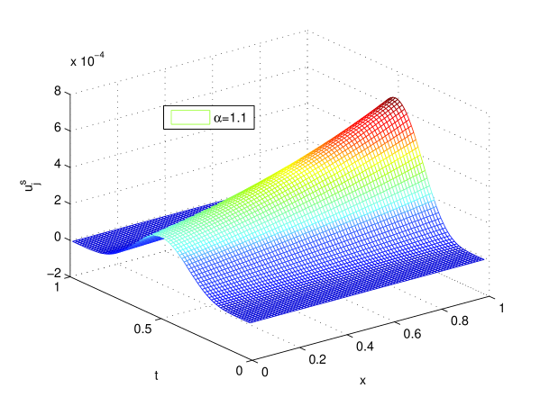
Figure 4.1: The numerical solution surface by difference scheme (20) with $\alpha=1.1$ and $\tau=h=\frac{1}{80}$.

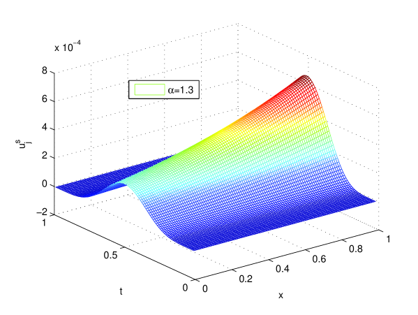
Figure 4.2: The numerical solution surface by difference scheme (20) with $\alpha=1.3$ and $\tau=h=\frac{1}{100}$.

5 Conclusions

In this work, we firstly derive even order fractional-compact numerical differential formulas for Riesz derivatives. Then a 4th-order numerical formula has been applied to solving the Riesz spatial fractional telegraph equation. Numerical results show that the experimental convergence orders are close to the theoretical convergence orders and confirm the efficiency of the new method developed in the current paper. These fractional-compact numerical differential formulas and the techniques can be also applied to $m$-dimensional $(m\geq 2)$ Riesz spatial differential equations.

Appendix I

Firstly, we list two lemmas as follows:

Lemma I. ([18]) The following inequalities hold:

$$\begin{array}[]{lll}\mathrm{(i)}\;\;1-x<\exp\left(-x\right)\;\;\textmd{for}\;\;0<x<1.\vspace{0.1 cm}\\ \displaystyle\mathrm{(ii)}\;\;1-x>\exp\left(-2x\right)\;\;\textmd{for}\;\;0<x\leq 0.7968.\end{array}$$

Lemma II. If functions $f(x)$ and $g(x)$ satisfy the conditions: $f(x)<0$ is an increasing function and $g(x)>0$ is a decreasing function, then $f(x)g(x)$ is an increasing function.

The proof is easy so is omitted here.

Now, we give the detailed proof for Theorem 1. Note that ${g}_{k}^{(\alpha)}={g}_{-k}^{(\alpha)}$, so we only consider the case $k\geq 0$.

Proof. (i) From the recursive relation

$$\begin{array}[]{rrr}\displaystyle{g}_{{}_{k}}^{(\alpha)}=\left(1-\frac{\alpha+1}{\frac{\alpha}{2}+k}\right){g}_{{}_{k-1}}^{(\alpha)},\end{array}$$

we easily obtain

$$\begin{array}[]{lll}\displaystyle\left|{g}_{{}_{k}}^{(\alpha)}\right|&<&\displaystyle\exp\left(-\frac{\alpha+1}{\frac{\alpha}{2}+k}\right)\left|{g}_{{}_{k-1}}^{(\alpha)}\right|<\exp\left(-\frac{\alpha+1}{\frac{\alpha}{2}+k}\right)\exp\left(-\frac{\alpha+1}{\frac{\alpha}{2}+k-1}\right)\left|{g}_{{}_{k-2}}^{(\alpha)}\right|\vspace{0.2 cm}\\ &<&\displaystyle\cdots<\exp\left(-\frac{\alpha+1}{\frac{\alpha}{2}+k}\right)\exp\left(-\frac{\alpha+1}{\frac{\alpha}{2}+k-1}\right)\ldots\exp\left(-\frac{\alpha+1}{\frac{\alpha}{2}+3}\right)\left|{g}_{{}_{2}}^{(\alpha)}\right|\vspace{0.2 cm}\\ &=&\displaystyle\exp\left(-(\alpha+1)\sum_{n=3}^{k}\frac{1}{\frac{\alpha}{2}+n}\right)\left|{g}_{{}_{2}}^{(\alpha)}\right|\end{array}$$

by using Lemma I.

Because function $\frac{1}{\frac{\alpha}{2}+x}$ is a decreasing function for $x>0$, then

$$\begin{array}[]{rrr}\displaystyle\sum_{n=3}^{k}\frac{1}{\frac{\alpha}{2}+n}>\int_{3}^{k+1}\frac{1}{\frac{\alpha}{2}+x}dx=\ln\frac{\frac{\alpha}{2}+k+1}{\frac{\alpha}{2}+3},\end{array}$$

so,

$$\begin{array}[]{rrr}\displaystyle\left|{g}_{{}_{k}}^{(\alpha)}\right|<\exp\left(-(\alpha+1)\ln\frac{\frac{\alpha}{2}+k+1}{\frac{\alpha}{2}+3}\right)\left|{g}_{{}_{2}}^{(\alpha)}\right|=-S(\alpha)\left(\frac{{\alpha}+6}{{\alpha}+2(k+1)}\right)^{\alpha+1},\;\;k\geq 3,\end{array}$$

where $S(\alpha)=\frac{\mathrm{\Gamma}(\alpha+1)}{\mathrm{\Gamma}\left(\frac{\alpha}{2}-1\right)\mathrm{\Gamma}\left(\frac{\alpha}{2}+3\right)}$.

Similarly, we also have the following estimation by equ. $(I1)$ and Lemma I,

$$\begin{array}[]{rrr}\displaystyle\left|{g}_{{}_{k}}^{(\alpha)}\right|>\exp\left(-\frac{2(\alpha+1)}{\frac{\alpha}{2}+k}\right)\left|{g}_{{}_{k-1}}^{(\alpha)}\right|>\exp\left(-2(\alpha+1)\sum_{n=3}^{k}\frac{1}{\frac{\alpha}{2}+n}\right)\left|{g}_{{}_{2}}^{(\alpha)}\right|.\end{array}$$

Notice

$$\begin{array}[]{rrr}\displaystyle\sum_{n=3}^{k}\frac{1}{\frac{\alpha}{2}+n}<\int_{2}^{k}\frac{1}{\frac{\alpha}{2}+x}dx=\ln\frac{\frac{\alpha}{2}+k}{\frac{\alpha}{2}+2},\end{array}$$

one has

$$\begin{array}[]{rrr}\displaystyle\left|{g}_{{}_{k}}^{(\alpha)}\right|>\exp\left(-2(\alpha+1)\ln\frac{\frac{\alpha}{2}+k}{\frac{\alpha}{2}+2}\right)\left|{g}_{{}_{2}}^{(\alpha)}\right|=-S(\alpha)\left(\frac{{\alpha}+4}{{\alpha}+2k}\right)^{2(\alpha+1)},\;\;k\geq 3.\end{array}$$

(ii) Since

$$\begin{array}[]{lll}\displaystyle\sum_{k=n}^{m}\frac{1}{(\alpha+2k)^{2(\alpha+1)}}&>&\displaystyle\int_{n}^{m+1}\frac{1}{(\alpha+2x)^{2(\alpha+1)}}dx\\ &=&\displaystyle\frac{1}{2(2\alpha+1)}\left[\left(\alpha+2n\right)^{-2\alpha-1}-\left(\alpha+2m+2\right)^{-2\alpha-1}\right],\end{array}$$

and

$$\begin{array}[]{lll}\displaystyle\sum_{k=n}^{m}\frac{1}{(\alpha+2k+2)^{\alpha+1}}&<&\displaystyle\int_{n-1}^{m}\frac{1}{(\alpha+2x+2)^{\alpha+1}}dx\\ &=&\displaystyle\frac{1}{2\alpha}\left[\left(\alpha+2n\right)^{-\alpha}-\left(\alpha+2m+2\right)^{-\alpha}\right],\end{array}$$

one gets,

$$\begin{array}[]{lll}\displaystyle\sum_{k=n}^{m}\left|g_{{}_{k}}^{(\alpha)}\right|&>&\displaystyle-S(\alpha)\left(\alpha+4\right)^{2(\alpha+1)}\sum_{k=n}^{m}\frac{1}{(\alpha+2k)^{2(\alpha+1)}}\vspace{0.2 cm}\\ &>&\displaystyle\displaystyle\frac{\left(\alpha+4\right)^{2(\alpha+1)}}{2(2\alpha+1)}P_{1}(m,n,\alpha),\end{array}$$

where $P_{1}(m,n,\alpha)=-S(\alpha)\left[\left(\alpha+2n\right)^{-2\alpha-1}-\left(\alpha+2m+2\right)^{-2\alpha-1}\right]$, $n\geq 3$, and

$$\begin{array}[]{lll}\displaystyle\sum_{k=n}^{m}\left|g_{k}^{(\alpha)}\right|&<&\displaystyle-S(\alpha)\left(\alpha+6\right)^{\alpha+1}\sum_{k=n}^{m}\frac{1}{(\alpha+2(k+1))^{\alpha+1}}\\ \vspace{0.2 cm}&<&\displaystyle\displaystyle\frac{\left(\alpha+6\right)^{\alpha+1}}{2\alpha}P_{2}(m,n,\alpha),\end{array}$$

where $P_{2}(m,n,\alpha)=-S(\alpha)\left[\left(\alpha+2n\right)^{-\alpha}-\left(\alpha+2m+2\right)^{-\alpha}\right]$, $n\geq 3$.

(iii) Just letting $m=\infty$ in $(I2)$ and $(I3)$ gives the proof.

(iv) By using the following formula [12]

$$\begin{array}[]{lll}\displaystyle\int_{0}^{\frac{\pi}{2}}\left(\cos x\right)^{\alpha}\cos\left(\beta x\right)\mathrm{d}x=\frac{\pi}{2^{1+\alpha}}\frac{\mathrm{\Gamma}(1+\alpha)}{\mathrm{\Gamma}\left(1+\frac{\alpha+\beta}{2}\right)\mathrm{\Gamma}\left(1+\frac{\alpha-\beta}{2}\right)},\;\;\;\mathrm{Re}(\alpha)>-1,\end{array}$$

one can gets

$$\begin{array}[]{lll}\displaystyle g_{{}_{0}}^{(\alpha)}=\frac{\mathrm{\Gamma}(1+\alpha)}{\mathrm{\Gamma}\left(1+\frac{\alpha}{2}\right)\mathrm{\Gamma}\left(1+\frac{\alpha}{2}\right)}=\frac{2^{1+\alpha}}{\pi}\int_{0}^{\frac{\pi}{2}}\left(\cos x\right)^{\alpha}\mathrm{d}x\leq\frac{2^{1+\alpha}}{\pi}\int_{0}^{\frac{\pi}{2}}\cos x\mathrm{d}x=\frac{2^{1+\alpha}}{\pi}\end{array}$$

for $1<\alpha<2$.

In addition, $g_{{}_{0}}^{(\alpha)}$ is usually represented by using the beta function $B(\cdot,\cdot)$, i.e.,

$$\begin{array}[]{lll}\displaystyle g_{{}_{0}}^{(\alpha)}=\frac{\mathrm{\Gamma}(1+\alpha)}{\mathrm{\Gamma}\left(1+\frac{\alpha}{2}\right)\mathrm{\Gamma}\left(1+\frac{\alpha}{2}\right)}=\frac{\mathrm{\Gamma}(2+\alpha)}{(1+\alpha)\mathrm{\Gamma}\left(1+\frac{\alpha}{2}\right)\mathrm{\Gamma}\left(1+\frac{\alpha}{2}\right)}=\frac{1}{(1+\alpha)B\left(\frac{2+\alpha}{2},\frac{2+\alpha}{2}\right)},\end{array}$$

and in which

$$\begin{array}[]{lll}\displaystyle B\left(\frac{\alpha}{2},\frac{\alpha}{2}\right)=2\int_{0}^{\frac{\pi}{2}}\left(\sin x\right)^{\alpha-1}\left(\cos x\right)^{\alpha-1}\mathrm{d}x=\frac{1}{2^{\alpha-2}}\int_{0}^{\frac{\pi}{2}}\left(\sin 2x\right)^{\alpha-1}\mathrm{d}x\leq\frac{\pi}{2^{\alpha-1}},\end{array}$$

so, we have

$$\begin{array}[]{lll}\displaystyle g_{{}_{0}}^{(\alpha)}\geq\frac{2^{1+\alpha}}{\pi(1+\alpha)}.\end{array}$$

From [33] we known that

$$\begin{array}[]{lll}\displaystyle\sum\limits_{k=-\infty,k\neq 0}^{\infty}\left|\right.{g}_{{}_{k}}^{(\alpha)}\left|\right.={g}_{{}_{0}}^{(\alpha)},\end{array}$$

that is,

$$\begin{array}[]{lll}\displaystyle\frac{2^{1+\alpha}}{(1+\alpha)\pi}\leq\sum\limits_{k=-\infty,k\neq 0}^{\infty}\left|\right.{g}_{{}_{k}}^{(\alpha)}\left|\right.\leq\frac{2^{1+\alpha}}{\pi}.\end{array}$$

(v) When $k=0$, then $g_{{}_{0}}^{(\alpha)}=\frac{\mathrm{\Gamma}(\alpha+1)}{\mathrm{\Gamma}^{2}\left(\frac{\alpha}{2}+1\right)}$, and $\ln g_{{}_{0}}^{(\alpha)}=\ln\mathrm{\Gamma}(\alpha+1)-2\ln\mathrm{\Gamma}\left(\frac{\alpha}{2}+1\right)$.

$$\begin{array}[]{lll}\displaystyle\frac{g_{0}^{(\alpha)^{{}^{\prime}}}}{g_{0}^{(\alpha)}}&=&\displaystyle\psi(\alpha+1)-\psi\left(\frac{\alpha}{2}+1\right)\vspace{0.2 cm}\\ &=&\displaystyle\int_{0}^{\infty}\frac{\exp(-t)-\exp(-(\alpha+1)t)}{1-\exp(-t)}\mathrm{d}t-\int_{0}^{\infty}\frac{\exp(-t)-\exp\left(-\left(\frac{\alpha}{2}+1\right)t\right)}{1-\exp\left(-t\right)}\mathrm{d}t\vspace{0.2 cm}\\ &=&\displaystyle\int_{0}^{\infty}\frac{\exp(-(\alpha+1)t)\left[\exp\left(\frac{\alpha}{2}t\right)-1\right]}{1-\exp(-t)}\mathrm{d}t\vspace{0.2 cm}\\ &=&\displaystyle\int_{0}^{\infty}\frac{\exp(-(\alpha+1)t)}{1-\exp(-t)}\left(\sum_{n=0}^{\infty}\frac{\left(\frac{\alpha}{2}\right)^{n}}{n!}t^{n}\right)\mathrm{d}t>0,\end{array}$$

where $g_{0}^{(\alpha)^{{}^{\prime}}}=\frac{\mathrm{d}g_{0}^{(\alpha)}}{\mathrm{d}\alpha}$. Since $g_{0}^{(\alpha)}>0$, $g_{0}^{(\alpha)^{{}^{\prime}}}>0$, that is, $g_{0}^{(\alpha)}$ is an increasing function with respect to $\alpha\in(1,2)$.

When $k=1$, $g_{1}^{(\alpha)}=-\frac{\mathrm{\Gamma}(\alpha+1)}{\mathrm{\Gamma}\left(\frac{\alpha}{2}\right)\mathrm{\Gamma}\left(\frac{\alpha}{2}+2\right)}$, similarly to case $k=0$, we have

$$\begin{array}[]{lll}\displaystyle\frac{\mathrm{d}}{\mathrm{d}\alpha}\ln\left(-g_{1}^{(\alpha)}\right)&=&\displaystyle\frac{g_{1}^{(\alpha)^{{}^{\prime}}}}{g_{1}^{(\alpha)}}=\psi(\alpha+1)-\frac{1}{2}\psi\left(\frac{\alpha}{2}\right)-\frac{1}{2}\psi\left(\frac{\alpha}{2}+2\right)\vspace{0.2 cm}\\ &=&\displaystyle\int_{0}^{\infty}\frac{\frac{1}{2}\exp\left(\frac{-\alpha}{2}t\right)+\frac{1}{2}\exp\left(-\left(\frac{\alpha}{2}+2\right)t\right)-\exp(-(\alpha+1)t)}{1-\exp(-t)}\mathrm{d}t\vspace{0.2 cm}\\ &\geq&\displaystyle\int_{0}^{\infty}\frac{\exp\left(-\left(\frac{\alpha}{2}+1\right)t\right)-\exp(-(\alpha+1)t)}{1-\exp(-t)}\mathrm{d}t>0.\end{array}$$

Because of $g_{1}^{(\alpha)}<0$, then $g_{1}^{(\alpha)^{{}^{\prime}}}<0$, i.e, $g_{1}^{(\alpha)}$ is a decreasing function.

When $k=2$,

$$\begin{array}[]{lll}\displaystyle g_{2}^{(\alpha)}=\frac{\mathrm{\Gamma}(\alpha+1)}{\mathrm{\Gamma}\left(\frac{\alpha}{2}+3\right)\mathrm{\Gamma}\left(\frac{\alpha}{2}-1\right)}=-\frac{2\left(1-\frac{\alpha}{2}\right)\mathrm{\Gamma}(\alpha)}{\left(1+\frac{\alpha}{2}\right)\left(2+\frac{\alpha}{2}\right)\mathrm{\Gamma}^{2}\left(\frac{\alpha}{2}\right)}.\end{array}$$

According to another definition of $\mathrm{\Gamma}(\alpha)$ [32]:

$$\begin{array}[]{lll}\displaystyle\mathrm{\Gamma}(\alpha)=\frac{1}{\alpha}\prod\limits_{n=1}^{\infty}\frac{\left(1+\frac{1}{n}\right)^{\alpha}}{1+\frac{\alpha}{n}},\end{array}$$

it is easily known that

$$\begin{array}[]{lll}\displaystyle\frac{\mathrm{\Gamma}(\alpha)}{\mathrm{\Gamma}^{2}\left(\frac{\alpha}{2}\right)}=\frac{\alpha}{4}\prod\limits_{n=1}^{\infty}\frac{\left(1+\frac{\alpha}{2n}\right)^{2}}{1+\frac{\alpha}{n}}.\end{array}$$

Substituting the above equation into $g_{2}^{(\alpha)}$ yields

$$\begin{array}[]{lll}\displaystyle g_{2}^{(\alpha)}=-\frac{\alpha(2-\alpha)}{(2+\alpha)(4+\alpha)}\prod\limits_{n=1}^{\infty}\frac{\left(1+\frac{\alpha}{2n}\right)^{2}}{1+\frac{\alpha}{n}}.\end{array}$$

$$\begin{array}[]{lll}\displaystyle\frac{g_{2}^{(\alpha)^{{}^{\prime}}}}{g_{2}^{(\alpha)}}=\frac{\mathrm{d}}{\mathrm{d}\alpha}\ln\left(-g_{2}^{(\alpha)}\right)=\frac{1}{2}\sum_{n=1}^{\infty}\frac{\alpha}{\left(n+\frac{\alpha}{2}\right)(n+\alpha)}-\left(\frac{1}{2-\alpha}-\frac{1}{\alpha}+\frac{1}{2+\alpha}+\frac{1}{4+\alpha}\right).\end{array}$$

Let

$$\begin{array}[]{lll}\displaystyle S(\alpha)=\frac{1}{2}\sum_{n=1}^{\infty}\frac{1}{\left(n+\frac{\alpha}{2}\right)(n+\alpha)},\end{array}$$

and

$$\begin{array}[]{lll}\displaystyle f_{1}(\alpha)=\frac{1}{\alpha}\left(\frac{1}{2-\alpha}-\frac{1}{\alpha}+\frac{1}{2+\alpha}+\frac{1}{4+\alpha}\right).\end{array}$$

Then

$$\begin{array}[]{lll}\displaystyle S(\alpha)<\sum_{n=1}^{\infty}\frac{2}{(2n+1)^{2}}=\sum_{n=1}^{\infty}\frac{2}{(2n-1)^{2}}-2=\frac{\pi^{2}}{4}-2,\end{array}$$

and

$$\begin{array}[]{lll}\displaystyle f_{1}^{{}^{\prime}}(\alpha)=\frac{8\left[3\alpha^{5}+10\alpha^{3}+12+8(2-\alpha)+4(2\alpha-3)^{2}\right]}{\alpha^{3}(2-\alpha)^{2}(2+\alpha)^{2}(4+\alpha)^{2}}>0,\end{array}$$

that is to say $f_{1}(\alpha)$ is an increasing function and its minimum value is $f_{1}(\alpha)_{\min}=f_{1}(1)=\frac{8}{15}.$

So,

$$\begin{array}[]{lll}\displaystyle\frac{g_{2}^{(\alpha)^{{}^{\prime}}}}{g_{2}^{(\alpha)}}=\alpha(S(\alpha)-f_{1}(\alpha))<\alpha\left(\frac{\pi^{2}}{4}-2-\frac{8}{15}\right)<\alpha\left(\frac{3.15^{2}}{4}-2-\frac{8}{15}\right)=-\frac{253}{4800}\alpha.\end{array}$$

Since $g_{2}^{(\alpha)}<0$, it follows that $g_{2}^{(\alpha)^{{}^{\prime}}}>0$, i.e., $g_{2}^{(\alpha)}$ is an increasing function with respect to $\alpha\in(1,2)$.

When $k=3$,

$$\begin{array}[]{lll}\displaystyle g_{3}^{(\alpha)}=-\frac{2\left(1-\frac{\alpha}{2}\right)\left(2-\frac{\alpha}{2}\right)\mathrm{\Gamma}(\alpha)}{\left(1+\frac{\alpha}{2}\right)\left(2+\frac{\alpha}{2}\right)\left(3+\frac{\alpha}{2}\right)\mathrm{\Gamma}^{2}\left(\frac{\alpha}{2}\right)}=-\frac{\alpha(2-\alpha)(4-\alpha)}{(2+\alpha)(4+\alpha)(6+\alpha)}\prod\limits_{n=1}^{\infty}\frac{\left(1+\frac{\alpha}{2n}\right)^{2}}{1+\frac{\alpha}{n}}.\end{array}$$

$$\begin{array}[]{lll}\displaystyle\frac{g_{3}^{(\alpha)^{{}^{\prime}}}}{g_{3}^{(\alpha)}}=\alpha(S(\alpha)-f_{2}(\alpha)),\end{array}$$

where $\displaystyle f_{2}(\alpha)=\frac{1}{\alpha}\left(\frac{1}{2-\alpha}+\frac{1}{4-\alpha}-\frac{1}{\alpha}+\frac{1}{2+\alpha}+\frac{1}{4+\alpha}+\frac{1}{6+\alpha}\right)>0.$

So,

$$\begin{array}[]{lll}\displaystyle\frac{g_{3}^{(\alpha)^{{}^{\prime}}}}{g_{3}^{(\alpha)}}=\alpha(S(\alpha)-f_{2}(\alpha))<\alpha\left(\frac{\pi^{2}}{4}-2-\frac{106}{105}\right)<\alpha\left(\frac{3.15^{2}}{4}-2-\frac{106}{105}\right)=-\frac{485}{917}\alpha.\end{array}$$

It immediately follows that $g_{3}^{(\alpha)}$ is an increasing function.

Finally, we consider the cases $k\geq 4$. From [26] one has

$$\begin{array}[]{lll}\displaystyle g_{k}^{(\alpha)}=\frac{(-1)^{k}\mathrm{\Gamma}(\alpha+1)}{\mathrm{\Gamma}\left(\frac{\alpha}{2}-k+1\right)\mathrm{\Gamma}\left(\frac{\alpha}{2}+k+1\right)}=-\frac{\sin\left(\frac{\pi}{2}\alpha\right)}{\pi}\frac{\mathrm{\Gamma}(\alpha+1)\mathrm{\Gamma}\left(k-\frac{\alpha}{2}\right)}{\mathrm{\Gamma}\left(\frac{\alpha}{2}+k+1\right)}.\end{array}$$

Letting

$$\begin{array}[]{lll}\displaystyle z(\alpha)=-\frac{\sin\left(\frac{\pi}{2}\alpha\right)}{\pi},\;\;z_{{}_{k}}(\alpha)=\frac{\mathrm{\Gamma}(\alpha+1)\mathrm{\Gamma}\left(k-\frac{\alpha}{2}\right)}{\mathrm{\Gamma}\left(\frac{\alpha}{2}+k+1\right)},\end{array}$$

obviously, $z(\alpha)<0$ is an increasing function with respect to $\alpha$ for $1<\alpha<2$. Meanwhile, we have

$$\begin{array}[]{lll}\displaystyle\ln z_{{}_{k}}(\alpha)=\ln\mathrm{\Gamma}(\alpha+1)+\ln\mathrm{\Gamma}\left(k-\frac{\alpha}{2}\right)-\ln\mathrm{\Gamma}\left(\frac{\alpha}{2}+k+1\right).\end{array}$$

Furthermore, it follows that

$$\begin{array}[]{lll}\displaystyle\frac{z_{{}_{k}}(\alpha)^{{}^{\prime}}}{z_{{}_{k}}(\alpha)}&=&\displaystyle\psi(\alpha+1)-\frac{1}{2}\psi\left(k-\frac{\alpha}{2}\right)-\frac{1}{2}\psi\left(\frac{\alpha}{2}+k+1\right)\vspace{0.2 cm}\\ &=&\displaystyle\int_{0}^{\infty}\frac{\frac{1}{2}\exp\left(-\left(k-\frac{\alpha}{2}\right)t\right)+\frac{1}{2}\exp\left(-\left(\frac{\alpha}{2}+k+1\right)t\right)-\exp(-(\alpha+1)t)}{1-\exp(-t)}\mathrm{d}t\vspace{0.2 cm}\\ &=&\displaystyle\int_{0}^{\infty}\frac{\exp\left(-\left(\frac{\alpha}{2}+k+1\right)t\right)\left[\frac{1}{2}\exp((\alpha+1)t)+\frac{1}{2}-\exp((k-\frac{\alpha}{2})t)\right]}{1-\exp(-t)}\mathrm{d}t\vspace{0.2 cm}\\ &=&\displaystyle\int_{0}^{\infty}\frac{\exp\left(-\left(\frac{\alpha}{2}+k+1\right)t\right)}{1-\exp(-t)}\left(\sum_{n=1}^{\infty}\frac{\frac{1}{2}(\alpha+1)^{n}-\left(k-\frac{\alpha}{2}\right)^{n}}{n!}t^{n}\right)\mathrm{d}t.\end{array}$$

If $k\geq 4$, then $\frac{1}{2}(\alpha+1)^{n}-\left(k-\frac{\alpha}{2}\right)^{n}<0$ for $1<\alpha<2$. At this moment, we have $z_{{}_{k}}(\alpha)^{{}^{\prime}}<0$, i.e., $z_{{}_{k}}(\alpha)$ is a decreasing function. So $g_{k}^{(\alpha)}=z(\alpha)z_{{}_{k}}(\alpha)$ is an increasing function for $k\geq 4$ by using Lemma II.

Therefore, all this finishes the proof of Theorem 1. $\blacksquare$

References

[1] Agrawal. O. P.: Solution for a fractional diffusion-wave equation defined in a bounded domain.
Nonlinear Dyn., 29, 145–155 (2002).
[2] Al-Saqabi. B., Boyadjiev. L., Luchko. Y.:
Comments on employing the Riesz-Feller
derivative in the Schrödinger equation, Eur. Phys. J. Special Topics, 222, 1779–1794 (2013).
[3] Buldyrev. S. V., Havlin. S., Kazakov. A. Ya., da Luz. M. G. E., Raposo. E. P.,
Stanley. H. E., Viswanathan. G. M.:
Average time spent by Lévy flights and walks on an interval with absorbing boundarie,
Phys. Rev. E., 64, 041108, (2001).
[4] Bhrawy. A. H., Zaky. M. A., Machado. J. A. T.: Numerical solution of the two-sided space-time
fractional telegraph equation via Chebyshev Tau
approximation, Nonlinear Dyn., 81, 1023–1052 (2015).
[5]
Cao. J., Xu. C.: A high order scheme for the numerical solution of the fractional ordinary differential
equations, J. Comput. Phys., 238, 154–168 (2013).
[6] Çelik. C., Duman. M.: Crank-Nicolson method for the fractional
diffusion equation with the Riesz fractional derivative, J. Comput.
Phys., 231, 1743-1750 (2012).
[7] Chen. S., Jiang. X., Liu. F., Turner. I.,
High order unconditionally stable difference schemes for the
Riesz space-fractional telegraph equation, J. Comput. Appl. Math.,
278, 119–129 (2015).
[8]Diethelm, K.: The analysis of fractional differential equations. Springer, Berlin, 2010.
[9]Diethelm, K.: Smoothness properties of solutions of Caputo-type
fractional differential equations, Fract. Calc. Appl. Anal., 10(2), 151–160 (2007).
[10] Ding. H. F., Li. C. P., Chen. Y. Q.: High-order Algorithms
for Riesz Derivative and Their Applications (I), Abstract and Applied
Analysis 2014, Article ID 653797 (17 pages), 2014.
[11]
Ding. H. F., Li. C. P., Chen. Y. Q.: High-order
algorithms for Riesz derivative and their applications
(II), J. Comput. Phys., 293, 218–237 (2015).
[12]
Erdélyi. A., Magnus. W., Oberhettinger. F., Tricomi. F. G., Higher
Transcendental Functions, Vol. 1, McGraw-Hill, New York, 1953.
[13] Horn. R. A., Johnson. C. R.:, Matrix Analysis, Cambridge University Press, 1986.
[14]
Hao. Z., Sun. Z., Cao. W.: A fourth-order approximation of fractional derivatives with its applications,
J. Comput. Phys., 281, 787–805 (2015).
[15]
Gao. G. H., Sun. Z. Z., Zhang. H. W.: A new fractional numerical differentiation
formula to approximate the Caputo fractional derivative and its applications,
J. Comput. Phys., 259, 33–50 (2014).
[16] Janaswamy. R., On random time and on the relation between wave
and telegraph, IEEE Trans. Antennas and Propagation, 61, 2735–2744 (2013).
[17]
Kershaw. D.: Some extensions of W. Gautschi s inequalities for the gamma
function, Math. Comp., 41, 607–611 (1983).
[18] Kuang. J. C.: Applied Inequalities, 2nd ed.,
Shandong Scienic and Technology Press, Jinan, 2012.
[19] Langlands. T. A. M., Henry. B. I.: The accuracy and
stability of an implicit solution method for the fractional
diffusion equation, J. Comput. Phys., 205, 719–736 (2005).
[20]
Li. C. P., Chen. A., Ye. J. J.: Numerical approaches to fractional calculus and fractional
ordinary differential equation, J. Comput. Phys., 230, 3352–3368 (2011).
[21] Lin. C. Y., Gu. M. H., Young. D. L.: The time-marching method of fundemental solutions
for multi-dimensional telegraph euqtions, CMC Comput. Mater.
Continua, 18, 43–68 (2010).
[22]
Li. C. P., Wu. R. F., Ding. H. F.: High-order approximation to Caputo derivatives and Caputo-type advection diffusion equation (I),
Commun.
Appl. Ind. Math., 2015, DOI: 10.1685/journal.caim.536.
[23] Li, C. P., Zeng, F. H.: Numerical Methods for Fractional Calculus, Chapman and Hall/CRC, New York, 2015.
[24]
Meerschaert. M. M., Scheffler. H. P., Tadjeran. C.: Finite
difference methods for two–dimensional fractional dispersion
equation, J. Comput. Phys., 211, 249–261 (2006).
[25]Metzler. R., Klafter. J.: The random walk s guide to anomalous diffusion: A fractional dynamics
approach, Phys. Rep., 339, 1-77 (2000).
[26]
Ortigueira. M. D.: Riesz potential operators and inverses via
fractional centred derivatives, Int. J. Math. Math. Sci., 48391,
1–12 (2006).
[27] Orsingher. E., Beghin. L.: Time-fractional telegraph equation and telegraph processes with Brownian time,
Probab. Theory Related Fields, 128, 141–160 (2004).
[28]
Oldham. K. B., Spanier. J.: The Fractional Calculus, Dover Publications, Mineola, New work, renewed, 2002.
[29] Orsingher. E., Zhao. X.: The space-fractional telegraph equation and the related fractional telegraph process,
Chin. Ann. Math., 24B, 1–12 (2003).
[31]Quarteroni. A., Sacco. R., Saleri. F.: Numerical
Mathematics, Springer, New York, 2007.
[32]
Samko. S. G., Kilbas. A. A., Marichev. O. I.: Fractional Integrals and Derivatives: Theory and Applications,
Gordon and Breach, New York, 1993.
[33]Shen. S., Liu. F., Anh. V., Turner. I., Chen. J.,:
A novel numerical approximation for the space fractional
advection-dispersion equation, IMA J. Appl. Math., 79, 431–444 (2014).
[34]
Tuan. V. K., Gorenflo R.: Extrapolation to the limit for numerical fractional differentiation,
Z. Angew. Math. Mech., 75, 646–648 (1995).
[35]
Tian. Z. F., Liang. X., Yu. P. X.:
A higher order compact finite difference algorithm for solving the incompressible Navier-Stokes equations,
Int. J. Numer. Meth. Eng., 6, 511–532 (2011).
[36]
Tian. W. Y., Zhou. H., Deng. W. H.: A class of second order difference approximations for solving space
fractional diffusion equations, Math. Comput., 84, 1703–1727 (2015).
[37]
Wang. Z., Vong. S.: Compact difference schemes for the modified anomalous fractional subdiffusion
equation and the fractional diffusion-wave equation, J. Comput. Phys., 277, 1–15 (2014).
[38]Wang. H., Basu. T.: A fast finite difference method for two-dimensional space-fractional diffusion equations,
SIAM J. Sci. Comput., 34, A2444–A2458 (2012).
[39] Wang. H., Du N.: A super fast-preconditioned iterative method for steady-state space-fractional diffusion
equations, J. Comput. Phys., 240, 49–57 (2013).
[40]Zhang. W. S.: Finite difference methods for partial
differential equations in science computation, Higher
Education Press, Beijing, 2006.
[41] Zhou. H., Tian. W. Y., Deng. W. H.: Quasi-compact finite
difference schemes for space fractional diffusion equations, J. Sci.
Comput., 56, 45–66 (2013).