Crossover from rotational to stochastic sandpile universality in the random rotational sandpile model

Abstract

In the rotational sandpile model, either the clockwise or the anti-clockwise toppling rule is assigned to all the lattice sites. It has all the features of a stochastic sandpile model but belongs to a different universality class than the Manna class. A crossover from rotational to Manna universality class is studied by constructing a random rotational sandpile model and assigning randomly clockwise and anti-clockwise rotational toppling rules to the lattice sites. The steady state and the respective critical behaviour of the present model are found to have a strong and continuous dependence on the fraction of the lattice sites having the anti-clockwise (or clockwise) rotational toppling rule. As the anti-clockwise and clockwise toppling rules exist in equal proportions, it is found that the model reproduces critical behaviour of the Manna model. It is then further evidence of the existence of the Manna class, in contradiction with some recent observations of the non-existence of the Manna class.

I Introduction

A sandpile is a prototypical model to study self-organized criticality (SOC) Bak (1996); *jensen; *pruessner, which refers to the intrinsic tendency of a wide class of slowly driven systems to evolve spontaneously to a non equilibrium steady state characterized by long-range spatiotemporal correlation and power-law scaling behaviour. Several crossover phenomena from one sandpile universality class to the other are reported in the literature on sandpile models. For example, a crossover from Bak, Tang and Wiesenfeld (BTW) Bak et al. (1987) to the stochastic Zhang model was observed by O. Biham et al. Biham et al. (2001) by controlling the fraction of energy distributed to the nearest neighbours in a toppling. A crossover from the deterministic Zhang model Zhang (1989) to the stochastic sandpile model (SSM) Manna (1991a, b); Dhar (1999a) was studied by Lübeck Lübeck (2000a) by controlling the threshold condition. A crossover from the directed sandpile model (DSM) Dhar and Ramaswamy (1989) to the directed percolation (DP) class Marro and Dickman (1999); *henkel; *DPhinrichsenAIP00 was observed by Tadić and Dhar by introducing a stickiness parameter in the DSM Tadić and Dhar (1997). The crossover phenomena studied in these models are usually from a deterministic to a stochastic model. However, the universality class of a sandpile model is believed to be determined by the underlying symmetry present in the model Rossi et al. (2000). A crossover from one sandpile universality class to another then requires a change in the underlying symmetry of a given model. It is therefore intriguing to study a crossover phenomenon within the stochastic class of models with different symmetries in the toppling rule, and to look for spontaneous symmetry breaking in the system as one of the system parameters is tuned. Two such stochastic sandpile models are the SSM Dhar (1999a) and the rotational sandpile model (RSM) Santra et al. (2007); Ahmed and Santra (2012a). The SSM is governed by externally imposed stochastic toppling rules. On the other hand, the RSM is governed by deterministic rotational toppling rules (except the very first toppling) and has broken mirror symmetry. Such a model can be useful in studying the avalanche dynamics of charged particles in the presence of a uniform magnetic field. In the RSM, an internal stochasticity appears due to a superposition of toppling waves from different directions during time evolution. Eventually, that induces all the features of a stochastic sandpile model, such as toppling imbalance, negative time auto correlation, and existence of finite-size scaling (FSS) into the RSM Santra et al. (2007); Ahmed and Santra (2010a, 2011, 2012a). The RSM is thus a stochastic model, but it belongs to a completely different universality class than the Manna class of the SSM. The question is whether it would be possible to reproduce the critical behaviour of the SSM of Manna type in a model such as the RSM, which is stochastic due to its internal dynamics. Moreover, there is a long standing debate in the study of SOC as absorbing state phase transitions (APT) Dickman et al. (1998); Muñoz et al. (1999); Vespignani et al. (2000) stating that the stochastic universality class or the Manna class is essentially the DP universality class. There is continuing evidences in favour Bonachela et al. (2006); *bonachelaPHYA07; *bonachelaPRE08; *leePRL13; *leePRE13; *leePRE14a; *leePRE14b and against Mohanty and Dhar (2002); *mohantyPHYA07; *basuPRL12 the existence of the so-called Manna class. If due to any external condition on the RSM, it reproduces the critical behaviour of the Manna model, that will be additional independent evidence for the existence of the Manna class.

In this paper, the crossover from one stochastic universality class to another is studied by constructing a random rotational sandpile model (RRSM) and the existence of the Manna class is discussed in the context of random mixing of two conflicting rotational toppling rules in the model.

II The model

The RRSM is defined on a two-dimensional ($2D$) square lattice of size $L\times L$. Initially, all lattice sites are assigned with the clockwise toppling rule (CTR). A fraction $p$ of lattice sites are then changed to the anti-clockwise toppling rule (ATR) randomly. The toppling rules assigned to the lattice sites remain unchanged during the time evolution of the system and hence this can be considered as a quenched random configuration of the toppling rules. The RSM Santra et al. (2007) was defined for the presence of only one type of toppling rule either CTR or ATR. Since the sandpile dynamics is independent of the sense of rotations, the RSMs with either CTR or ATR have the same critical behaviour.

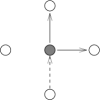
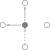
(a) CTR (b) ATR

Figure 1: The two toppling rules of RRSM, CTR, and ATR are demonstrated on a square lattice in (a) and (b), respectively. The active site in grey is at the center and it has received the last sand grain from the bottom (say), represented by a dashed arrow. The directions of sand flow from the active site are represented by solid arrows. In (a), due to CTR, one sand grain goes to the right and the other goes up, whereas in (b), due to ATR, one sand grain goes to the left and the other goes up.

Each lattice site $i$, irrespective of the type of toppling rule it has, is assigned with a positive integer $h_{i}$ representing the height (the number of sand grains) of the sand column. Initially, all $h_{i}$s are set to zero. The system is driven by adding sand grains, one at a time, to randomly chosen lattice sites $i$. The critical height of the model is taken as $h_{c}=2$. As the height of a sand column $h_{i}$ becomes equal to or greater than the critical height $h_{c}$, i.e., $h_{i}\geq h_{c}$, the site becomes active and bursts into a toppling activity. On the very first toppling of an active site, two sand grains are given away to two randomly selected nearest neighbours out of the four nearest neighbours on a square lattice. As soon as a site $j$ receives a sand grain, the direction $d_{j}$ from which the grain was received is assigned to it besides incrementing the height of the sand column $h_{j}$ by one unit. The value of $d_{j}$ can change from $1$ to $4$, as there are four possible directions on a square lattice. The directions from an active site $i$ are defined as $d_{i}=1$ for left, $d_{i}=2$ for up, $d_{i}=3$ for right and $d_{i}=4$ for down. As the avalanche propagates, the direction $d_{i}$ and height $h_{i}$ are updated upon receiving a sand grain, and only the information regarding the direction from which the last sand grain was received is kept. The next active sites with $h_{i}\geq h_{c}$ in the avalanche will topple following a deterministic rotational toppling rule. The toppling rules for an active site $i$ that has received the last sand grain from a direction $d_{i}$ are given below. If the active site $i$ is with CTR, the sand distribution is given by

$${\rm CTR:}\ \ h_{i}\rightarrow h_{i}-2,\ \ h_{j}\rightarrow h_{j}+1,\ \ \ j=d_{i},d_{i+1},$$ (1)

where one sand grain goes along $d_{i}$ and the other goes in a clockwise direction with respect to $d_{i}$. If the active site $i$ is with ATR, the sand distribution is given by

$${\rm ATR:}\ \ h_{i}\rightarrow h_{i}-2,\ \ h_{j}\rightarrow h_{j}+1,\ \ \ j=d_{i},d_{i-1},$$ (2)

where one sand grain goes along $d_{i}$ and the other goes in an anti-clockwise direction with respect to $d_{i}$. If the index $j$ becomes $5$, it is taken to be $1$; if it becomes $0$, it is taken to be $4$. The CTR and ATR are demonstrated in Fig. 1 on a square lattice. The avalanche stops if there is no active site present and the system becomes under critical. The next sand grain is then added. As RSM, the RRSM is non-Abelian Dhar (1999b); *dharPHYA06 and it has no toppling balance Karmakar et al. (2005).

In the following, the results of the RRSM are compared with those of the original RSM Santra et al. (2007) and the SSM Dhar (1999a). The SSM considered here is a modified version of the Manna model Manna (1991a, b) known as the Dhar Abelian model. The toppling rule in this SSM is that two sand grains of an active site are given to two randomly selected nearest-neighbour sites out of four possible nearest neighbours on a square lattice and the height of the active site is reduced by $2$. The remaining sand grains remain at the present site.

Figure 2: Plot of ${\bar{h}}_{p}(n)$ against $n$, the number of sand grains added, for $p=0.0,0.1,0.25$ and $0.5$ for RRSM on $L=2048$. In the inset, the average steady state height $\langle h(p)\rangle$ is plotted against $p$. The dashed line represents the average steady state height of the SSM studied on $L=2048$.

III Steady state

The steady state of a sandpile model corresponds to constant currents of sand influx and outflux. Consequently, the average height of the sand columns remains constant over time. For a given value of $p$ in the RRSM, the mean height ${\bar{h}}_{p}(n)$ of the sand columns is expected to be constant over the number of sand grains $n$ added (equivalent to time) to the system. It can be defined as

$${\bar{h}}_{p}(n)=\frac{1}{L^{2}}\sum_{i=1}^{L^{2}}h_{i}(p,n)$$ (3)

for a system size $L$. For different values of $p$, ${\bar{h}}_{p}(n)$ for $L=2048$ is plotted against $n$, the number of sand grains added in Fig. 2. After the addition of a sufficiently large number of sand grains, the system reaches a steady state corresponding to a given value of $p$. In order to study the effect of $p$ on the steady state height, the saturated average height $\langle h(p)\rangle$ of the sand columns in the steady state for a given value of $p$ is estimated taking the average over the last $10^{5}$ sand grains on every $64$ random configurations of toppling rules. Note that, no configurational average is required for $p=0$ and $1$. In the inset of Fig. 2, $\langle h(p)\rangle$ is plotted against $p$ for $L=2048$. It can be seen that the saturated average height of the sand columns at the steady state decreases as $p$ is varied from $0$ (or $1$) to $0.5$, and it attains a minimum value at $p=0.5$. The values of $\langle h(p)\rangle$ are found to be symmetric about $p=0.5$, as expected. The average heights at $p=0$ and $1$ are found to be that of the RSM Santra et al. (2007), whereas at $p=0.5$ the average height is that of the SSM. The time-averaged steady state-height for the SSM for $L=2048$ is measured independently, and it is found to be $0.7162\pm 0.0001$. It is represented by a dashed line in the inset of Fig. 2. It can be noted here that the measured value of the average sand column height for the SSM is in good agreement with that of the driven dissipative sandpile in the context of the precursor to a catastrophe study Pradhan and Chakrabarti (2001) as well as the critical point of the APT of a fixed energy sandpile model Vespignani et al. (2000). Thus, the steady-state heights corresponding to different values of $p$ are not only different from each other but also very different from that of the SSM.

IV Results and discussion

The critical properties of RRSM are characterized studying the properties associated with avalanches in the steady states at different values of $p$ and the system size $L$ on $2D$ square lattices. The value of $p$ is varied from $0$ to $1$, and the system size $L$ is varied from $128$ to $2048$ in multiples of $2$ for every value of $p$. For the sake of comparison, data for the SSM are also generated for the same lattice sizes. The information of an avalanche is kept by storing the number of toppling of all the lattice sites in an array $S_{L,p}[i],i=1,\cdots,L^{2}$ for given $L$ and $p$. All avalanche properties of interest, such as the two point toppling height correlation function, the toppling surface width, avalanche size, etc., will be derived from $S_{L,p}[i]$.

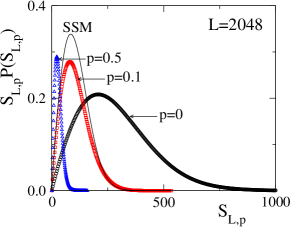
Figure 3: (Colour online) Plot of $S_{L,p}P(S_{L,p})$ versus $S_{L,p}$ for RRSM at different values of $p$ $(0.0,0.1,0.5)$ for $L=2048$. For the sake of comparison, the same distribution for the SSM is shown by a solid line.

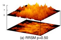
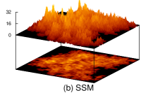
Figure 4: (Colour online) (a) Toppling surfaces of RRSM at $p=0.5$ generated on a square lattice of size $L=128$. (b) Toppling surface of the SSM generated on the same system size. The highest toppling number corresponds to a light brown colour and the lower toppling numbers are represented by darker and darker brown colours. Below each surface, their $2D$ projections are shown. These projections represent the avalanche clusters in two dimensions.

IV.1 Distribution of $S_{L,p}$ and avalanche morphology

The probability distribution of $S_{L,p}$ is defined as $P(S_{L,p})=n_{S}/A$ where $n_{S}$ is the number of sand columns that toppled $S$ times and $A$ is the number of distinct sand columns (or lattice sites) toppled. A FSS study of $P(S_{L,p})$ reported in Ahmed and Santra (2010b) suggests that RSM and SSM follow FSS, but BTW does not. In Fig. 3, distributions $S_{L,p}P(S_{L,p})$ of RRSM are plotted against $S_{L,p}$ for several values of $p$ for a fixed $L=2048$ and compared with that of the SSM. The distribution $S_{L,p}P(S_{L,p})$ is found to be of Poisson type as expected. However its height, width, and the peak position vary strongly with $p$ on a given lattice. It can also be noted that the distribution of the SSM is not identical with that of RRSM at $p=0.5$. This implies that the internal structure of an avalanche at different values of $p$ is different, but also it is different from that of the SSM in comparison to that of RRSM at $p=0.5$. The avalanche morphologies of two typical avalanches generated on a $128\times 128$ square lattice for RRSM at $0.5$ and for that of the SSM are presented in Fig. 4. The values of the toppling number at different lattice sites of an avalanche define a surface in three dimensions called toppling surface Ahmed and Santra (2010b). Thus, the height of the toppling surface at the $i$th lattice site is then given by $S_{L,p}[i]$. The toppling surface of RRSM at $p=0.5$ is found to be fluctuating all over the lattice as that of the SSM with different maximum heights. For SSM, it is approximately $31$, whereas that for RRSM at $p=0.5$ is approximately $12$, similar to the observation of their steady-state heights. The projection of the toppling surfaces in two dimensions is shown below the respective toppling surfaces. The $2D$ view of a toppling surface is known as an avalanche cluster. It can be seen that the avalanche cluster of RRSM at $p=0.5$ exhibits random mixing of colours representing different toppling numbers as that of an avalanche cluster of the SSM. Note that both are very different from that of the RSM in which a random superposition of several BTW-type concentric zones Biham et al. (2001); Grassberger and Manna (1990) of lower and lower toppling numbers around different maximal toppling zones is observed Santra et al. (2007). Since the avalanche morphologies of RRSM at $p=0.5$ and the SSM are found to be similar, it is expected that both models have the same critical behaviour, though the distributions $S_{L,p}P(S_{L,p})$ of them are different.

IV.2 Properties of avalanche size

One of the macroscopic avalanche properties is the total number of toppling in an avalanche, called the toppling size $s$. Knowing the values of $S_{L,p}[i]$ at every lattice site, the toppling size $s$ of an avalanche can be obtained as

$$s(L,p)=\sum_{i=1}^{L^{2}}S_{L,p}[i]$$ (4)

for given $L$ and $p$. At the steady state, $5\times 10^{5}$ avalanches are generated on every quenched random configuration of the toppling rules for a given value of $p$. For every value of $p$, $64$ configurations of quenched toppling rules are considered. Therefore, ensemble averaging is performed over $N_{\rm tot}=32\times 10^{6}$ avalanches for given values of $L$ and $p$. The probability to have an avalanche of toppling size $s$ is given by the $P_{L,p}(s)=N_{s}(L,p)/N_{\rm tot}$ where $N_{s}(L,p)$ is the number of avalanches of toppling size $s$ for given $L$ and $p$ out of total number of avalanches $N_{\rm tot}$ generated. For RSM (corresponding to $p=0$ and $1$ of RRSM), it is already known that the distribution of $s$ follows a power law scaling with a well defined exponent $\tau_{s}$ and obey FSS Santra et al. (2007); Ahmed and Santra (2010a). The probability distributions $P_{L,p}(s)$ for the toppling size $s$ for several values of $p$ (other than $0$ and $1$) for a fixed large system sizes $L=2048$ and for several values of $L$ for a fixed value of $p$ show that not only the cutoffs but also the slopes of the distributions depend on $p$ for a fixed $L$ whereas for a fixed $p$ only the cutoffs of the distributions depend on $L$ keeping the slopes unchanged. For a given $p$, a probability distribution function for toppling size $s$ is then proposed as

$$P_{L,p}(s)=s^{-\tau_{s}(p)}f_{p}\left[\frac{s}{L^{D_{s}(p)}}\right],$$ (5)

where $f_{p}$ is the $p$ dependent scaling function and $D_{s}(p)$ is the capacity dimension of the toppling size $s$ corresponding to given $p$. To have estimates of the exponents $\tau_{s}(p)$ and $D_{s}(p)$ defined in Eq. (5), the concept of moment analysis Karmakar et al. (2005); Lübeck (2000b) for the avalanche size $s$ has been employed. For a given $p$, the $q$th moment of $s$ as function of $L$ is obtained as

$$\langle s^{q}(L,p)\rangle = \int_{0}^{\infty}s^{q}P_{L,p}(s)ds\sim L^{\sigma_{s}(p,q)},$$ (6)

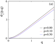
Figure 5: (Colour online) (a) Plot of $\sigma_{s}(p,q)$ against $q$ for different values of $p$. (b) The variations of $\tau_{s}(p)$ and $D_{s}(p)$ against $p$ are shown.

where the moment scaling exponent $\sigma_{s}(p,q)$ would be $\sigma_{s}(p,q)=D_{s}(p)[q+1-\tau_{s}(p)]$ for large $q$ as $q>\tau_{s}(p)-1$. For each value of $p$, a sequence of values of $\sigma_{s}(p,q)$ as a function of $q$ is determined by estimating the slope of the plots of $\log\langle s^{q}(L,p)\rangle$ versus $\log(L)$ for $200$ equidistant values of $q$ between $0$ and $2$. $\sigma_{s}(p,q)$ is plotted against $q$ for different values of $p$ in Fig. 5(a). To obtain the values of $\tau_{s}(p$) and $D_{s}(p)$, the direct method developed by Lübeck Lübeck (2000b) is employed in which a straight line is fitted through the data points for $q>\tau_{s}(p)-1$. From the straight line fitting, the $x$ intercept provides $\tau_{s}(p)-1$ and the $y$-intercept provides $D_{s}(p)[1-\tau_{s}(p)]$. Straight lines are fitted through the data points for different values of $p$ in the range of $q$ between $1$ and $2$, and the $x$ and $y$ intercepts are noted. The estimated values of the exponents $\tau_{s}(p)$ and $D_{s}(p)$ are then presented in Fig. 5(b) against $p$. There is a continuous change in the values of $\tau_{s}(p)$ and $D_{s}(p)$ as $p$ changes from $0$ to $1$. This indicates a continuous crossover of the critical behaviour of the system through a series of universality classes of RRSM at different values of $p$. The exponents $\tau_{s}(p)=1.234(13)$ and $D_{s}(p)=2.82(2)$ at $p=0$ and $1$ correspond to that of the RSM Santra et al. (2007) as expected. However, the values of the critical exponents $\tau_{s}(p)=1.286(9)$ and $D_{s}(p)=2.71(2)$ at $p=0.5$ are found very close to that of the SSM Huynh et al. (2011); Chessa et al. (1999); Lübeck (2000b). Although both of the exponents are varying continuously with $p$, due to the diffusive behaviour of RRSM, the scaling relation $D_{s}(p)[2-\tau_{s}(p)]=2$ is found to be valid within error bars for all values of $p$. It can be noted here that the continuous crossover in RRSM from one stochastic to another stochastic universality class through a series of stochastic classes is very different from the observed crossover phenomena from one deterministic to a stochastic universality class Karmakar et al. (2005); Černák (2006).

To verify the form of the scaling function $f_{p}$ given in Eq. (5), the scaled distributions $P_{L,p}(s)L^{D_{s}(p)\tau_{s}(p)}$ is plotted against the scaled variable $s/L^{D_{s}(p)}$ for four different system size $L$ for $p=0.25$ in Fig.6(a) and for $p=0.50$ in Fig. 6(b) in double logarithmic scales. It can be seen for both the cases that data for different values $L$ are collapsed onto a single curve, i.e., the scaling function. Hence, the proposed scaling function form in Eq. (5) for RRSM for any values of $p$ and $L$ is a correct scaling function form. The analysis not only provides estimates of the values of the exponents, but it also confirms that the model exhibits FSS. The steady-state event distribution of this slowly driven dynamical system is then found to obey power-law scaling at different values of $p$; RRSM then exhibits SOC for any value of $p$ with different sets of critical exponents. Moreover, at $p=0.5$ of RRSM, the appearance of SSM confirms the existence of the Manna class.

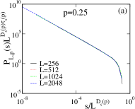
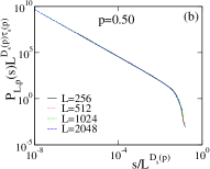
Figure 6: (Colour online) Plot of $P_{L,p}(s)L^{D_{s}(p)\tau_{s}(p)}$ against $s/L^{D_{s}(p)}$ with different values of $L$ is shown in (a) for $p=0.25$ and in (b) for $p=0.50$.

IV.3 Properties of toppling surfaces

The toppling surfaces are obtained for large spanning avalanches only. The spanning avalanches are those that are touching the opposite sides of the given lattice. For a given system size $L$, a total of $N_{\rm span}=1024$ spanning avalanches are taken over $64$ initial random configurations for each values of $p$. To study the scaling behaviour of a two-point height-height correlation function, the correlation between the toppling numbers of two lattice sites separated by a certain distance has to be determined. Since the correlation function has to be calculated as a function of a continuous variable $r$, (the distance between any two lattice sites), the toppling number of a site is represented as $S_{L,p}(x)$, where $x$ is the position vector of the lattice site with respect to the origin of a $2D$ coordinate system instead of using a discrete sequence of toppling numbers stored in $S_{L,p}[i]$. The square of the difference of toppling numbers $\delta S_{L,p}(r)$ at two lattice sites separated by a distance $r$ is given by

$$\delta S_{L,p}(r)=\left|S_{L,p}(x+r)-S_{L,p}(x)\right|^{2},$$ (7)

where $S_{L,p}(x+r)$ is the toppling number at $x+r$ for given $L$ and $p$. The probability $P[\delta S_{L,p}(r)]$ of a particular value of $\delta S_{L,p}(r)$ occurring for a particular $r$ for a given value of $L$, $p$ is defined as

$$P[\delta S_{L,p}(r)]=\frac{n_{\delta S_{L,p}(r)}}{N_{r}},$$ (8)

where $n_{\delta S_{L,p}(r)}$ is the number of pairs of sand columns having the desired value of $\delta S_{L,p}(r)$ and $N_{r}$ is the total number of pairs separated by a distance $r$ for all the surfaces. To determine $N_{r}$, for each surface $100$ centers are randomly selected. From each center, all possible sand columns at a distance $r$ are counted and then added for $N_{\rm span}=1024$ surfaces. The probability distribution $P[\delta S_{L,p}(r)]$ is then estimated for several values of $L$, $p$, and $r$. To guess the form of the distribution function $P[\delta S_{L,p}(r)]$, once is plotted against $p$ for a fixed system size $L=2048$ and $r=512$ and then it is plotted against $L$ for a fixed value of $p=0.25$ and $r=128$ in Fig. 7(a) and 7(b), respectively. It can be seen that as $p$ increases, the cutoffs of the distributions decrease for a given system size $L$. On the other hand, for a given $p$ the cutoffs increase as the system size $L$ is increased. Hence, following Ref. Alava et al. (2006); *bouchbinderPRL06; *santucciPRE07; *bakkePRE07 the form of the probability distribution function $P[\delta S(r,p,L)]$ is proposed as

$$P[\delta S_{L,p}(r)]=\frac{r^{-2H(p)}}{L^{\zeta}}g\left[\frac{\delta S_{L,p}(r)}{L^{\zeta}r^{2H(p)}}\right],$$ (9)

where $H(p)$ is the $p$-dependent Hurst exponent, $\zeta$ is another exponents, and $g$ is the scaling function.

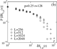
Figure 7: (a) Probability distribution of $\delta S_{L,p}(r)$ for RRSM with $p=0.10$ ($\Circle$), $0.20$ ($\Box$), $0.25$ ($\Diamond$), $0.35$ ($\triangle$), $0.50$ ($\triangleleft$) with $L=2048$ and $r=512$. (b) Distribution of $\delta S_{L,p}(r)$ for different $L$ as $L=256$ ($\Circle$), $512$ ($\Box$), $1024$ ($\Diamond$), $2048$ ($\triangle$) for fixed values of $p=0.25$ and $r=128$.

The correlation between the toppling numbers of two sand columns separated by a distance $r$ can be obtained by estimating the expectation $\langle\delta S_{L}(r,p)\rangle$. The correlation function for a given $L$ and $p$, is obtained as

$$C_{L,p}(r) = \int_{0}^{\infty}\delta S_{L,p}(r)P[\delta S_{L,p}(r)]d[\delta S_{L,p}(r)]$$ (10)

$$= r^{2H(p)}L^{\zeta}\int_{0}^{\infty}zg(z)dz$$

$$\sim r^{2H(p)}L^{\zeta}$$

where $z=\delta S_{L,p}(r)/(L^{\zeta}r^{2H(p)})$ is the scaled variable and the value of the integral would be a constant. Notice that $C_{L,p}(r)$ is a system size dependent correlation function. Such correlation functions also appear in the cases of growing interfaces in random media and self-affine fracture surfaces López (1995); *lopezPRE96; *lopezPRE98; *morelPRE98; *lopezPRL99. In order to determine the Hurst exponent $H(p)$, and the values of $\zeta$, integrated correlation function $I_{L,p}(R)$ up to a distance $R$ and the overall surface width $W_{L,p}$ are estimated. $I_{L,p}(R)$ and $W_{L,p}$ are obtained as

$$I_{L,p}(R) = \int_{0}^{R}C_{L,p}(r)dr\sim R^{1+2H(p)}L^{\zeta}$$ (11)

and

$$W^{2}_{L,p} = \frac{1}{L^{2}}\int_{0}^{L}C_{L,p}(r)rdr\sim L^{2\chi(p)},$$ (12)

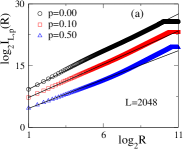
Figure 8: (Colour online) (a) Plot of $I_{L,p}(R)$ against $R$ for $p=0.0$ ($\Circle$), $p=0.10$ ($\Box$) and $p=0.50$ ($\triangle$) on a system of size $L=2048$. The straight lines represent the linear least-squares-fitted lines through the linear region of the data points. (b) Plot of $W_{L,p}$ against $L$ for the same values of $p$ as in (a) with the same symbols. The straight lines are the linear least-squares-fitted lines through the data points. In (c) and (d), $H(p)$ and $\chi(p)$ are plotted, respectively, against $p$. The dashed lines in (c) and (d) represent the values of $H$ and $\chi$ for the SSM.

where $\chi(p)=\zeta/2+H(p)$ is known as the roughness exponent. $I_{L,p}(R)$ against $R$ and $W_{L,p}$ against $L$ are plotted in double logarithmic scales in Figs. 8(a) and 8(b), respectively for the RRSM at $p=0,0.1$ and $0.5$ and for different values of $L=128-2048$. It can be seen that both $I_{L,p}(R)$ and $W_{L,p}$ follow power-law scaling with their respective arguments. The slopes are obtained by a linear least-squares fit through the data points, and one obtains $1+2H(p)$ from (a) and $\chi(p)$ from (b). The values of the Hurst exponents $H(p)$ and the roughness exponent $\chi(p)$ are plotted against $p$ in Figs. 8(c) and 8(d), respectively. A few observations are there. First, a continuous crossover in the values of the critical exponents has occurred as $p$ changed from $0$ (or $1$) to $0.5$. This confirms the existence of a series of stochastic universality classes as observed in the case of an avalanche size distribution exponent. Second, not only the values of $H(p)\approx 0.35$ and $\chi(p)\approx 0.82$ for the RRSM at $p=0$ and $1$ is found to be the same as those of the RSM Ahmed and Santra (2012a), but also the values of $H(p)\approx 0.21$ and $\chi(p)\approx 0.70$ for the RRSM at $p=0.5$ are found to be close to those of the SSM Ahmed and Santra (2012a). The dashed lines in Fig. 8(c) and 8(d) represent the values of $H$ and $\chi$ for the SSM. Therefore, the Manna class exists in the strong disordered limit of the RRSM. Third, comparing the values of $\chi(p)$ and $H(p)$ for all values $p$, it is observed that $\chi(p)\approx H(p)+1/2$, which suggests that $\zeta\approx 1$. In that case, the values of $\chi(p)$ and $H(p)$ obtained in the RRSM for different values of $p$ do not satisfy the usual Family-Vicsek scaling (no difference in the roughness exponent and the Hurst exponent) Family and Vicsek (1985), rather they satisfy an anomalous scaling given by $\chi(p)=\zeta/2+H(p)$ with $\zeta=1$ for any value of $p$. Such a scaling relation is already verified for the RSM and the SSM Ahmed and Santra (2012a, b) independently. Note that the anomalous scaling resulted here due to the system size dependence of the correlation function $C_{L,p}(r)$ Hansen and Mathiesen (2006). Finally, the critical exponent of toppling surfaces and that of the avalanche size distribution are found to be related as $D_{s}(p)=2+\chi(p)$ Ahmed and Santra (2012b) at each value of $p$. The results obtained in two different methods are then consistent.

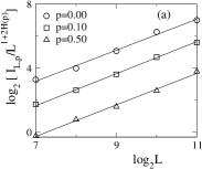
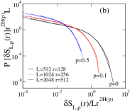
Figure 9: (Colour online) (a) Plot of $I_{L,p}/L^{1+2H(p)}$ against $L$ for different $p$. The straight line through data points gives the value of $\zeta\approx 1$. (b) Plot of $P[\delta S_{L,p}(r)]r^{2H(p)}L$ against $\delta S_{L,p}(r)/Lr^{2H(p)}$ for $p=0.0$, $p=0.1$, and $p=0.5$ for different values of $L$ and $r$ (see the legend).

To verify the scaling form of the probability distribution $P[\delta S_{L,p}(r)]$, the value of the exponent $\zeta$ must be determined. To obtain the numerical value of $\zeta$, $I_{L,p}/R^{1+2H(p)}$ for $R=L$ are plotted against $L$ for several values of $p$ in Fig.9(a). From the slopes of the linear least-squares-fitted straight lines, it is found that $\zeta\approx 1$ for all values of $p$, as already predicted by the scaling relations. The scaling function form given in Eq. (9) is now verified by plotting a scaled distribution $P[\delta S_{L,p}(r)]r^{2H(p)}L$ against a scaled variable $\delta S_{L,p}(r)/Lr^{2H(p)}$ for different values of $p$ in Fig. 9(b). For $\zeta=1$, good data collapses are observed for different values of $L$ and $r$ at three different values of $p$ with the respective values of the Hurst exponent $H(p)$. Thus the proposed scaling form assumed in Eq. (9) is correct. Such distribution functions will then be useful to analyze rough surfaces arising in a system with controlled disorder.

IV.4 Comparison of SSM and RRSM at $p=0.5$

Alhough the macroscopic parameters describing the critical states of the RRSM at $p=0.5$ and the SSM are found to be drastically different, the values of the critical exponents are found to be similar. It is then important to compare the scaling function forms of both models. The probability distributions of toppling size $s$ and that of the square difference of toppling numbers $\delta S(r)$ are considered for comparison of their associated scaling functions. The model-dependent probability distributions for $s$ and $\delta S(r)$ are proposed as

$$P_{s,m}=a_{m}s^{-\tau_{sm}}f_{m}(b_{m}s/L^{D_{sm}})$$ (13a)

and

$$P_{\delta S,m}=c_{m}r^{-2H_{m}}g_{m}[d_{m}\delta S(r)/r^{2H_{m}}],$$ (13b)

where $m$ represents the models RRSM at $p=0.5$ and the SSM, and $a_{m}$, $b_{m}$, $c_{m}$, and $d_{m}$ are non-universal metric factors that contain all non-universal model-dependent features such as the lattice structure, the update scheme, the type or range of interaction, etc. Lübeck and Heger (2003a); *lubeckPRE03. The $p$ dependence in both the functions and the $L$ dependence in Eq. (13b) are dropped because they are considered either for a fixed value of $p$ or for a fixed value of $L$. Assuming $a_{m}$, $b_{m}$ and $c_{m}$, $d_{m}$ all are equal to $1$, the scaled distributions $P_{s,m}s^{\tau_{sm}}$ for several values of $L$ and $P_{\delta S,m}r^{2H_{m}}$ for several value of $r$ for $L=2048$ are plotted in Figs. 10(a) and 10(b) respectively, against their respective scaled variables $s/L^{D_{sm}}$ and $\delta S(r)/r^{2H_{m}}$ using the same values of $\tau_{sm}$, $H_{m}$ and $D_{sm}$ for both models. It can be seen that in both cases, the distributions collapse onto two different curves corresponding to the RRSM at $p=0.5$ and the SSM. It seems that scaling functions are different for these two models, although they scale independently with their respective arguments with the same critical exponents. It is then essential to verify whether the scaling functions are affected by the non-universal metric factors or not. The values of $a_{m}$ are calculated from the limiting value of $P_{s,mL}s^{\tau_{sm}}$ as $s\rightarrow 0$, and they are found to be $a_{m}=0.34\pm 0.01$ for the RRSM at $p=0.5$ and $a_{m}=0.27\pm 0.01$ for the SSM. The values of $b_{m}$ are calculated from the average toppling numbers $s$ of the two models for a fixed $L$. For $L=2048$, the values are $b_{m}=2^{-16.92\pm 0.02}$ for the RRSM at $p=0.5$ and $b_{m}=2^{-18.65\pm 0.03}$ for the SSM. The error bars represent the uncertainty due to different independent runs. Similarly, the values of $c_{m}$ are calculated from the limiting value of $P_{\delta S,m}$ as $\delta S(r)\rightarrow 0$ for $r=1$. For the RRSM at $p=0.5$ and for the SSM, the estimated values are $c_{m}=0.60\pm 0.01$ and $0.25\pm 0.01$, respectively. The values of $d_{m}$ are essentially the inverse of the averages of the scaled variable $\langle\delta S(r)/r^{2H_{m}}\rangle$ for the respective models. The values of $d_{m}$ are $2^{-3.66\pm 0.02}$ and $2^{-6.93\pm 0.02}$ for the RRSM at $p=0.5$ and the SSM, respectively. In Fig. 10(c) and 10(d), the scaled distribution functions are plotted against their scaled variables incorporating the metric factors of the respective models for both distributions. It can be seen that a reasonable data collapse is observed in both cases. Hence, both the scaling functions $f_{sm}$ and $g_{m}$ for two models are essentially the same apart from the non-universal metric factors associated with them. Therefore, the critical state of the RRSM at $p=0.5$ belongs to the so called stochastic or Manna universality class, although the origins of such a universality class in the two models are completely different. The stochasticity in the RRSM at $p=0.5$ is due to the simultaneous presence of two conflicting toppling rules (CTR and ATR) randomly at equal proportions, whereas the stochasticity in the SSM is externally imposed through the toppling rules. This is therefore independent confirmation of the existence of the Manna universality class as it is observed in other models Lee (2013); Lee and Kim (2013) in the context of APT on a diluted lattice.

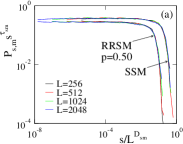
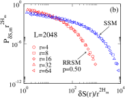
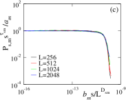
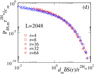
Figure 10: (Colour online) (a) Plot of scaled toppling size distributions $P_{s,m}s^{\tau_{sm}}$ of the two models RRSM at $p=0.5$ and SSM against the scaled variable $s/L^{D_{sm}}$ for different system sizes $L=256$ (black line), $512$ (red line), $1024$ (green line), and $2048$ (blue line). (b) Plot of $P_{\delta S,m}r^{2H_{m}}$ against $\delta S(r)/r^{2H_{m}}$ for different values of $r$ (see the legend) for $p=0.5$ of the RRSM and the SSM for $L=2048$. The same distributions given in (a) and (b) are plotted in (c) and (d), respectively, after normalizing by the respective non-universal metric factors.

V Conclusion

A continuous crossover from RSM to SSM (Manna class) is observed in a random rotational sandpile model as the fraction $p$ of lattice sites with the anti-clockwise toppling rule (and the rest of the lattice sites are with the clockwise toppling rule) varies from $0$ (or $1$) to $0.5$. As $p$ changes from $0$ (or $1$) to $0.5$, the system passes through a series of non-universal stochastic models at each value of $p$. Finally at $p=0.5$, at which there is maximum disorder in the toppling rule, the RRSM corresponds to the Manna class. However, not only does the origin of stochasticity in the RRSM and SSM differ, but the macroscopic parameters identifying the critical steady states of these models differ significantly as well. A scaling theory for such a continuous crossover is developed and verified numerically by estimating a set of critical exponents related to the avalanche properties as well as to that of the toppling surfaces. The values of the critical exponents satisfy all scaling relations among them for all values of $p$. This study then not only represents a continuous crossover from the RSM to the SSM, but it also confirms the existence of the Manna class at the strong disorder limit of the RRSM.

References

- Bak (1996) P. Bak, How Nature Works: The Science of Self-Organized Criticality (Copernicus, New York, 1996).
- Jensen (1998) H. J. Jensen, Self-Organized Criticality (Cambridge University Press, Cambridge, 1998).
- Pruessner (2012) G. Pruessner, Self- Organized Criticality: Theory, Models and Characterization (Cambridge University Press, Cambridge, 2012).
- Bak et al. (1987) P. Bak, C. Tang, and K. Wiesenfeld, Phys. Rev. Lett. 59, 381 (1987).
- Biham et al. (2001) O. Biham, E. Milshtein, and O. Malcai, Phys. Rev. E 63, 061309 (2001).
- Zhang (1989) Y. C. Zhang, Phys. Rev. Lett. 63, 470 (1989).
- Manna (1991a) S. S. Manna, J. Phys. A 24, L363 (1991a).
- Manna (1991b) S. S. Manna, Physica A 179, 249 (1991b).
- Dhar (1999a) D. Dhar, Physica A 270, 69 (1999a).
- Lübeck (2000a) S. Lübeck, Phys. Rev. E 62, 6149 (2000a).
- Dhar and Ramaswamy (1989) D. Dhar and R. Ramaswamy, Phys. Rev. Lett. 63, 1659 (1989).
- Marro and Dickman (1999) J. Marro and R. Dickman, Nonequilibrium Phase Transitions in Lattice Models (Cambridge University Press, Cambridge, 1999).
- Henkel et al. (2008) M. Henkel, H. Hinrichsen, and S. Lubeck, Nonequilibrium Phase Transitions, Vol. 1 (Springer, Berlin, 2008).
- Hinrichsen (2000) H. Hinrichsen, Adv. Phys. 49, 815 (2000).
- Tadić and Dhar (1997) B. Tadić and D. Dhar, Phys. Rev. Lett. 79, 1519 (1997).
- Rossi et al. (2000) M. Rossi, R. P. Satorras, and A. Vespignani, Phys. Rev. Lett. 85, 1803 (2000).
- Santra et al. (2007) S. B. Santra, S. R. Chanu, and D. Deb, Phys. Rev. E 75, 041122 (2007).
- Ahmed and Santra (2012a) J. A. Ahmed and S. B. Santra, Phys. Rev. E 85, 031111 (2012a).
- Ahmed and Santra (2010a) J. A. Ahmed and S. B. Santra, Eur. Phys. J. B 76, 13 (2010a).
- Ahmed and Santra (2011) J. A. Ahmed and S. Santra, Com. Phys. Comm. 182, 1851 (2011).
- Dickman et al. (1998) R. Dickman, A. Vespignani, and S. Zapperi, Phys. Rev. E 57, 5095 (1998).
- Muñoz et al. (1999) M. A. Muñoz, R. Dickman, A. Vespignani, and S. Zapperi, Phys. Rev. E 59, 6175 (1999).
- Vespignani et al. (2000) A. Vespignani, R. Dickman, M. A. Muñoz, and S. Zapperi, Phys. Rev. E 62, 4564 (2000).
- Bonachela et al. (2006) J. A. Bonachela, J. J. Ramasco, H. Chaté, I. Dornic, and M. A. Muñoz, Phys. Rev. E 74, 050102 (2006).
- Bonachela and Muñoz (2007) J. A. Bonachela and M. A. Muñoz, Physica A 384, 89 (2007).
- Bonachela and Muñoz (2008) J. A. Bonachela and M. A. Muñoz, Phys. Rev. E 78, 041102 (2008).
- Lee (2013) S. B. Lee, Phys. Rev. Lett. 110, 159601 (2013).
- Lee and Kim (2013) S. B. Lee and J. S. Kim, Phys. Rev. E 87, 032117 (2013).
- Lee (2014a) S. B. Lee, Phys. Rev. E 89, 062133 (2014a).
- Lee (2014b) S. B. Lee, Phys. Rev. E 89, 060101 (2014b).
- Mohanty and Dhar (2002) P. K. Mohanty and D. Dhar, Phys. Rev. Lett. 89, 104303 (2002).
- Mohanty and Dhar (2007) P. Mohanty and D. Dhar, Physica A 384, 34 (2007).
- Basu et al. (2012) M. Basu, U. Basu, S. Bondyopadhyay, P. K. Mohanty, and H. Hinrichsen, Phys. Rev. Lett. 109, 015702 (2012).
- Dhar (1999b) D. Dhar, Physica A 263, 4 (1999b), and references therein.
- Dhar (2006) D. Dhar, Physica A 369, 29 (2006).
- Karmakar et al. (2005) R. Karmakar, S. S. Manna, and A. L. Stella, Phys. Rev. Lett. 94, 088002 (2005).
- Pradhan and Chakrabarti (2001) S. Pradhan and B. K. Chakrabarti, Phys. Rev. E 65, 016113 (2001).
- Ahmed and Santra (2010b) J. A. Ahmed and S. B. Santra, Europhys. Lett. 90, 50006 (2010b).
- Grassberger and Manna (1990) P. Grassberger and S. S. Manna, J. Phys (France) 51, 1077 (1990).
- Lübeck (2000b) S. Lübeck, Phys. Rev. E 61, 204 (2000b).
- Huynh et al. (2011) H. Huynh, G. Pruessner, and L. Chew, J. Stat. Mech 2011, P09024 (2011).
- Chessa et al. (1999) A. Chessa, H. E. Stanley, A. Vespignani, and S. Zapperi, Phys. Rev. E 59, R12 (1999).
- Černák (2006) J. Černák, Phys. Rev. E 73, 066125 (2006).
- Alava et al. (2006) M. J. Alava, P. K. V. V. Nukala, and S. Zapperi, J. Stat. Mech 2006, L10002 (2006).
- Bouchbinder et al. (2006) E. Bouchbinder, I. Procaccia, S. Santucci, and L. Vanel, Phys. Rev. Lett. 96, 055509 (2006).
- Santucci et al. (2007) S. Santucci, K. J. Måløy, A. Delaplace, J. Mathiesen, A. Hansen, J. O. Haavig Bakke, J. Schmittbuhl, L. Vanel, and P. Ray, Phys. Rev. E 75, 016104 (2007).
- Haavig Bakke and Hansen (2007) J. O. Haavig Bakke and A. Hansen, Phys. Rev. E 76, 031136 (2007).
- López (1995) J. M. López, Phys. Rev. E 52, R1296 (1995).
- López and Rodríguez (1996) J. M. López and M. A. Rodríguez, Phys. Rev. E 54, R2189 (1996).
- López and Schmittbuhl (1998) J. M. López and J. Schmittbuhl, Phys. Rev. E 57, 6405 (1998).
- Morel et al. (1998) S. Morel, J. Schmittbuhl, J. M. López, and G. Valentin, Phys. Rev. E 58, 6999 (1998).
- López (1999) J. M. López, Phys. Rev. Lett. 83, 4594 (1999).
- Family and Vicsek (1985) F. Family and T. Vicsek, J. Phys. A 18, L75 (1985).
- Ahmed and Santra (2012b) J. A. Ahmed and S. Santra, Physica A 391, 5332 (2012b).
- Hansen and Mathiesen (2006) A. Hansen and J. Mathiesen, in Modeling Critical and Catastrophic Phenomena in Geoscience: A Statistical Physics Approach, edited by P. Bhattacharyya and B. K. Chakrabarti (Springer, Berlin, 2006).
- Lübeck and Heger (2003a) S. Lübeck and P. C. Heger, Phys. Rev. Lett. 90, 230601 (2003a).
- Lübeck and Heger (2003b) S. Lübeck and P. C. Heger, Phys. Rev. E 68, 056102 (2003b).