Cycle connectivity and pseudoconcavity
of flag domains

Abstract.

We prove that a non-classical flag domain is pseudoconcave if it satisfies a certain condition on the root system. Moreover, we prove that every point in a codimension-one real boundary orbit of a non-classical period domains is a pseudoconcave boundary point if it satisfies a certain Hodge-theoretical condition.

1. Introduction

Flag domains are open real group orbits in flag manifolds. The simplest example of flag domain is open orbits in $\mathbb{P}^{1}(\mathbb{C})$. The projective line $\mathbb{P}^{1}(\mathbb{C})$ is a flag manifold with the holomorphic action of $SL(2,\mathbb{C})$, which has the three real forms $SL(2,\mathbb{R})$, $SU(1,1)$, and $SU(2)$. Here the upper/lower-half planes are open $SL(2,\mathbb{R})$-orbits, the unit disks around $0$ and $\infty$ are open $SU(1,1)$-orbits, and $\mathbb{P}^{1}(\mathbb{C})$ itself is the $SU(2)$-orbit. In general, there are finitely many open real group orbits in flag manifolds, and study on flag domains has been developed by complex geometers (cf. [FHW]). Flag domains are classified into two kinds; classical or non-classical. Here we say a flag domain is non-classical if it has no non-constant holomorphic function. A classical flag domain is almost like a Hermitian symmetric domain and is well-studied, however a non-classical one is not. In this paper, we investigate non-classical flag domains. In particular, we focus on their cycle connectivity and pseudoconcavity.

Cycle connectivity of flag domains are investigated by Huckleberry [Huc2] and Green, Robles and Toledo [GRT]. We recall it briefly. Let $\check{D}$ be a flag manifold with a holomorphic action of a connected complex semisimple Lie group $G$. Let $D$ be an open $G_{\mathbb{R}}$-orbit contained in $\check{D}$ with a real form $G_{\mathbb{R}}$. For a base point $o\in D$, we have the parabolic subgroup $P$ of $G$ stabilizing $o$ and $G_{\mathbb{R}}\cap P$ contains a $\theta$-stable fundamental Cartan subgroup with a Cartan involution $\theta$. For the maximal compact subgroup $K_{\mathbb{R}}$ fixed by $\theta$, the $K_{\mathbb{R}}$-orbit $C_{0}=K_{\mathbb{R}}o$ is a compact submanifold contained in $D$. A flag domain $D$ is non-classical if and only if any two points of $D$ are connected by a connected chain $g_{1}C_{0}\cup\cdots\cup g_{\ell}C_{0}$ contained in $D$ with $g_{1},\ldots,g_{\ell}\in G$.

The other property we discuss in this paper is pseudoconcavity. We say $D$ is pseudoconcave if $D$ contains a relatively compact subset where a Levi form on every boundary point has at least one negative eigenvalue. Pseudoconcavity of complex manifolds is studied by Andreotti and Grauert in 1960’s. Pseudoconcave manifolds are a generalization of compact complex manifolds, which behave like compact complex manifolds in many ways. For instance, if $D$ is pseudoconcave, $H^{0}(D,\mathcal{O})=\mathbb{C}$ and $\mathop{\mathrm{dim}}\nolimits{H^{0}(D,E)}<\infty$ (the finiteness theorem) for any holomorphic vector bundle $E$. Moreover, the field of all meromorphic functions on a pseudoconcave manifold $D$ is an algebraic field of transcendental degree less than $\mathop{\mathrm{dim}}\nolimits{D}$. Huckleberry [Huc1] proved that classical flag domains are not pseudoconcave but pseudoconvex.

Cycle connectivity and pseudoconcavity are closely related. Huckleberry introduced one-connectivity in [Huc1]. One-connectivity is cycle connectivity in a strong sense, which requires that any two points are connected by a single cycle $gC_{0}$ with some $g\in G$. He showed that $D$ is pseudoconcave if $D$ is generically one-connected. For example, $D$ is generically one-connected if $G_{\mathbb{R}}=SL(n,\mathbb{R})$, however we do not completely know what kind of flag domain this property holds. In [GGK2, Lecture 10], Green, Griffiths and Kerr examined pseudoconcavity of the Carayol domain (Example 3.8) by an argument about boundary behavior of its cycle space. On the other hand, Kollár [Ko] proved the finiteness theorem for every non-classical flag domains by using their cycle connectivity without pseudoconcavity. Huckleberry conjectured that any non-classical flag domain is pseudoconcave.

Our purpose of this paper is to give a sufficient condition for non-classical flag domains to be pseudoconcave, which [Huc1] did not reach. In the Lie algebra level, we have the $\theta$-stable Cartan subalgebra $\mathfrak{h}_{\mathbb{R}}\subset\mathfrak{g}_{\mathbb{R}}\cap\mathfrak{p}$ and the maximal compact subalgebra $\mathfrak{k}_{\mathbb{R}}$ fixed by $\theta$. Let $\Delta$ be the set of roots. Then we have the graded Lie algebra decomposition $\mathfrak{g}=\mathfrak{g}^{-k}\oplus\cdots\oplus\mathfrak{g}^{k}$ defined by a subset of the simple roots such that $\mathfrak{p}=\bigoplus_{\ell\geq 0}\mathfrak{g}^{\ell}$. We say a root $\alpha\in\Delta$ is compact (resp. non-compact) if $\alpha\in\Delta(\mathfrak{k})$ (resp. $\alpha\in\Delta(\mathfrak{k}^{\perp})$).

Theorem 1.1.

Suppose that there exist a compact root $\beta$ such that for any non-compact root $\alpha$ in $\Delta(\mathfrak{g}^{<0})$ the $\beta$-string containing $\alpha$ is one of the following:

• $\{\alpha,\alpha+\beta\}$ with $\alpha+\beta\in\Delta(\mathfrak{p})$;

• $\{\alpha,\alpha+\beta,\alpha+2\beta\}$ with $\alpha+2\beta\in\Delta(\mathfrak{p})$.

Then $D$ is pseudoconcave.

Our study is motivated by Hodge theory. A rational Hodge structure defines a rational algebraic group called a Mumford–Tate group, and an orbit of a real Mumford–Tate group is called a Mumford–Tate domain, which is a measurable flag domain (cf. [GGK1]). For example, a period domain (cf. [CG]) is a Mumford–Tate domain of a special kind. We give two examples of Mumford–Tate domain where the above theorem holds (Example 3.8–3.9).

In the latter half of this paper, we discuss pseudoconcavity at a boundary point of $D$ in a real codimension-one $G_{\mathbb{R}}$-orbit for a non-classical period domain $D$. In this case $G_{\mathbb{R}}$ is $Sp(2n)$ or $SO(p,q)$ depending on its Hodge numbers. Now the boundary $\mathrm{bd}{(D)}$ in $\check{D}$ is the disjoint union of finitely many boundary $G_{\mathbb{R}}$-orbits. For a real codimension-one $G_{\mathbb{R}}$-orbit $\mathcal{O}$, we may consider a Levi form and define pseudoconcavity at a point in $\mathcal{O}$. By transitivity of $G_{\mathbb{R}}$ acting on $D$, every point in $\mathcal{O}$ is pseudoconcave boundary point of $D$ if one point in $\mathcal{O}$ is. We then say a codimension-one $G_{\mathbb{R}}$-orbit $\mathcal{O}$ is a pseudoconcave boundary orbit of $D$ if a point in $\mathcal{O}$ is pseudoconcave boundary point of $D$.

Boundary $G_{\mathbb{R}}$-orbits have a relationship with degeneration of Hodge structures. By the nilpotent orbit theorem [S], degenerating Hodge structures over a product of punctured disks are asymptotically approximated by nilpotent orbits. A nilpotent orbit is generated by a pair consisting of $N\in\mathfrak{g}_{\mathbb{R}}$ and $F^{\bullet}\in\check{D}$, and the limit point $\lim_{\mathop{\mathrm{Im}}\nolimits{(z)}\to\infty}\exp{(zN)}=:F^{\bullet}_{\infty}\in\check{D}$, which is called the reduced limit, is in a boundary $G_{\mathbb{R}}$-orbit. A boundary $G_{\mathbb{R}}$-orbit is said to be poralizable if it is a $G_{\mathbb{R}}$-orbit of a reduced limit. Remark that not every boundary $G_{\mathbb{R}}$-orbits are polarizable.

Green, Griffiths and Kerr [GGK2] and Kerr and Pearlstein [KP] showed that any codimension-one boundary $G_{\mathbb{R}}$-orbit $\mathcal{O}$ is polarizable. We then have a nilpotent orbit $(N,F^{\bullet})$ so that the reduced limit $F^{\bullet}_{\infty}$ is in $\mathcal{O}$, which is called a minimal degeneration. Minimal degenerations are studied by Green, Griffiths and Robles [GGR]. In Theorem 4.4, we will give a sufficient condition of $(N,F^{\bullet})$ for $\mathcal{O}$ to be a pseudoconcave boundary orbit examining minimal degenerations.

In this paper, we do not deal with degree of pseudoconcavity, and we leave it open. If a flag domain $D$ is $q$-pseudoconcave in the sense of Andreotti-Grauert, we have the finiteness theorem for cohomology groups of degree less than $\mathop{\mathrm{dim}}\nolimits{D}-q-1$ with locally free sheaves. In addition, it is speculated that the finiteness theorem is true for degree less than $\mathop{\mathrm{dim}}\nolimits{C_{0}}$ in [GGK2, Lecture 10] as an open question.

2. Pseudoconcavity of complex manifolds

We recall pseudoconcavity of complex manifolds following [A]. Let $\Omega$ be an open subset of $\mathbb{C}^{n}$ with a smooth boundary. For every point $z_{0}$ in the boundary $\mathrm{bd}{(\Omega)}$, we can find a neighborhood $U_{z_{0}}$ of $z_{0}$ and a $C^{\infty}$-function $\phi:U_{z_{0}}\to\mathbb{R}$ such that

$$(\mathrm{d}\phi)_{z_{0}}\neq 0,\quad\Omega\cap U_{z_{0}}=\{z\in U_{z_{0}}\;|\;\phi(z)<\phi(z_{0})\}.$$

The real tangent plane at $z_{0}$ to $\mathrm{bd}{(\Omega)}$ contains the $(n-1)$-dimensional complex plane defined by the equation

$$\sum_{k}\frac{\partial\phi}{\partial z^{k}}(z_{0})(z^{k}-z_{0}^{k})=0$$

with the coordinate function $z^{1},\ldots,z^{n}$. This is called the analytic tangent plane. Since $\phi$ is real-valued, the quadratic form

$$L(\phi)_{z_{0}}(z):=\sum_{k,\ell}\frac{\partial^{2}\phi}{\partial z^{k}\partial\bar{z}^{\ell}}(z_{0})z^{k}\bar{z}^{\ell},$$

is Hermitian, which is called the Levi form. The boundary point $z_{0}$ is said to be pseudoconcave if the Levi form has at least one negative eigenvalue on the analytic tangent plane. Remark that the number of positive/negative eigenvalues does not depend on the choice of coordinate function and defining function. We may assume $z_{0}=0$ and $\phi(0)=0$, and we may change the coordinate so that the Tayler expansion of $\phi$ at $0$ is

$$\phi(z)=2\mathop{\mathrm{Re}}\nolimits(z^{1})+L_{0}(\phi)(z)+O(\|z\|^{3})$$

and the Levi form restricted to the analytic tangent plane $T_{0}(\mathrm{bd}{(\Omega)})$, defined by $z^{1}=0$, is

$$L(\phi)_{0}|_{T_{0}(\mathrm{bd}{(\Omega)})}(z)=\sum_{k\geq 2}^{n}\lambda_{k}|z^{k}|^{2}$$

with eigenvalues $\lambda_{2},\ldots,\lambda_{n}$. If $0$ is a pseudoconcave boundary point, we have at least one negative eigenvalue, then we have a holomorphic map $\rho:\mathbb{D}\to\mathrm{c\ell}{(\Omega)}$ from the unit disk such that $\rho(0)=0$ and $\mathrm{bd}{(\rho(\mathbb{D}))}\subset\Omega$. On the other hand, if $0$ is not a pseudoconcave boundary point, we do not have such a holomorphic map. We then define pseudoconcavity of complex manifolds as follows:

Definition 2.1.

Let $X$ be a connected complex manifold. We say $X$ is pseudoconcave if there exists a relatively compact open subset $U$ with a smooth boundary such that at every point $z\in\mathrm{bd}{(U)}$ a holomorphic map $\rho:\mathbb{D}\to\mathrm{c\ell}{(U)}$ where $\rho(0)=z$ and $\mathrm{bd}{(\rho(\mathbb{D}))}\subset U$ exists.

Example 2.2.

1. Every compact complex connected manifold is pseudoconcave.

2. Let $Z$ be a compact complex connected manifold of dimension greater than $2$ and let $Y$ be a complex submanifold with $\mathop{\mathrm{dim}}\nolimits{Y}\leq\mathop{\mathrm{dim}}\nolimits{Z}-2$. Then $Z-Y$ is pseudoconcave.

3. Flag domains

We review flag domains and their root structure, and then we prove Theorem 1.1. This proof is based on technique of [Huc1, §3.2]. The key point of Huckleberry’s proof is to construct a relatively compact neighborhood of the base cycle $C_{0}$ which is filled out by cycles and where any points are one-connected to $C_{0}$. We construct such a neighborhood in Lemma 3.7. Here Cayley transform associated with compact root plays important role.

3.1. Parabolic subalgebras

Let $\mathfrak{g}$ be a complex semisimple Lie algebra, and let $\mathfrak{p}$ be a parabolic subgroup. Let $\mathfrak{g}_{\mathbb{R}}$ be a real form of $\mathfrak{g}$. We fix a Cartan subalgebra $\mathfrak{h}_{\mathbb{R}}\subset\mathfrak{g}_{\mathbb{R}}\cap\mathfrak{p}$ and choose a Borel subgroup $\mathfrak{b}\subset\mathfrak{p}$ containing the Cartan subgroup $\mathfrak{h}:=\mathfrak{h}_{\mathbb{R}}\otimes\mathbb{C}$. The Cartan subalgebra $\mathfrak{h}$ determines a set $\Delta=\Delta(\mathfrak{g},\mathfrak{h})\subset\mathfrak{h}^{*}$ of roots. A root $\alpha\in\Delta$ defines the root space $\mathfrak{g}^{\alpha}$, and we have the root space decomposition $\mathfrak{g}=\mathfrak{h}\oplus\bigoplus_{\alpha\in\Delta}\mathfrak{g}^{\alpha}$. For a subalgebra $\mathfrak{s}$, we denote by $\Delta(\mathfrak{s})$ the subset of roots of which root spaces contained in $\mathfrak{s}$. The Borel subalgebra $\mathfrak{b}$ defines a positive root system by

$$\Delta^{+}:=\Delta(\mathfrak{b})=\{\alpha\in\Delta\;|\;\mathfrak{g}^{\alpha}\subset\mathfrak{b}\}.$$

Let $\mathcal{S}=\{\sigma_{1},\ldots,\sigma_{r}\}$ be the set of simple roots, and let $\{\mathtt{S}^{1},\ldots,\mathtt{S}^{r}\}$ be the dual basis to $\mathcal{S}$. An integral linear combination $\mathtt{E}=\sum_{j}n_{j}\mathtt{S}^{j}$ is called a grading element. The $\mathtt{E}$-eigenspaces

$$\mathfrak{g}^{\ell}=\bigoplus_{\alpha(\mathtt{E})=\ell}\mathfrak{g}^{\alpha},\quad\mathfrak{g}^{0}=\mathfrak{h}\oplus\bigoplus_{\alpha(\mathtt{E})=0}\mathfrak{g}^{\alpha}$$

determines a graded Lie algebra decomposition $\mathfrak{g}=\mathfrak{g}^{-k}\oplus\cdots\oplus\mathfrak{g}^{k}$ in the sense that $[\mathfrak{g}^{\ell},\mathfrak{g}^{m}]\subset\mathfrak{g}^{\ell+m}$. A grading $\mathtt{E}$ defines a parabolic subalgebra $\mathfrak{p}_{\mathtt{E}}=\bigoplus_{\ell\geq 0}\mathfrak{g}^{\ell}$. On the other hand, setting

$$I(\mathfrak{p})=\{i\;|\;\mathfrak{g}^{-\sigma_{i}}\not\subset\mathfrak{p}\},$$

the parabolic subalgebra $\mathfrak{p}_{\mathtt{E}}$ defined by $\mathtt{E}=\sum_{i\in I(\mathfrak{p})}\mathtt{S}^{i}$ coincides with $\mathfrak{p}$.

We review Chevalley basis and their properties (cf. [Hum, §25]). Since the Killing form defines a non-degenerate negative-definite symmetric form on $\mathfrak{h}_{\mathbb{R}}$, we have the induced form $(\bullet,\bullet)$ on $\mathfrak{h}_{\mathbb{R}}^{*}$. Let $\alpha\in\Delta\cup\{0\}$ and let $\beta\in\Delta$. The set of all members of $\Delta\cup\{0\}$ of the form $\alpha+n\beta$ for $n\in\mathbb{Z}$ is called the $\beta$-string containing $\alpha$. Then the $\beta$-string containing $\alpha$ is given by

(3.1) $$\{\alpha+n\beta\;|\;-r\leq n\leq q\}.$$

If $\alpha$ and $\beta$ are linearly independent, we have

$$\langle\alpha,\beta\rangle:=2\frac{(\alpha,\beta)}{(\beta,\beta)}=r-q.$$

We can choose $\mathtt{H}^{\alpha}\in\mathfrak{h}$ and $x^{\alpha}\in\mathfrak{g}^{\alpha}$ for all $\alpha\in\Delta$ satisfying

$$[x^{\alpha},x^{-\alpha}]=\mathtt{H}^{\alpha},\quad[\mathtt{H}^{\beta},x^{\alpha}]=\langle\alpha,\beta\rangle x^{\alpha},$$

$$[x^{\alpha},x^{\beta}]=\begin{cases}c_{\alpha,\beta}x^{\alpha+\beta}&\text{if }\alpha+\beta\in\Delta\\ 0&\text{if }\alpha+\beta\not\in\Delta\end{cases}$$

$$\text{where }c_{\alpha,\beta}=-c_{-\alpha,-\beta}\in\mathbb{Z}.$$

Here $c_{\beta,\alpha}=\pm(r+1)$ if $\alpha$ and $\beta$ are linearly independent and $\alpha+\beta\in\Delta$. Now

$$\{x^{\alpha}\;|\;\alpha\in\Delta\}\cup\{\mathtt{H}^{\sigma}\;|\;\sigma\in\mathcal{S}\}$$

is a basis of $\mathfrak{g}$, which is called a Chevalley basis.

Lemma 3.1 ([Hum, §25.2]).

If $\alpha$ and $\beta$ are linearly independent, then

$$[x^{-\beta},[x^{\beta},x^{\alpha}]]=q(r+1)x^{\alpha}$$

where $(r,q)$ is given by the form (3.1).

Example 3.2 ($\mathfrak{g}=\mathfrak{sl}_{2}(\mathbb{C})$).

A basis of $\mathfrak{g}_{\mathbb{R}}=\mathfrak{sl}_{2}(\mathbb{R})$ is given by

$$x^{\alpha}=\begin{pmatrix}0&1\\ 0&0\end{pmatrix},\quad\mathtt{H}^{\alpha}=\begin{pmatrix}1&0\\ 0&-1\end{pmatrix},\quad x^{-\alpha}=\begin{pmatrix}0&0\\ 1&0\end{pmatrix}.$$

Here $\mathfrak{h}=\mathbb{C}\mathtt{H}^{\alpha}$ is a Cartan subalgebra, and $x^{\pm\alpha}$ is in the root space $\mathfrak{g}^{\pm\alpha}$ where $\alpha$ is the root given by $\alpha(\mathtt{H}^{\alpha})=2$. This triple satisfies

(3.2) $$[x^{\alpha},x^{-\alpha}]=\mathtt{H}^{\alpha},\quad[\mathtt{H}^{\alpha},x^{\alpha}]=2x^{\alpha},\quad[\mathtt{H}^{\alpha},x^{-\alpha}]=-2x^{-\alpha}.$$

In this case, $\Delta=\{\pm\alpha\}$ and we set $\alpha$ as a positive root. We define a grading $\mathtt{E}=\mathtt{S}$ where $\mathtt{S}$ is the dual of $\alpha$. Then

$$\mathfrak{g}^{1}=\mathfrak{g}^{\alpha},\quad\mathfrak{g}^{0}=\mathfrak{h},\quad\mathfrak{g}^{-1}=\mathfrak{g}^{-\alpha},$$

and $\mathfrak{p}_{\mathtt{E}}=\mathfrak{g}^{1}\oplus\mathfrak{g}^{0}$.

In general, a triple in a semisimple Lie algebra satisfying (3.2) is called a standard $sl_{2}$-triple.

3.2. Flag domains and Cayley transforms

In the Lie group level, we have the parabolic subgroup $P\subset G$ corresponding to $\mathfrak{p}\subset\mathfrak{g}$. The homogeneous manifold $\check{D}=G/P$ is called a flag manifold. We fix a Cartan involution of $\mathfrak{g}_{\mathbb{R}}$. Let $\mathfrak{p}_{x}$ be the Lie algebra of the parabolic subgroup $P_{x}$ of $G$ stabilizing $x\in\check{D}$. By [FHW, Theorem 4.2.2], the $G_{\mathbb{R}}$-orbit $G_{\mathbb{R}}x$ is open if and only if $\mathfrak{p}_{x}=\mathfrak{p}_{\mathtt{E}}$ where

• $\mathfrak{g}_{\mathbb{R}}\cap\mathfrak{p}_{x}$ contains a fundamental Cartan subalgebra $\mathfrak{h}_{\mathbb{R}}$, and

• $\mathtt{E}$ is an integral linear combination of a set of simple roots for a system $\Delta^{+}\subset\Delta=\Delta(\mathfrak{g},\mathfrak{h})$ with $\mathfrak{h}=\mathfrak{h}_{\mathbb{R}}\otimes\mathbb{C}$ such that $\tau\Delta^{+}=-\Delta^{+}$ for the complex conjugation $\tau$.

An open $G_{\mathbb{R}}$-orbit is called a flag domain. Let $D$ be a flag domain contained in $\check{D}$, and fix a base point $o\in D$. We may assume $\mathfrak{p}=\mathfrak{p}_{o}$. There exists a fundamental Cartan subalgebra $\mathfrak{h}_{\mathbb{R}}\subset\mathfrak{g}_{\mathbb{R}}\cap\mathfrak{p}$, a positive root system $\Delta^{+}$, and a grading $\mathtt{E}$ such that $\mathfrak{p}=\mathfrak{p}_{\mathtt{E}}$. We may choose a Chevalley basis of $\mathfrak{g}$. We define the Cayley transform $\mathbf{c}_{\alpha}$ for $\alpha\in\Delta$ by

$$\mathbf{c}_{\alpha}=\exp{(\frac{\pi}{4}(x^{-\alpha}-x^{\alpha}))}.$$

Remark 3.3.

Usually, Cayley transforms of the above form are defined for noncompact imaginary roots as [Kn, §VI.7]. We use a Cayley transform for a compact root in the proof of Theorem 1.1.

Example 3.4 ($\mathfrak{g}=\mathfrak{sl}_{2}(\mathbb{C})$).

This is continuation of Example 3.2. Let us consider the three real forms $\mathfrak{su}(2)$, $\mathfrak{su}(1,1)$, and $\mathfrak{sl}(2,\mathbb{R})$ of $\mathfrak{sl}(2,\mathbb{C})$. We set

$$u^{\alpha}:=x^{\alpha}-x^{-\alpha}=\begin{pmatrix}0&1\\ -1&0\end{pmatrix},\quad h^{1}:=\mathbf{i}\mathtt{H}^{\alpha}=\mathbf{i}\begin{pmatrix}1&0\\ 0&-1\end{pmatrix},$$

$$v^{\alpha}:=\mathbf{i}(x^{\alpha}+x^{-\alpha})=\mathbf{i}\begin{pmatrix}0&1\\ 1&0\end{pmatrix},$$

where $\mathbf{i}=\sqrt{-1}$. Then

$$\mathfrak{su}(2)=\mathbb{R}u^{\alpha}+\mathbb{R}h^{1}+\mathbb{R}v^{\alpha},\quad\mathfrak{su}(1,1)=\mathbb{R}\mathbf{i}u^{\alpha}+\mathbb{R}h^{1}+\mathbb{R}\mathbf{i}v^{\alpha},$$

$$\mathfrak{sl}(2,\mathbb{R})=\mathbb{R}x^{\alpha}+\mathbb{R}\mathtt{H}^{\alpha}+\mathbb{R}x^{-\alpha}=\mathbb{R}(u_{\alpha}-\mathbf{i}v_{\alpha})+\mathbb{R}\mathbf{i}h^{1}+\mathbb{R}(u_{\alpha}+\mathbf{i}v_{\alpha}).$$

The $G$-orbit $\check{D}$ is $\mathbb{P}^{1}(\mathbb{C})$ in this case. Each real group orbits of $o=\begin{pmatrix}1\\ 0\end{pmatrix}\in\check{D}$ are

$$\mathbb{P}^{1}(\mathbb{C}),\quad\left\{\begin{pmatrix}1\\ z\end{pmatrix}\;;\;|z|<1\right\},\quad\left\{\begin{pmatrix}1\\ y\end{pmatrix}\;;\;y\in\mathbb{R}\right\}\cup\left\{\begin{pmatrix}0\\ 1\end{pmatrix}\right\}.$$

In a case where $\mathfrak{g}_{\mathbb{R}}$ is $\mathfrak{su}(2)$ or $\mathfrak{su}(1,1)$, the Cartan subalgebra $\mathfrak{h}_{\mathbb{R}}=\mathfrak{p}\cap\mathfrak{g}_{\mathbb{R}}=\mathbb{R}h^{1}$ is compact and $\tau x^{\alpha}=x^{-\alpha}$ for the complex conjugate $\tau$. On the other hand, in the case where $\mathfrak{g}_{\mathbb{R}}$ is $\mathfrak{sl}(2,\mathbb{R})$, the Cartan subalgebra $\mathfrak{h}_{\mathbb{R}}=\mathfrak{p}\cap\mathfrak{g}_{\mathbb{R}}=\mathbb{R}\mathbf{i}h^{1}$ is noncompact and $\tau x^{\alpha}=x^{\alpha}$. The Cayley transform for $\alpha$ is

$$\mathbf{c}_{\alpha}=\frac{1}{\sqrt{2}}\begin{pmatrix}1&-1\\ 1&1\end{pmatrix}.$$

We then have

$$\mathbf{c}_{\alpha}(o)=\begin{pmatrix}1\\ 1\end{pmatrix},\quad\mathbf{c}^{2}_{\alpha}(o)=\begin{pmatrix}0\\ 1\end{pmatrix}.$$

Proposition 3.5.

If $\alpha$ and $\beta$ are linearly independent, then

$$\mathop{\mathrm{Ad}}\nolimits{(\mathbf{c}_{-\beta}^{2})}x^{\alpha}=\begin{cases}\pm x^{\alpha+\beta}&\text{if }(r,q)=(0,1),\\ \pm x^{\alpha+2\beta}&\text{if }(r,q)=(0,2)\end{cases}$$

where $(r,q)$ is given by the form (3.1).

Proof..

First, we consider the case for $(r,q)=(0,1)$. Since $\alpha-\beta\not\in\Delta$,

$$\mathop{\mathrm{ad}}\nolimits{(x^{\beta}-x^{-\beta})}x^{\alpha}=\mathop{\mathrm{ad}}\nolimits{(x^{\beta})}x^{\alpha}=c_{\beta,\alpha}x^{\alpha+\beta}.$$

By Lemma 3.1,

$$[x^{-\beta},[x^{\beta},x^{\alpha}]]=x^{\alpha}.$$

Then

$$(\mathop{\mathrm{ad}}\nolimits{(x^{\beta}-x^{-\beta})})^{2}x^{\alpha}=-[x^{-\beta},[x^{\beta},x^{\alpha}]]=-x^{\alpha}.$$

Therefore

$$\mathop{\mathrm{Ad}}\nolimits{(\exp{(\frac{\pi}{2}(x^{\beta}-x^{-\beta}))})}x^{\alpha} =\sum_{\ell=0}^{\infty}\frac{(-1)^{2\ell}}{(2\ell)!}(\frac{\pi}{2})^{2\ell}x^{\alpha}+\sum_{k=0}^{\infty}\frac{(-1)^{k}}{(2k+1)!}(\frac{\pi}{2})^{2k+1}c_{\beta,\alpha}x^{\alpha+\beta}$$

$$=\cos{(\frac{\pi}{2})}x^{\alpha}+\sin{(\frac{\pi}{2})}c_{\beta,\alpha}x^{\alpha+\beta}=c_{\beta,\alpha}x^{\alpha+\beta}$$

Since $c_{\beta,\alpha}=\pm 1$, the equation holds.

Next, we consider the case for $(r,q)=(0,2)$. As is the case for $(r,q)=(0,1)$, we have

$$\mathop{\mathrm{ad}}\nolimits{(x^{\beta}-x^{-\beta})}x^{\alpha}=c_{\beta,\alpha}x^{\alpha+\beta},\quad[x^{-\beta},[x^{\beta},x^{\alpha}]]=2x^{\beta}.$$

Then

$$(\mathop{\mathrm{ad}}\nolimits{(x^{\beta}-x^{-\beta})})^{2}x^{\alpha}=c_{\beta,\alpha+\beta}c_{\beta,\alpha}x^{\alpha+2\beta}-2x^{\alpha}.$$

By Lemma 3.1,

$$[x^{\beta},[x^{-\beta},x^{\alpha+2\beta}]]=2x^{\alpha+2\beta}.$$

On the other hand,

$$[x^{\beta},[x^{-\beta},x^{\alpha+2\beta}]]=c_{\beta,\alpha+\beta}c_{-\beta,\alpha+2\beta}x^{\alpha+2\beta}.$$

Then $c_{\beta,\alpha+\beta}c_{-\beta,\alpha+2\beta}=2$. Therefore,

$$(\mathop{\mathrm{ad}}\nolimits{(x^{\beta}-x^{-\beta})})^{3}x^{\alpha}=-c_{-\beta,\alpha+2\beta}c_{\beta,\alpha+\beta}c_{\beta,\alpha}x^{\alpha+\beta}-2c_{\beta,\alpha}x^{\alpha+\beta}=-4c_{\beta,\alpha}x^{\alpha+\beta}.$$

To summarize the above calculations, we have

$$\mathop{\mathrm{Ad}}\nolimits{(\exp{(\frac{\pi}{2}(x^{\beta}-x^{-\beta}))})}x^{\alpha}=x^{\alpha} +\sum_{k=0}^{\infty}\frac{1}{(2k+1)!}(\frac{\pi}{2})^{2k+1}(-4)^{k}c_{\beta,\alpha}x^{\alpha+\beta}$$

$$+\sum_{\ell=1}^{\infty}\frac{1}{(2\ell)!}(\frac{\pi}{2})^{2\ell}(-4)^{\ell-1}(c_{\beta,\alpha+\beta}c_{\beta,\alpha}x^{\alpha+2\beta}-2x^{\alpha}),$$

where

$$\sum_{k=0}^{\infty}\frac{1}{(2k+1)!}(\frac{\pi}{2})^{2k+1}(-4)^{k}=\frac{1}{2}\sum_{k=0}^{\infty}\frac{(-1)^{k}}{(2k+1)!}(\frac{\pi}{2})^{2k+1}2^{2k+1}=\frac{1}{2}\sin{\pi}=0,$$

$$\sum_{\ell=1}^{\infty}\frac{1}{(2\ell)!}(\frac{\pi}{2})^{2\ell}(-4)^{\ell-1}=-\frac{1}{4}\sum_{\ell=1}^{\infty}\frac{(-1)^{\ell}}{(2\ell)!}(\frac{\pi}{2})^{2\ell}2^{2\ell}=-\frac{1}{4}(\cos{\pi}-1)=\frac{1}{2}.$$

Hence

$$\mathop{\mathrm{Ad}}\nolimits{(\exp{(\frac{\pi}{2}(x^{\beta}-x^{-\beta}))})}x^{\alpha}=\frac{1}{2}c_{\beta,\alpha+\beta}c_{\beta,\alpha}x^{\alpha+2\beta}.$$

Since $c_{\beta,\alpha+\beta}=\pm 2$ and $c_{\beta,\alpha}=\pm 1$, the equation holds. ∎

In the case for $(r,q)=(1,0)$ or $(r,q)=(2,0)$, the same equation holds if $\beta$ is replaced by $-\beta$.

Remark 3.6.

The proof of Proposition 3.5 looks similar to the one of [Kn, Proposition 6.72]. However, the latter one requires that $\beta$ is orthogonal to $\alpha$, i.e. $r=q$.

3.3. Proof of Theorem 1.1

There exists a Cartan involution $\theta$ of $\mathfrak{g}_{\mathbb{R}}$ such that $\mathfrak{h}_{\mathbb{R}}$ is a $\theta$-stable fundamental Cartan subalgebra. Let $\mathfrak{g}_{\mathbb{R}}=\mathfrak{k}_{\mathbb{R}}\oplus\mathfrak{k}_{\mathbb{R}}^{\perp}$ be the Cartan decomposition associated with $\theta$. We set the base cycle $C_{0}=K_{\mathbb{R}}o$ with the maximal compact subgroup $K_{\mathbb{R}}$ corresponding to $\mathfrak{k}_{\mathbb{R}}$. By [FHW, Theorem 4.3.1], the base cycle $C_{0}$ is a compact complex manifold satisfying $C_{0}=Ko$ with $K=K_{\mathbb{R}}\otimes\mathbb{C}$.

Lemma 3.7.

Suppose that there exists a compact root $\beta$ satisfying the condition of Theorem 1.1. We choose a sufficiently small $\varepsilon>0$ so that

$$\mathcal{K}:=\left\{\begin{array}[]{l|l}k\prod_{i=1}^{\ell}\exp{(\varepsilon_{i}x^{\alpha_{i}})}z&\begin{array}[]{l}k\in K_{\mathbb{R}},\;z\in C_{0}\\ \sum_{i}|\varepsilon_{i}|^{2}\leq\varepsilon\end{array}\end{array}\right\}$$

is contained in $D$ where $\{\alpha_{1},\ldots\alpha_{\ell}\}=\Delta(\mathfrak{k}^{\perp})\cap\Delta(\mathfrak{g}^{<0})$. Then $\mathop{\mathrm{int}}\nolimits{(\mathcal{K})}$ is a relatively compact subset containing $C_{0}$. Moreover, for every point $z^{\prime}$ in $\mathcal{K}$, there exists $gC_{0}\subset\mathcal{K}$ with $g\in G$ such that $C_{0}\cap gC_{0}\neq\emptyset$ and $z^{\prime}\in gC_{0}$.

Proof..

Let $U_{o}$ be an open neighbourhood of $o$ in $C_{0}$. Since $\{\prod_{i=1}^{\ell}\exp{(\varepsilon_{i}x^{\alpha_{i}})}z\;;\;|\varepsilon_{i}|<\varepsilon,\;z\in U_{o}\}$ is an open neighborhood of $o$ in $D$ and $K_{\mathbb{R}}$ acts on $C_{0}$ transitively, $\mathop{\mathrm{int}}\nolimits{(\mathcal{K})}$ is a relatively compact open subset containing $C_{0}$. Let $z^{\prime}=k\xi z\in\mathcal{K}$ where $k\in K_{\mathbb{R}}$, $z\in C_{0}$, and

$$\xi=\prod_{i=1}^{\ell}\exp{(\varepsilon_{i}x^{\alpha_{i}})}$$

with $\sum_{i}|\varepsilon_{i}|^{2}\leq\varepsilon$. Since $z^{\prime}\in k\xi C_{0}$, it is enough to show $k\xi C_{0}\cap C_{0}\neq\emptyset$. Now we have

$$\mathop{\mathrm{Ad}^{G}}\nolimits{(\mathbf{c}_{-\beta}^{2})}\xi=\prod_{i=1}^{\ell}\exp{(\varepsilon_{i}\mathop{\mathrm{Ad}}\nolimits{(\mathbf{c}^{2}_{-\beta})}x^{\alpha_{i}})}$$

where $\mathop{\mathrm{Ad}^{G}}\nolimits$ is the adjoint action on $G$. By Proposition 3.5 and the hypothesis, $\mathop{\mathrm{Ad}}\nolimits{(\mathbf{c}^{2}_{-\beta})}x^{\alpha_{i}}\in\mathfrak{p}$, therefore $\mathop{\mathrm{Ad}^{G}}\nolimits{(\mathbf{c}_{-\beta}^{2})}\xi\in P$. Then $\mathop{\mathrm{Ad}^{G}}\nolimits{(\mathbf{c}_{-\beta}^{2})}(\xi)o=o$, and hence $\xi\mathbf{c}_{\beta}^{2}(o)=\mathbf{c}_{\beta}^{2}(o)$. Since $\mathbf{c}_{\beta}\in K$ and $K$ acts on $C_{0}$ transitively, $\mathbf{c}_{\beta}^{2}(o)\in C_{0}\cap\xi C_{0}$. It concludes that $k\mathbf{c}_{\beta}^{2}(o)\in C_{0}\cap k\xi C_{0}$. ∎

By applying the above $\mathcal{K}$ to the proof of [Huc1, Theorem 3.7], we complete the proof. To show pseudoconcavity at any point $z\in\mathrm{bd}(\mathcal{K})$, we need to construct a disk $\mathbb{D}$ about $z$ such that $\mathrm{bd}{(\mathbb{D})}\subset\mathrm{int}(\mathcal{K})$. By the above lemma, we have $gC_{0}\subset\mathcal{K}$ with $g\in G$ containing $z$ such that there exists a point $z_{0}\in gC_{0}\cap C_{0}$. We may construct $Z\subset gC_{0}$ with $z\in Z$ and $Z\cong\mathbb{P}^{1}(\mathbb{C})$ so that $Z$ intersects an arbitrary neighborhood of $z_{0}$. We then choose $y_{0}\in\mathrm{int}(\mathcal{K})\cap Z$ and define $\mathbb{D}$ to be the complement in $Z$ of the closure of a sufficiently small disk about $y_{0}$ so that $\mathrm{bd}(\mathbb{D})\subset\mathrm{int}(\mathcal{K})$. Therefore $z$ is a pseudoconcave boundary point, and hence $D$ is pseudoconcave.

Example 3.8.

Let $D$ be the Mumford–Tate domain with $G_{\mathbb{R}}=SU(2,1)$ investigated by Carayol [C]. The root diagram is depicted in Figure 1, where compact roots are those within a box and the shaded area is a Weyl Chamber.

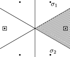
Figure 1. The root diagram of $\mathfrak{sl}(3,\mathbb{C})$

The parabolic subalgebra $\mathfrak{p}$ is associated with $\mathtt{E}=\mathtt{S}^{1}+\mathtt{S}^{2}$. Here $\{-\sigma_{1},-\sigma_{2}\}=\Delta(\mathfrak{k}^{\perp})\cap\Delta(\mathfrak{g}^{<0})$, and $\sigma_{1}+\sigma_{2}\in\Delta(\mathfrak{k})$ satisfies the condition of Theorem 1.1. Hence $D$ is pseudoconcave.

Example 3.9.

Let $D$ be the period domain with $h^{2,0}=2$ and $h^{1,1}=1$. Then $G_{\mathbb{R}}=SO(4,1)$, and the root diagram is depicted in Figure 2.

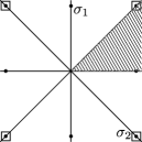
Figure 2. The root diagram of $\mathfrak{so}(5,\mathbb{C})$

The parabolic subalgebra $\mathfrak{p}$ is associated with $\mathtt{E}=\mathtt{S}^{1}$. Here $\{-\sigma_{1},-\sigma_{1}-\sigma_{2}\}=\Delta(\mathfrak{k}^{\perp})\cap\Delta(\mathfrak{g}^{<0})$, and $2\sigma_{1}+\sigma_{2}\in\Delta(\mathfrak{k})$ satisfies the condition. Hence $D$ is pseudoconcave.

4. Period domains

We review minimal degeneration for period domains and prove Theorem 4.4. Strategy of this proof is similar to the one of Theorem 1.1. We will show that a certain boundary point and an interior point are connected by a single cycle $gC_{0}$, which induces pseudoconcavity at the boundary orbit. We examine $sl_{2}$-triples associated with minimal degenerations for this proof.

In this section, $D$ is a period domain parametrizing Hodge structures of weight $n$ with Hodge numbers $\{h^{p,q}\}_{p+q=n}$ on a real vector space $V_{\mathbb{R}}$ polarized by $Q$. Here

$$G_{\mathbb{R}}=\mathop{\mathrm{Aut}}\nolimits{(V_{\mathbb{R}},Q)}\cong\begin{cases}Sp(m,\mathbb{R})&\text{if }n\text{ is odd,}\\ SO(m_{\mathrm{ev}},m_{\mathrm{od}})&\text{if }n\text{ is even}\end{cases}$$

where $2m=\mathop{\mathrm{dim}}\nolimits{V}$ if $n$ is odd, $m_{\mathrm{ev}}=\sum_{p\text{: even}}h^{p,q}$ and $m_{\mathrm{od}}=\sum_{p\text{: odd}}h^{p,q}$ if $n$ is even. We then have

$$D\cong\begin{cases}Sp(m,\mathbb{R})/\prod_{p<k}U(h^{p,q})&\text{if }n=2k+1,\\ SO(m_{\mathrm{ev}},m_{\mathrm{od}})/(\prod_{p<k}U(h^{p,q})\times SO(h^{k,k}))&\text{if }n=2k.\end{cases}$$

If we choose a reference point in $D$, then the $G_{\mathbb{R}}$-orbit $D$ is a flag domain contained in the $G$-orbit with $G=\mathop{\mathrm{Aut}}\nolimits{(V_{\mathbb{C}},Q)}$.

4.1. Nilpotent orbits and $SL_{2}$-orbits

We recall the nilpotent orbit theorem and the $SL_{2}$-orbit theorem of [S]. A pair $(N,F^{\bullet})$ consisting of a nilpotent $N\in\mathfrak{g}_{\mathbb{R}}$, as an element of $\mathop{\mathrm{End}}\nolimits{(V_{\mathbb{R}})}$, and $F^{\bullet}\in\check{D}$ is called a nilpotent orbit if it satisfies the following conditions:

• $\exp{(zN)}F^{\bullet}\in D$ if $\mathop{\mathrm{Im}}\nolimits{(z)}$ is sufficiently large;

• $NF^{p}\subset F^{p-1}.$

For a nilpotent orbit $(N,F^{\bullet})$, there exists the monodromy weight filtration $W_{\bullet}:=W_{\bullet}(N)[-n]$, and $(W_{\bullet},F^{\bullet})$ is a mixed Hodge structure, which is called the limit mixed Hodge structure.

Let $(N,F^{\bullet})$ be a nilpotent orbit such that $(W_{\bullet},F^{\bullet})$ is split over $\mathbb{R}$, i.e. the Deligne decomposition

$$V_{\mathbb{C}}=\bigoplus_{p,q}I^{p,q}$$

is defined over $\mathbb{R}$. We define $Y\in\mathfrak{g}_{\mathbb{R}}$ which acts on $I^{p,q}$ by the scalar $p+q-n$ and $N^{+}\in\mathfrak{g}_{\mathbb{R}}$ so that $(N^{+},Y,N)$ is a $sl_{2}$-triple in $\mathfrak{g}_{\mathbb{R}}$. The $SL_{2}$-orbit theorem guarantees existence of a homomorphism $v:SL(2,\mathbb{R})\to G_{\mathbb{R}}$ such that

$$v_{*}\begin{pmatrix}0&1\\ 0&0\end{pmatrix}=N^{+},\quad v_{*}\begin{pmatrix}1&0\\ 0&-1\end{pmatrix}=Y,\quad v_{*}\begin{pmatrix}0&0\\ 1&0\end{pmatrix}=N$$

and a $SL_{2}(\mathbb{C})$-equivalent horizontal holomorphic map $\psi:\mathbb{P}^{1}(\mathbb{C})\to\check{D}$ given by

$$\begin{pmatrix}1\\ z\end{pmatrix}\mapsto\exp{(zN)}F^{\bullet}$$

Here $\exp{(zN)}F^{\bullet}\in D$ for $\mathop{\mathrm{Im}}\nolimits{(z)}>0$, and $\psi$ defines a $SL_{2}(\mathbb{R})$-equivalent map from the upper half plane to $D$.

Let

$$\mathbf{d}_{N}:=\exp{(\mathbf{i}\frac{\pi}{4}(N^{+}+N))}.$$

We then have

$$\varphi:=\mathbf{d}_{N}(F^{\bullet})=\psi(\frac{1}{\sqrt{2}}\begin{pmatrix}1&\mathbf{i}\\ \mathbf{i}&1\end{pmatrix}\begin{pmatrix}1\\ 0\end{pmatrix})=\psi(\begin{pmatrix}1\\ \mathbf{i}\end{pmatrix})\in D,$$

which defines the Hodge decomposition

$$V_{\mathbb{C}}=\bigoplus V^{p,n-p}$$

and homomorphism $\varphi:S^{1}=\{z\in\mathbb{C}\;;\;|z|=1\}\to G_{\mathbb{R}}$ of real algebraic groups given by

$$\varphi(z)v=z^{2p-n}v\quad\text{for }v\in V^{p,n-p}.$$

The image $\varphi(S^{1})$ is contained in a compact maximal torus $T$ ([GGK1, Proposition IV.A.2]), and we define the Cartan subalgebra $\mathfrak{h}=\mathfrak{t}\otimes\mathbb{C}$. The associated grading element is $\mathtt{E}_{\varphi}=\frac{1}{4\pi\mathbf{i}}\varphi^{\prime}(1)\in\mathfrak{t}$, which satisfies

$$\mathtt{E}_{\varphi}v=\frac{2p-n}{2}v\quad\text{for }v\in V^{p,n-p}.$$

Now $\varphi$ defines a weight-$0$ real Hodge structure on $\mathfrak{g}$ with the polarization given by minus the Killing form $B$. Here the $(p,-p)$-component is the eigenspace

$$\mathfrak{g}^{p}=\{X\in\mathfrak{g}\;|\;\mathop{\mathrm{ad}}\nolimits{(\mathtt{E}_{\varphi})}X=pX\}=\{X\in\mathfrak{g}\;|\;XV^{k,n-k}\subset V^{k+p,n-k-p}\}.$$

The Lie algebra of the parabolic subgroup stabilizing $\varphi$ is $\mathfrak{p}=\bigoplus_{p\geq 0}\mathfrak{g}^{p}.$ Since $\varphi(\mathbf{i})$ is the Weil operator, $-B(\varphi(\mathbf{i})\bullet,\bullet)$ is positive definite. Therefore $\mathop{\mathrm{Ad}}\nolimits{(\varphi(\mathbf{i}))}$ is an Cartan involution defined over $\mathbb{R}$, which defines the Cartan decomposition $\mathfrak{g}_{\mathbb{R}}=\mathfrak{k}_{\mathbb{R}}\oplus\mathfrak{k}^{\perp}_{\mathbb{R}}$ such that

$$\mathfrak{k}_{\mathbb{R}}\otimes\mathbb{C}=\bigoplus_{p\text{: even}}\mathfrak{g}^{p},\quad\mathfrak{k}^{\perp}_{\mathbb{R}}\otimes\mathbb{C}=\bigoplus_{p\text{: odd}}\mathfrak{g}^{p}.$$

The maximal compact subalgebra $\mathfrak{k}_{\mathbb{R}}$ satisfies $\mathfrak{t}\subset\mathfrak{g}_{\mathbb{R}}\cap\mathfrak{p}\subset\mathfrak{k}_{\mathbb{R}}$, i.e. $D$ is measurable in the sense of [FHW, §4.5].

We set the $sl_{2}$-triple

$$(\bar{\mathcal{E}},\mathcal{Z},\mathcal{E}):=\mathop{\mathrm{Ad}}\nolimits_{\mathbf{d}_{N}}(N^{+},Y,N)$$

in $\mathfrak{g}_{\mathbb{C}}$. Then

$$\bar{\mathcal{E}}=\frac{1}{2}(N+N^{+}-\mathbf{i}Y),\quad\mathcal{Z}=\mathbf{i}(N-N^{+}),\quad\mathcal{E}=\frac{1}{2}(N+N^{+}+\mathbf{i}Y).$$

Since $NF^{p}\subset F^{p-1}$ by the property of nilpotent orbits, we have

$$\bar{\mathcal{E}}\in\mathfrak{g}^{1},\quad\mathcal{Z}\in\mathfrak{g}^{0},\quad\mathcal{E}\in\mathfrak{g}^{-1}.$$

Let $V_{\mathbb{C}}=\bigoplus V^{\mu}$ be the weight space decomposition with respect to $\mathfrak{h}$. That is, $\mu\in\mathfrak{h}^{*}$ and $v\in V^{\mu}$ if and only if $\xi(v)=\mu(\xi)v$ for all $\xi\in\mathfrak{h}$. Then we have $V^{p,n-p}=\bigoplus_{\mu(\mathtt{E}_{\varphi})=(2p-n)/2}V^{\mu}.$ The infinitesimal period relation is bracket-generating in the sense of [R, §3.12]. Then we have

(4.1) $$\mathbf{d}_{N}(I^{p,q})=\bigoplus_{\begin{subarray}{c}\mu(\mathtt{E}_{\varphi})=(2p-n)/2\\ \mu(\mathcal{Z})=p+q-n\end{subarray}}V^{\mu}=\{v\in V^{p,n-p}\;|\;\mathcal{Z}v=(p+q-n)v\}.$$

by [R, Theorem 5.5(d)] and [R, Theorem 5.9(b)].

4.2. Minimal degenerations

For a nilpotent orbit $(N,F^{\bullet})$, we have the reduced limit

$$F^{\bullet}_{\infty}=\lim_{\mathop{\mathrm{Im}}\nolimits{(z)}\to\infty}\exp{(zN)}F^{\bullet}\in\mathrm{bd}{(D)}.$$

A nilpotent orbit $(N,F^{\bullet})$ is called a minimal degeneration if $F^{\bullet}_{\infty}$ is in a real codimension-one boundary $G_{\mathbb{R}}$-orbit of $D$. Type of minimal degenerations is classified into two kinds as follows:

Theorem 4.1 ([GGR] Theorem 1.7).

A minimal degeneration in a period domain is either

• $N\neq 0$, $N^{2}=0$ and $\mathop{\mathrm{rank}}\nolimits{N}=1,2$, or

• $N^{2}\neq 0$, $N^{3}=0$ and $\mathop{\mathrm{rank}}\nolimits{N}=2$.

Moreover, type of minimal degeneration is determined by $\{i^{p,q}\}$, where $i^{p,q}=\mathop{\mathrm{dim}}\nolimits{I^{p,q}}$, and $\{h^{p,q}\}$ (see also Figure 3):

• $(N,F^{\bullet})$ is of type I if and only if there exists $p_{o}\in\mathbb{Z}$ such that $2p_{o}<n$ satisfying the following conditions:

  • $i^{p_{o}+1,n-p_{o}},i^{p_{o},n-p_{o}-1}=1$;

  • $i^{p_{o},n-p_{o}}=h^{p_{o},n-p_{o}}-1$ and $i^{p_{o}+1,n-p_{o}-1}=h^{p_{o}+1,n-p_{o}-1}-1$;

  • for all other $p$ such that $2p<n$, $i^{p,n-p}=h^{p,n-p}$.

• $(N,F^{\bullet})$ is of type II if and only if $n=2m$ is even and it satisfies the following conditions:

  • $i^{m-1,m-1},i^{m+1,m+1}=1$;

  • $i^{m-1,m+1}=h^{m-1,m+1}-1$ and $i^{m+1,m-1}=h^{m+1,m-1}-1$;

  • for all other $p$ such that $2p<n$, $i^{p,n-p}=h^{p,n-p}$.

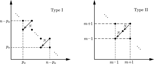
Figure 3. Deligne decompositions for minimal degenerations

Let $(N,F^{\bullet})$ be a minimal degeneration such that the limit mixed Hodge structure is $\mathbb{R}$-split. In this case, $N$ and $N^{+}$ are root vectors and $\mathbf{d}_{N}$ is the Cayley transform (see [GGK2, Appendix to Lecture 10] or [KP]).

Lemma 4.2.

(1) Suppose that $(N,F^{\bullet})$ is of type I. Let $v\in I^{p_{o}+1,n-p_{o}}$. We then have

$$\mathbf{d}_{N}(v)=\frac{1}{\sqrt{2}}(v+\mathbf{i}Nv), \mathbf{d}_{N}(Nv)=\frac{\mathbf{i}}{\sqrt{2}}(v-\mathbf{i}Nv),$$

$$\mathbf{d}_{N}(\bar{v})=\mathbf{i}\cdot\overline{\mathbf{d}_{N}(Nv)}, \mathbf{d}_{N}(N\bar{v})=\mathbf{i}\cdot\overline{\mathbf{d}_{N}(v)}.$$

In particular, if $n=2p_{o}+1$ and $v\in I^{p_{o}+1,p_{o}+1}\cap V_{\mathbb{R}}$, $\mathbf{d}_{N}(v)=\mathbf{i}\cdot\overline{\mathbf{d}_{N}(Nv)}$.

(2) Suppose that $(N,F^{\bullet})$ is of type II. Let $v\in I^{m+1,m+1}$. We then have

$$\mathbf{d}_{N}(v)=\frac{1}{2}v+\frac{1}{2}\mathbf{i}Nv-\frac{1}{4}N^{2}v,\quad\mathbf{d}_{N}(Nv)=\mathbf{i}(v+\frac{1}{2}N^{2}v),\quad\mathbf{d}_{N}(N^{2}v)=-2\overline{\mathbf{d}_{N}(v)}$$

Proof..

First, we prove (1). By property of limit mixed Hodge structure, $N$ is a $(-1,-1)$-endomorphism and the nil-positive element $N^{+}$ is a $(1,1)$-endomorphism of the limit mixed Hodge structure $(W_{\bullet},F^{\bullet})$. Moreover, $N$ is an isomorphism from $I^{p_{o}+1,n-p_{o}}$ to the image. Then

$$(N^{+}+N)v=Nv,\quad(N^{+}+N)^{2}v=N^{+}Nv=[N^{+},N]v=Yv=v.$$

and we have

$$\mathbf{d}_{N}(v)= \sum_{\ell=0}^{\infty}\frac{(-1)^{\ell}}{(2\ell)!}(\frac{\pi}{4})^{2\ell}v+\sum_{k=0}^{\infty}\frac{(-1)^{k}}{(2k+1)!}(\frac{\pi}{4})^{2k+1}\mathbf{i}Nv$$

$$=\cos{(\frac{\pi}{4})}v+\mathbf{i}\sin{(\frac{\pi}{4})}Nv=\frac{1}{\sqrt{2}}(v+\mathbf{i}Nv),$$

$$\mathbf{d}_{N}(Nv)= \sum_{\ell=0}^{\infty}\frac{(-1)^{\ell}}{(2\ell)!}(\frac{\pi}{4})^{2\ell}Nv+\sum_{k=0}^{\infty}\frac{(-1)^{k}}{(2k+1)!}(\frac{\pi}{4})^{2k+1}\mathbf{i}v$$

$$=\cos{(\frac{\pi}{4})}Nv+\mathbf{i}\sin{(\frac{\pi}{4})}v=\frac{\mathbf{i}}{\sqrt{2}}(v-\mathbf{i}Nv).$$

The equations for $\mathbf{d}_{N}(\bar{v})$ and $\mathbf{d}_{N}(N\bar{v})$ follows from similar calculations.

Next, we prove (2). By property of limit mixed Hodge structure,

$$N^{+}Nv=[N^{+},N]v=Yv=2v,$$

$$N^{+}N^{2}v=[N^{+},N]Nv+NN^{+}Nv=YNv+2Nv=2Nv.$$

(4.2) $$(N^{+}+N)v=Nv,\quad(N^{+}+N)^{2}v=N^{+}Nv+N^{2}v=2v+N^{2}v,$$

$$(N^{+}+N)^{3}v=2Nv+N^{+}N^{2}v=4Nv.$$

Then

$$\mathbf{d}_{N}(v)=v+\sum_{k=0}^{\infty}\frac{(-1)^{k}}{(2k+1)!}(\frac{\pi}{4})^{2k+1}4^{k}\mathbf{i}Nv+\sum_{\ell=1}^{\infty}\frac{(-1)^{\ell}}{(2\ell)!}(\frac{\pi}{4})^{2\ell}4^{\ell-1}(2v+N^{2}v).$$

Here

(4.3) $$\sum_{k=0}^{\infty}\frac{(-1)^{k}}{(2k+1)!}(\frac{\pi}{4})^{2k+1}4^{k}=\frac{1}{2}\sum_{k=0}^{\infty}\frac{(-1)^{k}}{(2k+1)!}(\frac{\pi}{4})^{2k+1}2^{2k+1}=\frac{1}{2}\sin{(\frac{\pi}{2})}=\frac{1}{2}$$

$$\sum_{\ell=1}^{\infty}\frac{(-1)^{\ell}}{(2\ell)!}(\frac{\pi}{4})^{2\ell}4^{\ell-1}=\frac{1}{4}\sum_{\ell=1}^{\infty}\frac{(-1)^{\ell}}{(2\ell)!}(\frac{\pi}{4})^{2\ell}2^{2\ell}=\frac{1}{4}(\cos{(\frac{\pi}{2})}-1)=-\frac{1}{4}.$$

Therefore,

$$\mathbf{d}_{N}(v)=\frac{1}{2}v+\frac{1}{2}\mathbf{i}Nv-\frac{1}{4}N^{2}v.$$

Since we have $(N^{+}+N)Nv=(N^{+}+N)^{2}v$, by using (4.2) and (4.3)

$$\mathbf{d}_{N}(Nv) =\sum_{\ell=0}^{\infty}\frac{(-1)^{\ell}}{(2\ell)!}(\frac{\pi}{4})^{2\ell}4^{\ell}(Nv)+\sum_{k=0}^{\infty}\frac{(-1)^{k}}{(2k+1)!}(\frac{\pi}{4})^{2k+1}4^{k}\mathbf{i}(2v+N^{2}v)$$

$$=\cos{(\frac{\pi}{2})}Nv+\frac{\mathbf{i}}{2}(2v+N^{2}v)=\mathbf{i}(v+\frac{1}{2}N^{2}v).$$

Since we have $(N^{+}+N)N^{2}v=N^{+}N^{2}v=2Nv$, by using (4.2) and (4.3)

$$\mathbf{d}_{N}(N^{2}v) =N^{2}v+\sum_{k=0}^{\infty}\frac{(-1)^{k}}{(2k+1)!}(\frac{\pi}{4})^{2k+1}4^{k}2\mathbf{i}Nv+\sum_{\ell=1}^{\infty}\frac{(-1)^{\ell}}{(2\ell)!}(\frac{\pi}{4})^{2\ell}4^{\ell-1}2(2v+N^{2}v)$$

$$=N^{2}v+\mathbf{i}Nv-\frac{1}{2}(2v+N^{2}v)=\frac{1}{2}N^{2}v+\mathbf{i}Nv-v=-2\overline{\mathbf{d}_{N}(v)}.$$

∎

4.3. Pseudoconcave boundary orbits

For a point in a codimension-one boundary orbit, we may define a local defining function. Considering its Levi form, we can define pseudoconcavity at a point in a codimension-one boundary orbit as Definition 2.1:

Definition 4.3.

A codimension-one boundary $G_{\mathbb{R}}$-orbit $\mathcal{O}$ in $\mathrm{bd}{(D)}$ is pseudoconcave boundary orbit of $D$ if a holomorphic map $\rho:\mathbb{D}\to\mathrm{c\ell}{(D)}$ where $\rho(0)\in\mathcal{O}$ and $\mathrm{bd}{(\rho(\mathbb{D}))}\subset D$ exists.

Let $\mathcal{O}$ be a codimension-one boundary $G_{\mathbb{R}}$-orbit. We have a minimal degeneration $(N,F^{\bullet})$ where the associated reduced limit $F^{\bullet}_{\infty}$ is in $\mathcal{O}$.

Theorem 4.4.

Suppose that there exists $r\in\mathbb{Z}$ such that $i^{r,n-r}\neq 0$ satisfying one of the following conditions:

1. $(N,F^{\bullet})$ is of type I and $r=p_{o}+2\ell$ or $r=p_{o}-2\ell+1$ ($\ell\geq 1$);

2. $(N,F^{\bullet})$ is of type II and $r=m+2\ell+1$ ($\ell\in\mathbb{Z}$).

Then $\mathcal{O}$ is a pseudoconcave boundary orbit of $D$.

Example 4.5.

Let $D$ be the period domain with $h^{3,0}=h^{2,1}=1$. This is the period domain for quintic-mirror threefolds. In this case, nontrivial nilpotent orbits and the Deligne–Hodge numbers of the limit mixed Hodge structures are classified into the following three types:

• $N^{2}=0$ and $\mathop{\mathrm{dim}}\nolimits{(\mathop{\mathrm{Im}}\nolimits{N})}=1$ ($i^{2,2}=i^{1,1}=i^{3,0}=i^{0,3}=1$);

• $N^{2}=0$ and $\mathop{\mathrm{dim}}\nolimits{(\mathop{\mathrm{Im}}\nolimits{N})}=2$ ($i^{3,1}=i^{1,3}=i^{2,0}=i^{0,2}=1$);

• $N^{3}\neq 0$ and $N^{4}=0$ ($i^{3,3}=i^{2,2}=i^{1,1}=i^{0,0}=1$).

Here (I) and (II) are minimal degeneration of type I. Moreover (I) satisfies the condition of Theorem 4.4, and then the corresponding codimension-one boundary $G_{\mathbb{R}}$-orbit is a pseudoconcave boundary orbit.

4.4. Proof of Theorem 4.4

For a nilpotent orbit $(N,F^{\bullet})$, there uniquely exists $\tilde{F}^{\bullet}\in\check{D}$ such that the limit mixed Hodge structure $(W_{\bullet},\tilde{F}^{\bullet})$ is $\mathbb{R}$-split by [CKS, Proposition 2.20]. Since $\mathcal{O}=G_{\mathbb{R}}F^{\bullet}_{\infty}=G_{\mathbb{R}}\tilde{F}^{\bullet}_{\infty}$ by [KP, §5.1], we may choose $F^{\bullet}\in\check{D}$ so that $F^{\bullet}=\tilde{F}^{\bullet}$.

We have $\varphi=\mathbf{d}_{N}(F^{\bullet})\in D$ as in §4.1. Let $K_{\mathbb{R}}$ be the maximal compact subgroup containing $G_{\mathbb{R}}\cap P$ where $P$ is the parabolic subgroup of $G$ stabilizing $\varphi$. We define the base cycle $C_{0}=K_{\mathbb{R}}\varphi$. For $\mathcal{E}=\mathop{\mathrm{Ad}}\nolimits_{\mathbf{d}_{N}}(N)$ we have

$$\exp{(\mathbf{i}\mathcal{E})}\varphi=\psi(\frac{1}{\sqrt{2}}\begin{pmatrix}1&\mathbf{i}\\ \mathbf{i}&1\end{pmatrix}\begin{pmatrix}1\\ \mathbf{i}\end{pmatrix})=F^{\bullet}_{\infty}.$$

By Lemma 4.6, $\exp{(\mathbf{i}\mathcal{E})}C_{0}\ni F^{\bullet}_{\infty}$ and $\exp{(\mathbf{i}\mathcal{E})}C_{0}\cap C_{0}\neq\emptyset$. We may construct $Z\subset gC_{0}$ and a disk $\mathbb{D}\subset Z$ about $F^{\bullet}_{\infty}$ satisfying $\mathrm{bd}{(\mathbb{D})}\subset D$ applying the discussion of the proof of [Huc1, Theorem 3.7].

Hence we prove Lemma 4.6, which completes the proof of Theorem 4.4.

Lemma 4.6.

If $r\in\mathbb{Z}$ satisfying the condition of Theorem 4.4 exists, then there exists $k\in K$ such that $\mathop{\mathrm{Ad}}\nolimits{(k)}(\mathcal{E})\in\mathfrak{p}$. In particular, $k^{-1}\varphi\in C_{0}$ is a fixed point of $\exp{(\lambda\mathcal{E})}$ with $\lambda\in\mathbb{C}$.

Proof..

We first consider the case for type I. Let $v\in I^{p_{o}+1,n-p_{o}}$. By Lemma 4.2

(4.4) $$\mathcal{E}\mathbf{d}_{N}(v)=\mathbf{d}_{N}(Nv),\quad\overline{\mathcal{E}\mathbf{d}_{N}(v)}=-\mathbf{i}\mathbf{d}_{N}(\bar{v}),$$

$$\mathcal{E}\cdot\overline{\mathcal{E}\mathbf{d}_{N}(v)}=-\mathbf{i}\mathbf{d}_{N}(N\bar{v})=\overline{\mathbf{d}_{N}(v)}.$$

In particular, if $n=2p_{o}+1$ and $v\in I^{p_{o}+1,p_{o}+1}\cap V_{\mathbb{R}}$, then

(4.5) $$\mathbf{d}_{N}(v)=\mathbf{i}\cdot\overline{\mathcal{E}\mathbf{d}_{N}(v)},\quad\mathcal{E}\cdot\overline{\mathcal{E}\mathbf{d}_{N}(v)}=-\mathbf{i}\mathcal{E}\mathbf{d}_{N}(v).$$

We put $w:=\mathcal{E}\mathbf{d}_{N}(v)$. We may assume $\|w\|=1$ for the Hodge norm $\|\bullet\|=Q(\varphi(\mathbf{i})\bullet,\bar{\bullet})$. Let $r=p_{o}+2\ell$ with $\ell\geq 1$ and $i^{r,n-r}\neq 0$. Since $I^{r,n-r}\subset W^{n}$ is contained in $\mathop{\mathrm{Ker}}\nolimits{N}$ by property of monodromy weight filtration, $I^{r,n-r}=\mathbf{d}_{N}(I^{r,n-r})\subset V^{r,n-r}$. We choose $u\in I^{r,n-r}$ so that $\|u\|=1$. We define $k\in\mathop{\mathrm{Aut}}\nolimits{(V_{\mathbb{C}})}$ by

(4.6) $$kw=u,\quad ku=w,\quad k\bar{u}=\bar{w},\quad k\bar{w}=\bar{u},$$

$$kv^{\prime}=v^{\prime}\quad\text{if }v^{\prime}\perp w,u,\bar{w}\text{ and }\bar{u}\text{ with respect to }Q.$$

Then $k\in G$, and $\mathop{\mathrm{Ad}}\nolimits{(\varphi(\mathbf{i}))}k=k$, i.e. $k\in K$ (see Figure 4).

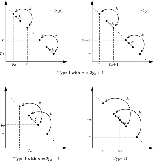
Figure 4. Hodge decompositions with respect to $\varphi$

By using (4.4) and (4.5) we have

$$\mathop{\mathrm{Ad}}\nolimits{(k)}(\mathcal{E})\mathbf{d}_{N}(v)=\begin{cases}\mathbf{i}\mathop{\mathrm{Ad}}\nolimits{(k)}(\mathcal{E})\bar{w}=\mathbf{i}k\mathcal{E}\bar{u}=0&\text{if }n=2p_{o}+1,\\ kw=u&\text{otherwise};\end{cases}$$

$$\mathop{\mathrm{Ad}}\nolimits{(k)}(\mathcal{E})\bar{u}=k\mathcal{E}\bar{w}=\begin{cases}-\mathbf{i}kw=-\mathbf{i}u&\text{if }n=2p_{o}+1,\\ \mathcal{E}\bar{w}=\overline{\mathbf{d}_{N}(v)}&\text{otherwise};\end{cases}$$

$$\mathop{\mathrm{Ad}}\nolimits{(k)}(\mathcal{E})v^{\prime}=0\quad\text{if }v^{\prime}\perp u\text{ and }\overline{\mathbf{d}_{N}(v)}.$$

Since $\mathbf{d}_{N}(v)\in V^{p_{o}+1,n-p_{o}-1}$ by (4.1), we conclude that

(4.7) $$\mathop{\mathrm{Ad}}\nolimits{(k)}\mathcal{E}\in\begin{cases}\mathfrak{g}^{4\ell-1}\subset\mathfrak{p}&\text{if }n=2p_{o}+1,\\ \mathfrak{g}^{2\ell-1}\subset\mathfrak{p}&\text{otherwise}.\end{cases}$$

For the case where $r=p_{o}-2\ell+1$ with $\ell\geq 1$, we put $w=\mathbf{d}_{N}(v)$ instead and define $k\in K$ as (4.6). Then we obtain (4.7).

Next, we consider the case for type II. Let $v\in I^{m+1,m+1}$ such that $\|\mathbf{d}_{N}(v)\|=1$ and put $w=\mathbf{d}_{N}(v)$. Then

$$\overline{\mathcal{E}w}=-\mathcal{E}w,\quad-2\bar{w}=\mathcal{E}^{2}w.$$

Let $r=m+2\ell+1$ with $i^{r,n-r}\neq 0$. Since $n-r=m+2(-\ell-1)+1$ and $i^{n-r,r}\neq 0$, we may assume $\ell<0$. We choose $u\in V^{r,n-r}$ so that $\|u\|=1$. We define $k\in K$ as (4.6), and then

$$\mathop{\mathrm{Ad}}\nolimits{(k)}(\mathcal{E})u=k\mathcal{E}w=\mathcal{E}w,\quad\mathop{\mathrm{Ad}}\nolimits{(k)}(\mathcal{E})\mathcal{E}w=-2\bar{u},$$

$$\mathop{\mathrm{Ad}}\nolimits{(k)}(\mathcal{E})v^{\prime}=0\quad\text{if }v^{\prime}\perp\bar{u}\text{ and }\overline{\mathcal{E}w}.$$

Since $\mathcal{E}w\in V^{m,m}$, we have $\mathop{\mathrm{Ad}}\nolimits{(k)}\mathcal{E}\in\mathfrak{g}^{-2\ell-1}\subset\mathfrak{p}$. ∎

References

- [A] A. Andreotti, Nine lectures on complex analysis. (Centro Internaz. Mat. Estivo C.I.M.E., I Ciclo, Bressanone, 1973), 1–175. Edizioni Cremonese, Rome, 1974.
- [C] H. Carayol, Cohomologie automorphe et compactifications partielles de certaines variétés de Griffiths-Schmid, Compos. Math. 141 (2005), no. 5, 1081–1102.
- [CG] J. Carlson and P. Griffiths, What is … a period domain?, Notices Amer. Math. Soc. 55 (2008), no. 11, 1418–-1419.
- [CKS] E. Cattani, A. Kaplan and W. Schmid, Degeneration of Hodge structures, Ann. of Math. 123 (1986), 457–535.
- [FHW] G. Fels, A. Huckleberry and J. A. Wolf, Cycle Spaces of Flag Domains: A Complex Geometric Viewpoint, Progress in Mathematics 45. Birkhäuser Boston, Inc., 2006.
- [GGK1] M. Green, P. Griffiths and M. Kerr, Mumford-Tate groups and domains: their geometry and arithmetic, Annals of Math Studies 183. Princeton University Press, 2012.
- [GGK2] M. Green, P. Griffiths and Matt Kerr,Hodge theory, complex geometry, and representation theory, CBMS Regional Conference Series in Mathematics 118. Published for the Conference Board of the Mathematical Sciences, Washington, DC, 2013.
- [GGR] M. Green, P. Griffiths and C. Robles, Extremal degenerations of polarized Hodge structures, preprint (arXiv:1403.0646).
- [GRT] P. Griffiths, C. Robles and D. Toledo, Quotients of non-classical flag domains are not algebraic, Algebr. Geom. 1 (2014), no. 1, 1–13.
- [Hum] J. Humphreys, Introduction to Lie algebras and representation theory, Graduate Texts in Mathematics, 9. Springer-Verlag, New York-Berlin, 1972.
- [Huc1] A. Huckleberry, Remarks on homogeneous manifolds satisfying Levi-conditions, Bollettino U.M.I. (9) III (2010) 1–23.
- [Huc2] A. Huckleberry, Hyperbolicity of cycle spaces and automorphism groups of flag domains, Amer. J. Math. 135 (2013), no. 2, 291–310.
- [Kn] A. Knapp, Lie groups beyond an introduction, second edition, Progress in Mathematics, 140. Birkhäuser Boston Inc., 2002.
- [Ko] J. Kollár, Neighborhoods of subvarieties in homogeneous spaces, Contemp. Math. 647 (2015), 91–108.
- [KP] M. Kerr and G. Pearlstein, Naive boundary strata and nilpotent orbits, Annales de l’Institut Fourier 64 (2014), no. 6, 2659–2714.
- [R] C. Robles, Classification of horizontal SL(2)’s, Compositio Math. 152 (2016), no. 05, 918–954.
- [S] W. Schmid, Variation of Hodge structure: the singularities of the period mapping, Invent. Math. 22 (1973), 211–319.