On conformal maps from multiply connected domains onto lemniscatic domains

Abstract

We study conformal maps from multiply connected domains in the extended complex plane onto lemniscatic domains. Walsh proved the existence of such maps in 1956 and thus obtained a direct generalization of the Riemann mapping theorem to multiply connected domains. For certain polynomial pre-images of simply connected sets we derive a construction principle for Walsh’s conformal map in terms of the Riemann map for the simply connected set. Moreover, we explicitly construct examples of Walsh’s conformal map for certain radial slit domains and circular domains.

Keywords conformal mapping; multiply connected domains; lemniscatic domains.

Mathematics Subject Classification (2010) 30C35; 30C20

1 Introduction

Let $\mathcal{K}$ be any simply connected domain (open and connected set) in the extended complex plane $\widehat{\mathbb{C}}$ with $\infty\in\mathcal{K}$ and with at least two boundary points. Then the Riemann mapping theorem guarantees the existence of a conformal map $\Phi$ from $\mathcal{K}$ onto the exterior of the unit disk, which is uniquely determined by the normalization conditions $\Phi(\infty)=\infty$ and $\Phi^{\prime}(\infty)>0$. The exterior of the unit disk therefore is considered the canonical domain every such domain $\mathcal{K}$ can be conformally identified with (in the Riemann sense). For domains $\mathcal{K}$ that are not simply connected the conformal identification with a suitable canonical domain is significantly more challenging. This fact has been well described already by Nehari in his classical monograph on conformal mappings from 1952 [31, Chapter 7], which identified five of the “more important” canonical slit domains (originally due to Koebe [23, p. 311]).

In recent years there has been a surge of interest in the theory and computation of conformal maps for multiply connected sets, which has been driven by the wealth of applications of conformal mapping techniques throughout the mathematical sciences. Many recent publications have dealt with canonical slit domains as those described by Nehari; see, e.g., [1, 5, 9, 12, 28, 29]. A related line of recent research in this context has focussed on the theory and computation of Schwarz-Christoffel mapping formulas from (the exterior of) finitely many non-intersecting disks (circular domains, see, e.g., [19]) onto (the exterior of) the same number of non-intersecting polygons; see, e.g., [3, 4, 7, 8, 10]. A review and comparison of both approaches is given in [11].

In this work we explore yet another idea which goes back to a paper of Walsh from 1956 [37]. Walsh’s canonical domain is a lemniscatic domain of the form

$$\mathcal{L}\mathrel{\mathop{:}}=\{w\in\widehat{\mathbb{C}}:|U(w)|>\mu\},\quad\text{where}\quad U(w)\mathrel{\mathop{:}}=\prod_{j=1}^{n}(w-a_{j})^{m_{j}},$$ (1)

$a_{1},\ldots,a_{n}\in\mathbb{C}$ are pairwise distinct, $m_{1},\ldots,m_{n}>0$ satisfy $\sum_{j=1}^{n}m_{j}=1$, and $\mu>0$. Note that the function $U$ in the definition of $\mathcal{L}$ is an analytic but in general multiple-valued function. Its absolute value is, however, single-valued. Walsh proved that if $\mathcal{K}$ is the exterior of $n\geq 1$ non-intersecting simply connected components, then $\mathcal{K}$ can be conformally identified with some lemniscatic domain $\mathcal{L}$ of the form (1); see Theorem 2.1 below for the complete statement. Walsh’s theorem is a direct generalization of the Riemann mapping theorem, and for $n=1$ the two results are in fact equivalent. Alternative proofs of Walsh’s theorem were given by Grunsky [15, 16] (see also [17, Theorem 3.8.3]), Jenkins [21] and Landau [24]. For some further remarks on Walsh’s theorem we refer to Gaier’s commentary in Walsh’s Selected Papers [39, pp. 374-377].

To our knowledge, apart from the different existence proofs, conformal maps related to Walsh’s lemniscatic domains, which we call lemniscatic maps, have rarely been studied. In particular, we are not aware of any example for lemniscatic maps in the previously published literature. In this work we derive a general construction principle for lemniscatic maps for polynomial pre-images of simply connected sets and we construct some explicit examples. We believe that our results are of interest not only from a theoretical but also from a practical point of view. Walsh’s lemniscatic map easily reveals the logarithmic capacity of $E=\widehat{\mathbb{C}}\backslash\mathcal{K}$ as well as the Green’s function with pole at infinity for $\mathcal{K}$, whose contour lines or level curves are important in polynomial approximation. Moreover, analogously to the construction of the classical Faber polynomials on compact and simply connected sets (cf. [6, 35]), lemniscatic maps allow to define generalized Faber polynomials on compact sets with several components; see [38]. While the classical Faber polynomials have found a wide range of applications in particular in numerical linear algebra (see, e.g., [2, 20, 26, 27, 34]) and more general numerical polynomial approximation (see, e.g., [13, 14]), the Faber–Walsh polynomials have not been used for similar purposes yet, as no explicit examples for lemniscatic maps have been known. In our follow-up paper [33] we present more details on the theory of Faber–Walsh polynomials as well as explicitly computed examples.

In Section 2 we state Walsh’s theorem, and discuss general properties of the conformal map onto lemniscatic domains. We then consider the explicit construction of lemniscatic maps: In Section 3 we derive a construction principle for the lemniscatic map for certain polynomial pre-images of simply connected compact sets. In Section 4 we construct the lemniscatic map for the exterior of two equal disks. Some brief concluding remarks in Section 5 close the paper.

2 General properties of the conformal map onto lemniscatic domains

Let us first consider a lemniscatic domain $\mathcal{L}$ as in (1). It is easy to see that its Green’s function with pole at infinity is given by

$$g_{\mathcal{L}}(w)=\log|U(w)|-\log(\mu).$$

Moreover,

$$c(\widehat{\mathbb{C}}\backslash\mathcal{L})\mathrel{\mathop{:}}=\lim_{w\rightarrow\infty}\,\exp(\log|w|-g_{\mathcal{L}}(w))=\mu$$

is the logarithmic capacity of $\widehat{\mathbb{C}}\backslash\mathcal{L}$. The following theorem on the conformal equivalence of lemniscatic domains and certain multiply connected domains is due to Walsh [37, Theorems 3 and 4].

Theorem 2.1.

Let $E\mathrel{\mathop{:}}=\cup_{j=1}^{n}E_{j}$, where $E_{1},\ldots,E_{n}\subseteq\mathbb{C}$ are mutually exterior simply connected compact sets (none a single point) and let $\mathcal{K}\mathrel{\mathop{:}}=\widehat{\mathbb{C}}\backslash E$. Then there exist a unique lemniscatic domain $\mathcal{L}$ of the form (1) and a unique bijective conformal map

$$\Phi:\mathcal{K}\to\mathcal{L}\quad\mbox{with}\quad\Phi(z)=z+\mathcal{O}\left(\frac{1}{z}\right)\quad\text{for $z$ near infinity}.$$ (2)

In particular,

$$g_{\mathcal{K}}(z)=g_{\mathcal{L}}(\Phi(z))=\log|U(\Phi(z))|-\log(\mu)$$ (3)

is the Green’s function with pole at infinity of $\mathcal{K}$, and the logarithmic capacity of $E$ is $c(E)=c(\widehat{\mathbb{C}}\backslash\mathcal{L})=\mu$. The function $\Phi$ is called the lemniscatic map of $\mathcal{K}$ (or of $E$).

Note that for $n=1$ the lemniscatic domain $\mathcal{L}$ is the exterior of a disk with radius $\mu>0$, and Theorem 2.1 is equivalent to the classical Riemann mapping theorem.

If, for the given set $\mathcal{K}$, the function $\widetilde{\Phi}:\mathcal{K}\to\widetilde{\mathcal{L}}$ is any conformal map onto a lemniscatic domain that is normalized by $\widetilde{\Phi}(\infty)=\infty$ and $\widetilde{\Phi}^{\prime}(\infty)=1$, then $\widetilde{\Phi}(z)=\Phi(z)+b$ with $\Phi$ from Theorem 2.1 and some $b\in\mathbb{C}$. This uniqueness up to translation of lemniscatic domains follows from a more general theorem of Walsh [37, Theorem 4] by taking into account the normalization of $\widetilde{\Phi}$. This fact has already been noted by Motzkin in his MathSciNet review of [38].

Let $\sigma>1$, and let

$$\Gamma_{\sigma}=\{z\in\mathcal{K}:g_{\mathcal{K}}(z)=\log(\sigma)\}\quad\mbox{and}\quad\Lambda_{\sigma}=\{w\in\mathcal{L}:g_{\mathcal{L}}(w)=\log(\sigma)\}$$

be the level curves of $g_{\mathcal{K}}$ and $g_{\mathcal{L}}$, respectively. Then (3) implies $\Phi(\Gamma_{\sigma})=\Lambda_{\sigma}$, and thus

$$\Phi:\operatorname{ext}(\Gamma_{\sigma})\to\operatorname{ext}(\Lambda_{\sigma})=\{w\in\widehat{\mathbb{C}}:|U(w)|>\sigma\mu\}$$

is the lemniscatic map of the exterior of $\Gamma_{\sigma}$, provided that $\Gamma_{\sigma}$ still has $n$ components. (This holds exactly when the zeros of $g_{\mathcal{K}}^{\prime}$ lie exterior to $\Gamma_{\sigma}$.) Thus, we may “thicken” the given set $E=\widehat{\mathbb{C}}\backslash\mathcal{K}$, and $\Phi$ still is the corresponding lemniscatic map. An illustration is given in Figure 1 for a compact set composed of three radial slits from Corollary 3.3 below (with parameters $n=3$, $C=1$ and $D=2$) and for $\Gamma_{\sigma}$ with $\sigma=1.15$.

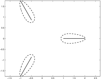
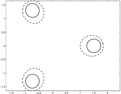
Figure 1: Left: The set $E$ consisting of three radial slits (solid) and the “thickened” set bounded by $\Gamma_{\sigma}$ for $\sigma=1.15$ (dashed). Right: The corresponding lemniscatic domains.

The next result shows that certain symmetry properties of the domain $\mathcal{K}$ imply corresponding properties of its lemniscatic map $\Phi$ and the lemniscatic domain $\mathcal{L}$. Here we consider rotational symmetry as well as symmetry with respect to the real and the imaginary axis.

Lemma 2.2.

In the notation of Theorem 2.1 we have:

1. If $\mathcal{K}=e^{i\theta}\mathcal{K}\mathrel{\mathop{:}}=\{e^{i\theta}z:z\in\mathcal{K}\}$, then $\Phi(z)=e^{-i\theta}\Phi(e^{i\theta}z)$ and $\mathcal{L}=e^{i\theta}\mathcal{L}$.

2. If $\mathcal{K}=\mathcal{K}^{\ast}\mathrel{\mathop{:}}=\{\overline{z}:z\in\mathcal{K}\}$, then $\Phi(z)=\overline{\Phi(\overline{z})}$ and $\mathcal{L}=\mathcal{L}^{*}$.

3. If $\mathcal{K}=-\mathcal{K}^{*}$, then $\Phi(z)=-\overline{\Phi(-\overline{z})}$ and $\mathcal{L}=-\mathcal{L}^{*}$.

In each case $\Phi^{-1}$ has the same symmetry property as $\Phi$.

Proof.

We only prove the first assertion; the proofs of the others are similar. Define the function $\widetilde{\Phi}$ on $\mathcal{K}$ by $\widetilde{\Phi}(z)\mathrel{\mathop{:}}=e^{-i\theta}\Phi(e^{i\theta}z)$. Then

$$\widetilde{\Phi}(\mathcal{K})=e^{-i\theta}\Phi(e^{i\theta}\mathcal{K})=e^{-i\theta}\Phi(\mathcal{K})=e^{-i\theta}\mathcal{L},$$

and $\widetilde{\Phi}:\mathcal{K}\to e^{-i\theta}\mathcal{L}$ is a bijective conformal map onto a lemniscatic domain with a normalization as in (2). Since the lemniscatic map of $\mathcal{K}$ is unique, we have $\Phi(z)=\widetilde{\Phi}(z)=e^{-i\theta}\Phi(e^{i\theta}z)$ and $\mathcal{L}=e^{-i\theta}\mathcal{L}$, or equivalently $\mathcal{L}=e^{i\theta}\mathcal{L}$.

Suppose that $\Phi(z)=e^{-i\theta}\Phi(e^{i\theta}z)$ for all $z\in\mathcal{K}$. Writing $w=\Phi(z)$ we get

$$\Phi^{-1}(e^{i\theta}w)=\Phi^{-1}(e^{i\theta}\Phi(z))=\Phi^{-1}(\Phi(e^{i\theta}z))=e^{i\theta}z=e^{i\theta}\Phi^{-1}(w),$$

which completes the proof. ∎

Finally, we show how a linear transformation of the set affects the lemniscatic map.

Lemma 2.3.

In the notation of Theorem 2.1, consider a linear transformation $\tau(w)=aw+b$ with $a\neq 0$, then

$$\tau(\mathcal{L})=\Big{\{}\widetilde{w}\in\widehat{\mathbb{C}}:\prod_{j=1}^{n}|\widetilde{w}-\tau(a_{j})|^{m_{j}}>|a|\mu\Big{\}}$$

is a lemniscatic domain and $\widetilde{\Phi}\mathrel{\mathop{:}}=\tau\circ\Phi\circ\tau^{-1}$ is the lemniscatic map of $\tau(\mathcal{K})$.

Proof.

With $\widetilde{w}=\tau(w)=aw+b$ we have

$$\prod_{j=1}^{n}|\widetilde{w}-\tau(a_{j})|^{m_{j}}=\prod_{j=1}^{n}|aw-aa_{j}|^{m_{j}}=|a|\prod_{j=1}^{n}|w-a_{j}|^{m_{j}},$$

and hence $\tau(\mathcal{L})$ is a lemniscatic domain. Clearly, $\widetilde{\Phi}:\tau(\mathcal{K})\to\tau(\mathcal{L})$ is a bijective and conformal map with Laurent series at infinity

$$\widetilde{\Phi}(z)=a\Phi\Big{(}\frac{z-b}{a}\Big{)}+b=z+\mathcal{O}\left(\frac{1}{z}\right).$$

Thus, $\widetilde{\Phi}$ is the lemniscatic map of $\tau(\mathcal{K})$. ∎

Lemma 2.3 can be applied to the lemniscatic maps we will derive in Sections 3 and 4 in order to obtain lemniscatic maps for further sets.

3 Lemniscatic maps and polynomial pre-images

In this section we discuss the construction of lemniscatic maps if the set $E$ is a polynomial pre-image of a simply connected compact set $\Omega$. We first exhibit the intricate relation between the lemniscatic map for $E$ and the exterior Riemann map for $\Omega$ in the general case. Under some additional assumptions we obtain an explicit formula for the lemniscatic map in terms of the Riemann map; see Theorem 3.1 below.

Let $\Omega\subseteq\mathbb{C}$ be a compact and simply connected set (not a single point) and let

$$\widetilde{\Phi}:\widehat{\mathbb{C}}\backslash\Omega\rightarrow\{w\in\widehat{\mathbb{C}}:|w|>1\}\quad\text{with}\quad\widetilde{\Phi}(\infty)=\infty,\quad\widetilde{\Phi}^{\prime}(\infty)>0,$$ (4)

be the exterior Riemann map of $\Omega$. Suppose that

$$E\mathrel{\mathop{:}}=P^{-1}(\Omega)$$

consists of $n\geq 2$ simply connected compact components (none a single point), where $P(z)=\alpha_{d}z^{d}+\alpha_{d-1}z^{d-1}+\ldots+\alpha_{0}$ is a polynomial with $\alpha_{d}\neq 0$. As above, let $\mathcal{K}\mathrel{\mathop{:}}=\widehat{\mathbb{C}}\backslash E$ and let

$$\Phi:\mathcal{K}\to\mathcal{L}=\{w\in\widehat{\mathbb{C}}:|U(w)|>\mu\}$$

be the lemniscatic map of $\mathcal{K}$. Then the Green’s function with pole at infinity for $\mathcal{K}$ is given by (3), and can also be expressed as

$$g_{\mathcal{K}}(z)=\log|U(\Phi(z))|-\log(\mu)=\frac{1}{d}g_{\widehat{\mathbb{C}}\backslash\Omega}(P(z))=\frac{1}{d}\log|\widetilde{\Phi}(P(z))|;$$

see the proof of Theorem 5.2.5 in [32]. This shows that $\Phi$ and $\widetilde{\Phi}$ are related by

$$|U(\Phi(z))|=\mu|\widetilde{\Phi}(P(z))|^{1/d},$$ (5)

where

$$\mu=c(E)=\left(\frac{c(\Omega)}{|\alpha_{d}|}\right)^{1/d}=\left(\frac{1}{|\alpha_{d}|\widetilde{\Phi}^{\prime}(\infty)}\right)^{1/d};$$

see [32, Theorem 5.2.5]. If $\widetilde{\Phi}$ and $P$ are known, the equality (5) yields a formula for (the modulus of) $U\circ\Phi$. However, this does not lead to separate expressions for $U$ and $\Phi$. In other words, we can in general neither obtain the lemniscatic domain nor the lemniscatic map directly via (5) from the knowledge of $\widetilde{\Phi}$ and $P$.

For certain sets $\Omega$ and polynomials $P$, we obtain by a direct construction explicit formulas for $U$ and $\Phi$ in terms of the Riemann map $\widetilde{\Phi}$.

Theorem 3.1.

Let $\Omega=\Omega^{*}\subseteq\mathbb{C}$ be compact and simply connected (not a single point) with exterior Riemann map $\widetilde{\Phi}$ as in (4). Let $P(z)=\alpha z^{n}+\alpha_{0}$ with $n\geq 2$, $\alpha_{0}\in\mathbb{R}$ to the left of $\Omega$, and $\alpha>0$.

Then $E\mathrel{\mathop{:}}=P^{-1}(\Omega)$ is the disjoint union of $n$ simply connected compact sets, and

$$\Phi:\widehat{\mathbb{C}}\backslash E\to\mathcal{L}=\{w\in\widehat{\mathbb{C}}:|U(w)|>\mu\},$$ (6)

$$\Phi(z)=z\Big{(}\frac{\mu^{n}}{z^{n}}[(\widetilde{\Phi}\circ P)(z)-(\widetilde{\Phi}\circ P)(0)]\Big{)}^{\frac{1}{n}},$$ (7)

is the lemniscatic map of $E$, where we take the principal branch of the $n$th root, and where

$$\mu\mathrel{\mathop{:}}=\Big{(}\frac{1}{\alpha\widetilde{\Phi}^{\prime}(\infty)}\Big{)}^{\frac{1}{n}}>0,\quad\text{and}\quad U(w)\mathrel{\mathop{:}}=(w^{n}+\mu^{n}(\widetilde{\Phi}\circ P)(0))^{\frac{1}{n}}.$$ (8)

Proof.

We construct the lemniscatic map $\Phi$ first in the sector

$$S=\Big{\{}z\in\mathbb{C}\backslash\{0\}:-\frac{\pi}{n}<\arg(z)<\frac{\pi}{n}\Big{\}},$$

and then extend it by the Schwarz reflection principle.

Since $z\in E$ if and only if $z^{n}\in\frac{1}{\alpha}(\Omega-\alpha_{0})$, the set $E$ has a single component $E_{1}$ in the sector $S$, obtained by taking the principal branch of the $n$th root. Note that $E_{1}=E_{1}^{*}\subseteq S$ is again a simply connected compact set. Then $E=\cup_{j=1}^{n}e^{i2\pi j/n}E_{1}$ is the disjoint union of $n$ simply connected compact sets.

Starting in $S\backslash E_{1}$, we construct the lemniscatic map as a composition of bijective conformal maps, see Figure 2:

1. The function $z_{1}=P(z)$ maps $S\backslash E_{1}$ onto the complement of $]-\infty,\alpha_{0}]\cup\Omega$.

2. Then $z_{2}=\widetilde{\Phi}(z_{1})$ maps this domain onto the complement of $]-\infty,\widetilde{\Phi}(\alpha_{0})]\cup\{z_{2}:|z_{2}|\leq 1\}$. Note that $\Omega=\Omega^{*}$ implies that $\widetilde{\Phi}(z)=\overline{\widetilde{\Phi}(\overline{z})}$, so that $]-\infty,\alpha_{0}]$ is mapped to the real line. In particular, $\widetilde{\Phi}(\alpha_{0})<-1$.

3. The function $z_{3}=\mu^{n}(z_{2}-\widetilde{\Phi}(\alpha_{0}))$ maps the previous domain onto the complement of $]-\infty,0]\cup\{z_{3}\in\mathbb{C}:|z_{3}+\mu^{n}\widetilde{\Phi}(\alpha_{0})|\leq\mu^{n}\}$. Here $\mu>0$ is defined by (8).

4. Finally, $w=z_{3}^{1/n}$, where we take the principal branch of the square root, maps this domain onto $S\cap\{w:|w^{n}+\mu^{n}\widetilde{\Phi}(\alpha_{0})|>\mu^{n}\}$.

(a) $z$-plane

(b) $z_{1}=P(z)$

(c) $z_{3}=\mu^{n}(\widetilde{\Phi}(z_{1})-\widetilde{\Phi}(\alpha_{0}))$

(d) $w=z_{3}^{1/n}$

Figure 2: Construction of the lemniscatic map in the proof of Theorem 3.1.

Since each map is bijective and conformal, their composition $\Phi$ is a bijective conformal map from $S\backslash E_{1}$ to $S\cap\{w\in\widehat{\mathbb{C}}:|U(w)|>\mu\}$. A short computation shows that

$$\Phi(z)=(\mu^{n}[(\widetilde{\Phi}\circ P)(z)-(\widetilde{\Phi}\circ P)(0)])^{\frac{1}{n}}=z\Big{(}\frac{\mu^{n}}{z^{n}}[(\widetilde{\Phi}\circ P)(z)-(\widetilde{\Phi}\circ P)(0)]\Big{)}^{\frac{1}{n}}$$

for $z\in S\backslash E_{1}$. Since $\Phi$ maps the half-lines $\arg(z)=\pm\frac{\pi}{n}$ onto themselves, $\Phi$ can be extended by Schwarz’ reflection principle to a bijective and conformal map from $(\widehat{\mathbb{C}}\backslash E)\backslash\{0,\infty\}$ to $\mathcal{L}\backslash\{0,\infty\}$. Note that $\Phi$ is given by (7) for every $z\in(\widehat{\mathbb{C}}\backslash E)\backslash\{0,\infty\}$, since the right hand side of (7) is analytic there. This follows since the expression under the $n$th root lies in $\mathbb{C}\backslash]-\infty,0]$ for every $z\in(\widehat{\mathbb{C}}\backslash E)\backslash\{0,\infty\}$.

It remains to show that $\Phi$ is defined and conformal in $0$ and $\infty$, and that it satisfies the normalization in (2). We begin with the point $z=0$. Near $\alpha_{0}$ the Riemann mapping $\widetilde{\Phi}$ has the form

$$\widetilde{\Phi}(z)=\widetilde{\Phi}(\alpha_{0})+\widetilde{\Phi}^{\prime}(\alpha_{0})(z-\alpha_{0})+\mathcal{O}((z-\alpha_{0})^{2}).$$

Then near $0$ we have

$$\Phi(z)=z\Big{(}\frac{\mu^{n}}{z^{n}}[\widetilde{\Phi}^{\prime}(\alpha_{0})\alpha z^{n}+\mathcal{O}(z^{2n})]\Big{)}^{\frac{1}{n}}=z\Big{(}\mu^{n}\widetilde{\Phi}^{\prime}(\alpha_{0})\alpha+\mathcal{O}(z^{n})\Big{)}^{\frac{1}{n}},$$

so that $\Phi(0)=0$, and $\Phi^{\prime}(0)=(\mu^{n}\widetilde{\Phi}^{\prime}(\alpha_{0})\alpha)^{\frac{1}{n}}\neq 0$, showing that $\Phi$ is defined and conformal at $0$.

Near $z=\infty$, we have $\widetilde{\Phi}(z)=\widetilde{\Phi}^{\prime}(\infty)z+\mathcal{O}(1)$, so that, together with (8),

$$\Phi(z)=z\Big{(}\frac{\mu^{n}}{z^{n}}[\widetilde{\Phi}^{\prime}(\infty)\alpha z^{n}+\mathcal{O}(1)]\Big{)}^{\frac{1}{n}}=z\Big{(}1+\mathcal{O}\Big{(}\frac{1}{z^{n}}\Big{)}\Big{)}^{\frac{1}{n}}=z+\mathcal{O}\Big{(}\frac{1}{z^{n-1}}\Big{)}.$$

Thus $\Phi$ satisfies (2) and is a bijective conformal map from $\widehat{\mathbb{C}}\backslash E$ to $\mathcal{L}$, as claimed. ∎

The assumption $\alpha>0$ in Theorem 3.1 has been made for simplicity only. In the notation of the theorem, if $P_{\theta}(z)=\alpha e^{i\theta}z^{n}+\alpha_{0}$ with $\theta\in\mathbb{R}$, then $P_{\theta}(z)=P(e^{i\theta/n}z)$. Hence $P_{\theta}^{-1}(\Omega)=e^{-i\theta/n}E=\tau(E)$, with $\tau(z)=e^{-i\theta/n}z$. Then the lemniscatic map of $\widehat{\mathbb{C}}\backslash P_{\theta}^{-1}(\Omega)$ is $\tau\circ\Phi\circ\tau^{-1}$; see Lemma 2.3.

Also note that if $\Omega$ is symmetric with respect to the line through the origin and some point $e^{i\theta}$, then, taking $\alpha_{0}$ on that line to the left of $\Omega$, the assertion of Theorem 3.1 remains unchanged.

Example 3.2.

As an example we consider the compact set $\Omega$ in Figure 3(b), which is of the form introduced in [22, Theorem 3.1]. It is defined with the parameters $\lambda=-1$, $\phi=\frac{\pi}{2}$ and $R=1.1$ through the inverse of its Riemann map

$$\widetilde{\Phi}^{-1}(w)=\frac{(w-\lambda N)(w-\lambda M)}{(N-M)w+\lambda(MN-1)},$$

where

$$Q=\tan(\phi/4)+\frac{1}{\cos(\phi/4)},\quad N=\frac{1}{2}\left(\frac{Q}{R}+\frac{R}{Q}\right),\quad M=\frac{R^{2}-1}{2R\tan(\phi/4)}.$$

Then $\Omega$ is the compact set bounded by $\widetilde{\Phi}^{-1}(\{w\in\mathbb{C}:|w|=1\})$, and thus has, in particular, an analytic boundary. Since $\Omega=\Omega^{*}$ and $\alpha_{0}=0$ lies to the left of $\Omega$, we can apply Theorem 3.1 with $P(z)=z^{3}$. Figure 3(a) shows the set $E=P^{-1}(\Omega)$, and Figure 3(c) shows the corresponding lemniscatic domain.

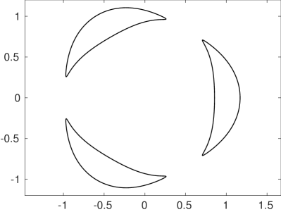
(a) $E=P^{-1}(\Omega)$ with $P(z)=z^{3}$

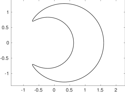
(b) Compact set $\Omega=\Omega^{*}$.

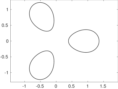
(c) Lemniscatic domain $\mathcal{L}$

Figure 3: Illustration of Theorem 3.1 with a set from [22, Theorem 3.1].

Using Theorem 3.1 we now derive the lemniscatic conformal map for a radial slit domain.

Corollary 3.3.

Let $E=\cup_{j=1}^{n}e^{i2\pi j/n}[C,D]$ with $0<C<D$. Then

$$\Phi(z)=z\Big{(}\frac{1}{2}+\frac{\sqrt{D}^{n}\sqrt{C}^{n}}{2}\frac{1}{z^{n}}\pm\frac{1}{2z^{n}}\sqrt{(z^{n}-C^{n})(z^{n}-D^{n})}\Big{)}^{\frac{1}{n}}$$ (9)

is the lemniscatic map of $E$ with corresponding lemniscatic domain

$$\mathcal{L}=\left\{w\in\widehat{\mathbb{C}}:|U(w)|=\left\lvert w^{n}-\frac{(\sqrt{D}^{n}+\sqrt{C}^{n})^{2}}{4}\right\rvert^{\frac{1}{n}}>\mu=\Big{(}\frac{D^{n}-C^{n}}{4}\Big{)}^{\frac{1}{n}}\right\}.$$ (10)

The inverse of $\Phi$ is given by

$$\Phi^{-1}(w)=w\left(1+\frac{(\sqrt{D}^{n}-\sqrt{C}^{n})^{2}}{4}\frac{1}{w^{n}-\frac{(\sqrt{D}^{n}+\sqrt{C}^{n})^{2}}{4}}\right)^{\frac{1}{n}},$$ (11)

where we take the principal branch of the $n$th root.

Proof.

With $P(z)=z^{n}$ and $\Omega=[C^{n},D^{n}]$ we have $E=P^{-1}(\Omega)$, and Theorem 3.1 applies. We need the conformal map

$$\widetilde{\Phi}:\widehat{\mathbb{C}}\backslash[C^{n},D^{n}]\to\{w\in\widehat{\mathbb{C}}:|w|>1\},\quad\widetilde{\Phi}(\infty)=\infty,\quad\widetilde{\Phi}^{\prime}(\infty)>0.$$

Clearly, its inverse is given by

$$\widetilde{\Phi}^{-1}(w)=\frac{D^{n}-C^{n}}{4}\Big{(}w+\frac{1}{w}\Big{)}+\frac{D^{n}+C^{n}}{2},$$

so that

$$\widetilde{\Phi}(z)=\frac{2}{D^{n}-C^{n}}\Big{(}z-\frac{D^{n}+C^{n}}{2}\pm\sqrt{(z-C^{n})(z-D^{n})}\Big{)},$$

where the branch of the square root is chosen such that $|\widetilde{\Phi}(z)|>1$. In particular, $\widetilde{\Phi}^{\prime}(\infty)=\frac{4}{D^{n}-C^{n}}$. Using this in Theorem 3.1 yields (9) and (10). By reversing the construction in the proof of Theorem 3.1, we see that

$$\Phi^{-1}(w)=\Big{(}\widetilde{\Phi}^{-1}\Big{(}\frac{w^{n}}{\mu^{n}}+\widetilde{\Phi}(0)\Big{)}\Big{)}^{\frac{1}{n}},$$

which, after a short computation, yields (11). ∎

Corollary 3.3 shows, in particular, that $\left(\frac{D^{n}-C^{n}}{4}\right)^{1/n}$ is the logarithmic capacity of $E=\cup_{j=1}^{n}e^{i2\pi j/n}[C,D]$; see [18].

Let us have a closer look at Corollary 3.3 in the case $n=2$, i.e.,

$$E=[-D,-C]\cup[C,D].$$

First note that in this case Corollary 3.3 gives a new proof for the well-known fact that the logarithmic capacity of $E$ is $c(E)=\tfrac{\sqrt{D^{2}-C^{2}}}{2}$; see, e.g., [32, Corollary 5.2.6] and [18]. Figure 4 shows phase portraits of $\Phi$ and $\psi\mathrel{\mathop{:}}=\Phi^{-1}$ for the values $C=0.1$ and $D=1$; see [40, 41] for details on phase portraits. The black lines in the left figure are the two intervals forming $E$, and the black curves in the right figure are the boundary of $\mathcal{L}$. At the black and white dots the functions have the values $0$ and $\infty$, respectively. The zeros of $\psi$ are $0$ and $\pm\sqrt{DC}$. The function $\psi:\mathcal{L}\to\mathcal{K}$ can be continued analytically (but not conformally) to a full neighbourhood of the lemniscate $\{w:|w^{2}-\frac{(D+C)^{2}}{4}|=\frac{D^{2}-C^{2}}{4}\}$. The zeros of $\psi^{\prime}$ are denoted by black crosses. Note the discontinuity of the phase of $\psi$ between the zeros and singularities interior to the lemniscate. This suggests that $\psi$ will be analytic and single-valued in $\{w\in\widehat{\mathbb{C}}:|U(w)|>\tfrac{D-C}{2}\}$.

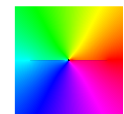
(a) Phase portrait of $\Phi$.

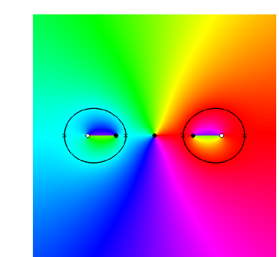
(b) Phase portrait of $\Phi^{-1}$.

Figure 4: Phase portraits of $\Phi$ and $\Phi^{-1}$ from Corollary 3.3 for $n=2$ and $C=0.1$ and $D=1$.

4 Lemniscatic map for two equal disks

In this section we analytically construct the lemniscatic map of a set $E$ that is the union of two disjoint equal disks. Let us denote by $D_{r}(z_{0})=\{z\in\mathbb{C}:|z-z_{0}|\leq r\}$ the closed disk with radius $r>0$ and center $z_{0}\in\mathbb{C}$. By Lemma 2.3 we can assume without loss of generality that $E=D_{r}(z_{0})\cup D_{r}(-z_{0})$ with real $z_{0}$ and $0<r<z_{0}$. Let $P(z)=\alpha z^{2}+\alpha_{0}$ with $\alpha>0$, then

$$\Omega=\{\alpha(z_{0}+\rho e^{it})^{2}+\alpha_{0}:0\leq\rho\leq r,0\leq t\leq 2\pi\}$$

is a simply connected compact set with $E=P^{-1}(\Omega)$, so that in principle we could apply Theorem 3.1. However, the Riemann map for the set $\Omega$ seems not to be readily available. Therefore, we directly construct the lemniscatic map as a composition of certain conformal maps. The main ingredients are the map from the exterior of two disks onto the exterior of two intervals and from there onto a lemniscatic domain (according to Corollary 3.3).

We need the following conformal map from [31, pp. 293–295].

Lemma 4.1.

Let $0<\rho<1$ and define

$$L=L(\rho)\mathrel{\mathop{:}}=2\rho\prod_{n=1}^{\infty}\Big{(}\frac{1+\rho^{8n}}{1+\rho^{8n-4}}\Big{)}^{2},$$ (12)

and the complete elliptic integral of the first kind

$$K=K(k)\mathrel{\mathop{:}}=\int_{0}^{1}\frac{dt}{\sqrt{(1-t^{2})(1-k^{2}t^{2})}}\quad\text{with }k\mathrel{\mathop{:}}=L^{2}.$$ (13)

Then the function

$$w=f(z)=L\operatorname{sn}\Big{(}\frac{2K}{\pi}i\log\Big{(}\frac{z}{\rho}\Big{)}+K;k\Big{)}$$ (14)

is a bijective and conformal map from the annulus $\rho<|z|<\rho^{-1}$ onto the $w$-plane with the slits $-\infty<w\leq-\tfrac{1}{L}$, $-L\leq w\leq L$ and $\tfrac{1}{L}\leq w<\infty$. Further, we have $f(-1)=-1$ and $f^{\prime}(-1)=(1-L^{2})\tfrac{2K}{\pi}>0$, and $f(z^{-1})=(f(z))^{-1}$.

Proof.

See [31, pp. 293–295] for the existence and mapping properties of $f$. Note that $f$ is independent of the choice of the branch of the logarithm. By construction $f$ is also symmetric with respect to the real axis and to the unit circle, i.e., $f(z)=\overline{f(\overline{z})}$, and $f(z)=1/\overline{f(1/\overline{z})}$. This implies $f(1/z)=1/\overline{f(\overline{z})}=1/f(z)$.

It remains to compute $f(-1)$ and $f^{\prime}(-1)$. Recall the identity

$$\operatorname{sn}^{\prime}(z;k)=\operatorname{cn}(z;k)\operatorname{dn}(z;k),$$

where $\operatorname{cn}(z;k)=\sqrt{1-\operatorname{sn}(z;k)^{2}}$, $\operatorname{cn}(0)=1$, and $\operatorname{dn}(z)=\sqrt{1-k^{2}\operatorname{sn}(z;k)^{2}}$, $\operatorname{dn}(0)=1$. We compute

$$f^{\prime}(z)=L\operatorname{cn}(\zeta(z);k)\operatorname{dn}(\zeta(z);k)\frac{2K}{\pi}i\frac{1}{z},\quad\text{where}\quad\zeta(z)=\frac{2K}{\pi}i\log\Big{(}-i\frac{z}{\rho}\Big{)}.$$

For $z=-1$ we have $\zeta(-1)=-K-i\frac{2K}{\pi}\log(\rho)=\mathrel{\mathop{:}}-K+i\frac{K^{\prime}}{2}$; see [31, p. 294]. With the special values

$$\begin{split}\operatorname{sn}(K+i\tfrac{K^{\prime}}{2};k)&=\frac{1}{\sqrt{k}},\quad\operatorname{cn}(K+i\tfrac{K^{\prime}}{2};k)=-i\sqrt{\frac{1}{k}-1},\\ \operatorname{dn}(K+i\tfrac{K^{\prime}}{2};k)&=\sqrt{1-k},\end{split}$$

see [25, p. 381] or [36, p. 145], and the identities

$$\begin{split}\operatorname{sn}(z+2K;k)&=-\operatorname{sn}(z;k),\quad\operatorname{cn}(z+2K;k)=-\operatorname{cn}(z;k),\\ \operatorname{dn}(z+2K;k)&=\operatorname{dn}(z;k),\end{split}$$

see [42, p. 500], we obtain

$$\begin{split}f(-1)&=L\operatorname{sn}\Big{(}-K+i\frac{K^{\prime}}{2};k\Big{)}=-L\frac{1}{\sqrt{k}}=-1,\\ f^{\prime}(-1)&=Li\sqrt{\frac{1-k}{k}}\sqrt{1-k}\frac{2K}{\pi}i(-1)=L\frac{1-k}{\sqrt{k}}\frac{2K}{\pi}=(1-L^{2})\frac{2K}{\pi}>0.\end{split}$$

In the last equalities we used $k=L^{2}$. ∎

We now construct the lemniscatic map of the exterior of two disjoint equal disks.

Theorem 4.2.

Let $r,z_{0}\in\mathbb{R}$ with $0<r<z_{0}$, and $E=D_{r}(z_{0})\cup D_{r}(-z_{0})$. Let $T$ be the Möbius transformation

$$T(z)=\frac{\alpha+z}{\alpha-z},\quad\alpha=\sqrt{z_{0}^{2}-r^{2}}>0,$$

$f$, $K$, $L$ be given as in Lemma 4.1 with

$$0<\rho=\frac{\sqrt{z_{0}+r}-\sqrt{z_{0}-r}}{\sqrt{z_{0}+r}+\sqrt{z_{0}-r}}<1,$$

and let $\Phi_{1}$ be the lemniscatic map from (9) for $n=2$, with

$$C=\frac{2K\alpha}{\pi}(1-L)^{2},\quad D=\frac{2K\alpha}{\pi}(1+L)^{2}.$$ (15)

Then

$$\Phi(z)=\Phi_{1}(f^{\prime}(-1)\cdot(T^{-1}\circ f\circ T)(z))$$ (16)

is the lemniscatic map of $E$ with corresponding lemniscatic domain

$$\mathcal{L}=\left\{w\in\widehat{\mathbb{C}}:\Big{\lvert}w^{2}-\Big{(}\frac{2K\alpha}{\pi}(1+L^{2})\Big{)}^{2}\Big{\rvert}^{\frac{1}{2}}>\sqrt{2L(1+L^{2})}\frac{2K\alpha}{\pi}\right\},$$ (17)

and hence, in particular, $c(E)=\sqrt{2L(1+L^{2})}\frac{2K\alpha}{\pi}$.

Proof.

Our proof is constructive. First, $\Phi$ is obtained as composition of conformal maps which map $\widehat{\mathbb{C}}\backslash E$ to a lemniscatic domain. In a second step, we show that $\Phi$ is normalized as in (2), and thus is a lemniscatic map. The first steps in the construction, namely $T^{-1}\circ f\circ T$, modify and generalize a conformal map in [31, p. 297], and are illustrated in Figure 5.

(a) exterior of two disks in the $z$-plane

(b) $z_{1}=T(z)=\tfrac{\alpha+z}{\alpha-z}$

(c) $z_{2}=f(z_{1})$

(d) $z_{3}=T^{-1}(z_{2})=\alpha\tfrac{z_{2}-1}{z_{2}+1}$

Figure 5: Conformal map from the exterior of two disks to the exterior of two intervals; see the proof of Theorem 4.2.

Since $T$ maps the points $-\alpha,0,\alpha$ to $0,1,\infty$, respectively, $T$ maps $\mathbb{R}$ to $\mathbb{R}$ (with same orientation). We compute the images of the two disks under $z_{1}=T(z)$. Let

$$\rho\mathrel{\mathop{:}}=T(-z_{0}+r)=\frac{\sqrt{z_{0}+r}-\sqrt{z_{0}-r}}{\sqrt{z_{0}+r}+\sqrt{z_{0}-r}}\in\;]0,1[.$$

A short computation shows that $T(-z_{0}-r)=-\rho$. Since the circle $|z+z_{0}|=r$ cuts the real line in a right angle, this holds true for its image under $T$, and $T$ maps the circle $|z+z_{0}|=r$ onto the circle $|z_{1}|=\rho$. Further, $T(-z)=1/T(z)$ implies that $T$ maps $|z-z_{0}|=r$ to $|z_{1}|=\frac{1}{\rho}$. Hence we see that $T$ maps $\widehat{\mathbb{C}}\backslash E$ onto the annulus $\frac{1}{\rho}<|z_{1}|<\rho$.

This annulus is mapped by $z_{2}=f(z_{1})$ onto the complex plane with the slits $-\infty\leq z_{2}\leq-\tfrac{1}{L}$, $-L\leq z_{2}\leq L$ and $\tfrac{1}{L}\leq z_{2}\leq\infty$, where $L=L(\rho)$ is given by (12); see Lemma 4.1.

For $T^{-1}(z_{2})=\alpha\frac{z_{2}-1}{z_{2}+1}$ we have $T^{-1}(1/z_{2})=-T^{-1}(z_{2})$. Then, setting for brevity $b=\tfrac{1-L}{1+L}$, we compute

$$T^{-1}(L^{-1})=\alpha b,\;T^{-1}(-L^{-1})=\alpha b^{-1},\;T^{-1}(-L)=-\alpha b^{-1},\;T^{-1}(L)=-\alpha b.$$

This shows that $T^{-1}$ maps the $z_{2}$-plane with the slits $-\infty\leq z_{2}\leq-L^{-1}$, $-L\leq z_{2}\leq L$ and $L^{-1}\leq z_{2}\leq\infty$ onto the $z_{3}$-plane with the two slits $[-\alpha b^{-1},-\alpha b]$ and $[\alpha b,\alpha b^{-1}]$. Multiplying with $f^{\prime}(-1)$ we obtain the exterior of $[-D,-C]\cup[C,D]$, with $C$ and $D$ as in (15). The lemniscatic map for this set is $\Phi_{1}$ from (9) with lemniscatic domain $\mathcal{L}$ given by (10). A short calculation shows that $\mathcal{L}$ has the form (17).

This shows that $\Phi:\widehat{\mathbb{C}}\backslash E\to\mathcal{L}$ is a bijective and conformal map onto a lemniscatic domain, and it remains to verify (2).

We have $\Phi(\infty)=\infty$, since $T(\infty)=-1$ and $f(-1)=-1$, see Lemma 4.1, and since $\Phi_{1}$ satisfies the normalization in (2). Next we show that $\Phi^{\prime}(\infty)=1$. Let us begin with the derivative of $g=T^{-1}\circ f\circ T$ at $z\neq\infty$, which is

$$g^{\prime}(z)=(T^{-1})^{\prime}(f(T(z)))\cdot f^{\prime}(T(z))\cdot T^{\prime}(z).$$

We compute $T^{\prime}(z)=\frac{2\alpha}{(\alpha-z)^{2}}$ and $(T^{-1})^{\prime}(z)=\frac{2\alpha}{(z+1)^{2}}$, so that

$$\begin{split}(T^{-1})^{\prime}(f(T(z)))\cdot T^{\prime}(z)&=(f(T(z))-f(-1))^{-2}\frac{4\alpha^{2}}{(\alpha-z)^{2}}\\ &=\Big{(}\frac{f(T(z))-f(-1)}{T(z)-(-1)}\Big{)}^{-2}\frac{4\alpha^{2}}{(T(z)+1)^{2}(\alpha-z)^{2}}\\ &=\Big{(}\frac{f(T(z))-f(-1)}{T(z)-(-1)}\Big{)}^{-2}.\end{split}$$

We therefore find

$$g^{\prime}(\infty)=\lim_{z\to\infty}g^{\prime}(z)=\lim_{z\to\infty}f^{\prime}(T(z))\Big{(}\frac{f(T(z))-f(-1)}{T(z)-(-1)}\Big{)}^{-2}=\frac{1}{f^{\prime}(-1)}.$$

This implies $\Phi^{\prime}(\infty)=\Phi_{1}^{\prime}(\infty)f^{\prime}(-1)g^{\prime}(\infty)=1$, so that $\Phi(z)=z+\mathcal{O}(1)$ near infinity. We further show that $\Phi$ is odd, so that the constant term in the Laurent series at infinity vanishes, showing (2). The function $f$ satisfies $f(1/z)=1/f(z)$; see Lemma 4.1. Together with $T(-z)=1/T(z)$ and $T^{-1}(1/w)=-T^{-1}(w)$ this gives

$$g(-z)=T^{-1}(f(T(-z)))=T^{-1}(f(1/T(z)))=T^{-1}(1/f(T(z)))=-g(z).$$

Since also $\Phi_{1}$ is odd, which can be seen either from Lemma 2.2 or directly from (9), $\Phi$ is an odd function and is normalized as in (2). ∎

Note that the construction in the proof of Theorem 4.2 can be generalized to doubly connected domains $\mathcal{K}=\widehat{\mathbb{C}}\backslash E$ as follows. Let $h:\mathcal{K}\to\{w\in\mathbb{C}:1/\rho<|w|<\rho\}$ be a bijective conformal map that satisfies $|h(\infty)|=1$. In this case we can assume (after rotation) that $h(\infty)=-1$. We then have

$$h(z)=-1+a_{1}/z+\mathcal{O}(1/z^{2})\quad\text{for }z\text{ near infinity},$$

with $a_{1}\neq 0$ since $h$ is conformal. Let $S(z)=\frac{z-1}{z+1}$. Then the lemniscatic map of $E$ is given by

$$\Phi(z)=\Phi_{1}\left(-\frac{a_{1}f^{\prime}(-1)}{2}(S\circ f\circ h)(z)\right)+\beta$$

with $f$ as in Lemma 4.1, $\Phi_{1}$ the lemniscatic map of two (possibly rotated) intervals of same length, and $\beta\in\mathbb{C}$ is chosen so that the normalization (2) holds.

In Figure 6 we plot the sets $E=E(z_{0},r)$ for $z_{0}=1$ and $r=0.5$, $0.7$ and $0.9$ (left) and the corresponding lemniscatic domains (right). We evaluated the complete elliptic integral of the first kind (13) using the MATLAB function ellipk. The product in the formula (12) for $L$ converges very quickly, so that it suffices to compute the first few terms in order to obtain the correct value up to machine precision.

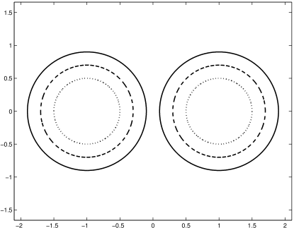
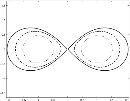
Figure 6: Illustration of Theorem 4.2.

5 Concluding remarks

In this article we investigated properties of lemniscatic maps, i.e., conformal maps from multiply connected domains in the extended complex plane onto lemniscatic domains. We derived a general construction principle of lemniscatic maps in terms of the Riemann map for certain polynomial pre-images of simply connected sets, and we constructed the first (to our knowledge) analytic examples: One for the exterior of $n$ radial slits, and one for the exterior of two disks.

Lemniscatic maps allow the construction of the Faber–Walsh polynomials, which are a direct generalization of the classical Faber polynomials to compact sets consisting of several components. A study of these polynomials is given in our paper [33]. Moreover, we have addressed the numerical computation of lemniscatic maps in [30].

Acknowledgements. We thank Bernd Beckermann for many helpful remarks, and in particular for suggesting to generalize the construction of the conformal map for the radial slit domain in Corollary 3.3 to Theorem 3.1. We also thank the anonymous referees for helpful comments.

References

- [1] V. V. Andreev and T. H. McNicholl, Computing conformal maps of finitely connected domains onto canonical slit domains, Theory Comput. Syst., 50 (2012), pp. 354–369.
- [2] B. Beckermann and L. Reichel, Error estimates and evaluation of matrix functions via the Faber transform, SIAM J. Numer. Anal., 47 (2009), pp. 3849–3883.
- [3] D. Crowdy, The Schwarz-Christoffel mapping to bounded multiply connected polygonal domains, Proc. R. Soc. Lond. Ser. A Math. Phys. Eng. Sci., 461 (2005), pp. 2653–2678.
- [4] , Schwarz-Christoffel mappings to unbounded multiply connected polygonal regions, Math. Proc. Cambridge Philos. Soc., 142 (2007), pp. 319–339.
- [5] D. Crowdy and J. Marshall, Conformal mappings between canonical multiply connected domains, Comput. Methods Funct. Theory, 6 (2006), pp. 59–76.
- [6] J. H. Curtiss, Faber polynomials and the Faber series, Amer. Math. Monthly, 78 (1971), pp. 577–596.
- [7] T. K. DeLillo, Schwarz-Christoffel mapping of bounded, multiply connected domains, Comput. Methods Funct. Theory, 6 (2006), pp. 275–300.
- [8] T. K. DeLillo, T. A. Driscoll, A. R. Elcrat, and J. A. Pfaltzgraff, Computation of multiply connected Schwarz-Christoffel maps for exterior domains, Comput. Methods Funct. Theory, 6 (2006), pp. 301–315.
- [9] , Radial and circular slit maps of unbounded multiply connected circle domains, Proc. R. Soc. Lond. Ser. A Math. Phys. Eng. Sci., 464 (2008), pp. 1719–1737.
- [10] T. K. DeLillo, A. R. Elcrat, and J. A. Pfaltzgraff, Schwarz-Christoffel mapping of multiply connected domains, J. Anal. Math., 94 (2004), pp. 17–47.
- [11] T. K. Delillo and E. H. Kropf, Slit maps and Schwarz-Christoffel maps for multiply connected domains, Electron. Trans. Numer. Anal., 36 (2009/10), pp. 195–223.
- [12] , Numerical computation of the Schwarz-Christoffel transformation for multiply connected domains, SIAM J. Sci. Comput., 33 (2011), pp. 1369–1394.
- [13] S. W. Ellacott, Computation of Faber series with application to numerical polynomial approximation in the complex plane, Math. Comp., 40 (1983), pp. 575–587.
- [14] , A survey of Faber methods in numerical approximation, Comput. Math. Appl. Part B, 12 (1986), pp. 1103–1107.
- [15] H. Grunsky, Über konforme Abbildungen, die gewisse Gebietsfunktionen in elementare Funktionen transformieren. I, Math. Z., 67 (1957), pp. 129–132.
- [16] , Über konforme Abbildungen, die gewisse Gebietsfunktionen in elementare Funktionen transformieren. II, Math. Z., 67 (1957), pp. 223–228.
- [17] , Lectures on theory of functions in multiply connected domains, Vandenhoeck & Ruprecht, Göttingen, 1978.
- [18] M. Hasson, The capacity of some sets in the complex plane, Bull. Belg. Math. Soc. Simon Stevin, 10 (2003), pp. 421–436.
- [19] P. Henrici, Applied and computational complex analysis. Vol. 3, Pure and Applied Mathematics (New York), John Wiley & Sons, Inc., New York, 1986.
- [20] V. Heuveline and M. Sadkane, Arnoldi-Faber method for large non-Hermitian eigenvalue problems, Electron. Trans. Numer. Anal., 5 (1997), pp. 62–76 (electronic).
- [21] J. A. Jenkins, On a canonical conformal mapping of J. L. Walsh, Trans. Amer. Math. Soc., 88 (1958), pp. 207–213.
- [22] T. Koch and J. Liesen, The conformal “bratwurst” maps and associated Faber polynomials, Numer. Math., 86 (2000), pp. 173–191.
- [23] P. Koebe, Abhandlungen zur Theorie der konformen Abbildung, IV. Abbildung mehrfach zusammenhängender schlichter Bereiche auf Schlitzbereiche, Acta Math., 41 (1916), pp. 305–344.
- [24] H. J. Landau, On canonical conformal maps of multiply connected domains, Trans. Amer. Math. Soc., 99 (1961), pp. 1–20.
- [25] W. Magnus, F. Oberhettinger, and R. P. Soni, Formulas and theorems for the special functions of mathematical physics, Third enlarged edition. Die Grundlehren der mathematischen Wissenschaften, Band 52, Springer-Verlag New York, Inc., New York, 1966.
- [26] I. Moret and P. Novati, The computation of functions of matrices by truncated Faber series, Numer. Funct. Anal. Optim., 22 (2001), pp. 697–719.
- [27] , An interpolatory approximation of the matrix exponential based on Faber polynomials, J. Comput. Appl. Math., 131 (2001), pp. 361–380.
- [28] M. M. S. Nasser, Numerical conformal mapping of multiply connected regions onto the second, third and fourth categories of Koebe’s canonical slit domains, J. Math. Anal. Appl., 382 (2011), pp. 47–56.
- [29] , Numerical conformal mapping of multiply connected regions onto the fifth category of Koebe’s canonical slit regions, J. Math. Anal. Appl., 398 (2013), pp. 729–743.
- [30] M. N. S. Nasser, J. Liesen, and O. Sète, Numerical computation of the conformal map onto lemniscatic domains, arXiv:1505.04916, (2015).
- [31] Z. Nehari, Conformal mapping, McGraw-Hill Book Co., Inc., New York, Toronto, London, 1952.
- [32] T. Ransford, Potential theory in the complex plane, vol. 28 of London Mathematical Society Student Texts, Cambridge University Press, Cambridge, 1995.
- [33] O. Sète and J. Liesen, Properties and examples of Faber–Walsh polynomials, arXiv:1502.07633, (2015).
- [34] G. Starke and R. S. Varga, A hybrid Arnoldi-Faber iterative method for nonsymmetric systems of linear equations, Numer. Math., 64 (1993), pp. 213–240.
- [35] P. K. Suetin, Series of Faber polynomials, vol. 1 of Analytical Methods and Special Functions, Gordon and Breach Science Publishers, Amsterdam, 1998.
- [36] F. Tricomi, Elliptische Funktionen, Mathematik und ihre Anwendungen in Physik und Technik, Reihe A, Band 20, Akademische Verlagsgesellschaft Geest & Portig K.-G., Leipzig, 1948.
- [37] J. L. Walsh, On the conformal mapping of multiply connected regions, Trans. Amer. Math. Soc., 82 (1956), pp. 128–146.
- [38] , A generalization of Faber’s polynomials, Math. Ann., 136 (1958), pp. 23–33.
- [39] J. L. Walsh, Selected papers, Springer-Verlag, New York, 2000. Edited by Theodore J. Rivlin and Edward B. Saff.
- [40] E. Wegert, Visual Complex Functions, Birkhäuser/Springer Basel AG, Basel, 2012.
- [41] E. Wegert and G. Semmler, Phase plots of complex functions: a journey in illustration, Notices Am. Math. Soc., 58 (2011), pp. 768–780.
- [42] E. T. Whittaker and G. N. Watson, A course of modern analysis. An introduction to the general theory of infinite processes and of analytic functions: with an account of the principal transcendental functions, Fourth edition. Reprinted, Cambridge University Press, New York, 1962.