Central Trajectories

Abstract

An important task in trajectory analysis is clustering. The results of a clustering are often summarized by a single representative trajectory and an associated size of each cluster. We study the problem of computing a suitable representative of a set of similar trajectories. To this end we define a central trajectory $\mathpzc{C}$, which consists of pieces of the input trajectories, switches from one entity to another only if they are within a small distance of each other, and such that at any time $t$, the point $\mathpzc{C}(t)$ is as central as possible. We measure centrality in terms of the radius of the smallest disk centered at $\mathpzc{C}(t)$ enclosing all entities at time $t$, and discuss how the techniques can be adapted to other measures of centrality. We first study the problem in $\mathbb{R}^{1}$, where we show that an optimal central trajectory $\mathpzc{C}$ representing $n$ trajectories, each consisting of $\tau$ edges, has complexity $\Theta(\tau n^{2})$ and can be computed in $O(\tau n^{2}\log n)$ time. We then consider trajectories in $\mathbb{R}^{d}$ with $d\geq 2$, and show that the complexity of $\mathpzc{C}$ is at most $O(\tau n^{5/2})$ and can be computed in $O(\tau n^{3})$ time.

1 Introduction

A trajectory is a sequence of time-stamped locations in the plane, or more generally in $\mathbb{R}^{d}$. Trajectory data is obtained by tracking the movements of e.g. animals [6, 10, 16], hurricanes [24], traffic [21], or other moving entities [12] over time. Large amounts of such data have recently been collected in a variety of research fields. As a result, there is a great demand for tools and techniques to analyze trajectory data.

One important task in trajectory analysis is clustering: subdividing a large collection of trajectories into groups of “similar” ones. This problem has been studied extensively, and many different techniques are available [7, 14, 15, 20, 25]. Once a suitable clustering has been determined, the result needs to be stored or prepared for further processing. Storing the whole collection of trajectories in each cluster is often not feasible, because follow-up analysis tasks may be computation-intensive. Instead, we wish to represent each cluster by a signature: the number of trajectories in the cluster, together with a representative trajectory which should capture the defining features of all trajectories in the cluster.

Representative trajectories are also useful for visualization purposes. Displaying large amounts of trajectories often leads to visual clutter. Instead, if we show only a number of representative trajectories, this reduces the visual clutter, and allows for more effective data exploration. The original trajectories can still be shown if desired, using the details-on-demand principle in information visualization [23].

Representative trajectories

When choosing a representative trajectory for a group of similar trajectories, the first obvious choice would be to pick one of the trajectories in the group. However, one can argue that no single element in a group may be a good representative, e.g. because each individual trajectory has some prominent feature that is not shared by the rest (see Fig. 1), or no trajectory is sufficiently in the middle all the time. On the other hand, it is desirable to output a trajectory that does consist of pieces of input trajectories, because otherwise the representative trajectory may display behaviour that is not present in the input, e.g. because of contextual information that is not available to the algorithm (see Fig. 1).

Figure 1: (a) Every trajectory has a peculiarity that is not representative for the set. (b) Taking, for example, the pointwise average of a set of trajectories may result in one that ignores context.

To determine what a good representative trajectory of a group of similar trajectories is, we identify two main categories: time-dependent and time-independent representatives. Trajectories are typically collected as a discrete sequence of time-stamped locations. By linearly interpolating the locations we obtain a continuous piecewise-linear curve as the image of the function. Depending on the application, we may be interested in the curve with attached time stamps (say, when studying a flock of animals that moved together) or in just the curve (say, when considering hikers that took the same route, but possibly at different times and speeds).

When time is not important, one can select a representative based directly on the geometry or topology of the set of curves [8, 18]. When time is important, we would like to have the property that at each time $t$ our representative point $c(t)$ is a good representative of the set of points $P(t)$. To this end, we may choose any static representative point of a point set, for which many examples are available: the Fermat-Weber point (which minimizes the sum of distances to the points in $P$), the center of mass (which minimizes the sum of squared distances), or the center of the smallest enclosing circle (which minimizes the distance to the farthest point in $P$).

Central trajectories

In this work, we focus on time-dependent measures based on static concepts of centrality. We choose the distance to the farthest point, but discuss in Section 4 how our results can be adapted to other measures.

Ideally, we would output a trajectory $\mathpzc{C}$ such that at any time $t$, $\mathpzc{C}(t)$ is the point (entity) that is closest to its farthest entity. Unfortunately, when the entities move in $\mathbb{R}^{d}$ for $d>1$, this may cause discontinuities. Such discontinuities are unavoidable: if we insist that the output trajectory consists of pieces of input trajectories and is continuous, then in general, there will be no opportunities to switch from one trajectory to another, and we are effectively choosing one of the input trajectories again. At the same time, we do not want to output a trajectory with arbitrarily large discontinuities. An acceptable compromise is to allow discontinuities, or jumps, but only over small distances, controlled by a parameter $\varepsilon$. We note that this problem of discontinuities shows up for time-independent representatives for entities moving in $\mathbb{R}^{d}$, with $d\geq 3$, as well, because the traversed curves generally do not intersect.

Related work

Buchin et al. [8] consider the problem of computing a median trajectory for a set of trajectories without time information. Their method produces a trajectory that consists of pieces of the input. Agarwal et al. [1] consider trajectories with time information and compute a representative trajectory that follows the median (in $\mathbb{R}^{1}$) or a point of high depth (in $\mathbb{R}^{2}$) of the input entities. The resulting trajectory does not necessarily stay close to the input trajectories. They give exact and approximate algorithms. Durocher and Kirkpatrick [13] observe that a trajectory minimizing the sum of distances to the other entities is unstable, in the sense that arbitrarily small movement of the entities may cause an arbitrarily large movement in the location of the representative entity. They proceed to consider alternative measures of centrality, and define the projection median, which they prove is more stable. Basu et al. [4] extend this concept to higher dimensions.

Problem description

We are given a set $\mathcal{X}$ of $n$ entities, each moving along a piecewise linear trajectory in $\mathbb{R}^{d}$ consisting of $\tau$ edges. We assume that all trajectories have their vertices at the same times, i.e. times $t_{0},..,t_{\tau}$. Fig. 2 shows an example.

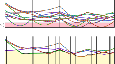
Figure 2: (a) Two views of five moving entities and their trajectories. (b) On the top the pairwise distances between the entities as a function over time. On the bottom the functions $D_{\sigma}$, and in yellow the area representing $\mathcal{D}(\mathpzc{C})$.

For an entity $\sigma$, let $\sigma(t)$ denote the position of $\sigma$ at time $t$. With slight abuse of notation we will write $\sigma$ for both entity $\sigma$ and its trajectory. At a given time $t$, we denote the distance from $\sigma$ to the entity farthest away from $\sigma$ by $D_{\sigma}(t)=D(\sigma,t)=\max_{\psi\in\mathcal{X}}\|\sigma(t)\psi(t)\|$, where $\|pq\|$ denotes the Euclidean distance between points $p$ and $q$ in $\mathbb{R}^{d}$. Fig. 2 illustrates the pairwise distances and resulting $D$ functions for five example trajectories. For ease of exposition, we assume that the trajectories are in general position: that is, no three trajectories intersect in the same point, and no two pairs of entities are at distance $\varepsilon$ from each other at the same time.

A trajectoid is a function that maps time to the set of entities $\mathcal{X}$, with the restriction that at discontinuities the distance between the entities involved is at most $\varepsilon$. Intuitively, a trajectoid corresponds to a concatenation of pieces of the input trajectories in such a way that two consecutive pieces match up in time, and the end point of the former piece is within distance $\varepsilon$ from the start point of the latter piece. In Fig. 2, a trajectoid may switch between a pair of entities when their pairwise distance function lies in the bottom strip of height $\varepsilon$. More formally, for a trajectoid $\mathpzc{T}$ we have that

• at any time $t$, $\mathpzc{T}(t)=\sigma$ for some $\sigma\in\mathcal{X}$, and

• at every time $t$ where $\mathpzc{T}$ has a discontinuity, that is, $\mathpzc{T}$ jumps from entity $\sigma$ to entity $\psi$, we have that $\|\sigma(t)\psi(t)\|\leq\varepsilon$.

Note that this definition still allows for a series of jumps within an arbitrarily short time interval $[t,t+\delta]$, essentially simulating a jump over distances larger than $\varepsilon$. To make the formulation cleaner, we slightly weaken the second condition, and allow a trajectoid to have discontinuities with a distance larger than $\varepsilon$, provided that such a large jump can be realized by a sequence of small jumps, each of distance at most $\varepsilon$. When it is clear from the context, we will write $\mathpzc{T}(t)$ instead of $\mathpzc{T}(t)(t)$ to mean the location of entity $\mathpzc{T}(t)$ at time $t$. We now wish to compute a trajectoid $\mathpzc{C}$ that minimizes the function

$$\mathcal{D}(\mathpzc{T})=\int_{t_{0}}^{t_{\tau}}D(\mathpzc{T},t)\,\mathrm{d}t.$$

So, at any time $t$, all entities lie in a disk of radius $D(\mathpzc{C},t)$ centered at $\mathpzc{C}(t)$.

Outline and results

We first study the situation where entities move in $\mathbb{R}^{1}$. In Section 2 we show that the worst case complexity of a central trajectory in $\mathbb{R}^{1}$ is $\Theta(\tau n^{2})$, and that we can compute one in $O(\tau n^{2}\log n)$ time. We then extend our approach to entities moving in $\mathbb{R}^{d}$, for any constant $d$, in Section 3. For this case, we prove that the maximal complexity of a central trajectory $\mathpzc{C}$ is $O(\tau n^{5/2})$. Computing $\mathpzc{C}$ takes $O(\tau n^{3})$ time and requires $O(\tau n^{2}\log n)$ working space. We briefly discuss various extensions to our approach in Section 4. Omitted proofs can be found in Appendix LABEL:app:Omitted_Proofs.

Even though we do not expect this to happen in practice, the worst case complexity of our central trajectories can be significantly higher than the input size. If this occurs, we can use traditional line simplification algorithms like Imai and Iri [19] to simplify the resulting central trajectory. This gives us a representative that still is always close —for instance within distance $2\varepsilon$— to one of the input trajectories. Alternatively, we can use dynamic-programming combined with our methods to enforce the output trajectory to have at most $k$ vertices, for any $k$, and always be on the input trajectories. Computing such a central trajectory is more expensive than our current algorithms, however. Furthermore, enforcing a low output complexity may not be necessary. For example, in applications like visualization, the number of trajectories shown often has a larger impact visual clutter than the length or complexity of the individual trajectories. It may be easier to follow a single trajectory that has many vertices than to follow many trajectories that have fewer vertices each.

2 Entities moving in $\mathbb{R}^{1}$

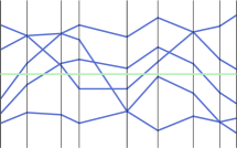
Figure 3: (a) A set of trajectories and the ideal trajectory $\mathpzc{I}$. The breakpoints in the ideal trajectory partition time into $O(n\tau)$ intervals. (b) The trajectories after transforming $\mathpzc{I}$ to a horizontal line.

Let $\mathcal{X}$ be the set of entities moving in $\mathbb{R}^{1}$. The trajectories of these entities can be seen as polylines in $\mathbb{R}^{2}$: we associate time with the horizontal axis, and $\mathbb{R}^{1}$ with the vertical axis (see Fig. 3). We observe that the distance between two points $p$ and $q$ in $\mathbb{R}^{1}$ is simply their absolute difference, that is, $\|pq\|=|p-q|$.

Let $\mathpzc{I}$ be the ideal trajectory, that is, the trajectory that minimizes $\mathcal{D}$ but is not restricted to lie on the input trajectories. It follows that at any time $t$, $\mathpzc{I}(t)$ is simply the average of the highest entity $\mathpzc{U}(t)$ and the lowest entity $\mathpzc{L}(t)$. We further subdivide each time interval $J_{i}=[t_{i},t_{i+1}]$ into elementary intervals, such that $\mathpzc{I}$ is a single line segment inside each elementary interval.

Lemma 1.

The total number of elementary intervals is $\tau(n+2)$.

Proof. The ideal trajectory $\mathpzc{I}$ changes direction when $\mathpzc{U}(t)$ or $\mathpzc{L}(t)$ changes. During a single interval $[t_{i},t_{i+1}]$ all entities move along lines, so $\mathpzc{U}$ and $\mathpzc{L}$ are the upper and lower envelope of a set of $n$ lines. So by standard point-line duality, $\mathpzc{U}$ and $\mathpzc{L}$ correspond to the upper and lower hull of $n$ points. The summed complexity of the upper and lower hull is at most $n+2$. ∎

We assume without loss of generality that within each elementary interval $\mathpzc{I}$ coincides with the $x$-axis. To simplify the description of the proofs and algorithms, we also assume that the entities never move parallel to the ideal trajectory, that is, there are no horizontal edges.

Lemma 2.

$\mathpzc{C}$ is a central trajectory in $\mathbb{R}^{1}$ if and only if it minimizes the function

$$\mathcal{D}^{\prime}(\mathpzc{T})=\int_{t_{0}}^{t_{\tau}}|\mathpzc{T}(t)|\,\mathrm{d}t.$$

Proof. A central trajectory $\mathpzc{C}$ is a trajectoid that minimizes the function

$$\mathcal{D}(\mathpzc{T}) =\int_{t_{0}}^{t_{\tau}}D(\mathpzc{T},t)\,\mathrm{d}t=\int_{t_{0}}^{t_{\tau}}\max_{\psi\in\mathcal{X}}\|\mathpzc{T}(t)\psi(t)\|\,\mathrm{d}t=\int_{t_{0}}^{t_{\tau}}\max_{\psi\in\mathcal{X}}|\mathpzc{T}(t)-\psi(t)|\,\mathrm{d}t$$

$$=\int_{t_{0}}^{t_{\tau}}\max\{|\mathpzc{T}(t)-\mathpzc{U}(t)|,|\mathpzc{T}(t)-\mathpzc{L}(t)|\}\,\mathrm{d}t.$$

Since $(\mathpzc{U}(t)+\mathpzc{L}(t))/2=0$, we have that $|\mathpzc{T}(t)-\mathpzc{U}(t)|>|\mathpzc{T}(t)-\mathpzc{L}(t)|$ if and only if $\mathpzc{T}(t)<0$. So, we split the integral, depending on $\mathpzc{T}(t)$, giving us

$$\mathcal{D}(\mathpzc{T}) =\int_{t_{0}\leq t\leq t_{\tau}\land\mathpzc{T}(t)\geq 0}\mathpzc{T}(t)-\mathpzc{L}(t)\,\mathrm{d}t+\int_{t_{0}\leq t\leq t_{\tau}\land\mathpzc{T}(t)<0}\mathpzc{U}(t)-\mathpzc{T}(t)\,\mathrm{d}t$$

$$=\int_{t_{0}\leq t\leq t_{\tau}\land\mathpzc{T}(t)\geq 0}\mathpzc{T}(t)\,\mathrm{d}t-\int_{t_{0}\leq t\leq t_{\tau}\land\mathpzc{T}(t)\geq 0}\mathpzc{L}(t)\,\mathrm{d}t\leavevmode\nobreak\ +$$

$$\quad\int_{t_{0}\leq t\leq t_{\tau}\land\mathpzc{T}(t)<0}\mathpzc{U}(t)\,\mathrm{d}t-\int_{t_{0}\leq t\leq t_{\tau}\land\mathpzc{T}(t)<0}\mathpzc{T}(t)\,\mathrm{d}t.$$

We now use that $-\int_{\mathpzc{T}(t)<0}\mathpzc{T}(t)=\int_{\mathpzc{T}(t)<0}|\mathpzc{T}(t)|$, and that $-\int\mathpzc{L}(t)=\int\mathpzc{U}(t)$ (since $(\mathpzc{U}(t)+\mathpzc{L}(t))/2=0$). After rearranging the terms we then obtain

$$\mathcal{D}(\mathpzc{T}) =\int_{t_{0}\leq t\leq t_{\tau}\land\mathpzc{T}(t)\geq 0}\mathpzc{T}(t)\,\mathrm{d}t+\int_{t_{0}\leq t\leq t_{\tau}\land\mathpzc{T}(t)<0}|\mathpzc{T}(t)|\,\mathrm{d}t\leavevmode\nobreak\ +$$

$$\quad\int_{t_{0}\leq t\leq t_{\tau}\land\mathpzc{T}(t)\geq 0}\mathpzc{U}(t)\,\mathrm{d}t+\int_{t_{0}\leq t\leq t_{\tau}\land\mathpzc{T}(t)<0}\mathpzc{U}(t)\,\mathrm{d}t$$

$$=\int_{t_{0}\leq t\leq t_{\tau}}|\mathpzc{T}(t)|\,\mathrm{d}t\leavevmode\nobreak\ +\int_{t_{0}\leq t\leq t_{\tau}}\mathpzc{U}(t)\,\mathrm{d}t.$$

The last term is independent of $\mathpzc{T}$, so we have $\mathcal{D}(\mathpzc{T})=\mathcal{D}^{\prime}(\mathpzc{T})+c$, for some $c\in\mathbb{R}$. The lemma follows. ∎

By Lemma 2 a central trajectory $\mathpzc{C}$ is a trajectoid that minimizes the area $\mathcal{D}^{\prime}(\mathpzc{T})$ between $\mathpzc{T}$ and the ideal trajectory $\mathpzc{I}$. Hence, we can focus on finding a trajectoid that minimizes $\mathcal{D}^{\prime}$.

2.1 Complexity

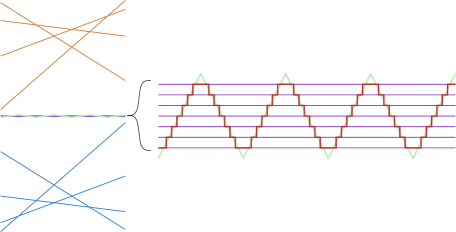
Figure 4: Lower bound construction that shows that $\mathcal{C}$ (red) may have quadratic complexity. The ideal trajectory $\mathpzc{I}$ is shown in green.

Lemma 3.

For a set of $n$ trajectories in $\mathbb{R}^{1}$, each with vertices at times $t_{0},..,t_{\tau}$, a central trajectory $\mathpzc{C}$ may have worst case complexity $\Omega(\tau n^{2})$.

Proof. We describe a construction for the entities that shows that within a single time interval $J=[t_{i},t_{i+1}]$ the complexity of $\mathpzc{C}$ may be $\Omega(n^{2})$. Repeating this construction $\tau$ times gives us $\Omega(\tau n^{2})$ as desired.

Within $J$ the entities move linearly. So we construct an arrangement $\mathcal{A}$ of lines that describes the motion of all entities. We place $m=n/3$ lines such that the upper envelope of $\mathcal{A}$ has linear complexity. We do the same for the lower envelope. We position these lines such that the ideal trajectory $\mathpzc{I}$—which is the average of the upper and lower envelope— makes a vertical “zigzagging” pattern (see Fig. 4). The remaining set $H$ of $m$ lines are horizontal. Two consecutive lines are placed at (vertical) distance at most $\varepsilon$. We place all lines such that they all intersect $\mathpzc{I}$. It follows that $\mathpzc{C}$ jumps $O(n^{2})$ times between the lines in $H$. The lemma follows. ∎

Two entities $\sigma$ and $\psi$ are $\varepsilon$-connected at time $t$ if there is a sequence $\sigma=\sigma_{0},..,\sigma_{k}=\psi$ of entities such that for all $i$, $\sigma_{i}$ and $\sigma_{i+1}$ are within distance $\varepsilon$ of each other at time $t$. A subset $\mathcal{X}^{\prime}\subseteq\mathcal{X}$ of entities is $\varepsilon$-connected at time $t$ if all entities in $\mathcal{X}^{\prime}$ are pairwise $\varepsilon$-connected at time $t$. The set $\mathcal{X}^{\prime}$ is $\varepsilon$-connected during an interval $I$, if they are $\varepsilon$-connected at any time $t\in I$. We now observe:

Observation 4.

$\mathpzc{C}$ can jump from entity $\sigma$ to $\psi$ at time $t$ if and only if $\sigma$ and $\psi$ are $\varepsilon$-connected at time $t$.

At any time $t$, we can partition $\mathcal{X}$ into maximal sets of $\varepsilon$-connected entities. The central trajectory $\mathpzc{C}$ must be in one of such maximal sets $\mathcal{X}^{\prime}$: it uses the trajectory of an entity $\sigma\in\mathcal{X}^{\prime}$ (at time $t$), if and only if $\sigma$ is the entity from $\mathcal{X}^{\prime}$ closest to $\mathpzc{I}$. More formally, let $f_{\sigma}(t)=|\sigma(t)|$, and let $\mathpzc{L}(\mathcal{F})=\min_{f\in\mathcal{F}}f$ denote the lower envelope of a set of functions $\mathcal{F}$.

Observation 5.

Let $\mathcal{X}^{\prime}\ni\sigma$ be a set of entities that is $\varepsilon$-connected during interval $J$, and assume that $\mathpzc{C}\in\mathcal{X}^{\prime}$ during $J$. For any time $t\in J$, we have that $\mathpzc{C}(t)=\sigma(t)$ if and only if $f_{\sigma}$ is on the lower envelope of the set $\mathcal{F}^{\prime}=\{f_{\psi}\mid\psi\in\mathcal{X}^{\prime}\}$ at time $t$, that is, $f_{\sigma}(t)=\mathpzc{L}(\mathcal{F})(t)$.

Let $\mathcal{X}_{1},..,\mathcal{X}_{m}$, denote a collection of maximal sets of entities that are $\varepsilon$-connected during time intervals $J_{1},..,J_{m}$, respectively. Let $\mathcal{F}_{i}=\{f_{\sigma}\mid\sigma\in\mathcal{X}_{i}\}$, and let $\mathpzc{L}_{i}$ be the lower envelope $\mathpzc{L}(\mathcal{F}_{i})$ of $\mathcal{F}_{i}$ restricted to interval $J_{i}$. A lower envelope $\mathpzc{L}_{i}$ has a break point at time $t$ if $f_{\sigma}(t)=f_{\psi}(t)$, for $\sigma,\psi\in\mathcal{X}_{i}$. There are two types of break points: (i) $\sigma(t)=\psi(t)$, or (ii) $\sigma(t)=-\psi(t)$. At events of type (i) the modified trajectories of $\sigma$ and $\psi$ intersect. At events of the type (ii), $\sigma$ and $\psi$ are equally far from $\mathpzc{I}$, but on different sides of $\mathpzc{I}$. Let $B=\{(t,\sigma,\psi)\mid\mathpzc{L}_{i}(t)=f_{\sigma}(t)=f_{\psi}(t)\land i\in\{1,..,m\}\}$ denote the collection of break points from all lower envelopes $\mathpzc{L}_{1},..,\mathpzc{L}_{m}$.

Lemma 6.

Consider a triplet $(t,\sigma,\psi)\in B$. There is at most one lower envelope $\mathpzc{L}_{i}$ such that $t$ is a break point in $\mathpzc{L}_{i}$.

Proof. Assume by contradiction that $t$ is a break point in both $\mathpzc{L}_{i}$ and $\mathpzc{L}_{j}$. At any time $t$, an entity can be in at most one maximal set $\mathcal{X}_{\ell}$. So if $\mathcal{X}_{i}$ and $\mathcal{X}_{j}$ share either entity $\sigma$ or $\psi$, then the intervals $J_{i}$ and $J_{j}$ are disjoint. It follows $t$ cannot lie in both intervals, and thus cannot be a break point in both $\mathpzc{L}_{i}$ and $\mathpzc{L}_{j}$. Contradiction. ∎

Lemma 7.

Let $\mathcal{A}$ be an arrangement of $n$ lines, describing the movement of $n$ entities during an elementary interval $J$. If there is a break point $(t,\sigma,\psi)\in B$, with $t\in J$, of type (ii), then $\sigma(t)$ and $\psi(t)$ lie on the boundary $\partial\mathcal{Z}$ of the zone $\mathcal{Z}$ of $\mathpzc{I}$ in $\mathcal{A}$.

Proof. Let $\mathcal{X}_{j}$ be the maximal $\varepsilon$-connected set containing $\sigma$ and $\psi$, and assume without loss of generality that $f_{\sigma}(t)=\sigma(t)=-\psi(t)=f_{\psi}(t)$. Now, assume by contradiction that $\sigma$ is not on $\partial\mathcal{Z}$ at time $t$ (the case that $\psi(t)$ is not on $\partial\mathcal{Z}$ is symmetric). This means that there is an entity $\rho$ with $0\leq\rho(t)<\sigma(t)$. If $\rho\in\mathcal{X}_{j}$, this contradicts that $f_{\sigma}(t)$ was on the lower envelope of $\mathcal{X}_{j}$ at time $t$. So $\rho$ is not $\varepsilon$-connected to $\sigma$ at time $t$. Hence, their distance is at least $\varepsilon$. We then have $\sigma(t)>\rho(t)+\varepsilon>\varepsilon$. It now follows that $\sigma$ and $\psi$ cannot be $\varepsilon$-connected at time $t$: the distance between $\sigma$ and $\psi$ is bigger than $\varepsilon$ so they are not directly connected, and $f_{\sigma}$ and $f_{\psi}$ are on $\mathpzc{L}_{j}$, so there are also no other entities in $\mathcal{X}_{j}$ through which they can be $\varepsilon$-connected. Contradiction. ∎

Lemma 8.

Let $\mathcal{A}$ be an arrangement of $n$ lines, describing the movement of $n$ entities during an elementary interval $J$. The total number of break points $(t,\sigma,\phi)\in B$, with $t\in J$, of type (ii) is at most $6.5n$.

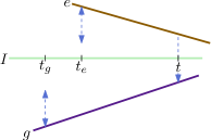
Figure 5: The jumps of $\mathpzc{L}$ (dashed arrows) involving edges $e$ and $g$.

Proof. By Lemma 6 all break points can be charged to exactly one set $\mathcal{X}_{j}$. From Lemma 7 it follows that break points of type (ii) involve only entities whose lines in $\mathcal{A}$ participate in the zone of $\mathpzc{I}$.

Let $E$ be the set of edges of $\partial\mathcal{Z}$. We have that $|E|\leq 5.5n$ [5, 22]. We now split every edge that intersects $\mathpzc{I}$, at the intersection point. Since every line intersects $\mathpzc{I}$ at most once, this means the number of edges in $E$ increases to $6.5n$. For every pair of edges $(e,g)$, that lie on opposite sides of $\mathpzc{I}$, there is at most one time $t$ where a lower envelope $\mathpzc{L}=\mathpzc{L}_{j}$, for some $j$, has a break point of type (ii).

Consider a break point of type (ii), that is, a time $t$ such that $\mathpzc{L}$ switches (jumps) from an entity $\sigma$ to an entity $\psi$, with $\sigma$ and $\psi$ on opposite sides of $\mathpzc{I}$. Let $e\in E$ and $g\in E$ be the edges containing $\sigma(t)$ and $\psi(t)$, respectively. If the arriving edge $g$ has not been charged before, we charge the jump to $g$. Otherwise, we charge it to $e$. We continue to show that every edge in $E$ is charged at most once. Since $E$ has at most $6.5n$ edges, the number of break points of type (ii) is also at most $6.5n$.

We now show that either $e$ or $g$ has not been charged before. Assume, by contradiction, that both $e$ and $g$ have been charged before time $t$, at times $t_{e}$ and $t_{g}$, respectively. Consider the case that $t_{g}<t_{e}$ (see Fig. 5). At time $t_{e}$, the lower envelope $\mathpzc{L}$ jumps from an edge $h$ onto $e$ or vice versa. Since there is a jump involving edge $g$ at time $t_{g}$ and one at time $t$ it follows that at time $t_{e}$, $g$ is the closest edge in $E$ opposite to $e$. Hence, $h=g$. This means we jump twice between $e$ and $g$. Contradiction. The case $t_{e}<t_{g}$ is symmetrical and the case $t_{e}=t_{g}$ cannot occur. It follows that $e$ or $g$ was not charged before time $t$, and thus all edges in $E$ are charged at most once. ∎

Lemma 9.

The total complexity of all lower envelopes $\mathpzc{L}_{1},..,\mathpzc{L}_{m}$ on $[t_{i},t_{i+1}]$ is $O(n^{2})$.

Proof. The break points in the lower envelopes are either of type (i) or of type (ii). We now show that there are at most $O(n^{2})$ break points of either type.

The break points of type (i) correspond to intersections between the trajectories of two entities. Within interval $[t_{i},t_{i+1}]$ the entities move along lines, hence there are at most $O(n^{2})$ such intersections. By Lemma 6 all break points can be charged to exactly one set $\mathcal{X}_{i}$. It follows that the total number of break points of type (i) is $O(n^{2})$.

To show that the number of events of the second type is at most $O(n^{2})$ as well we divide $[t_{i},t_{i+1}]$ in $O(n)$ elementary intervals such that $\mathpzc{I}$ coincides with the $x$-axis. By Lemma 8 each such elementary interval contains at most $O(n)$ break points of type (ii). ∎

Theorem 10.

Given a set of $n$ trajectories in $\mathbb{R}^{1}$, each with vertices at times $t_{0},..,t_{\tau}$, a central trajectory $\mathpzc{C}$ has worst case complexity $O(\tau n^{2})$.

Proof. A central trajectory $\mathpzc{C}$ is a piecewise function. From Observations 4 and 5 it now follows that $\mathpzc{C}$ has a break point at time $t$ only if (a) two subsets of entities become $\varepsilon$-connected or $\varepsilon$-disconnected, or (b) the lower envelope of a set of $\varepsilon$-connected entities has a break point at time $t$. Within a single time interval $J_{i}=[t_{i},t_{i+1}]$ there are at most $O(n^{2})$ times when two entities are at distance exactly $\varepsilon$. Hence, the number of events of type (a) during interval $J_{i}$ is also $O(n^{2})$. By Lemma 9 the total complexity of all lower envelopes of $\varepsilon$-connected sets during $J_{i}$ is also $O(n^{2})$. Hence, the number of break points of type (b) within interval $J_{i}$ is also $O(n^{2})$. The theorem follows. ∎

2.2 Algorithm

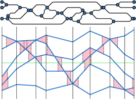
Figure 6: The Reeb graph for the moving entities from Fig. 3. The dashed lines indicate that two entities are at distance $\varepsilon$.

We now present an algorithm to compute a trajectoid $\mathpzc{C}$ minimizing $\mathcal{D}^{\prime}$. By Lemma 2 such a trajectoid is a central trajectory. The basic idea is to construct a weighted (directed acyclic) graph that represents a set of trajectoids containing an optimal trajectoid. We can then find $\mathpzc{C}$ by computing a minimum weight path in this graph.

The graph that we use is a weighted version of the Reeb graph that Buchin et al. [9] use to model the trajectory grouping structure. We review their definition here. The Reeb graph $\mathcal{R}$ is a directed acyclic graph. Each edge $e=(u,v)$ of $\mathcal{R}$ corresponds to a maximal subset of entities $C_{e}\subseteq\mathcal{X}$ that is $\varepsilon$-connected during the time interval $[t_{u},t_{v}]$. The vertices represent times at which the sets of $\varepsilon$-connected entities change, that is, the times at which two entities $\sigma$ and $\psi$ are at distance $\varepsilon$ from each other and the set containing $\sigma$ merges with or splits from the set containing $\psi$. See Fig. 6 for an illustration.

By Observation 4 a central trajectory $\mathpzc{C}$ can jump from $\sigma$ to $\psi$ if and only if $\sigma$ and $\psi$ are $\varepsilon$-connected, that is, if $\sigma$ and $\psi$ are in the same component $C_{e}$ of edge $e$. From Observation 5 it follows that on each edge $e$, $\mathpzc{C}$ uses only the trajectories of entities $\sigma$ for which $f_{\sigma}$ occurs on the lower envelope of the functions $\mathcal{F}_{e}=\{f_{\sigma}\mid\sigma\in C_{e}\}$. Hence, we can then express the cost for $\mathpzc{C}$ using edge $e$ by

$$\omega_{e}=\int_{t_{u}}^{t_{v}}\mathpzc{L}(\mathcal{F}_{e})(t)\,\mathrm{d}t.$$

It now follows that $\mathpzc{C}$ follows a path in the Reeb graph $\mathcal{R}$, that is, the set of trajectoids represented by $\mathcal{R}$ contains a trajectoid minimizing $\mathcal{D}^{\prime}$. So we can compute a central trajectory by finding a minimum weight path in $\mathcal{R}$ from a source to a sink.

Analysis

First we compute the Reeb graph as defined by Buchin et al. [9]. This takes $O(\tau n^{2}\log n)$ time. Second we compute the weight $\omega_{e}$ for each edge $e$. The Reeb graph $\mathcal{R}$ is a DAG, so once we have the edge weights, we can use dynamic programming to compute a minimum weight path in $O(|\mathcal{R}|)=O(\tau n^{2})$ time. So all that remains is to compute the edge weights $\omega_{e}$. For this, we need the lower envelope $\mathpzc{L}_{e}$ of each set $\mathcal{F}_{e}$ on the interval $J_{e}$. To compute the lower envelopes, we need the ideal trajectory $\mathpzc{I}$, which we can compute $\mathpzc{I}$ in $O(\tau n\log n)$ time by computing the lower and upper envelope of the trajectories in each time interval $[t_{i},t_{i+1}]$.

Lemma 9 implies that the total complexity of all lower envelopes is $O(\tau n^{2})$. To compute them we have two options. We can simply compute the lower envelope from scratch for every edge of $\mathcal{R}$. This takes $O(\tau n^{2}\cdot n\log n)=O(\tau n^{3}\log n)$ time. Instead, for each time interval $J_{i}=[t_{i},t_{i+1}]$, we compute the arrangement $\mathcal{A}$ representing the modified trajectories on the interval $J_{i}$, and use it to trace $\mathpzc{L}_{e}$ in $\mathcal{A}$ for every edge $e$ of $\mathcal{R}$.

An arrangement of $m$ line segments can be built in $O(m\log m+A)$ time, where $A$ is the output complexity [2]. In total $\mathcal{A}$ consists of $O(n^{2})$ line segments: $n+2$ per entity. Since each pair of trajectories intersects at most once during $J_{i}$, we have that $A=O(n^{2})$. Thus, we can build $\mathcal{A}$ in $O(n^{2}\log n)$ time. The arrangement $\mathcal{A}$ represents all break points of type (i), of all functions $f_{\sigma}$. We now compute all pairs of points in $\mathcal{A}$ corresponding to break points of type (ii). We do this in $O(n^{2})$ time by traversing the zone of $\mathpzc{I}$ in $\mathcal{A}$.

We now trace the lower envelopes through $\mathcal{A}$: for each edge $e=(u,v)$ in the Reeb graph with $J_{e}\subseteq J_{i}$, we start at the point $\sigma(t_{u})$, $\sigma\in C_{e}$, that is closest to $\mathpzc{I}$, and then follow the edges in $\mathcal{A}$ corresponding to $\mathpzc{L}_{e}$, taking care to jump when we encounter break points of type (ii). Our lower envelopes are all disjoint (except at endpoints), so we traverse each edge in $\mathcal{A}$ at most once. The same holds for the jumps. We can avoid costs for searching for the starting point of each lower envelope by tracing the lower envelopes in the right order: when we are done tracing $\mathpzc{L}_{e}$, with $e=(u,v)$, we continue with the lower envelope of an outgoing edge of vertex $v$. If $v$ is a split vertex where $\sigma$ and $\psi$ are at distance $\varepsilon$, then the starting point of the lower envelope of the other edge is either $\sigma(t_{v})$ or $\psi(t_{v})$, depending on which of the two is farthest from $\mathpzc{I}$. It follows that when we have $\mathcal{A}$ and the list of break points of type (ii), we can compute all lower envelopes in $O(n^{2})$ time. We conclude:

Theorem 11.

Given a set of $n$ trajectories in $\mathbb{R}^{1}$, each with vertices at times $t_{0},..,t_{\tau}$, we can compute a central trajectory $\mathpzc{C}$ in $O(\tau n^{2}\log n)$ time using $O(\tau n^{2})$ space.

A central trajectory without jumps

When our entities move in $\mathbb{R}^{1}$, it is not yet necessary to have discontinuities in $\mathpzc{C}$, i.e. we can set $\varepsilon=0$. In this case we can give a more precise bound on the complexity of $\mathpzc{C}$, and we can use a slightly easier algorithm. The details can be found in Appendix A.

3 Entities moving in $\mathbb{R}^{d}$

In the previous section, we used the ideal trajectory $\mathpzc{I}$, which minimizes the distance to the farthest entity, ignoring the requirement to stay on an input trajectory. The problem was then equivalent to finding a trajectoid that minimizes the distance to the ideal trajectory. In $\mathbb{R}^{d}$, with $d>1$, however, this approach fails, as the following example shows.

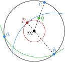
Figure 7: Point $p$ is closest to the ideal point $m$, however the smallest enclosing disk centered at $q$ is smaller than that of $p$.

Observation 12.

Let $P$ be a set of points in $\mathbb{R}^{2}$. The point in $P$ that minimizes the distance to the ideal point (i.e., the center of the smallest enclosing disk of $P$) is not necessarily the same as the point in $P$ that minimizes the distance to the farthest point in $P$.

Proof. See Fig. 7. Consider three points $a$, $b$ and $c$ at the corners of an equilateral triangle, and two points $p$ and $q$ close to the center $m$ of the circle through $a$, $b$ and $c$. Now $p$ is closer to $m$ than $q$, yet $q$ is closer to $b$ than $p$ (and $q$ is as far from $a$ as from $b$). ∎

3.1 Complexity

It follows from Lemma 3 that the complexity of a central trajectory for entities moving in $\mathbb{R}^{d}$ is at least $\Omega(\tau n^{2})$. In this section, we prove that the complexity of $\mathpzc{C}$ within a single time interval $[t_{i},t_{i+1}]$ is at most $O(n^{5/2})$. Thus, the complexity over all $\tau$ time intervals is $O(\tau n^{5/2})$.

Let $\mathcal{F}$ denote the collection of functions $D_{\sigma}$, for $\sigma\in\mathcal{X}$. We partition time into intervals $J^{\prime}_{1},..,J^{\prime}_{k^{\prime}}$ such that in each interval $J^{\prime}_{i}$ all functions $D_{\sigma}$ restricted to $J^{\prime}_{i}$ are simple, that is, they consist of just one piece. We now show that each function $D_{\sigma}$ consists of at most $\tau(2n-1)$ pieces, and thus the total number of intervals is at most $O(\tau n^{2})$. See Fig. 2 for an illustration.

Lemma 13.

Each function $D_{\sigma}$ is piecewise hyperbolic and consists of at most $\tau(2n-1)$ pieces.

Proof. Consider a time interval $J_{i}=[t_{i},t_{i+1}]$. For any entity $\psi$ and any time $t\in J_{i}$, the function $\|\sigma(t)\psi(t)\|=\sqrt{at^{2}+bt+c}$, with $a,b,c\in\mathbb{R}$, is hyperbolic in $t$. Each pair of such functions can intersect at most twice. During $J_{i}$, $D_{\sigma}$ is the upper envelope of these functions, so it consists of $\lambda_{2}(n)$ pieces, where $\lambda_{s}$ denotes the maximum complexity of a Davenport-Schinzel sequence of order $s$ [3]. We have $\lambda_{2}(n)=2n-1$, so the lemma follows. ∎

Lemma 14.

The total number of intersections of all functions in $\mathcal{F}$ is at most $O(\tau n^{3})$.

Proof. Fix a pair of entities $\sigma,\psi$. By Lemma 13 there are at most $\tau(2n-1)$ time intervals $J$, such that $D_{\sigma}$ restricted to $J$ is simple. The same holds for $D_{\psi}$. So, there are at most $\tau(4n-2)$ intervals in which both $D_{\sigma}$ and $D_{\psi}$ are simple (and hyperbolic). In each interval $D_{\sigma}$ and $D_{\psi}$ intersect at most twice. ∎

We again observe that $\mathpzc{C}$ can only jump from one entity to another if they are $\varepsilon$-connected. Hence, Observation 4 holds entities moving in $\mathbb{R}^{d}$ as well. As before, this means that at any time $t$, we can partition $\mathcal{X}$ into maximal sets of $\varepsilon$-connected entities. Let $\mathcal{X}^{\prime}\ni\sigma$ be a maximal subset of $\varepsilon$-connected entities at time $t$. This time, a central trajectory $\mathpzc{C}$ uses the trajectory of entity $\sigma$ at time $t$, if and only if $\sigma$ is the entity from $\mathcal{X}^{\prime}$ whose function $\mathcal{D}_{\sigma}$ is minimal. Hence, if we define $f_{\sigma}=D_{\sigma}$ Observation 5 holds again as well.

Consider all $m^{\prime}=O(n^{2})$ intervals $J^{\prime}_{1},..,J^{\prime}_{m^{\prime}}$ that together form $[t_{j},t_{j+1}]$. We subdivide these intervals at points where the distance between two entities is exactly $\varepsilon$. Let $J_{1},..,J_{m}$ denote the set of resulting intervals. Since there are $O(n^{2})$ times at which two entities are at distance exactly $\varepsilon$, we still have $O(n^{2})$ intervals. Note that for all intervals $J_{i}$ and all entities $\sigma$, $f_{\sigma}$ is simple and totally defined on $J_{i}$.

In each interval $J_{i}$, a central trajectory $\mathpzc{C}$ uses the trajectories of only one maximal set of $\varepsilon$-connected entities. Let $\mathcal{X}^{\prime}_{i}$ be this set, let $\mathcal{F}^{\prime}_{i}=\{f_{\sigma}\mid\sigma\in\mathcal{X}^{\prime}_{i}\}$ be the set of corresponding functions, and let $\mathpzc{L}_{i}$ be the lower envelope of $\mathcal{F}^{\prime}_{i}$, restricted to interval $J_{i}$. We now show that the total complexity of all these lower envelopes is $O(n^{5/2})$. It follows that the maximal complexity of $\mathpzc{C}$ in $J_{i}$ is at most $O(n^{5/2})$ as well.

Lemma 15.

Let $J$ be an interval, let $\mathcal{F}$ be a set of hyperbolic functions that are simple and totally defined on $J$, and let $k$ denote the complexity of the lower envelope $\mathpzc{L}$ of $\mathcal{F}$ restricted to $J$. Then there are $\Omega(k^{2})$ intersections of functions in $\mathcal{F}$ that do not lie on $\mathpzc{L}$.

Figure 8: The function $f$ (blue) has at least $\ell_{i-2}=\lfloor(i-1)/2\rfloor$ functions from $\mathcal{F}_{i}$ (black).

Proof. Let $\mathpzc{L}=L_{1},..,L_{k}$ denote the pieces of the lower envelope, ordered from left to right. Consider any subsequence $\mathpzc{L}^{\prime}=L_{1},...,L_{i}$ of the pieces. The functions in $\mathcal{F}$ are all hyperbolic, so every pair of functions intersect at most twice. Therefore $\mathpzc{L}^{\prime}$ consists of at most $\lambda_{2}(|\mathcal{F}|)=2|\mathcal{F}|-1$ pieces. Hence, $i\leq 2|\mathcal{F}|-1$. The same argument gives us that there must be at least $\ell_{i}=\lfloor(i+1)/2\rfloor$ distinct functions of $\mathcal{F}$ contributing to $\mathpzc{L}^{\prime}$.

Consider a piece $L_{i}=[a,b]$ such that $a$ is the first time that a function $f$ contributes to the lower envelope. That is, $a$ is the first time such that $f(t)=\mathpzc{L}(t)$. Clearly, there are at least $\ell_{k}$ such pieces. Furthermore, there are at least $\ell_{i-2}$ distinct functions corresponding to the pieces $L_{1},..,L_{i-2}$. Let $\mathcal{F}_{i}$ denote the set of those functions.

All functions in $\mathcal{F}$ are continuous and totally defined, so they span time interval $J$. It follows that all functions in $\mathcal{F}_{i}$ must intersect $f$ at some time after the start of interval $J$, and before time $a$. Since $a$ was the first time that $f$ lies on $\mathpzc{L}$, all these intersection points do not lie on $\mathpzc{L}$. See Fig. 8. In total we have at least

$$\sum_{i=2}^{\ell_{k}}\ell_{i-2}=\sum_{i=2}^{\lfloor(k+1)/2\rfloor}\lfloor(i-1)/2\rfloor=\sum_{i=1}^{\lfloor(k+1)/2\rfloor-1}\lfloor i/2\rfloor=\Omega(k^{2})$$

such intersections. ∎

Lemma 16.

Let $\mathcal{F}_{1},..,\mathcal{F}_{m}$ be a collection of $m$ sets of hyperbolic partial functions, let $J_{1},..,J_{m}$ be a collection of intervals such that:

• the total number of intersections between functions in $\mathcal{F}_{1},..,\mathcal{F}_{m}$ is at most $O(n^{3})$,

• for any two intersecting intervals $J_{i}$ and $J_{j}$, $\mathcal{F}_{i}$ and $\mathcal{F}_{j}$ are disjoint, and

• for every set $\mathcal{F}_{i}$, all functions in $\mathcal{F}_{i}$ are simple and totally defined on $J_{i}$.

Let $\mathpzc{L}_{i}$ denote the lower envelope of $\mathcal{F}_{i}$ restricted to $J_{i}$, The total complexity of the lower envelopes $\mathpzc{L}_{1},..,\mathpzc{L}_{m}$ is $O((m+n^{2})\sqrt{n})$.

Proof. Let $k_{i}$ denote the complexity of the lower envelope $\mathpzc{L}_{i}$. An interval $J_{i}$ is heavy if $k_{i}>\sqrt{n}$ and light otherwise. Clearly, the total complexity of all light intervals is at most $O(m\sqrt{n})$. What remains is to bound the complexity of all heavy intervals.

Relabel the intervals such that $J_{1},..,J_{h}$ are the heavy intervals. By Lemma 15 we have that in each interval $J_{i}$, there are at least $ck^{2}_{i}$ intersections involving the functions $\mathcal{F}_{i}$, for some $c\in\mathbb{R}$.

Since for every pair of intervals $J_{i}$ and $J_{j}$ that overlap the sets $\mathcal{F}_{i}$ and $\mathcal{F}_{j}$ are disjoint, we can associate each intersection with at most one interval. There are at most $O(n^{3})$ intersections in total, thus we have $c^{\prime}n^{3}\geq\sum_{i=1}^{m}ck^{2}_{i}\geq\sum_{i=1}^{h}ck^{2}_{i}$, for some $c^{\prime}\in\mathbb{R}$. Using that for all heavy intervals $k_{i}>\sqrt{n}$ we obtain

$$c^{\prime}n^{3}\geq\sum_{i=1}^{h}ck^{2}_{i}\geq\sum_{i=1}^{h}c\sqrt{n}k_{i}=c\sqrt{n}\sum_{i=1}^{h}k_{i}.$$

It follows that the total complexity of the heavy intervals is $\sum_{i=1}^{h}k_{i}\leq c^{\prime}n^{3}/c\sqrt{n}=O(n^{2}\sqrt{n})$. ∎

By Lemma 14 we have that the number of intersections between functions in $\mathcal{F}$ in time interval $[t_{j},t_{j+1}]$ is $O(n^{3})$. Hence, the total number of intersections over all functions in all sets $\mathcal{F}^{\prime}_{i}$ is also $O(n^{3})$. All functions in each set $\mathcal{F}^{\prime}_{i}$ are simple and totally defined on $J_{i}$, and all intervals $J_{1},..,J_{m}$ are pairwise disjoint, so we can use Lemma 16. It follows that the total complexity of $\mathpzc{L}^{\prime}_{1},..,\mathpzc{L}^{\prime}_{m}$ is at most $O(n^{5/2})$. Thus, in a single time interval the worst case complexity of $\mathpzc{C}$ is also at most $O(n^{5/2})$. We conclude:

Theorem 17.

Given a set of $n$ trajectories in $\mathbb{R}^{d}$, each with vertices at times $t_{0},..,t_{\tau}$, a central trajectory $\mathpzc{C}$ has worst case complexity $O(\tau n^{5/2})$.

3.2 Algorithm

We use the same global approach as before: we represent a set of trajectoids containing an optimal solution by a graph, and then compute a minimum weight path in this graph. The graph that we use, is a slightly modified Reeb graph. We split an edge $e$ into two edges at time $t$ if there is an entity $\sigma\in C_{e}$ such that $D_{\sigma}=f_{\sigma}$ has a break point at time $t$. All functions $f_{\sigma}$, with $\sigma\in C_{e}$, are now simple and totally defined on $J_{e}$. This process adds a total of $O(\tau n^{2})$ degree-two vertices to the Reeb graph. Let $\mathcal{R}$ denote the resulting Reeb graph (see Fig. 9).

Figure 9: The modified Reeb graph $\mathcal{R}$ for five entities moving during a single interval, and the corresponding functions $f_{\sigma}$ for each entity $\sigma$.

To find all the times where we have to insert vertices, we explicitly compute the functions $D_{\sigma}$. This takes $O(\tau n\lambda_{2}(n)\log n)=O(\tau n^{2}\log n)$ time, where $\lambda_{s}$ denotes the maximum complexity of a Davenport-Schinzel sequence of order $s$ [3], since within each time interval $[t_{i},t_{i+1}]$ each $D_{\sigma}$ is the upper envelope of a set of $n$ functions that intersect each other at most twice. After we sort these break points in $O(\tau n^{2}\log n)$ time, we can compute the modified Reeb graph $\mathcal{R}$ in $O(\tau n^{2}\log n)$ time  [9].

Next, we compute all weights $\omega_{e}$, for each edge $e$. This means we have to compute the lower envelope $\mathpzc{L}_{e}$ of the functions $\mathcal{F}_{e}=\{f_{\sigma}\mid\sigma\in C_{e}\}$ on the interval $J_{e}$. All these lower envelopes have a total complexity of at most $O(\tau n^{5/2})$:

Lemma 18.

The total complexity of the lower envelopes for all edges of the Reeb graph is $O(\tau n^{5/2})$.

Proof. We consider each time interval $J_{i}=[t_{i},t_{i+1}]$ separately. Let $\mathcal{R}_{i}$ denote the Reeb graph restricted to $J_{i}$. We now show that for each $\mathcal{R}_{i}$, the total complexity of all lower envelopes $\mathpzc{L}_{e}$ of edges $e$ in $\mathcal{R}_{i}$ is $O(n^{2}\sqrt{n})$. The lemma then follows.

By Lemma 14, the total number of intersections of all functions $\mathcal{F}_{e}$, with $e$ in $\mathcal{R}_{i}$, is $O(n^{3})$. Each set $\mathcal{F}_{e}$ corresponds to an interval $J_{e}$, on which all functions in $\mathcal{F}_{e}$ are simple and totally defined. Furthermore, at any time, every entity is in at most one component $C_{e}$. So, if two intervals $J_{e}$ and $J_{e^{\prime}}$ overlap, the sets of entities $C_{e}$ and $C_{e^{\prime}}$, and thus also the sets of functions $\mathcal{F}_{e}$ and $\mathcal{F}_{e^{\prime}}$ are disjoint. It follows that we can apply Lemma 16. Since $\mathcal{R}_{i}$ has $O(n^{2})$ edges the total complexity of all lower envelopes is $O(n^{2}\sqrt{n})$. ∎

We again have two options to compute all lower envelopes: either we compute all of them from scratch in $O(\tau n^{2}\cdot\lambda_{2}(n)\log n)=O(\tau n^{3}\log n)$ time, or we use a similar approach as before. For each time interval, we compute the arrangement $\mathcal{A}$ of all functions $\mathcal{F}$, and then trace $\mathpzc{L}_{e}$ in $\mathcal{A}$ for every edge $e$. For $n^{2}$ functions that pairwise intersect at most twice, the arrangement can be built in $O(n^{2}\log n+A)$ expected time, where $A$ is the output complexity [2]. The complexity of $\mathcal{A}$ is $O(n^{3})$, so we can construct it in $O(n^{3})$ time. As before, every edge is traversed at most once so tracing all lower envelopes $\mathpzc{L}_{e}$ takes $O(n^{3})$ time. It follows that we can compute all edge weights in $O(\tau n^{3})$ time, using $O(n^{3})$ working space.

Computing a minimum weight path takes $O(\tau n^{2})$ time, and uses $O(\tau n^{2})$ space as before. Thus, we can compute $\mathpzc{C}$ in $O(\tau n^{3})$ time and $O(n^{3}+\tau n^{2})$ space.

Reducing the required working space

We can reduce the amount of working space required to $O(n^{2}\log n+\tau n^{2})$ as follows. Consider computing the edge weights in the time interval $J=[t_{i},t_{i+1}]$. Interval $J$ is subdivided into $O(n^{2})$ smaller intervals $J_{1},..,J_{m}$ as described in Section 3.1. We now consider groups of $r$ consecutive intervals. Let $J$ be the union of $r$ consecutive intervals, we compute the arrangement $\mathcal{A}$ of the functions $\mathcal{F}$, restricted to time interval $J$. Since every interval $J_{i}$ has at most $O(n^{2})$ intersections $\mathcal{A}$ has worst case complexity $O(rn^{2})$. Thus, at any time we need at most $O(rn^{2})$ space to store the arrangement. In total this takes $O(\sum_{i=1}^{n^{2}/r}(n_{i}\log n_{i}+A_{i}))$ time, where $n_{i}$ is the number of functions in the $i^{\mathrm{th}}$ group of intervals, and $A_{i}$ is the complexity of the arrangement in group $i$. The total complexity of all arrangements is again $O(n^{3})$. Since we cut each function $D_{\sigma}$ into an additional $O(n^{2}/r)$ pieces, the total number of functions is $O(n^{3}/r+n^{2})$. Hence, the total running time is $O((n^{3}/r)\log n+n^{3})$. We now choose $r=\Theta(\log n)$ to compute all edge weights in $[t_{i},t_{i+1}]$ in $O(n^{3})$ time and $O(n^{2}\log n)$ space. We conclude:

Theorem 19.

Given a set of $n$ trajectories in $\mathbb{R}^{d}$, each with vertices at times $t_{0},..,t_{\tau}$, we can compute a central trajectory $\mathpzc{C}$ in $O(\tau n^{3})$ time using $O(n^{2}\log n+\tau n^{2})$ space.

4 Extensions

We now briefly discuss how our results can be extended in various directions.

Other measures of centrality

We based our central trajectory on the center of the smallest enclosing disk of a set of points. Instead, we could choose other static measures of centrality, such as the Fermat-Weber point, which minimizes the sum of distances to the other points, or the center of mass, which minimizes the sum of squared distances to the other points. In both cases we can use the same general approach as described in Section 3.

Let $\hat{D}^{2}_{\sigma}(t)=\sum_{\psi\in\mathcal{X}}\|\sigma(t)\psi(t)\|^{2}$ denote the sum of the squared Euclidean distances from $\sigma$ to all other entities at time $t$. This function $\hat{D}^{2}_{\sigma}$ is piecewise quadratic in $t$, and consists of (only) $O(\tau)$ pieces. It follows that the total number of intersections between all functions $\hat{D}^{2}_{\sigma}$, $\sigma\in\mathcal{X}$, is at most $O(\tau n^{2})$. We again split the domain of these functions into elementary intervals. The Reeb graph $\mathcal{R}$ representing the $\varepsilon$-connectivity of the entities still has $O(\tau n^{2})$ vertices and edges. Each vertex of $\mathpzc{C}$ corresponds either to an intersection between two functions $\hat{D}^{2}_{\sigma}$ and $\hat{D}^{2}_{\psi}$, or to a jump, occurring at a vertex of $\mathcal{R}$. It now follows that $\mathpzc{C}$ has complexity $O(\tau n^{2})$.

To compute a central trajectory, we compute a shortest path in the (weighted) Reeb graph $\mathcal{R}$. To compute the weights we again construct the arrangement of all curves $\hat{D}^{2}_{\sigma}$, and trace the lower envelope $\mathpzc{L}_{e}$ of the curves associated to each edge $e\in\mathcal{R}$. This can be done in $O(\tau n^{2}\log n)$ time in total.

The sum of Euclidean distances $\hat{D}_{\sigma}(t)=\sum_{\psi\in\mathcal{X}}\|\sigma(t)\psi(t)\|$ is a sum of square roots, and cannot be represented analytically in an efficient manner. Hence, we cannot efficiently compute a central trajectory for this measure.

Similarly, depending on the application, we may prefer a different way of integrating over time. Instead of the integral of $D$, we may, for example, wish to minimize $\max_{t}D(\cdot,t)$ or $\int D^{2}(\cdot,t)$. Again, the same general approach still works, but now, after constructing the Reeb graph, we compute the weights of each edge differently.

Minimizing the distance to the Ideal Trajectory $\mathpzc{I}$

We saw that for entities moving in $\mathbb{R}^{1}$, minimizing the distance from $\mathpzc{C}$ to the farthest entity is identical to minimizing the distance from $\mathpzc{C}$ to the ideal trajectory $\mathpzc{I}$ (which itself minimizes the distance to the farthest entity, but is not constrained to lie on an input trajectory). We also saw that for entities moving in $\mathbb{R}^{d}$, $d>1$, these two problems are not the same. So, a natural question is if we can also minimize the distance to $\mathpzc{I}$ in this case. It turns out that, at least for $\mathbb{R}^{2}$, we can again use our general approach, albeit with different complexities.

Demaine et al. [11] show that for entities moving along lines in $\mathbb{R}^{2}$ the ideal trajectory $\mathpzc{I}$ has complexity $O(n^{3+\delta})$ for any $\delta>0$. It follows that the function $\check{D}_{\sigma}(t)=\|\mathpzc{I}(t)\sigma(t)\|$ is a piecewise hyperbolic function with at most $O(\tau n^{3+\delta})$ pieces. The total number of intersections between all functions $\check{D}_{\sigma}$, for $\sigma\in\mathcal{X}$, is then $O(\tau n^{5+\delta})$. Similar to Lemma 16, we can then show that all lower envelopes in $\mathcal{R}$ together have complexity $O(\tau n^{4+\delta})$. We then also obtain an $O(\tau n^{4+\delta})$ bound on the complexity of a central trajectory $\mathpzc{C}$ minimizing the distance to $\mathpzc{I}$.

To compute such a central trajectory $\mathpzc{C}$ we again construct $\mathcal{R}$. To compute the edge weights it is now more efficient to recompute the lower envelope $\mathpzc{L}_{e}$ for each edge $e$ from scratch. This takes $O(\tau n^{3}\cdot n\log n)=O(\tau n^{4}\log n)$ time, whereas constructing the entire arrangement may take up to $O(\tau n^{5+\delta})$ time.

We note that the $O(n^{3+\delta})$ bound on the complexity of $\mathpzc{I}$ by Demaine et al. [11] is not known to be tight. The best known lower bound is only $\Omega(n^{2})$. So, a better upper bound for this problem immediately also gives a better bound on the complexity of $\mathpzc{C}$.

Relaxing the input pieces requirement

We require each piece of the central trajectory to be part of one of the input trajectories, and allow small jumps between the trajectories. This is necessary, because in general no two trajectories may intersect. Another interpretation of this dilemma is to relax the requirement that the output trajectory stays on an input trajectory at all times, and just require it to be close (within distance $\varepsilon$) to an input trajectory at all times. In this case, no discontinuities in the output trajectory are necessary.

We can model this by replacing each point entity by a disk of radius $\varepsilon$. The goal then is to compute a shortest path within the union of disks at all times. We now observe that if at time $t$ the ideal trajectory $\mathpzc{I}$ is contained in the same component of $\varepsilon$-disks as $\mathpzc{C}$, the central trajectory will follow $\mathpzc{I}$. If $\mathpzc{I}$ lies outside of the component, $\mathpzc{C}$ travels on the border of the $\varepsilon$-disk (in the component containing $\mathpzc{C}$) minimizing $D(\cdot,t)$. In terms of the distance functions, this behavior again corresponds to following the lower envelope of a set of functions. We can thus identify the following types of break points of $\mathpzc{C}$: (i) break points of $\mathpzc{I}$, (ii) breakpoints in one of the lower envelopes $\mathpzc{L}_{1},..,\mathpzc{L}_{m}$ corresponding to the distance functions of the entities in each component, and (iii) break points at which $\mathpzc{C}$ switches between following $\mathpzc{I}$ and following a lower envelope $\mathpzc{L}_{j}$. There are at most $O(\tau n^{3+\delta})$ break points of type (i) [11], and at most $O(\tau n^{2}\sqrt{n})$ of type (ii). The break points of type (iii) correspond to intersections between $\mathpzc{I}$ and the manifold that we get by tracing the $\varepsilon$-disks over the trajectory. The number of such intersections is at most $O(\tau n^{4+\delta})$. Hence, in this case $\mathpzc{C}$ has complexity $O(\tau n^{4+\delta})$. We can thus get an $O(\tau n^{5+\delta}\log n)$ algorithm by computing the lower envelopes from scratch.

Appendix A A continuous central trajectory for entities moving in $\mathbb{R}^{1}$

A.1 Complexity

We analyze the complexity of central trajectory $\mathpzc{C}$; a trajectoid that minimizes $\mathcal{D}^{\prime}$, in the case $\varepsilon=0$. We now show that on each elementary interval $\mathpzc{C}$ has complexity $24n$. It follows that the complexity of $\mathpzc{C}$ during a time interval $[t_{i},t_{i+1}]$ is $24n^{2}+48n$, and that the total complexity is $O(\tau n^{2})$.

We are given $n$ lines representing the movement of all the entities during an elementary interval. We split each line into two half lines at the point where it intersects $\mathpzc{I}$ (the $x$-axis). This gives us an arrangement $\mathcal{A}$ of $2n$ half-lines. A half-line $\ell$ is positive if it lies above the $x$-axis, and negative otherwise. If the slope of $\ell$ is positive, $\ell$ is increasing. Otherwise it is decreasing. For a given point $p$ on $\ell$, we denote the “sub”half-line of $\ell$ starting at $p$ by $\ell^{p\to}$. Let $\mathpzc{C}$ be a trajectoid that minimizes $\mathcal{D}^{\prime}$.

Lemma 20.

Let $\ell$ and $m$ be two positive increasing half-lines, of which $\ell$ has the largest slope, and let $v$ be their intersection point. At vertex $v$, $\mathpzc{C}$ does not continue along $\ell^{v\to}$.

Proof. Assume for contradiction that $\mathpzc{C}$ starts to travel along $\ell^{v\to}$ at vertex $v$ (see Fig. 10). Let $t^{*}$, with $t^{*}>t_{v}$, be the first time where $\mathpzc{C}$ intersects $m$ again after visiting $\ell^{v\to}$, or $\infty$ if no such time exists. Now consider the trajectoid $\mathpzc{T}$, such that $\mathpzc{T}(t)=m(t)$ for all times $t\in[t_{v},t^{*}]$, and $\mathpzc{T}(t)=\mathpzc{C}(t)$ for all other times $t$. At any time $t$ in the interval $(t_{v},t^{*})$ we have $0\leq\mathpzc{T}(t)<\mathpzc{C}(t)$. It follows that $\mathcal{D}^{\prime}(\mathpzc{T})<\mathcal{D}^{\prime}(\mathpzc{C})$. Contradiction.

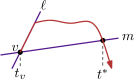
Figure 10: A central trajectory does not visit the half-line $\ell^{v\to}$.

∎

Corollary 21.

Let $\ell$ and $m$ be two positive increasing half-lines, of which $\ell$ is the steepest, and let $v$ be their intersection point. $\mathpzc{C}$ does not visit $\ell^{v\to}$, that is, $\ell^{v\to}\cap\mathpzc{C}=\emptyset$.

Consider two positive increasing half-lines $\ell$ and $\ell^{\prime}$ in $\mathcal{A}$, of which $\ell$ is the steepest, and let $v$ be their intersection point. Corollary 21 guarantees that $\mathpzc{C}$ never uses the half-line $\ell^{v\to}$. Hence, we can remove it from $\mathcal{A}$ (thus replacing $\ell$ by a line segment) without affecting $\mathpzc{C}$. By symmetry, it follows that we can clip one half-line from every pair of half-lines that are both increasing or decreasing. Let $\mathcal{A}^{\prime}$ be the arrangement that we obtain this way. See Fig. 11 for an illustration.

Figure 11: (a) The clipped increasing half-lines (purple) on top of the original half-lines (gray), and (b) the resulting arrangement $\mathcal{A}^{\prime}$ and its zone (in yellow).

Consider the set $\mathcal{Z}$ of open faces of $\mathcal{A}^{\prime}$ intersected by $\mathpzc{I}$, and let $E$ be the set of edges bounding them. We refer to $\mathcal{Z}\cup E$ as the zone of $\mathpzc{I}$ in $\mathcal{A}^{\prime}$.

Lemma 22.

$\mathpzc{C}$ is contained in the zone of $\mathpzc{I}$ in $\mathcal{A}^{\prime}$.

Proof. We can basically use the argument as in Lemma 20. Assume by contradiction that $\mathpzc{C}$ lies outside the zone from $u$ to $v$. The path from $u$ to $v$ along the border of the zone is $x$-monotone, hence there is a trajectoid $\mathpzc{T}$ that follows this path during $[t_{u},t_{v}]$ and for which $\mathpzc{T}(t)=\mathpzc{C}(t)$ at any other time. It follows that $\mathcal{D}^{\prime}(\mathpzc{T})<\mathcal{D}(\mathpzc{C})$ giving us a contradiction. ∎

Lemma 23.

The zone $\mathcal{Z}_{\ell}$ of a line $\ell$ in $\mathcal{A}^{\prime}$ has maximum complexity $8n$.

Proof. We show that the complexity of $\mathcal{Z}_{\ell}$ restricted to the positive half-plane is at most $4n$. A symmetric argument holds for the negative half-plane, thus proving the lemma. Since we restrict ourselves to the positive half-plane, the half-lines and segments of $\mathcal{A}^{\prime}$ correspond to two forests: a purple forest with $p$ segments, and a brown forest with $b$ segments. Furthermore, we have $p+b=n$.

Rotate all segments such that $\ell$ is horizontal. We now show that the number of left-bounding edges in $\mathcal{Z}_{\ell}$ is $2n$. Similarly, the number of right-bounding edges is also $2n$. Consider just the purple forest. Clearly, there are at most $p$ left-bounding edges in the zone of $\ell$ in the purple forest. We now iteratively add the edges of the brown forest in some order that maintains the following invariant: the already-inserted brown segments form a forest in which every tree is rooted at an unbounded segment (a half-line). We then show that every new left-bounding edge in the zone either replaces an old left-bounding edge or can be charged to a purple vertex or a brown segment. In total we gather $p+2b$ charges, giving us a total of $2p+2b=2n$ left bounding edges.

Let $s$ be a new brown leaf segment that we add to $\mathcal{A}^{\prime}$, and consider the set $J$ of all intersection points of $s$ with edges that form $\mathcal{Z}_{\ell}$ in the arrangement so far. The points in $J$ subdivide $s$ into subsegments $s_{1},..,s_{k}$ (See Fig. 12). All new edges in $\mathcal{Z}_{\ell}$ are subsegments of $s$. We charge the subsegment $s_{i}$ that intersects $\ell$ (if any), and $s_{k}$ to $s$ itself. The remaining subsegments replace either a brown edge or a purple vertex from $\mathcal{Z}_{\ell}$, or they yield no new left bounding edges. Clearly, segments replacing edges on $\mathcal{Z}_{\ell}$ do not increase the complexity of $\mathcal{Z}_{\ell}$. We charge the segments replacing purple vertices to those vertices. We claim that a vertex $v$ gets charged at most once. Indeed, each vertex has three incident edges, only two of which may intersect $\ell$. The vertex gets charged when a brown segment intersects those two edges between $v$ and $\ell$. After this, $v$ is no longer part of $\mathcal{Z}_{\ell}$ in that face (though it may still be in $\mathcal{Z}_{\ell}$ in its other faces). It follows that the total number of charges is $p+2b$.

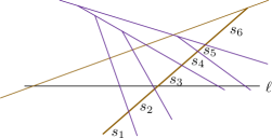
Figure 12: The new segment $s$ (fat) subdivided into subsegments. $s_{3}$ and $s_{6}$ are charged to $s$, $s_{5}$ is charged to a purple vertex. Segment $s_{4}$ replaces a purple edge in the zone, and $s_{1}$ and $s_{2}$ do not give new left bounding edges.

∎

Theorem 24.

Given $n$ lines, a trajectoid $\mathpzc{C}$ that minimizes $\mathcal{D}^{\prime}$ has worst case complexity $8n$.

Proof. $\mathpzc{C}$ is contained in the zone of $\mathcal{A}^{\prime}$. So the intersection vertices of $\mathpzc{C}$ are vertices in the zone of $\mathcal{A}^{\prime}$. By Lemma 23, the zone has at most $8n$ vertices, so $\mathpzc{C}$ has at most $8n$ vertices as well. ∎

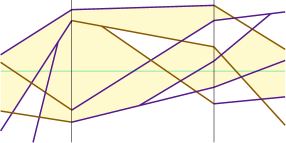
Figure 13: A piece of the zone in three consecutive slabs.

Let $\mathcal{A}^{*}$ be the total arrangement of all restricted functions; that is, a concatenation of the arrangements $\mathcal{A}^{\prime}$ restricted to the vertical slabs defined by their elementary time intervals. Define the global zone as the zone of $J$ in $\mathcal{A}^{*}$. Note that the global zone is more than just the union of the individual zones in the slabs, since cells can be connected along break points (and are not necesarily convex anymore). Nonetheless, we can still show that the complexity of the global zone is linear.

Lemma 25.

The global zone has complexity $24\tau n^{2}+48\tau n$.

Proof. The global zone is a subset of the union of the zones of $J$ and the vertical lines $x=t_{i}$, for $i\in{0,..,k}$ in the arrangements $\mathcal{A}^{\prime}$. By Lemma 23, a line intersecting a single slab has zone complexity $8n$. Each slab is bounded by two vertical lines and intersected by $J$, so applying the lemma three times yields a $24n$ upper bound on the complexity in a single slab. Since there are $\tau(n+2)$ elementary intervals, we conclude that the total complexity is at most $24\tau n^{2}+48\tau n$. ∎

As before, it follows that $\mathpzc{C}$ is in the zone of $\mathpzc{I}$ in $\mathcal{A}^{*}$. Thus, we conclude:

Theorem 26.

Given a set of $n$ trajectories in $\mathbb{R}^{1}$, each with vertices at times $t_{0},..,t_{\tau}$, a central trajectory $\mathpzc{C}$ with $\varepsilon=0$, has worst case complexity $O(\tau n^{2})$.

A.2 Algorithm

We now present an algorithm to compute a trajectoid $\mathpzc{C}$ minimizing $\mathcal{D}^{\prime}$. It follows from Lemma 2 that such a trajectoid is a central trajectory. The basic idea is to construct a weighted graph that represents a set of trajectoids, and is known to contain an optimal trajectoid. We then find $\mathpzc{C}$ by computing a minimum weight path in this graph.

The graph that we use is simply a weighted version of the global zone of $\mathpzc{I}$. We augment each edge $e=(u,v)$ in the global zone with a weight $\int_{t_{u}}^{t_{v}}|e(t)|\,\mathrm{d}t$. Hence, we obtain a weighted graph $\mathcal{G}$. Finally, we add one source vertex that we connect to the vertices at time $t_{0}$ with an edge of weight zero, and one target vertex that we connect with all vertices at time $t_{\tau}$. This graph represents a set of trajectoids, and contains an optimal trajectoid $\mathpzc{C}$.

We find $\mathpzc{C}$ by computing a minimum weight path from the source to the target vertex. All vertices except the source and target vertex have constant degree. Furthermore, all zones have linear complexity. It follows that $\mathcal{G}$ has $O(\tau n^{2})$ vertices and edges, and thus, if we have $\mathcal{G}$, we can compute $\mathpzc{C}$ in $O(\tau n^{2}\log(\tau n))$ time.

We compute $\mathcal{G}$ by computing the zone(s) of the arrangement $\mathcal{A}^{\prime}$ in each elementary interval. We can find the zone of $\mathcal{A}^{\prime}$ in $O((n+k)\alpha(n+k)\log n)=O(n\alpha(n)\log n)$ expected time, where $k$ is the complexity of $\mathpzc{C}$ and $\alpha$ is the inverse Ackermann function, using the algorithm of Har-Peled [17]. Since $\mathcal{A}^{\prime}$ has a special shape, we can improve on this slightly as follows.

We use a sweep line algorithm which sweeps $\mathcal{A}^{\prime}$ with a vertical line from left to right. We describe only computing the upper border of the zone (the part that lies above $\mathpzc{I}$). Computing the lower border is analogous. So in the following we consider only positive half-lines.

We maintain two balanced binary search trees as status structures. One storing all increasing half-lines, and one storing all decreasing half-lines. The binary search trees are ordered on increasing $y$-coordinate where the half-lines intersect the sweep line. We use a priority queue to store all events. We distinguish the following events: (i) a half-line starts or stops at $\mathpzc{I}$, (ii) an increasing (decreasing) half-line stops (starts) because it intersects an other increasing (decreasing) half-line, and (iii) we encounter an intersection vertex between an increasing half-line and a decreasing half-line that lies in the zone. In total there are $O(n)$ events.

The events of type (ii) involve only neighboring lines in the status structure, and the events of type (iii) involve the lowest increasing (decreasing) half-line and the decreasing (increasing) half-lines that are in the zone when they are intersected by the sweep line. To maintain the status structures and compute new events we need constantly many queries and updates to our status structures and event queue. Hence, each event can be handled in $O(\log n)$ time.

The events of type (i) are known initially. The first events of type (ii) and (iii) can be computed in $O(\log n)$ time per event (by inserting the half-lines in the status structures). So, initializing our status structures and event queue takes $O(n\log n)$ time. During the sweep we handle $O(n)$ events, each taking $O(\log n)$ time. Therefore, we can compute the zone of $\mathcal{A}^{\prime}$ in $O(n\log n)$ time in total.

Computing a minimum weight path

We can slightly improve the running time by reducing the time required to compute a minimum weight path. If, instead of a general graph $\mathcal{G}=(V,E)$ we have a directed acyclic graph (DAG), we can compute am minimum weight path in only $O(|V|+|E|)=O(\tau n^{2})$ time using dynamic programming. We transform $\mathcal{G}$ into a DAG by orienting all edges $e=(u,v)$, with $t_{u}<t_{v}$, from $u$ to $v$.

The running time is now dominated by constructing the graph. We conclude:

Theorem 27.

Given a set of $n$ trajectories in $\mathbb{R}^{1}$, each with vertices at times $t_{0},..,t_{\tau}$, we can compute a central trajectory $\mathpzc{C}$ for $\varepsilon=0$ in $O(\tau n^{2}\log n)$ time using $O(\tau n^{2})$ space.

References

- [1] P. K. Agarwal, M. de Berg, J. Gao, L. J. Guibas, and S. Har-Peled. Staying in the middle: Exact and approximate medians in and for moving points. In CCCG, pages 43–46, 2005.
- [2] P. K. Agarwal and M. Sharir. Arrangements and their applications. In J.-R. Sack and J. Urrutia, editors, Handbook of Computational Geometry, pages 49–119. Elsevier Science Publishers B.V. North-Holland, Amsterdam, 2000.
- [3] P. K. Agarwal and M. Sharir. Davenport-Schinzel sequences and their geometric applications. In J.-R. Sack and J. Urrutia, editors, Handbook of Computational Geometry, pages 1–47. Elsevier Science Publishers B.V. North-Holland, Amsterdam, 2000.
- [4] R. Basu, B. Bhattacharya, and T. Talukdar. The projection median of a set of points in . Discrete & Computational Geometry, 47(2):329–346, 2012.
- [5] M. Bern, D. Eppstein, P. Plassman, and F. Yao. Horizon theorems for lines and polygons. In J. Goodman, R. Pollack, and W. Steiger, editors, Discrete and Computational Geometry: Papers from the DIMACS Special Year, volume 6 of DIMACS Series in Discrete Mathematics and Theoretical Computer Science, pages 45–66. American Mathematical Society, Association for Computing Machinery, Providence, RI, 1991.
- [6] P. Bovet and S. Benhamou. Spatial analysis of animals’ movements using a correlated random walk model. J. Theoretical Biology, 131(4):419–433, 1988.
- [7] K. Buchin, M. Buchin, J. Gudmundsson, M. Löffler, and J. Luo. Detecting commuting patterns by clustering subtrajectories. International Journal of Computational Geometry & Applications, 21(03):253–282, 2011.
- [8] K. Buchin, M. Buchin, M. van Kreveld, M. Löffler, R. I. Silveira, C. Wenk, and L. Wiratma. Median trajectories. Algorithmica, 66(3):595–614, 2013.
- [9] K. Buchin, M. Buchin, M. van Kreveld, B. Speckmann, and F. Staals. Trajectory grouping structure. In Proc. 2013 WADS Algorithms and Data Structures Symposium, volume 8037 of LNCS, pages 219–230. Springer, 2013.
- [10] C. Calenge, S. Dray, and M. Royer-Carenzi. The concept of animals’ trajectories from a data analysis perspective. Ecological Informatics, 4(1):34 – 41, 2009.
- [11] E. D. Demaine, S. Eisenstat, L. J. Guibas, and A. Schulz. Kinetic minimum spanning circle. In Proceedings of the Fall Workshop on Computational Geometry, 2010.
- [12] S. Dodge, R. Weibel, and E. Forootan. Revealing the physics of movement: Comparing the similarity of movement characteristics of different types of moving objects. Computers, Environment and Urban Systems, 33(6):419–434, 2009.
- [13] S. Durocher and D. Kirkpatrick. The projection median of a set of points. Computational Geometry, 42(5):364 – 375, 2009.
- [14] S. Gaffney, A. Robertson, P. Smyth, S. Camargo, and M. Ghil. Probabilistic clustering of extratropical cyclones using regression mixture models. Climate Dynamics, 29(4):423–440, 2007.
- [15] S. Gaffney and P. Smyth. Trajectory clustering with mixtures of regression models. In Proc. 5th ACM SIGKDD Internat. Conf. Knowledge Discovery and Data Mining, pages 63–72, 1999.
- [16] E. Gurarie, R. D. Andrews, and K. L. Laidre. A novel method for identifying behavioural changes in animal movement data. Ecology Letters, 12(5):395–408, 2009.
- [17] S. Har-Peled. Taking a walk in a planar arrangement. SIAM Journal on Computing, 30(4):1341–1367, 2000.
- [18] S. Har-Peled and B. Raichel. The Fréchet distance revisited and extended. In Proc. of the Twenty-seventh Annual Symposium on Computational Geometry, SoCG ’11, pages 448–457, New York, NY, USA, 2011. ACM.
- [19] H. Imai and M. Iri. Polygonal approximations of a curve – formulations and algorithms. In Computational Morphology, pages 71–86. Elsevier Science, 1988.
- [20] J. Lee, J. Han, and K. Whang. Trajectory clustering: a partition-and-group framework. In Proc. ACM SIGMOD International Conference on Management of Data, pages 593–604, 2007.
- [21] X. Li, X. Li, D. Tang, and X. Xu. Deriving features of traffic flow around an intersection from trajectories of vehicles. In Proc. 18th International Conference on Geoinformatics, pages 1–5. IEEE, 2010.
- [22] J. Pach and P. K. Agarwal. Combinatorial Geometry. John Wiley & Sons, New York, NY, 1995.
- [23] B. Shneiderman. The eyes have it: a task by data type taxonomy for information visualizations. pages 336–343, 1996.
- [24] A. Stohl. Computation, accuracy and applications of trajectories – a review and bibliography. Atmospheric Environment, 32(6):947 – 966, 1998.
- [25] M. Vlachos, D. Gunopulos, and G. Kollios. Discovering similar multidimensional trajectories. In Proc. 18th Internat. Conf. Data Engineering, pages 673–684, 2002.