Radio jet emission from GeV-emitting narrow-line Seyfert 1 galaxies

Abstract

Context. With the current study we aim at understanding the properties of radio emission and the assumed jet from four radio-loud and $\gamma$-ray-loud narrow-line Seyfert 1 galaxies. These are Seyfert 1 galaxies with emission lines at the low end of the FWHM distribution.

Aims. The ultimate goal is twofold: first we investigate whether a relativistic jet is operating at the source producing the radio output, and second, we quantify the jet characteristics to understand possible similarities with and differences from the jets found in typical blazars.

Methods. We relied on the most systematic monitoring of radio-loud and $\gamma$-ray-detected narrow-line Seyfert 1 galaxies in the cm and mm radio bands conducted with the Effelsberg 100 m and IRAM 30 m telescopes. It covers the longest time-baselines and the most radio frequencies to date. This dataset of multi-wavelength, long-term radio light-curves was analysed from several perspectives. We developed a novel algorithm to extract sensible variability parameters (mainly amplitudes and time scales) that were then used to compute variability brightness temperatures and the corresponding Doppler factors. The jet powers were computed from the light curves to estimate the energy output and compare it with that of typical blazars. The dynamics of radio spectra energy distributions were examined to understand the mechanism causing the variability.

Results. The length of the available light curves for three of the four sources in the sample allowed a firm understanding of the general behaviour of the sources. They all display intensive variability that appears to be occurring at a pace rather faster than what is commonly seen in blazars. The flaring events become progressively more prominent as the frequency increases and show intensive spectral evolution that is indicative of shock evolution. The variability brightness temperatures and the associated Doppler factors are moderate, implying a mildly relativistic jet. The computed jet powers show very energetic flows. The radio polarisation in one case clearly implies a quiescent jet underlying recursive flaring activity. Finally, in one case, the sudden disappearance of a $\gamma$-ray flare below some critical frequency in our band needs a more detailed investigation of the possible mechanism causing the evolution of broadband events.

Conclusions. Despite the generally lower flux densities, the sources appear to show all typical characteristics seen in blazars that are powered by relativistic jets, such as intensive variability, spectral evolution across the different bands following evolutionary paths explained by travelling shocks, and Doppler factors indicating mildly relativistic speeds.

1 Introduction

Seyfert galaxies were first identified as a distinct class of extragalactic systems by Seyfert (1943), who studied the nuclear emission of six “extragalactic nebulae” with “high excitation nuclear emission lines superposed on a normal G-type spectrum”. The lines appeared to be broadened, reaching widths of about 8500 km s^-1. Seyfert also noted that the maximum width of the Balmer emission lines increased with the luminosity of the nucleus as well as the ratio between the light from the nucleus and the total light of the object, setting the scene for the class of Seyfert galaxies that in summary show, bright, star-like nucleus, and broad emission lines that cover a wide range of ionisation states. Khachikian & Weedman (1974) much later classified Seyfert galaxies into types 1 and 2 depending on whether the H$\beta$ lines (Balmer series) are broader than the forbidden ones, or of approximately the same width. Typically, the width of forbidden lines in both classes are of the order of “narrow emission lines”, that is, of about 300–800 km s^-1, while the width of “broad emission lines” – including the hydrogen Balmer lines – is about 1000–6000 km s^-1 (Osterbrock, 1984).

Davidson & Kinman (1978) found that MRK 359 appeared, to be lying at the low end of the line-width distribution and to have H$\beta$ and forbidden lines of comparable widths that were similar to those in Seyfert 2 galaxies ($\approx 300$ km s^-1); furthermore, MRK 359 showed strong featureless continuum, and strong high-ionisation lines (e.g. [Fe vii] and [Fe x]); these properties are common in Seyfert 1 galaxies, which led to the definition of yet another sub-class of AGN: the “narrow-line Seyfert 1” – hereafter NLSy1 – galaxies (Gaskell, 1984; Osterbrock & Pogge, 1985; Osterbrock & Dahari, 1983). Koski (1978) and Phillips (1978) noted that MRK 42 showed a similar behaviour. Osterbrock & Pogge (1985) studied eight such sources and concluded that they are characterised by (a) unusually narrow H$\beta$ lines, (b) strong Fe ii emission, (c) normal luminosities, and (d) H$\beta$ slightly weaker than in typical Seyfert 1 galaxies. Conventionally, today sources are categorised as NLSy1 if they show (a) a narrow width of the broad Balmer emission line with a FWHM(H$\beta$) $\lesssim 2000$ km s^-1, and (b) weak forbidden lines with [O iii]$\lambda$5007/H$\beta$ $<$ 3 (Osterbrock & Pogge, 1985; Goodrich, 1989; Zhou et al., 2006).

The first attempts to investigate the radio properties of these systems were undertaken by Ulvestad et al. (1995), among others, who studied seven NLSy1s with the Very Long Array (VLA) in A configuration at 5 GHz. They found that the radio power was moderate ($10^{20-23}$ W Hz^-1), the emission is compact ($<300$ pc), and in the two of three cases where radio axes could be found and high optical polarisation was detected, the radio axes were oriented perpendicularly to the electric vector position Angle (EVPA); the third one showed EVPA nearly parallel to the radio axis. Later, Moran (2000) also studied 24 NLSy1s with the VLA in A configuration to confirm that most of the sources were unresolved and that they showed relatively steep spectra. Stepanian et al. (2003) investigated 26 NLSy1 galaxies and found that only 9 were detected in the FIRST catalogue (White et al., 1997), and all were radio-quiet. Komossa et al. (2006) studied 128 NLSy1s in a dedicated search for radio-loud (RL) NLSy1s and concluded, among others, that (a) their morphology is similar to compact steep-spectrum sources (CSS; Gallo et al., 2006, discussed PKS 2004$-$447 as an example of NLSy1 that was also CSS); (b) the radio-loudness $R$ – defined as the ratio of the 6 cm flux to the optical flux at 4400 $\AA$ (Kellermann et al., 1989) – is distributed smoothly up to the critical value of 10 and covers about four orders of magnitude; (c) almost 7 % of the NLSy1 galaxies are formally RL, but only 2.5 % of them exceed a radio index $R>100$; (d) most RL NLSy1 are compact steep-spectrum sources, than accreting close to or above the Eddington luminosity, $L_{\mathrm{Edd}}$; (e) the black-hole masses are generally at the upper observed end for NLSy1, but are still smaller than what is typically seen in other RL AGNs.

Even before the detection of the RL subset of this class at high energies, it was clear that they comprise a special source type for a number of reasons. Yuan et al. (2008) studied a sample of 23 NLSy1s with a radio-loudness exceeding 100 to find that these RL AGNs may be powered by black holes of moderate masses ($10^{6}$–$10^{7}$ M_☉) accreting at high rates and that they show a variety of radio properties reminiscent of blazars. Komossa et al. (2006) pointed out that NLSy1s provide an excellent probe for studying the physics scaling towards lower black-hole masses given their systematically low black-hole masses in the range $10^{6}$–$10^{8}$ M_⊙. Despite the fundamental differences between RL NLSy1s and blazars – in terms of black-hole masses and accretion disc luminosities ($0.2$–$0.9$ $L_{\mathrm{Edd}}$) – their jets seem to be behaving similarly and share the same properties (see also Foschini, 2012b). That alone has implications on the energy production and dissipation at different scales.

According to Komossa et al. (2006), an important question arising from the behaviour of these systems is whether or not the black-hole mass and radio-loudness are related and especially whether there is a limiting black-hole mass above which objects are preferentially RL, and whether or not RL and radio-quiet galaxies show the same spread in their black-hole masses. On this ground, Komossa (2008) argued that the study of NLSy1s needs to (a) include the radio and infrared properties of NLSy1 galaxies when correlation analyses are performed, (b) determine the sufficient and necessary conditions for the onset of NLSy1 activity, and (c) the investigation of whether the low black-hole mass is enough to explain the typically observed NLSy1 characteristics.

The first report for the detection of $\gamma$-ray emission from a source classified as an RL NLSy1 was given by Abdo et al. (2009a) and Foschini et al. (2010), who discussed the detection of significant GeV emission by the Fermi/LAT instrument from PMN J0948$+$0022. Already in its first year of operations, Fermi/LAT detected a total of four NLSy1s (Abdo et al., 2009c). As of today, there are seven RL NLSy1s detected in the MeV–GeV energy bands five of which with high significance (TS$>25$, see also D’Ammando et al., 2013b; Foschini et al., 2014). A thorough review of the recent discoveries is given by Foschini (2012b).

The multi-wavelength campaigns that followed these discoveries (e.g. Abdo et al., 2009b, a; Giroletti et al., 2011; Foschini et al., 2012; Fuhrmann et al., 2011) and the study of subsequently discovered NLSy1s (Abdo et al., 2009c) showed a clear blazar-like behaviour, indicating the existence of a relativistic jet viewed at small angles.

Despite the research activity that their high-energy detection has motivated, several questions remain open. Especially the exact nature and properties of NLSy1s and the properties of the jet that seems to be present. Particularly in the radio regime, where a jet is expected to be dominant, the studies conducted so far have mostly been based on non-simultaneous datasets.

In the current work we quantify some of the properties of the assumed radio jet emission. The motivation for this is to compare them with those seen in other classes of AGNs – especially blazars. To do this, we studied the radio behaviour of four RL NLSy1s detected in $\gamma$ rays by Fermi/LAT through regular multi-band, single-dish radio monitoring with the Effelsberg 100 m and IRAM 30 m telescopes. We focus on the variability properties – especially brightness temperatures and variability Doppler factors, which will (in a later publication) be combined with long-baseline radio interferometric measurements to estimate the viewing angles and Lorentz factors (Fuhrmann et al., in prep.). The energetics of the observed radio outbursts and the variability patterns of the broadband radio spectra are seen as indicators of the variability and emission mechanism at play. Very early results have been presented in several other studies, including D’Ammando et al. (2012), Fuhrmann et al. (2011), and Foschini et al. (2012).

Here we present the longest-term, multi-frequency radio monitoring datasets of the known $\gamma$-ray-detected and radio-loud NLSy1s to date. As an example, the 4.85 GHz light-curve lengths, range between longer than 1.5 years and longer than 5 years. The monitoring was conducted at eight different frequencies for the two brightest sources and at six frequencies for the faintest.

The paper is structured as follows: in Sect. 2 we review some archival information about the sources in our sample that is necessary for the following discussion. After describing the observing methods in Sect. 3, we continue in Sect. 4 with the phenomenological description of the obtained light curves. The light curves discussed there comprise the basis for the flare decomposition method presented in Sect. 5. Subsequently, we continue in the frequency domain by studying the radio spectra in Sect. 6. In Sect. 7 we compute the radio powers for the 14.60 GHz datasets, while in Sect. 8 we discuss our polarisation measurements. Summarising comments are discussed in Sect. 8, where we describe the general connection of all our findings. The main findings of our study are presented in Sect. 10, which concludes the paper.

Throughout the paper we assume a $\Lambda CDM$ cosmology with $H_{0}=70$ km s^-1 Mpc^-1 and $\Omega_{\Lambda}=0.73$ (Komatsu et al., 2011).

2 The sample: what is already known

Table 1: The four monitored NLSy1s with their observed positions, redshift, and classification.

Source ID	Survey name	RA	DEC	z	Class
		(hh:mm:ss.s)	(dd:mm:ss.s)
J0324$+$3410	B2 0321+33B	03:24:41.2	$+$34:10:45.1	0.0610a	NLSy11
				0.0629b
J0849$+$5108	SBS 0846$+$513	08:49:58.0	$+$51:08:29.0	0.584701c	NLSy12
J0948$+$0022	PMN J0948$+$0022	09:48:57.3	$+$00:22:25.6	0.585102c	NLSy13
J1505$+$0326	PKS 1502$+$036	15:05:06.5	$+$03:26:31.0	0.407882c	NLSy14

(a) Marcha et al. (1996); (b) Zhou et al. (2007); (c) Marcha et al. (1996); (1) Zhou et al. (2007); (2) Greene & Ho (2005); (3) Zhou et al. (2003); (4) Zhou et al. (2006)

We here investigate a sample of four sources, which are

1. classified as NLSy1s,

2. radio-loud,

3. detected at $\gamma$ rays by the Fermi/LAT, and

4. satisfy certain observational constrains such as declination limits and a sufficiently high flux density to enable quality measurements at the Effelsberg ($\gtrsim 0.1$ Jy) and IRAM telescopes ($\gtrsim 0.3$ Jy).

We briefly summarise what is already known of these sources. Table 1 summarises their positions, redshifts, and classifications.

2.1 J0324$+$3410 (1H 0323$+$342)

The source J0324$+$3410 is of special interest mostly because of the morphology of its host galaxy and the estimated black-hole mass. From two HST archival images (each of 200 s exposure), Zhou et al. (2007) concluded that it is hosted by a one-armed spiral galaxy. The authors showed that its radio and X-ray emission can be explained by jet synchrotron radiation, while the infrared and optical light is dominated by thermal emission from a Seyfert nucleus. Antón et al. (2008) conducted $B$- and $R$-band observations with the Nordic Optical Telescope (NOT). They suggested that its host resembles the morphology seen in the inner parts of Arp 10 found by Charmandaris & Appleton (1996), implying that J0324$+$3410 may be a merger remnant. Following the method discussed by Greene & Ho (2005), they estimated the central black-hole mass to be $10^{7}\leavevmode\nobreak\ \mathrm{M}_{\sun}$; this value lies in the overlapping region between the black-hole mass distributions for NLSy1s and blazars and is similar to the value published earlier by Zhou et al. (2007).

Although the only case of an RL, Fermi-detected NLSy1 for which the host is well resolved, J0324$+$3410, challenges the assumptions that powerful relativistic jets form only in giant elliptical galaxies (e.g. Böttcher & Dermer, 2002; Sikora et al., 2007).

Abdo et al. (2009c) presented a thorough study including spectral energy distribution (hereafter SED) fits. The presence of a jet was already apparent in these studies; but in an episodic manner and not as a fully developed constantly broadband-emitting jet. The computed jet power placed the source in the BL Lac range (see jet power computations in Sect. 7). It is worth noting that they computed accretion rates that reach extreme values of up to 90 % of the Eddington luminosity, yet another peculiar property of the RL, $\gamma$-ray-loud NLSy1s.

2.2 J0849$+$5108 (SBS 0846$+$513)

J0849$+$5108 was identified as an NLSy1 galaxy by Zhou et al. (2005). They found clear evidence for emission from a relativistic jet and a stellar component. Additionally, the emission lines show characteristics that classify it as a typical NLSy1 (FWHM(H$\beta$)$\simeq 1710$ km s^-1, [O iii]$\lambda_{5007}\simeq 0.32\ \mathrm{H}\beta$ and strong Fe ii emission). The fact that the source was previously classified as a BL Lac object (Arp et al., 1979) makes the case especially interesting, possibly providing a handle on the link between BL Lac objects and NLSy1s.

Yuan et al. (2008) included the source in a very thorough study of a sample of 23 RL NLSy1 galaxies and reported a black-hole mass of about $10^{7.4}$ M_☉. On the basis of the detected significant optical polarisation, they claimed that it has a jet. Finally, they found that during the high-energy states the optical continuum is featureless, while at low states strong emission lines become obvious; this suggests that the source maybe a transition between a quasar and a BL Lac that displays its latter character only at flaring states.

Foschini (2011b) was the first to report its detection at $\gamma$ rays. Later, D’Ammando et al. (2012) discussed a flaring episode around June–July 2011. The multi-frequency datasets collected during the campaigns following the detection are partly discussed in D’Ammando et al. (2013c). Using the Very Long Baseline Array (VLBA) at 5, 8.4 and 15 GHz D’Ammando et al. (2012) resolved the otherwise compact source to reveal a core-jet structure. The feature attributed to the jet shows a steep spectrum. The core has been decomposed into two compact components. They discussed the detection of an apparent speed of about 8 c, indicating a relativistic jet. In summary, the power output (isotropic $\gamma$-ray luminosity) of $10^{48}$ erg s^-1 on a daily scale (similar to that of luminous flat-spectrum radio quasars, FSRQs), the apparent superluminal motions and the radio variability accompanied by spectral evolution indicate blazar-like relativistic jet.

D’Ammando et al. (2012) also considered the suggestion of Ghisellini & Tavecchio (2008) and Ghisellini et al. (2011) that the transition between FSRQs and BL Lac can be interpreted in terms of different accretion rates. They found that the position of the source in a $\gamma$-ray photon index against luminosity plot ($\Gamma_{\mathrm{\gamma}}-L_{\mathrm{\gamma}}$) also places it in the typical blazar territory.

2.3 J0948$+$0022 (PMN J0948$+$0022)

J0948$+$0022 shows the usual characteristics of an NLSy1 optical spectrum (Williams et al., 2002) with a FWHM(H$\beta$) of 1500$\pm$55 km s^-1, O iii/H$\beta<3$, and strong optical F ii emission (Zhou et al., 2003). Although NLSy1s are usually radio quiet (e.g. Ulvestad et al., 1995; Komossa et al., 2006), J0948$+$0022 was found to be the first very radio-loud NLSy1 with a $R>10^{3}$ (Zhou et al., 2003). In addition, Zhou et al. (2003) reported an inverted radio spectrum and high brightness temperatures, which strongly supports that there is a relativistic, Doppler-boosted jet seen at small viewing angles. The source has also been the first NLSy1 detected at high-energy $\gamma$ rays by Fermi/LAT during its first months of operation. Fermi/LAT confirmed the relativistic jet emission from this source and established NLSy1s as a new class of $\gamma$-ray emitting AGNs (Foschini et al., 2010; Abdo et al., 2009a, b).

At pc scales, the source appears as one-sided VLBI structure dominated by a compact ($<55$ $\mu$as), bright central component (Doi et al., 2006; Giroletti et al., 2011). Kpc-scale radio emission has also been found by Doi et al. (2012) with a two-sided extension of the core and a northern extent of 52 kpc in projected distance. From these studies a relativistically boosted jet with Doppler factors $D>1$ (e.g. $D>2.7-5.5$ Doi et al., 2006) has been inferred, in agreement with Doppler boosting inferred from previous variability studies (e.g. Fuhrmann et al., 2011).

This NLSy1 is variable across the whole electromagnetic spectrum. Intense multi-wavelength campaigns performed over the past years revealed continuous activity with an exceptional outburst in 2010 (Foschini et al., 2011) that occurred at all spectral bands. Together with detailed SED modelling and the detection of polarised emission, these findings confirm the powerful relativistic jet in the source seen at small viewing angles.

2.4 J1505$+$0326 (PKS 1502$+$036)

Based on its optical characteristics (FWHM(H$\beta)=1082\pm 113$ km s^-1, [O iii]/H$\beta$$\sim 1.1$, and a strong optical Fe ii bump), this source was classified as NLSy1 (e.g. Yuan et al., 2008). It exhibits one of the highest radio-loudness parameters among NLSy1s ($R=1549$, see also Sect. 2.5). Early VLBI observations revealed a compact source (marginally resolved at milli-arcsecond scales) with an inverted radio spectral index (Dallacasa et al., 1998).

Abdo et al. (2009c) reported the first detection of $\gamma$-ray emission from the source by Fermi/LAT. From SED modelling the authors inferred jet powers similar to those in J0948$+$0022 and those typically observed in powerful quasars. A detailed multi-wavelength campaign carried out between 2008 and 2012 did not reveal any significant variability at $\gamma$ rays, in contrast to prominent flux density and spectral variability seen in the radio regime (D’Ammando et al., 2013a). The 15 GHz VLBI imaging showed a one-sided core-jet structure on pc scales. No significant proper motion of jet components was detected. The radio variability and VLBI findings together with an inferred high apparent isotropic $\gamma$-ray luminosity strongly support a relativistic, Doppler-boosted jet in this case as well.

2.5 Radio-loudness

Of the four sources in our study, J0948$+$0022, J0849$+$5108, and J1505$+$0326 are very RL, with $R_{1.4}=194-793$ (Komossa et al., 2006),1445 and 1549 (Yuan et al., 2008), respectively; where $R$ is the radio index according to Kellermann et al. (1989). J0324$+$3410 is only mildly RL with $R_{5}=38-71$ (Zhou et al., 2007). We note that each value of $R$ is uncertain by a factor of a few to 10, reflecting uncertainties in extinction correction, optical host contribution, and variability in the radio or optical bands. The monitoring presented here, reveals variability in the radio bands of up to several ten of percent (see Table 8), but not high enough to modify the previous source classification as RL or radio-quiet. The values of the radio indices reported in the literature are therefore adequate for the scope of this paper and are shown in Table 2.

Table 2: Radio-loudness of the sources in our sample. The moderate variability cannot cause remarkable changes in the $R$ indices, making the published values representative enough.

Source	Radio Index	Reference
J0324$+$3410	$R_{5}=38-71$	(1) based on HST optical flux
J0948$+$0022	$R_{1.4}=194-793$	(2) based on USNO and GSC catalogues (note the variable optical flux)
J0849$+$5108	$R_{1.4}=1445$	(3) based on SDSS optical flux
J1505$+$0326	$R_{1.4}=1549$	(3) …

(1) Zhou et al. (2007); (2) Komossa et al. (2006); (3) Yuan et al. (2008).

3 Observations and data reduction

The light curves and radio SEDs presented here have been observed in the framework of the F-GAMMA programme (Fuhrmann et al., 2007; Angelakis et al., 2010). They cover the frequency range from 2.64 to 142.33 GHz. Below 43.05 GHz the measurements were conducted with eight different heterodyne receivers mounted on the secondary focus of the 100 m Effelsberg telescope. The observations at 86.24 and 142.33 GHz were obtained with the 30 m IRAM telescope. In Table 4 their most important operational characteristics are summarised .

3.1 Effelsberg observations

The Effelsberg station covers the band between 2.64 and 43.05 GHz. The systems at 4.85, 10.45 and 32 GHz are equipped with multiple feeds allowing differential measurements meant to remove atmospheric effects (e.g. emission or absorption fluctuations). The rest are equipped with only single feeds. All receivers have circularly polarised feeds. The observations are made in cross-scanning mode, that is monitoring the telescope response while driving over the source position in two different orthogonal directions (in our case, azimuth and elevation). Necessary post-measurement corrections include the following:

1. Pointing-offset correction: meant to correct for the power loss caused by possible divergence of the actual source position from that observed by the telescope. This effect is of the order of a few percent.

2. Atmospheric-opacity correction: meant to correct for the attenuation caused by the transmission through the terrestrial atmosphere. This effect can be significant especially at higher frequencies where the atmospheric opacity becomes significantly high.

3. Elevation-dependent gain correction: correcting for sensitivity losses caused by small-scale departures of the primary reflector’s geometry from that of an ideal paraboloid (as expected for a homology-designed reflector). The magnitude of this effect is constrained to within a few percent.

4. Absolute calibration: converting the measured antenna temperatures to SI units by reference to standard candles, that is, calibrators. The standard candles used for our programme along with the flux densities assumed for them are shown in Table 3. Specifically, in the case of NGC 7027, a partial power loss caused by its extended structure relative to the beam size above 10.45 GHz was corrected for.

   Table 3: Flux densities of the standard calibrators used at Effelsberg.

   Source:	3C 48	3C 161	3C 286	3C 295	NGC 7027
   $S_{2.64}$	9.51	11.35	10.69	12.46	3.75
   $S_{4.85}$	5.48	6.62	7.48	6.56	5.48
   $S_{8.35}$	3.25	3.88	5.22	3.47	5.92
   $S_{10.45}$	2.60	3.06	4.45	2.62	5.92
   $S_{14.60}$	1.85	2.12	3.47	1.69	5.85
   $S_{23.05}$	1.14	1.25	2.40	0.89	5.65
   $S_{32.00}$	0.80	0.83	1.82	0.55	5.49
   $S_{43.00}$	0.57	0.57	1.40	0.35	5.34

   The flux densities of the calibrators are taken from Ott et al. (1994), Baars et al. (1977), Zijlstra et al. (2008), and Kraus priv. comm.

The five-year mean magnitudes of these effects as they are observed by the F-GAMMA programme are summarised in Table 5.

3.2 IRAM observations

Observations with the IRAM 30 m telescope were made within the F-GAMMA monitoring programme and the more general flux monitoring conducted by IRAM (Institut de Radioastronomie Millimétrique, Ungerechts et al., 1998). Data from both programmes are included in this paper. The observations were conducted with the newly installed EMIR receiver (Carter et al., 2012) using the 3 and 2 mm bands (each with linear polarisation feeds) tuned to 86.24 and 142.33 GHz and the narrow-band continuum backends (1 GHz bandwidth) attached. Observations of J0324$+$3410 and J0948$+$0022 were performed with cross-scans in azimuth and elevation direction and wobbler-switching along azimuth with a frequency near 2 Hz. Each cross-scan was preceded by a calibration scan to obtain instantaneous opacity information (e.g. Mauersberger et al., 1989). After data quality control, the sub-scans of each scanning direction were averaged and fitted with Gaussian curves. In the next step, each amplitude was corrected for small remaining pointing offsets and systematic gain-elevation effects. This operation has an effect of about 1 % at 86.24 GHz and 4 % at 142.33 GHz (mean pointing offsets are 1.8 ″for both receivers). The latter correction, and given the IRAM 30 m elevation-dependent gain curves, amounts to $\lesssim 5$ %. The conversion to the standard flux density scale was made using frequent observations of primary (Mars, Uranus) and secondary (W3OH, K3-50A, NGC 7027) calibrators.

Table 4: Receiver characteristics.

$\nu$	$\lambda$	$\Delta\nu$	$T_{\mathrm{sys}}$	$FWHM$	Feeds	Polarisation	Aperture Efficiency
(GHz)	(mm)	(GHz)	(K)	(″)			(%)
2.64	110	0.1	17	260	1	LCP, RCP	58
4.85	60	0.5	27	146	2	LCP, RCP	53
8.35	36	1.2	22	82	1	LCP, RCP	45
10.45	28	0.3	52	68	4	LCP, RCP	47
14.60	20	2.0	50	50	1	LCP, RCP	43
23.05	13	2.7	77	36	1	…	30
32.00	9	4.0	64	25	7	LCP	32
43.05	7	2.8	120	20	1	…	19
86.24	3	8.0 (1 GHZ used)	$\sim$65	29	1	HLP, VLP	63
142.33	2	4.0 (1 GHZ used)	$\sim$65	16	1	HLP, VLP	57

Table 5: The average fractional effect of each post-measurement correction applied to the data for each observing frequency. The numbers represent the 5-year average behaviour as it is observed by the F-GAMMA programme.

Frequency	Pointing	Opacity	Gain
	Correction	Correction	Correction
(GHz)	(%)	(%)	(%)
Effelsberg
2.64	0.5	2.3	0.0
4.85	0.4	2.5	1.2
8.35	0.5	2.5	0.9
10.45	1.2	3.1	1.2
14.60	1.3	2.9	1.3
23.05	1.6	8.1	2.1
32.00	3.1	7.9	2.9
43.05	5.1	20.	2.1
IRAM
86.24	1.0	…	5.0
142.33	4.0	…	5.0

3.3 Error estimates

In every operational step the errors were propagated formally assuming Gaussianity. The exact details are discussed in separate papers (Nestoras et al. in prep., for the IRAM observations; Angelakis et al. in prep., for the Effelsberg observations). An indicative empirical measure of the uncertainty in a measurement can be given by the fractional fluctuations seen in sources known to be intrinsically stable, that is to say, the calibrators. The datasets available for these sources cover the entire period of observations and include – cumulatively – all possible sources of fluctuations. This variability – seen in sources intrinsically stable – must also be present in the light curves of the targets. In Table 6 we quote the mean flux density at each frequency for each calibrator used at Effelsberg and NGC 7027 used at IRAM. Note that the flux density for each such source was computed using the mean calibration factor of each session. There we also show the modulation index defined as $m=100\cdot\frac{\sigma}{\left<S\right>}$ with $\sigma$ being the standard deviation and $\left<S\right>$ the mean flux density. $m$ remains at levels of a few percent even at frequencies above 23.05 GHz where the troposphere becomes very disturbing.

Table 6: The mean flux density and modulation index of the calibrators at each frequency.

Source	Observable	Units	2.64	4.85	8.35	10.45	14.60	23.05	32.00	43.05	86.24	142.33
3C 286	N		102	108	108	111	106	101	89	46	…	…
	$\left<S\right>$	(Jy)	10.710	7.477	5.2189	4.453	3.476	2.408	1.840	1.429	…	…
	$m$	(%)	0.9	0.5	0.7	1.1	1.9	2.9	3.5	4.4	…	…
3C 48	N		88	91	92	92	93	83	72	28	…	…
	$\left<S\right>$	(Jy)	9.579	5.509	3.267	2.613	1.872	1.162	0.817	0.599	…	…
	$m$	(%)	0.7	0.6	0.9	1.2	1.7	2.9	4.6	4.5	…	…
3C 161	N		30	35	29	30	30	22	19	4	…	…
	$\left<S\right>$	(Jy)	11.361	6.597	3.793	2.961	2.053	1.221	0.822	0.597	…	…
	$m$	(%)	1.0	0.8	1.4	2.2	3.3	5.4	7.3	2.3	…	…
3C 295	N		38	38	34	35	35	25	24	…	…	…
	$\left<S\right>$	(Jy)	12.499	6.546	3.434	2.588	1.690	0.880	0.557	…	…	…
	$m$	(%)	0.9	0.8	1.3	1.5	2.6	6.4	6.7	…	…	…
NGC7027	N		64	73	79	75	71	62	52	25	61	54
	$\left<S\right>$	(Jy)	3.693	5.449	5.903	5.912	5.738	5.455	5.243	5.146	4.920	4.611
	$m$	(%)	1.2	0.5	1.1	1.2	2.1	3.8	5.3	5.3	2.7	4.6

3.4 Cross-telescope calibration

Because below we discuss the dynamics of radio SEDs observed partly with the Effelsberg and partly with the IRAM 30 m telescope, it is essential to address the cross-telescope calibration accuracy that might introduce artefacts in the observed spectral shapes and their apparent temporal behaviour. An empirical yet reliable measure of its goodness can be provided by NGC 7027, which exhibits a flux density high enough to be detected by both instruments with high signal-to-noise ratios (S/N) and repeatedly. NGC 7027 has a very well defined and analytically described time-dependent convex spectrum (Zijlstra et al., 2008) that at frequencies above roughly $\sim 10$ GHz can be approximated by a power law of the form $S\propto\nu^{-0.1}$. In Fig. 1 we show the flux densities averaged over the entire period discussed here and for all frequencies. Each circle denotes an average flux density. The red symbols (with $\nu\geq 10.45$ GHz) are the Effelsberg measurements that were used for the model fit, and the red line is the result of the fit. The grey area is confined by 1$\sigma$ of each average flux density. Extrapolating the fitted spectrum (red dotted-dashed line) towards the higher IRAM band and comparing these values with the measured IRAM 30 m flux densities yields differences better than 3 %, specifically, 2.7 % at 86.22 GHz and 2.8 % at 142.33 GHz), indicating a high-quality cross-telescope calibration.

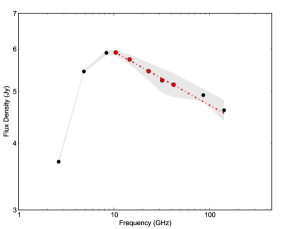
Figure 1: Observed radio SED of NGC 7027 (Zijlstra et al., 2008) over the same period of time as the time baseline covered here. All the Effelsberg frequencies from 2.64 up to the highest IRAM frequency of 142.33 GHz are shown. The filled circles (red and black) denote the measurements. The red symbols mark the Effelsberg measurements that where used in the fit, the red dotted-dashed line is the fitted spectrum. The grey area denotes the 1$\sigma$ region around each data point. The agreement of the extrapolated values with those measured by IRAM is better than 3 %.

3.5 Analysis methods

The current section introduces notions and methods that are used below, even if they are repeated briefly in the corresponding sections.

Internal shocks causing variability:

One of the aims here is to study the mechanism that may be causing the observed variability. Throughout the text it is assumed that this could well be caused by internal shocks that propagate in the jet, imprinting a specific signature in the radio light curves. In this model (Marscher & Gear, 1985; Türler et al., 2000), the synchrotron self-absorbed component is undergoing distinct evolutionary stages, each characterised by a different energy-loss mechanism. The followed path then imprints a distinct phenomenology on the radio SEDs, making this model easily quantifiable and testable. It has been argued that the implementation of this scenario in a system with simply a steep-spectrum quiescent jet is enough to reproduce the observed plurality of phenomenologies (Angelakis et al., 2012b).

The variability brightness temperature:

As discussed extensively in Sect. 5, the variability brightness temperature is a measure of the energetics of the associated event. It is computed on the basis of the light travel-time argument and depends on the magnitude of the flux density variation, $\delta S$ and the time span needed for that variation, $\delta t$. The flare decomposition method (Sect. 5) aims at separately estimating exactly those parameters for each event. The variability brightness temperature at the source rest frame in K, is given by

$$T_{\mathrm{var}}=1.64\cdot 10^{10}\cdot\frac{\delta S\cdot d^{2}_{\mathrm{L}}\cdot\lambda^{2}}{{\delta t}^{2}\cdot(1+z)^{4}},$$

where

$$\begin{array}[]{lp{0.8\linewidth}}\delta S&is the increase in flux density (at the observer's frame) in units of Jy,\\ \delta t&is the time span needed for that increase (at the observer's frame) in units of days,\\ d_{\mathrm{L}}&is the source luminosity distance in units of Mpc,\\ \lambda&is the observing wavelength in units of cm, and\\ z&is the source redshift,\end{array}$$

all measured at the observer’s frame.

Any excess from an independently computed intrinsic limit is then interpreted in terms of the Doppler-boosting factor $D$ as

$$D=(1+z)\sqrt[3+\alpha]{\frac{T_{\mathrm{var}}}{T_{\mathrm{ref}}}},$$ (1)

where

$$\begin{array}[]{lp{0.8\linewidth}}\alpha&is the source spectral index with $S\propto\nu^{\alpha}$,\\ T_{\mathrm{ref}}&is the limiting value of the brightness temperature.\end{array}$$

The value for the spectral index in the previous equation is chosen to be the mean values in the corresponding sub-band as given in Table 10. In Sect. 5 we explain that the limiting value is based on the equipartition argument as proposed by Readhead (1994).

4 Radio light curves

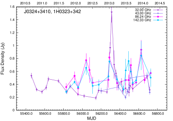
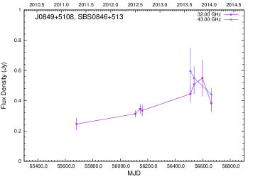
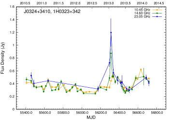
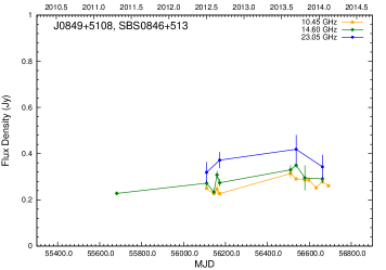
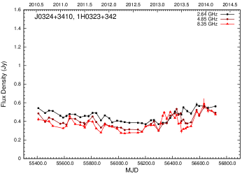
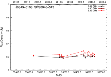
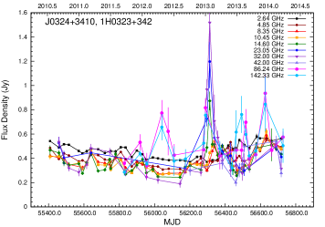
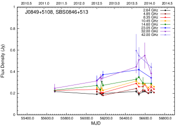
Figure 2: Radio light curves available for J0324$+$3410 (left column) and J0849$+$5108 (right column) at all available frequencies. From top to bottom we present the light curves three different frequency bands: low: 2.64, 4.85 and 8.35 GHz, intermediate: 10.45, 14.60 and 23.05 GHz, and high: 32, 43.05, 86.24 (when available) and 142.33 GHz (when available). At the very bottom the datasets are shown over-plotted together for comparison. For the same reason, for each source and axes the boundaries are kept identical. Lines connecting the data points have been used everywhere to facilitate visual inspection. Each frequency is consistently represented by the same colour and symbol. Only data points with a signal-to-noise ratio better than 3 have been used.

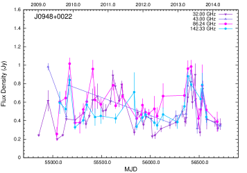
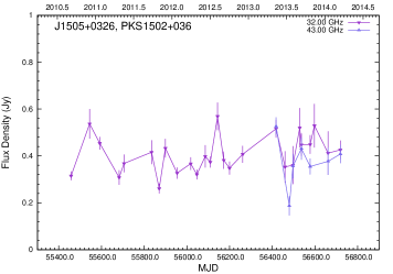
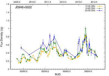
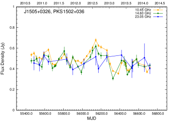
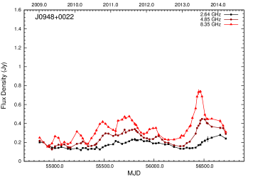
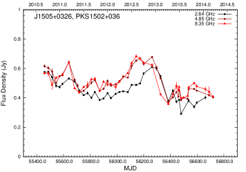
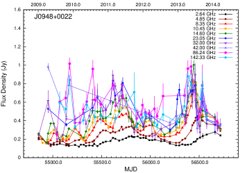
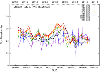
Figure 3: Radio light curves available for J0948$+$0022 (left column) and J1505$+$0326 (right column) at all available frequencies similar as is Fig. 2.

The dataset discussed here is the result of the longest-term multi-frequency radio monitoring for RL and $\gamma$-ray loud NLSy1s available. It covers the period between early-2009 and mid-2014. In Figs. 2 and 3 we present the available light curves at all observing frequencies. We only show measurements with a signal-to-noise ratio better than 3. All the light curves are also available online at the CDS. Table 7 is an example of an online light-curve file for J0324$+$3410 at 4.85 GHz. It contains the following information: Column 1 lists the MJD of a measurement, Col. 2 gives the flux density in units of Jy, and Col. 3 lists the associated error.

Table 7: Example of a light-curve file as published online at CDS. The current extract is for J0324$+$3410 at 4.85 GHz.

MJD	$S$	Error
	(Jy)	(Jy)
55408.300	0.485	0.006
55458.148	0.395	0.007
55487.059	0.440	0.011
55515.026	0.423	0.005
55570.904	0.374	0.005
…	…	…

The mean sampling – averaged over all frequencies – ranges from one measurement every 24 days for J0324$+$3410 and J0948$+$0022 (approximately the cadence of the most commonly used calibrator, 3C 286), and 29 days for J1505$+$0326, to more than 100 days for J0849$+$5108. Except for J0849$+$5108, for which the dataset does not cover a substantial number of activity cycles, the remaining three sources show intense variability at practically all frequencies, a behaviour commonly seen in blazars (e.g. Richards et al., 2011; Aller et al., 2011; Boettcher, 2012; Böttcher, 2004). The phenomenologies seen in these light curves vary significantly and mostly in terms of the observed amplitude of the different events. In these terms, J1505$+$0326 shows very weak outbursts. J0324$+$3410 shows at least two major events at the high-end of the bandpass at around MJD 56300 and 56600, which disappear at lower frequencies. J0948$+$0022 shows frequent recursive events of activity that occur considerably fast; their characteristic times are of the order of 40–50 days at the highest frequencies (see Table LABEL:tab:allflares). Most of the observed events can be identified at all frequencies (apart from the very low end of the bandpass) and with a time delay between frequencies (e.g. see event around MJD 56500 for J0948$+$0022), which is indicative of intense spectral evolution that is also routinely seen in blazar light curves (e.g. Rani et al., 2013). The variability amplitude is frequency dependent, following the typical fashion: higher frequencies vary more. For J0324$+$3410 for example, the amplitude of the most prominent event is more than twice as large at 32.00 GHz as at 14.60 and more than six times lesser at 10.45 GHz; yet another indication that the variability mechanisms seem to be the same as those acting in typical blazars (e.g. Valtaoja et al., 1992). Table 8 reports some characteristic parameters for these datasets. Specifically, for each frequency and source we report the total number of data points N, the dataset length $\Delta$t, the mean flux density $\left<S\right>$, the standard deviation around that mean $\sigma$, and the modulation index $m$.

In the following we roughly describe the most noteworthy phenomenological characteristics of the light curves separately for each source.

Table 8: Summary of the mean flux densities and corresponding standard deviations for each observing frequency and source presented in Figs. 2 and 3. For every entry we also report the number of data points N and the modulation index $m=100\cdot\sigma/\left<S\right>$ as a measure of the apparent variability amplitude. Only data points meeting the condition of S/N$\geq 3$ are included.

Source	Observable	Units		2.64	4.85	8.35	10.45	14.60	23.05	32.00	43.05	86.24	142.33
J0324$+$3410	N			42	45	48	48	43	14	27	8	17	17
	$\Delta$t	(days)		1310	1310	1310	1310	1310	1260	1260	517	899	899
	$\left<S\right>$	(Jy)		0.461	0.400	0.380	0.377	0.378	0.500	0.432	0.353	0.541	0.518
	$\sigma$	(Jy)		0.061	0.064	0.077	0.083	0.113	0.230	0.272	0.115	0.172	0.164
	$m$	(%)		13	16	20	22	30	46	63	32	32	32
J0849$+$5108	N			11	10	12	11	9	4	8	3	$\ldots$	$\ldots$
	$\Delta$t	(days)		981	581	1009	581	980	552	980	152	$\ldots$	$\ldots$
	$\left<S\right>$	(Jy)		0.203	0.214	0.244	0.266	0.287	0.363	0.391	0.529	$\ldots$	$\ldots$
	$\sigma$	(Jy)		0.012	0.019	0.028	0.028	0.040	0.043	0.103	0.079	$\ldots$	$\ldots$
	$m$	(%)		6	9	12	11	14	12	26	15	$\ldots$	$\ldots$
J0948$+$0022	N			56	63	63	65	57	31	43	14	30	23
	$\Delta$t	(days)		1863	1863	1863	1863	1862	1739	1862	1766	1644	1502
	$\left<S\right>$	(Jy)		0.177	0.255	0.356	0.390	0.442	0.555	0.488	0.569	0.596	0.530
	$\sigma$	(Jy)		0.039	0.086	0.142	0.157	0.173	0.155	0.188	0.226	0.193	0.169
	$m$	(%)		22	34	40	40	39	28	38	40	32	32
J1505$+$0326	N			37	42	39	43	37	15	26	7	$\ldots$	$\ldots$
	$\Delta$t	(days)		1204	1261	1261	1261	1261	1233	1261	301	$\ldots$	$\ldots$
	$\left<S\right>$	(Jy)		0.456	0.507	0.503	0.488	0.465	0.463	0.408	0.377	$\ldots$	$\ldots$
	$\sigma$	(Jy)		0.076	0.085	0.080	0.072	0.066	0.050	0.079	0.103	$\ldots$	$\ldots$
	$m$	(%)		17	17	16	15	14	11	19	27	$\ldots$	$\ldots$

4.1 J0324$+$3410

The multi-frequency light curves of J0324$+$3410 are shown in Fig. 2. It shows a clearly different behaviour between high- and low-frequency bands despite the rather sparse sampling. Of the main events present in the 86.24 and 142.33 GHz light curves – around MJD 56040, 56300 and 56620 – the first one disappears already at 10.45 GHz, the second is still present at 8.35 GHz, and the last can be traced down to 4.85 GHz. These events also show different characteristics such as rise and decay times. Generally, the source activity is very moderate at the lowest frequencies.

The neighbouring frequencies show associated events and strong evidence of intense spectral evolution. Differences between similar frequencies can be regarded as unusual because the events disappear fast over frequency. At the highest frequencies, flux density variations by factors of about 5 or more are present, which are absent at the lowest frequencies. The spectral evolution may be an even better proxy of this acute behaviour, as we discuss later.

Finally, we note that the baseline at all frequencies is practically flat, an indication that all the variability incidents evolve fast and dissipate in a dominating relic jet that either does not display any signs of variability or does so at a very slow pace; the dynamics of the radio SED shape point toward such an interpretation, as well.

4.2 J0849$+$5108

The very few available SEDs for this source indicate that this is another interesting and very active source. Unfortunately, the lack of a large enough and adequately sampled dataset prevents any systematic quantitative analysis. Nevertheless, the source shows activity cycles at all frequencies,which evolve systematically slower at lower frequencies (see the slow rising trend that becomes faster toward higher frequencies). It remains to be studied whether there is spectral evolution and what its characteristics are. Clearly, longer time-baselines are needed before any sensible results can be reached.

4.3 J0948$+$0022

J0948$+$0022 is among the best studied sources because it has been the first RL NLSy1 to be detected by Fermi. The light curves shown in Fig. 3 clearly indicate intense and repetitive variability that is prominent at all frequencies except possibly at 2.64 GHz, where most of the outbursting events have already smeared out. The light curves show variability corresponding to factors of more than 3 even at frequencies as low as 10.45 GHz or below. As an example, the light curve at 8.35 GHz undergoes a series of clearly discernible outbursts at MJDs, approximately 55020, 55240, 55490, 55725, 55985, and 56450. These events, which are single flares or sub-flares, appear in practically every densely enough sampled light curve except for that at 2.64 GHz (where the events have already disappeared). Even more interestingly, the moment of occurrence of an event appears at progressively later times as the frequency decreases, which indicates opacity effects. That is, a local maximum in a light curve corresponds to the instant at which the emitting plasma radiation becomes optically thin at the observing frequency. If the flare is associated with the emergence of an adiabatically expanding plasmon, this instant should indeed appear at progressively later times as the frequency drops. This claimed spectral evolution is very clearly seen in Fig.4 as we discuss below. Finally, the pace at which the observed flux density ($dS/dt$) increases during a flare is clearly a function of frequency, with higher frequencies showing much larger derivatives.

4.4 J1505$+$0326

The last source in our list of targets is J1505$+$0326. Its mean flux density of 507 mJy at 4.85 GHz, makes it the brightest member of the sample. Significant variability is also present, but with qualitatively different characteristics. The most important difference – at least compared with J0948$+$0022 – is that the clear spectral evolution with the delay of the peak as a function of frequency is not as obvious here. Pairs of adjacent frequencies such as 4.85 and 8.35 GHz seem to show events in phase, although the lowest frequency, 2.64 GHz, does indeed lag by clearly discernible time spans. At intermediate frequencies – for example at 10.45 GHz – the amplitude of variability reaches moderate factors of 1.5. Finally, frequencies below 10.45 GHz show a long-term decaying trend modulated by the faster variability discussed above.

5 Flare decomposition: parametrising variability

The parametrisation of flux density outbursts – in terms of amplitude and time scale – is commonly used as a method to constrain the variability brightness temperature $T_{\rm{var}}$ associated with the event, on the basis of causality arguments. The variability brightness temperature can only provide a lower limit of the intrinsic brightness temperature $T_{\rm{B}}$. Values of $T_{\rm{var}}$ in excess of independently calculated limiting values of the brightness temperature are generally attributed to Doppler boosting, which provides a handle for the computing limiting Doppler factors, $D$. Assuming an equipartition brightness temperature upper limit of $5\cdot 10^{10}$ K (Readhead, 1994), one can estimate the Doppler factors required to explain the observed excess.

The combination of variability Doppler factors with Very Long Baseline Interferometry (VLBI) measurements of the apparent speeds allows computing the plasmoid bulk velocity and jet viewing angle (e.g. Lähteenmäki & Valtaoja, 1999). Here, we are equally interested in all these properties for our four RL NLSy1s, and most importantly, in investigating the possible differences in the characteristics of different flares in the same light curve, rather than retrieving the characteristics of an average behaviour.

A practice commonly followed in variability studies is the implementation of time-series analysis methods that are designed to reveal such quantities; for example the structure function analysis (Simonetti et al., 1985) and the discrete correlation function (Edelson & Krolik, 1988). One of the most important caveats of such methods, however, is that they are extremely sensitive to parameters that are difficult to determine in moderately sampled light curves such as the onset of a flaring episode or the shape of the temporal behaviour of the measured flux density. In fact, even minor changes in such parameters can result in differences in the estimation of the variability brightness temperature beyond an order of magnitude. Furthermore, in most cases, these tools are designed to detect a dominant behaviour that smears out possible significant differences in the characteristics of individual flares of the same source and even at different observing frequencies.

To overcome such complications, we introduce a novel method for

1. first creating “cumulative” light curves by conveniently shifting and re-normalising the observed light curves. This operation is meant to highlight the flares that are detectable at a wide range of frequencies,

2. and subsequently subjecting those light curves to all necessary operations to extract the desired parameters (i.e. flare onset, duration, amplitude, etc.).

The guiding principles while developing this approach were to

1. avoid complications introduced by the superposition of simultaneously acting processes. For example, time-series analysis methods often return unrealistically long timescales only as the result of having – for example – a long-term almost-linear trend underlying much faster events.

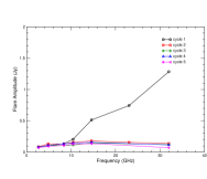
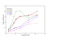
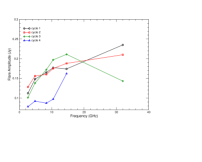
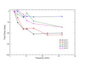
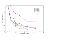
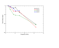
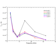
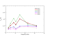
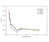
Figure 7: Left column: J0324$+$3410: top panel: the amplitude of the detected flares as a function of observing frequency with the cycle labels corresponding to the events seen in Fig. 2; middle panel: the flare delays; bottom panel: the $T_{\rm{var}}$ for the different activity cycles (flares) as a function of observing frequency. Middle column: J0948$+$0022. Right column: J1505$+$0326.

2. to accommodate a generic approach in the treatment of every flare. That is, to parametrise each event independently (for each source and frequency) and investigate the possibility of different behaviours (and possibly variability mechanisms) acting in the same source at different times. For J0324$+$3410, for example, the most prominent event seems to demand such an approach because its phenomenology is very different from the rest (Fig. 7)

All the details of the method are discussed in Appendix A.

5.1 Results of the flare decomposition

Since the variability brightness temperature $T_{\rm{var}}$ comprises only a lower limit of the brightness temperature $T_{\rm{B}}$, the higher the $T_{\rm{var}}$ estimate, the better $T_{\rm{B}}$ is constrained. Henceforth, from all the different estimates of $T_{\rm{var}}$ we compute in the following analysis, the highest value is regarded as the most meaningful one.

The method described above was applied to J0324$+$3410, J0948$+$0022, and J1505$+$0326, for which sufficiently long datasets were available and which showed a significant number of activity “cycles” (5, 6 and 4, respectively). Table 9 summarises the results of this analysis. The highest frequencies are missing clearly because of the lack of data points at these bands.

5.1.1 Flare decomposition for J0324$+$3410

Table LABEL:tab:allflares summarises the results of the flare decomposition method for all the significant events seen in the source light-curves shown in Fig. 2. As significant events are regarded flux variations that are above the noise level and can be detected at several wavelengths. As can be seen there, the variability of J0324$+$3410 is characterised by five fast variations shorter than 66 days (even at the lowest frequencies) with a relatively low amplitude; the largest amplitudes of the flares is generally reached at 14.60 GHz.

The flare occurring at around MJD 56313 shows exceptional characteristics. Its maximum is reached at 32.00 GHz, and at that frequency its amplitude is around ten times larger than the average of the other flares. The extraordinary phenomenology of this event alone could justify the introduction of an alternative analysis method like the one described here. A classical Structure Function analysis, for example, would have smeared the event out. Below 10.45 GHz it moderates its behaviour and displays amplitudes comparable to that of other events. Its temporal behaviour is similar to that of the immediately subsequent event which peaks around MJD 56356 at 32.00 GHz. The maximum time delay between 32.00 and 2.64 GHz is around 100 days for both flares, considerably longer than the estimated delays (between 20 and 70 days) for the other detected events. This might be an indication that the spectral evolution of the flares is temporarily modified by the onset of the main outburst.

The largest variability brightness temperatures are measured at 2.64 GHz. They all exceed $2\times 10^{12}$ K, implying a minimum Doppler boosting factor of $\sim 4.3$. In Fig. 7 we plot the time delays, the variability brightness temperature and the amplitude parameters for each flare separately.

5.1.2 Flare decomposition for J0948$+$0022

For J0948$+$0022, six prominent outbursts were identified in the light curves (Fig. 3, Table LABEL:tab:allflares), making the source a prototype for applying the discussed method. As can be seen in Fig. 7, for five of the six events the largest amplitude is seen at 32.00 GHz, while for flare 3 it is seen at 14.60 GHz. This is the result of high-frequency components that frequently appear at higher frequencies and expand fast towards lower bands. This behaviour is in accordance with the spectral evolution and the variability. The amplitude of the flares at different frequencies is shown in the upper panel of Fig. 7. Interestingly,

1. flares 1 and 2 are remarkably similar to each other, but very different from flares 4, 5 and 6. The latter three are relatively isolated events, while the former two occur at the peak of the outburst phase. It is likely that this is exactly the reason for the difference in the amplitudes.

2. flare 3 is different from all the others, with a large excess of flux at 14.60 and 10.45 GHz. The indications for an unusual spectral evolution of this event may be the interpretation of this phenomenology.

On the other hand the time delays, between different frequencies shown in the middle panel of Fig. 7 reveal a mildly different behaviour only for flare 5. Unfortunately, a gap in the 2.64 GHz data approximately where the peak is expected prevents us from excluding that the real time delays have to be shifted by about 30 days. Similarly, flare 3 at 2.64 GHz and flare 5 at 32.00 and 23.05 GHz cannot be well constrained because of inadequate sampling.

The largest $T_{\rm{var}}$ is measured at 14.6 GHz. In the lower panel of Fig. 7 we show $T_{\rm{var}}$ versus $\nu$ for the different flares. Most light curves give values of $T_{\rm{var}}$ roughly between 2 and $13\times 10^{12}$ K. The differences from flare to flare are small (drops in the flux density are partially compensated for by decreasing timescales), so that they cannot provide independent estimates of the variability brightness temperature. The flare models at different wavelengths, however, are independent of each other and hence the relatively small spread of $T_{\rm{var}}$ at different frequencies can be regarded as significant. The inferred values of $T_{\rm{var}}$ imply variability Doppler factors of the order of 5 to 7. The most prominent event occurred at around MJD 56444 (flare 3) and gave a $T_{\rm{var}}$ of more than $10^{13}$ K implying a $D$ of more than 8.7.

5.1.3 Flare decomposition for J1505$+$0326

Finally, for J1505$+$0326 we detected four main events during the monitored period as shown in Table LABEL:tab:allflares. They are all relatively fast and of moderate amplitude, more similar to the characteristics of J0324$+$3410 than to those of J0948$+$0022. The highest variability brightness temperatures reach values of $\sim 2\times 10^{13}$ K and are detected at 2.64 GHz, implying Doppler factors of almost 10.4. The spectral evolution of the flares seems to follow a standard pattern, with a long delay ($\approx$70 days) between 32.00 and 14.60 GHz and a considerably shorter one ($\approx$40 days) between 14.60 and 2.64 GHz.

Table 9: Variability parameters $T_{\mathrm{var}}$ and $D$ for the three sources whose datasets were long enough, and the frequency at which they are located. Here we report the highest values of $T_{\mathrm{var}}$.

Source	$\nu$	$T_{\mathrm{var}}$	$D$
	(GHz)	(K)
J0324$+$3410	2.64	$25\times 10^{11}$	4.3
J0948$+$0022	14.60	$13\times 10^{12}$	8.7
J1505$+$0326	2.64	$26\times 10^{12}$	10.4

6 Radio spectral energy distributions

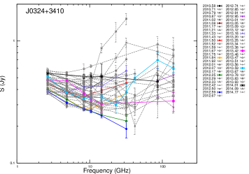
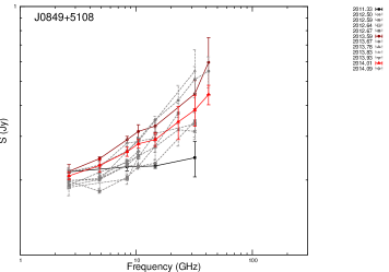
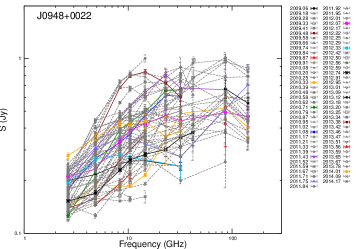
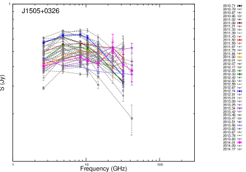
Figure 4: Radio SEDs of the four monitored NLSy1 galaxies. The data points are connected with straight segments to guide the eye. The legend denotes the fractional year for each SED.

Figure 4 shows the densely sampled broadband radio SEDs. There only data points with an S/N$\geq 3$ are shown. For guidance to the eye, the data points are connected with segments, and to avoid crowding the plots, only every fifth SED is coloured. In Table 10 a summary of their most characteristic parameters is given. These are the total number of available SEDs of at least two different frequencies, N; the average cadence quantified as the mean time-separation between two consecutive SEDs, $\frac{max(\mathrm{MJD})-min(\mathrm{MJD})}{N}$; the coherence,that is, the mean time-separation between the earliest and latest measurement in a SED, $max(\mathrm{MJD})-min(\mathrm{MJD})$; and the spectral index in three sub-bands computed from the mean flux densities in those bands. The spectral index is defined as $\alpha=d\ln S/d\ln\nu$, where $S$ is the measured flux density at a frequency $\nu$. As can be seen there, the mean cadence (excluding J0849$+$5108) is shorter than a month, and the combined Effelsberg-IRAM spectra are made of measurements synchronous within less than two days. It is reasonable to assume that the shapes of the individual SEDs are free of source variability effects.

From the plots in Fig.  4 it is evident that the mere sample of these four sources displays the main classes of spectral variability patterns described in Angelakis et al. (2012b). There, the variability patterns were interpreted as the result of the same underlying system consisting of a steep spectrum component attributed to a large-scale jet populated with high-frequency synchrotron components that evolve according to Marscher & Gear (1985). For Angelakis et al. (2012b) the different observed classes were governed by the amount of “activity” that the observing bandpass allows us to see, and was also caused by different intrinsic properties. Except for J1505$+$0326, where the spectral evolution is not discernible, all other three NLSy1 would be classified as type 1 or 2 in that classification scheme because they show an intense spectral evolution with or without a steep – presumably quiescent state – spectrum.

Table 10: Mean characteristics of the observed radio SEDs shown in Fig. 4. The spectral indices are computed in three sub-bands, and along with the mean values, the extremes are reported as well.

Source	N	Cadence	Coherence	low: 2.64 - 8.35 GHz				mid: 10.45 - 23 GHz				high: $\geq$43.05 GHz
		(days)	(days)	min	mean	max		min	mean	max		min	mean	max
J0324$+$3410	55	25	2.0	$-$0.49	$-$0.21	$+$0.12		$-$0.53	$-$0.04	$+$1.57		$-$0.67	$+$0.07	$+$0.77
J0849$+$5108	12	84	0.02	$+$0.04	$+$0.18	$+$0.44		$+$0.08	$+$0.32	$+$0.66		$+$0.28	$+$0.63	$+$1.08
J0948$+$0022	75	26	2.2	$-$0.13	$+$0.51	$+$1.26		$-$0.83	$+$0.27	$+$1.02		$-$1.73	$-$0.03	$+$1.58
J1505$+$0326	43	29	0.2	$-$0.22	$+$0.13	$+$0.34		$-$0.66	$-$0.18	$+$0.18		$-$0.86	$-$0.24	$+$0.07

6.1 J0324$+$3410

For J0324$+$3410 Fig. 4 clearly shows the emergence of two distinct components:

• A steep spectrum component that appears at frequencies below 10.45 GHz and mostly retains a constant negative spectral index that reaches values as low as almost $\approx-0.5$ (see Table 10) and could be the optically thin part of a synchrotron self-absorbed (SSA) component.

• A sequence of high-frequency components (HFC) that introduce intense variability as a result of their spectral evolution.

A convenient way to understand the reason for the observed behaviour is to examine the activity in terms of spectral index distribution in three different frequency sub-bands:

Low: for $\nu\in{[{\leavevmode\nobreak\ \leavevmode\nobreak\ 2.64}\leavevmode\nobreak\ ,\leavevmode\nobreak\ \leavevmode\nobreak\ \leavevmode\nobreak\ \leavevmode\nobreak\ 8.35]}$ GHz Middle: for $\nu\in{[{10.45}\leavevmode\nobreak\ ,\leavevmode\nobreak\ \leavevmode\nobreak\ 23.05]}$ GHz High: for $\nu\in{[{32.00}\leavevmode\nobreak\ ,142.33]}$ GHz.


In Fig. 5 we show the spectral index distributions in these sub-bands. The histograms are normalised so that they comprise the probability density functions (PDF) of the three indices. The bin size was selected to be similar (if not equal) to the mean standard deviation computed over the corresponding dataset. This representation compresses the behaviour and the phenomenology discussed earlier and immediately indicates the sub-band where the activity is mostly concentrated.

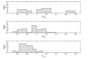
Figure 5: Probability density functions of the spectral indices observed for J0324$+$3410 in three different sub-bands: low, middle, and high. The bin size is selected to be approximately one standard deviation of the plotted indices.

As can be seen in Fig. 4, the region above roughly 10.45 GHz hosts all the source activity in terms of spectral evolution. It appears to be intensely variable, with the outbursting events emerging at the upper end of the band and transversing downwards following a characteristic evolutionary path; first a build-up at high frequencies, progressively harden as the flux increases, and a descent towards the left end of the bandpass while shifting the peak to lower flux densities to eventually diffuse in the persistent steep spectrum below 10.45 GHz.

This scheme agrees at least qualitatively with the evolutionary scenario proposed by Marscher & Gear (1985). The succession of these components and the superposition of their evolving spectra results in a flat average spectrum – with a spectral index practically around 0.0 – which at times can be as hard as $+1.6$ (see Table 10).

The steep spectrum component that dominates the SEDs at lower frequencies is not static. It shows variability in a self-similar fashion and mostly retains a steep character. The spectral index is positive for less than 7% of the time. The lowest indices ($\approx-0.5$, see also Fig. 5) indicate the canonical values seen in large-scale relaxed jets (e.g. Angelakis et al., 2009). A natural way to explain this behaviour is to assume that below about 10 GHz, the high-frequency components are optically thin. They transverse that part of the bandpass and slowly fade away and gradually contribute less and less power. This lets the overall spectrum appear to move downwards in flux density while preserving a rather constant index. This interpretation implies that high-frequency components with similar intrinsic parameters are generated (i.e. magnetic field and particle density). At the very low frequencies (2.64 and 4.85 GHz), the moderate spectral variability indicates an underlying large-scale jet. Essential in favour of this scenario would be the detection of significant polarisation in that part of the emission, as we discuss in Sect. 8.

The upper end sub-band ($\nu\geq 43.05$ GHz) can become as steep as of $\alpha\approx-0.7$ (Fig. 5), denoting that the transition from optically thick to thin regime of the HFC occurs in that spectral region. This occurs rather rarely; only 14% of the cases show such a steep index, most likely because as an event reveals its optically thin part, a new one emerges, that fast hardens the otherwise softening spectrum.

In the middle sub-band ($10.45\leq\nu\leq 23$ GHz), however the source spends half the time in soft and half in hard state since the “mixing” of thin and thick events is prominent there. In any case, the transition from thick to thin has very serious consequences because if proven true, it should be accompanied with exactly 90°rotations of the projected electric vector position angle (EVPA) as is described by Myserlis et al. (2014).

6.2 J0849$+$5108

The limited dataset available for J0849$+$5108 (see Fig. 4) already reveals a very interesting behaviour. First to be noted is the complete absence of any steep spectrum signature from the SEDs that have been gathered so far. The spectrum oscillates between flat and hard within all three sub-bands. As an example, the low sub-band spectral index varies between $+0.02$ and $+0.44$. In the high sub-band it reaches values higher than $+1$. Furthermore, the events always show their optically thick part, which – in the framework of incoherent synchrotron processes – is expected to be associated with an insignificant degree of linear polarisation. Clearly, more duty cycles are needed to allow better quantification of its spectral behaviour.

6.3 J0948$+$0022

The complete absence of a quiescence spectrum also holds for J0948$+$002. The spectra appear to be highly inverted and intensely variable. An impressive spectral evolution with HFCs emerging in the high sub-band is observed. The HFCs often transit to optically thin phases within the middle sub-band. Interestingly, the lowest band spectral index ($2.64\leq\nu\leq 8.35$ GHz) oscillates between a minimum of $-0.13$ and a maximum of $+1.26$, while the middle- and high-band indices oscillate between $-0.83$ and $+1.02$ and $-1.73$ and $+1.58$, respectively (c.f Fig. 6). This implies that we witnes the spectral evolution of the HFCs, but fail to detect the quiescent steep spectrum, if any. VLBI studies (e.g. Karamanavis et al. in prep.) also reveal only a compact core structure in agreement with the previous finding.

Furthermore, the relatively fast pace at which the spectral evolution occurs is interesting and rather exceptional. In fact, significant variability has previously been detected with a mean cadence of 25 days. This is also seen in the light curves, as discussed in Sect. 4.3. Figure 6 again gives the probability density functions of the three spectral indices as for J0324$+$3410.

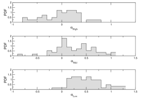
Figure 6: Probability density functions of the spectral indices observed for J0948$+$0022 in three different sub-bands: low, middle, and high. The bin size is selected to be approximately one standard deviation of the plotted indices.

6.4 J1505$+$0326

The behaviour of J1505$+$0326 is somewhat different from the behaviour of the sources discussed previously. Most of the time, it shows a convex spectrum that has a global maximum in the vicinity of 5 - 10 GHz and occasionally seems to be modulated by the evolution of HFCs that become optically thin. For that reason, it could be classified as type 5b in the scheme proposed by Angelakis et al. (2012c). The low sub-band spectral index reaches moderately hard states ($\max\left(\alpha\right)=+0.34$), while the high sub-band can become very soft ($\min\left(\alpha\right)=-0.86$).

7 Jet powers

Here we wish to quantify the power delivered by the four NLSy1s in our sample in the radio bands and examine whether this could be delivered by a jet similar to those in typical blazars.

Within the jet theoretical framework proposed by Blandford & Königl (1979) and empirical relations that have been proposed for relativistic jets in AGNs and galactic binaries by Foschini (2011a, 2012a, 2014), the radio measurements can accommodate the computation of the jet power (see also Foschini et al., 2014). In fact, it is possible to calculate both the radiative and kinetic (electron, proton, magnetic) jet power from the radio core emission. In a conical jet, the optically thick radio emission is linked to the jet power as

$$L_{\rm radio}\propto P_{\rm j}^{17/12},$$ (2)

By studying a sample of 88 $\gamma$-ray AGN (FSRQs, BL Lac Objects, RLNLS1s), Foschini (2014) found that the best normalisation coefficients values are

$$\log P_{\rm j,rad}=(12\pm 2)+(0.75\pm 0.04)\log L_{\rm radio,core}$$ (3)

$$\log P_{\rm j,kin}=(6\pm 2)+(0.90\pm 0.04)\log L_{\rm radio,core},$$ (4)

where $P_{\rm j,rad}$ and $P_{\rm j,kin}$ are the radiative and kinetic (proton, electron, and magnetic field) powers of the jet, while $L_{\rm radio,core}$ is the $K$-corrected luminosity of the radio core at 14.60 GHz. The $K$-correction was made by multiplying the monochromatic flux by the factor of $(1+z)^{\alpha-1}$, assuming a flat radio spectral index ($\alpha\approx 0$, see also Sect. 6).

Although it would be possible to use different frequencies as well, we persist in using 14.60 GHz for a number of reasons, such as to be consistent with the measurements used to extract the used normalisation coefficients; the good sampling of the corresponding light curve; the fact that this band is less contaminated by extended emission, which gives more reliable estimates of the radio core emission; it allows comparison with other projects such as MOJAVE (Kellermann et al., 2004; Lister et al., 2009, 2013).

In Table 11 we provide the naturally weighted averages of the radiative $P_{\rm{j,rad}}$, kinetic $P_{\rm{j,kin}}$, and total powers $P_{\rm{j,tot}}$. The averaging was made in the power rather than the flux density domain. In the same table we present the most recent estimates for the black-hole masses (Foschini et al., 2014).

Table 11: Radiative and kinetic jet powers calculated from the 14.60 GHz observations averaged over the period discussed here. Literature values of their black-hole masses are as well.

Source	$P_{\rm{j,rad}}$	$P_{\rm{j,kin}}$	$P_{\rm{j,tot}}$	$\log\rm{M}^{1}$
	(erg s-1)	(erg s-1)	(erg s-1)	($\log\rm{M}_{\sun}$)
J0324$+$3410	$1.7\times 10^{43}$	$3.0\times 10^{43}$	$4.7\times 10^{43}$	7.6
J0849$+$5108	$6.6\times 10^{44}$	$2.5\times 10^{45}$	$3.1\times 10^{45}$	7.5
J0948$+$0022	$7.9\times 10^{44}$	$3.0\times 10^{45}$	$3.7\times 10^{45}$	7.9
J1505$+$0326	$5.0\times 10^{44}$	$1.7\times 10^{45}$	$2.2\times 10^{45}$	7.3

(1) Foschini et al. (2014)

7.1 J0324$+$3410

The prominent event seen in the source light-curves at around MJD 56300 (January 2013) gave a corresponding increase in the radio power at that time. Tibolla et al. (2013) reported a change in the X-ray spectrum from January to February 2013 associated with that event, with the emergence of a hard tail during the second epoch. The average values of the radiative $P_{\rm{j,rad}}$ and kinetic jet power $P_{\rm{j,kin}}$ – as measured in the present work – are $1.7\times 10^{43}$ and $3.0\times 10^{43}$ erg s^-1. The same quantities calculated from the SED modelling by Abdo et al. (2009c) after the first year of the satellite operations were $6.3\times 10^{42}$ and $2.2\times 10^{44}$ erg s^-1.

7.2 J0849$+$5108

Unfortunately, the limited dataset available for J0849$+$5108 is not adequate to reveal the source activity characteristics. Furthermore, available measurements are not simultaneous to the $\gamma$-ray active phase it went through in 2010 (Foschini, 2011b). The radiative jet power reported by D’Ammando et al. (2012, 2013c) is around $(5-50)\times 10^{44}$ erg s^-1 (the maximum refers to the outbursts), which is consistent with our calculations, which gave an average of $6.6\times 10^{44}$ erg s^-1.

7.3 J0948$+$0022

J0948$+$0022 was extensively studied by Foschini et al. (2012), who discussed the results of more than three years of multi-wavelength data over the period between 2008 and 2011. They presented the calculations of jet powers in terms of SED modelling. With the current work – which comprises the natural extension of that monitoring to mid-2014 – we can compare these findings with those of the currently applied method for the overlapping period. A caveat of the SED modelling has been the delay of the radio emission with respect to the optical-to-$\gamma$-ray emission, as is generally expected. Fuhrmann et al. (2014) found that the average time delays at the source rest frame can span from less than 10 to more than 70 days, systematically decreasing towards higher frequencies, which provides yet another argument in support of using the 14.60 GHz for the current calculations.

The radiative powers computed by Foschini et al. (2012) were based on SEDs that were selected on the basis of the $\gamma$-ray activity. During the lowest activity SED, the jet radiative power was estimated to be $P_{\rm{j,rad}}=0.4\times 10^{45}\mathrm{\leavevmode\nobreak\ erg\leavevmode\nobreak\ s}^{-1}$, while during the highest activity state it was $P_{\rm j,rad}=7.9\times 10^{45}\mathrm{\leavevmode\nobreak\ erg\leavevmode\nobreak\ s}^{-1}$. From our radio dataset, the radiative power ranges between $0.4$ and $1.8\times 10^{45}\mathrm{\leavevmode\nobreak\ erg\leavevmode\nobreak\ s}^{-1}$. For the jet kinetic power, the SED modelling applied by Ghisellini & Tavecchio (2009) showed that it ranges from $0.2$ to $4.1\times 10^{47}$ erg s^-1, while based on the 14.60 GHz measurements of the present work, it varies in the range between $1.5$ to $7.8\times 10^{45}$ erg s^-1. This result is very interesting when the fundamental assumptions are considered. The kinetic jet power – as calculated from the SED modelling – relies on the assumption that there is one proton associated with each electron (Sikora & Madejski, 2000). If that were not the case and instead there were one proton for more electrons, the kinetic power would be much lower, which is what our finding indicates.

7.4 J1505$+$0326

The multi-frequency light curves of J1505$+$0326 show at least one major event with mild spectral evolution. Despite its mild variability, we can compare, our values with those from SED modelling reported in Abdo et al. (2009c). $1.0\times 10^{44}$ and $1.6\times 10^{46}$ erg s^-1 are the values of the radiative and kinetic jet powers. The averages we calculated are $5.0\times 10^{44}$ and $1.7\times 10^{45}$ erg s^-1, respectively. The almost constant activity of the source is consistent with what was reported by D’Ammando et al. (2013a), who analysed the monitoring at 15 GHz performed by the Owens Valley Radio Observatory (OVRO).

8 Polarisation

Assuming that the dominant radiation mechanism is incoherent synchrotron processes and that the variability is attributed to evolving synchrotron self-absorbed components, it is expected that significant linear polarisation is detected. In this context, the degree of polarisation and the EVPA would depend on the emitting plasma opacity and hence the spectral index (Pacholczyk, 1970, 1980). Assuming highly ordered and intense magnetic fields (Sciama & Rees, 1967), as those expected during flares, even circular polarisation could occur. Furthermore, the orientation of the electric vector should also depend both on the optical thickness of the material and on the assumed magnetic field configuration. Multi-band polarisation studies are then a unique probe of the underlying physical conditions at the emission region.

For the sample discussed here, Neumann et al. (1994) found optical polarisation from J0324$+$3410, while Moore & Stockman (1981) and Sitko et al. (1984) detected “high and variable optical polarisation” from J0849$+$5108. This has been seen as an indication that a relativistic jet is operating at the source. Similarly, Doi et al. (2012) have detected significant polarisation in the radio.

8.1 Radio polarisation

Angelakis et al. (2013) explored the possibility of detecting radio linear polarisation at the intermediate frequency of 8.35 GHz. The data in Table 3 there were corrected for instrumental polarisation and indicated that all four sources display detectable polarisation of a remarkably low magnitude. Exceptionally, J0324$+$3410 showed values higher than those typically observed in AGN at these frequency bands ($\sim 4$ % at 5 GHz, e.g. Klein et al. 2003). Its fractional linear polarisation at this frequency is about 6 % with an EVPA of about 36°, while at 4.85 GHz it reaches values of 7 % with an EVPA of about 44°. This phenomenology would agree with assuming that the optically thin emission dominates towards lower frequencies. The 4.85 GHz emission is less contaminated by the optically thick part of an HFC and displays a higher fractional polarisation. At both frequencies the EVPA appears to be almost perpendicular to the jet orientation (the jet axis is about 120°, Karamanavis et al. in prep.), so that the projected magnetic field appears to lie almost parallel to the jet, possibly implying a helical jet with a very long helix step.

Similar arguments hold for J0849$+$5108, although the effect is much more moderate. Unlike J0324$+$3410, the other NLSy1s show a very low polarisation degree. As is indicated by their spectral variability pattern, the sources undergo flaring events that show their optically thick part at 8.35 GHz.

8.2 $R$-band polarisation

First attempts to monitor the $R$-band linear polarisation in 2013 with the RoboPol instrument (King et al., 2014; Pavlidou et al., 2014) showed that J0324$+$3410 and J0948$+$0022 present a rather low fractional polarisation that does not exceed a few percent ($\approx 3$ %). Itoh et al. (2014) found similar values for the former case, while the latter showed past events of polarisation values that reached almost 40 % (Itoh et al., 2013). For J0849$+$5108 we detected polarisation levels of about 10 %.

9 Discussion

The main goal for the analysis has been to study the relativistic jets that emit the observed radio power and to quantify its properties. The discussed dataset comprises the longest term multi-wavelength radio monitoring datasets of the known $\gamma$-ray-detected NLSy1s to date.

The focus was placed mostly on the variability properties of the radio emission. In this context, we follow different paths. We introduced a flare decomposition algorithm to quantify the variability amplitude, the involved timescales, and its frequency dependence for each flare separately. We then examined whether variability retains the same characteristics over source, frequency or event. Subsequently, the variability parameters (amplitude and time scale) served as the base for computing the limiting values for the variability brightness temperatures and the corresponding Doppler factors. In the frequency domain, much attention was given to the spectral evolution seen in each source, chiefly because of the signatures that the variability mechanisms leave in the evolutionary path followed by the flaring events. Furthermore, the power delivered by source in the radio regime was computed at one selected frequency and was compared with the powers seen in the jets of typical blazars. Finally, the radio and the optical polarisation was investigated as a signature of relativistic jet emission.

The mean flux densities are between 200 and 600 mJy. All sources appear significantly variable at cm and mm bands, except maybe J0849$+$5108, for which it is rather premature for such a statement to be made. The flare decomposition algorithm revealed several events in each light curve. The characteristics of different events can vary even in the same light curve, implying that either the underlying mechanism is not the same, or that each time different evolutionary stages are detected. The delays between the peaks at different frequencies of the same event range between a few days, tenths of days, and 180 days, showing a power-law frequency dependence. The flare timescales range between $\approx 30$ and 200–300 days. The computed highest variability brightness temperature $T_{\rm{var}}$ is between $10^{12}$ and $10^{13}$ K. Consequently, values ranging from 4.3 to 10.4 were found for the corresponding Doppler factor, $D$.

From examining the behaviour in the frequency domain, it is immediately clear that intense variability occurs in the same ways as routinely seen in blazars. Specifically, the variability events seem to appear at high frequencies and evolve downwards in frequencies, following an evolutionary path seen in blazar flares. Interestingly, the power of the events is a significant part of the overall power. Apart form the case of J0324$+$3410 that shows signs of a steep underlying spectrum the rest give no hints for such in our bandpass.

The 14.60 GHz radio power ranges roughly between $10^{43}$ and $10^{45}$ erg s^-1 in agreement with what should be expected from a relativistic jet. The 8.36 GHz polarisation data indicated low degree of fractional polarisation for three of our sources. For J0324$+$3410 however it reached values up to almost 6 %. Strong indication that we are dealing with the non-thermal emission originating at a relativistic jet which is even dominating over a core emission despite the source compactness at VLBI scales. Despite the interesting findings of first attempts to conduct optical linear and radio linear and circular polarisation study (that we have already discussed in Sect. 8 and will discuss below), a methodical and complete polarisation analysis will be presented in subsequent publication after longer optical polarisation time baselines are completed.

9.1 J0324$+$3410

As we extensively discussed in Sect. 4, the source light-curve has similar characteristics as blazars with the only exception of the moderate average flux densities. In combination with the picture drawn from the radio – almost monthly sampled – SEDs and their measured spectral indices, this points to the scenario of a jet within which high-frequency components are generated. The HFCs subsequently evolve transversing the possible opacity phases, before disappearing with an expansion towards low frequencies (Marscher & Gear, 1985; Türler et al., 2000). The emergence of later events of similar phenomenology indicates that the physical conditions are stable (particle densities, magnetic field strength) at the location of the emission and could be in accordance with a reoccurring activity that would result from a stable or, a slowly evolving acceleration region. The variability of J0324$+$3410 is characterised by fast variations – shorter than 65 days, even at the lowest frequencies – with relatively low amplitude. From the flare decomposition exercise we estimate that the highest brightness temperature limits are all higher than $2\times 10^{12}$ K, implying a Doppler boosting factor of at least 4.3, rather low compared with the variability values seen in blazars (e.g. Hovatta et al., 2009).

An essential element of the exact processes operating at the source would be studying of polarisation behaviour at radio and optical wavelengths. As was discussed earlier, J0324$+$3410 displayed fractional linear polarisation of about 6 % and 7 % at 8.35 GHz and 4.85 GHz, respectively (Angelakis et al., 2012a). This increase towards lower frequencies might be an indication that optically thin emission – arguably from a relativistic jet – becomes progressively dominant towards lower frequencies. At higher frequencies the emission is dominated by optically thick (and hence less polarised) emission of an evolving HFC. In the optical regime the detected significant polarisation has been seen as evidence of an, at least mildly, relativistic jet (Yuan et al., 2008). Our $R$-band RoboPol monitoring (King et al., 2014; Pavlidou et al., 2014) showed that the optical polarisation of the source is very low and shows fluctuations between 1 and 3 %. Its $R$-band magnitude is almost stable at roughly 15.3 mag. A possible explanation for this unusually low value of the optical polarisation may be the contamination of the emission with an unpolarised stellar component that would result a lower net polarisation.

Finally, the total jet powers computed from our 14.6 GHz dataset agree well with those computed with SED modelling that accounts for all different emission components. In conclusion, there is compelling evidence that the source radio emission is dominated by a jet emission that shows characteristics often seen in blazars, but not necessarily as powerful.

9.2 J0849$+$5108

Unfortunately, the limited number of observations that have been performed on the source do not allow a proper light curve analysis. The radio SED, however, already reveals clear signs of – at least mild – spectral evolution indicative of recursive activity, a typical characteristic of radio blazars. Its spectral index shows variability at all sub-bands (see Sect. 6) and reaches values of $+1$, indicating that our bandpass samples a part of the spectrum where most of the radio activity occurs. The dominance of the assumed optically thick emission could also explain the very low radio polarisation.

9.3 J0948$+$0022

The detection of J0948$+$0022 as a $\gamma$-ray emitter (Abdo et al., 2009a) triggered the monitoring programme we discussed here. Consequently, its light curves are the best sampled. It is very radio-loud (Zhou et al., 2003), in contrast to the typical NLSy1s, and displays light curves with clear intense variability. Its radio SED shown in Fig. 4 reveals a very interesting case with sequential HFC appearing at high frequencies, evolving through the bandpass before fading with the emergence of a new component. The lowest band spectral index shows values as inverted as $+1.26$, while the high band spectral index can be as steep as $-1.73$, implying that the source activity occurs within our bandpass. A careful cross-correlation of spectral index trains with the associated radio polarisation will be key to really proving the presence of the HFC that cause the variability; this would favour a typical blazar-like jet.

From the flare decomposition it appears that the best constraint in the variability brightness temperature is set by the 14.60 GHz measurements and gives values $13\times 10^{12}$, implying a variability Doppler factor of $\sim 8.7$. Karamanavis et al. (priv. comm.) have been trying to detect moving components in 15 GHz MOJAVE data for the purpose of measuring apparent speeds. However, the source appears to be unresolved. In conclusion, it could be said that this source resembles most the typical blazar behaviour of the four sources in our sample.

In Sect. 7.3 we discussed that the jet powers computed from SED modelling (Foschini et al., 2012) are more than an order of magnitude larger that those computed here. Interestingly, this could be an indication that the jet composition is different from the composition assumed for SED modelling.

Recently, D’Ammando et al. (2014) reported the detection by Fermi of a strong $\gamma$-ray flare observed between December 2012 and January 2013 in the 0.1–100 GeV energy range. Its peak occurred at MJD 56293. A quasi-simultaneous flare was observed from optical to X-rays, suggesting a tight connection of the corresponding emitting regions. The examination of OVRO 15 GHz light curves showed no flaring activity at the time of the $\gamma$-ray flare. A strong radio peak was instead observed in June 2013. The authors hypothesised that there might be a delay between the $\gamma$-ray and the radio activity of about five months, due to opacity effects and propagation of the shock along the jet. The case becomes very interesting when examining our light curves, which show the detection of a radio-flare quasi-simultaneous to the $\gamma$-ray flare. As can be seen in Fig. 4, the 23.05 GHz data show a very prominent flare. It starts at the beginning of December 2012, peaks between December 15 and January 4, 2013, and ends at the beginning of February 2013. The flare is weaker in the 32.00 GHz light curve, while at 14.60 GHz it is practically invisible. Unfortunately, the insufficient sampling of highest frequencies in our programme prevent us from quantifying the flare dependence in frequency. Our data suggest that the $\gamma-$ray flare propagates to radio frequencies down to $\sim$23.05 GHz with almost no time delay, showing that the propagation of the shock along the jet is fast. At lower frequencies, the flare drops drastically, probably because of opacity effects. The examination of the radio SED implies a subtle HFC that barely reaches the centre of our bandpass before it disappears. In any case, the sudden disappearance of the event as a function of frequency demands more investigations of the mechanisms behind the very broadband emission (from $\gamma$ rays to radio) and its evolution.

9.4 J1505$+$0326

The radio SED of J1505$+$0326 differs from the usual behaviour seen in the other NLSy1s in our sample. Its spectrum is most often convex with its peak in the range of 5–10 GHz. Occasionally, there appear signs of evolution caused by an HFC entering the bandpass. It is essential, however, that the total number of available cycles does not allow deciding whether the spectrum is intrinsically convex or whether it possibly changes at a slow pace.

The flare decomposition detected four rather short events and have moderate amplitude despite the source’s radio-loudness. The highest variability brightness temperature limit was computed at 2.64 GHz and yielded values of $\sim 2.6\times 10^{13}$ K, implying a boosted relativistic jet with Doppler factors of more than 10.

10 Conclusions

Before we conclude, we emphasise that our findings cannot necessarily be assumed to be representative of all RL, $\gamma$-ray NLSy1 galaxies. The most outstanding findings of this work are as follows:

1. We presented the most systematic radio monitoring of RL and $\gamma$-ray-detected NLSy1s to date. The obtained light curves spread over periods longer than five years. The acquired dataset includes eight frequency bands between 2.64 and 142.33 GHZ and is available online for the community for further studies.

2. The light curves show the typical phenomenology seen in blazars, although they generally have lower flux densities. All of them show variability events that in most cases have a smaller amplitude, however. Sometimes very prominent and energetic events appear and dominate the light-curve appearance.

3. We introduced an alternative method for detecting flares and quantifying their characteristics, which – contrary to the traditional methods – is approaching the problem on the basis of individual flares. In that context, the properties of each flare can change over frequency; similarly, the different events in the same light curve can appear with different properties, which indicates either different variability mechanisms or a different flare evolution stage.

4. The flare decomposition method showed that the computed variability brightness temperatures are in general moderate – in contrast to the majority of blazars –, implying Doppler factors that do not exceed about 10. The operating jet then must be moderately relativistic.

5. The same method showed that the duration of the events is somewhat shorter than what is seen in blazars, resulting in slightly more frequent events.

6. For the three cases where longer periods have been covered, the radio SEDs clearly show intense variability that is mostly characterised by clear spectral evolution of the events. The evolution seems to occur slightly faster than in blazars – as was also indicated by the results of the flare decomposition – but follows patterns possibly caused by evolving internal shocks. Furthermore, in one case the shape of the radio SED towards the lower frequencies gives a direct indication of a quiescent jet (steep spectrum, steady).

7. The jet power estimations gave values in accordance with jet outputs comparable to the least energetic blazars (BL Lac objects). For J0948$+$0022 the comparison with SED modelling results indicates lower values that may be attributed to different p-e ratios in the jet.

8. The first multi-frequency radio polarisation results showed that our sources have shown very low or negligible polarisation. In contrast, J0324$+$3410 a displayed polarisation degree of 6 and 7 % at 8.35 and 4.85 GHz. This is rather high, especially given the compactness of the source, and could be explained by the jet dominating the core in the total power. The increase towards lower bands is in accordance with that assumption as more and more optically thin emission from an underlying jet becomes detectable. From the above it becomes rather evident that

9. a mildly relativistic boosted jet must be operating at these sources and probably is responsible for the observed radio emission. This jet lie, probably towards the low end of the energy distribution, however.

10. The characteristics of its radio emission are qualitatively similar to those in blazars, but are generally less intense. The spectral evolution seems to occur at a faster pace, involving shorter timescales probably related to the systematically smaller black-hole masses or higher accretion rates.

11. In the particular case of J0948$+$0022, a flare detected by Fermi towards the end of 2012 seems to be present in our 23.05 GHz dataset, but is practically absent at frequencies below that. This unusual behaviour deserves further investigation of the possible mechanism that could cause such an abrupt flare disappearance.

Appendix A flare decomposition method

The detection and parametrisation of different flares (which are then used to compute the associated variability brightness temperature) requires solving several problems, most of which have to do with the paradox that before an independent parameterisation of all flares is reached, we need to identify their average shape and spectral evolution, minimise the arbitrariness of the results. The problems to be addressed can be summarised as follows:

1. We ned to identify of the strongest flare, accounting for the fact that its amplitude may strongly depend on frequency so that the strongest flare at one frequency may be a minor event at others.

2. We also need to localise of the same flare at different frequencies, given its spectral evolution.

3. The flares need to be modelled efficiently using the minimum number of free parameters.

4. Finally, we have to test and possibly correct the model to optimise the results.

The implementation of these steps was made as follows:

1. We estimated the average time delays between the flux density variations detected in different light curves. The main complication in this procedure is the fact that using a standard cross-correlation function (see Edelson & Krolik, 1988; Lehar et al., 1992) on pairs of light curves does not ensure consistent results. For example, assuming the estimated delays between three light curves $a$, $b$, and $c$ to be $\tau_{a,b}$, $\tau_{a,c}$ and $\tau_{b,c}$, it might well be that $\tau_{a,c}\neq\tau_{a,b}+\tau_{b,c}$. A solution of this problem is to include all the possible pairs of light curves when calculating the time delays. By visual inspection, a maximum time delay between light curves, $\tau_{max}$, is identified. Then, for every pair of light curves $i$ and $j$ with $i<j$, a cross-correlation function $r_{i,j}(\tau_{i,j})$ is calculated for any time delay $\tau_{i,j}$ in the range ($-\tau_{max},\tau_{max}$). For $n$ monitored frequencies an overall correlation function can be calculated as

   $$R(\tau_{1,2},\tau_{2,3},...,\tau_{n-1,n})=\prod_{i,j}r_{i,j}(\tau_{i,j}),$$ (5)

   where

   $$\begin{array}[]{lp{0.8\linewidth}}\tau_{i,j}=\tau_{i,i+1}+\tau_{i+1,i+2}+...+\tau_{j-1,j},&\\ \end{array}$$

   We computed $R$ for any possible set of time delays, excluding all the combinations involving $r_{i,j}(\tau_{i,j})<0$. The most significant set of time delays was selected as the one providing the highest overall correlation value.

2. We composed a “cumulative” light curve, in which the strongest flare was identified. The light curves were shifted in time by the best fit delays found in the previous step, so that their variations were aligned. Their fluxes were normalised by their standard deviation, to have similar variations at all wavelengths. Assuming for example that all the variations at 86.24 GHz have an amplitude of 1 Jy and at 2.64 GHz have an amplitude of 0. Jy, they all count the same for the identification of the flares. This way, we ensured that our detection algorithm was not biased towards the highest frequencies. The resulting light curves were merged to create one well-sampled total “cumulative” light curve. The merging of the light curves does not require averaging; the points from all the light curves are combined regardless of the frequency at which they were observed. The previous steps are meant to make all points equivalent, giving us the opportunity create a well-sampled light curve in which every data point from every frequency participates with the same weight. To construct the cumulative light curve, one could identify the following steps:

3. We identified the strongest flare. The cumulative light curve was smoothed (with an adaptive smoothing factor) and localised the highest flux density.

4. We localised the same flare at different frequencies. Knowing the average time delays between variations occurring at different frequencies, the strongest flare can be identified in each of the actual light curves. Gaussian fit models, different for each wavelength, were applied to the actual light curves to determine the amplitude and timescale of the strongest flare; they were then subtracted from the original flux densities, creating a new set of light curves (one per wavelength) for which all the steps from step 3 on are repeated. The procedure was iterated until no other significant flares are detected.

5. Model test. The residual light curves were checked to verify that no peaks or dips are systematically present in the position of the subtracted flares. Their existence would indicate that the flares are not properly modelled; new models would be created and the whole procedure repeated until a satisfactory result is reached.

This approach has the advantage of individually localising and modelling each event. Once a flare is detected in a cumulative light curve, the average time delays returned by step 1 allow us to infer its approximate position in the real light curves. The accurate position is then identified from the flux peak closest to the approximate position. In this way, we are able to estimate the actual time delays as a function of wavelength for each flare separately, and therefore detect possible variations in their spectral evolution. Naturally, the procedure also provides information about how the amplitude and the rising and decaying times of the flares vary with wavelength, which leads to a full parametrisation of the flux density variations observed in the sources; this is necessary to compute brightness temperatures.

Appendix B Results of the flare decomposition

Here we append the results of the flare decomposition method described in Sect. 5.1.

Table 12: Results of the flare decomposition for all three sources.

$\nu$	Time	Amplitude	Peak	Time	$T_{\mathrm{var}}$	$D$
	delay		position	scale
(GHz)	(d)	(Jy)	(MJD)	(d)	($10^{11}$ K)
J0324$+$3410
Flare 1
32.00	$-$100	1.284	56313	46	4.6	2.2
23.05	$-$101	0.744	56312	38	8.0	2.7
14.60	$-$105	0.514	56308	33	18	3.6
10.45	$-$82	0.205	56331	47	6.9	2.6
8.35	$-$81	0.133	56333	65	3.9	2.2
4.85	$-$52	0.105	56362	64	8.6	2.9
2.64	0	0.081	56413	61	25	4.3
Flare 2
32.00	$-$108	0.139	56356	32	1.0	1.3
23.05	$-$109	0.157	56355	30	2.7	1.9
14.60	$-$78	0.180	56385	29	8.1	2.7
10.45	$-$79	0.157	56384	45	5.8	2.4
8.35	$-$82	0.130	56381	65	3.8	2.2
4.85	$-$30	0.132	56433	66	10.2	3.1
2.64	0	0.086	56463	63	24	4.3
Flare 3
32.00	$-$73	0.121	55747	30	1.0	1.3
14.60	$-$45	0.146	55775	29	6.5	2.5
10.45	$-$8	0.114	55812	45	4.2	2.2
8.35	$-$29	0.108	55791	64	3.1	2.0
4.85	$-$14	0.108	55806	64	8.9	3.0
2.64	0	0.084	55820	63	24	4.2
Flare 4
32.00	$-$24	0.116	55638	30	1.0	1.3
14.60	$-$26	0.158	55636	29	7.1	2.6
10.45	$-$23	0.145	55639	45	5.4	2.4
8.35	$-$25	0.133	55638	65	3.9	2.2
4.85	$-$2	0.110	55661	64	9.0	3.0
2.64	0	0.081	55662	61	25	4.3
Flare 5
32.00	$-$73	0.072	56183	26	0.8	1.2
14.60	$-$57	0.137	56199	27	7.0	2.6
10.45	$-$43	0.128	56213	45	4.7	2.3
8.35	$-$15	0.108	56240	65	3.1	2.0
4.85	5	0.093	56260	64	7.7	2.8
2.64	0	0.070	56256	61	21	4.1
J0948$+$0022
Flare 1
32.00	$-$175	0.400	55617	44	53	7.6
23.05	$-$179	0.320	55614	50	69	7.1
14.60	$-$153	0.305	55640	61	102	8.1
10.45	$-$148	0.249	55644	103	57	6.7
8.35	$-$92	0.198	55700	103	76	6.6
4.85	$-$87	0.098	55705	146	51	5.9
2.64	0	0.064	55792	268	34	5.3
Flare 2
32.00	$-$168	0.337	55705	42	49	7.4
23.05	$-$159	0.332	55715	50	71	7.2
14.60	$-$153	0.309	55721	61	103	8.1
10.45	$-$128	0.267	55745	103	61	6.9
8.35	$-$92	0.185	55782	101	73	6.6
4.85	$-$65	0.101	55808	146	53	6.0
2.64	0	0.058	55874	260	32	5.2
Flare 3
32.00	$-$171	0.331	56406	42	48	7.4
23.05	$-$168	0.277	56409	50	60	6.8
14.60	$-$133	0.408	56444	62	133	8.7
10.45	$-$133	0.400	56444	110	81	7.5
8.35	$-$125	0.306	56452	108	106	7.3
4.85	$-$96	0.138	56481	151	68	6.4
Flare 4
32.00	$-$173	0.320	55446	42	46	7.3
23.05	$-$161	0.240	55458	50	52	6.5
14.60	$-$146	0.119	55473	55	48	6.4
10.45	$-$139	0.105	55479	93	30	5.5
8.35	$-$131	0.094	55487	94	43	5.6
4.85	$-$96	0.062	55523	137	37	5.4
2.64	0	0.037	55619	230	26	4.9
Flare 5
14.60	$-$71	0.092	54998	52	42	6.1
10.45	$-$56	0.071	55013	91	21	5.0
8.35	$-$41	0.053	55028	87	29	5.0
4.85	7	0.038	55076	128	26	4.9
2.64	0	0.026	55069	206	23	4.7
Flare 6
32.00	$-$168	0.180	55978	37	33	6.5
23.05	$-$170	0.163	55976	45	43	6.2
14.60	$-$175	0.095	55972	52	43	6.2
10.45	$-$157	0.098	55989	93	28	5.4
8.35	$-$147	0.084	55999	92	40	5.5
4.85	$-$105	0.059	56041	137	35	5.3
2.64	0	0.032	56146	221	24	4.8
1505$+$0326
Flare 1
32.00	$-$104	0.235	55545	29	48	7.4
14.60	$-$37	0.174	55611	50	58	7.6
10.45	$-$10	0.177	55639	80	44	6.9
8.35	$-$13	0.165	55636	78	72	6.9
4.85	$-$5	0.148	55643	99	111	7.9
2.64	0	0.112	55649	109	233	10.0
Flare 2
32.00	$-$120	0.210	56146	26	52	7.6
14.60	$-$33	0.188	56233	50	62	7.8
10.45	$-$32	0.175	56234	80	44	6.9
8.35	$-$30	0.160	56235	78	70	6.8
4.85	$-$8	0.156	56257	103	108	7.8
2.64	0	0.128	56266	111	258	10.4
Flare 3
32.00	$-$107	0.143	56088	25	39	6.8
14.60	$-$55	0.211	56140	50	70	8.1
10.45	$-$53	0.197	56141	84	45	6.9
8.35	$-$49	0.172	56145	78	75	7.0
4.85	$-$21	0.138	56173	99	103	7.7
2.64	0	0.101	56194	107	219	9.8
Flare 4
14.60	$-$27	0.162	55809	48	58	7.6
10.45	$-$29	0.097	55808	77	27	5.8
8.35	$-$16	0.087	55821	73	44	5.9
4.85	$-$5	0.092	55831	95	75	7.0
2.64	0	0.078	55836	103	181	9.2

Table 12: continued.