A Particle Multi-Target Tracker for Superpositional Measurements using Labeled Random Finite Sets

Abstract

In this paper we present a general solution for multi-target tracking with superpositional measurements. Measurements that are functions of the sum of the contributions of the targets present in the surveillance area are called superpositional measurements. We base our modelling on Labeled Random Finite Set (RFS) in order to jointly estimate the number of targets and their trajectories. This modelling leads to a labeled version of Mahler’s multi-target Bayes filter. However, a straightforward implementation of this tracker using Sequential Monte Carlo (SMC) methods is not feasible due to the difficulties of sampling in high dimensional spaces. We propose an efficient multi-target sampling strategy based on Superpositional Approximate CPHD (SA-CPHD) filter and the recently introduced Labeled Multi-Bernoulli (LMB) and Vo-Vo densities. The applicability of the proposed approach is verified through simulation in a challenging radar application with closely spaced targets and low signal-to-noise ratio.

I INTRODUCTION

Superpositional sensors are an important class of pre-detection sensor models which arise in a wide range of joint detection and estimation problems. For example, in problems such as direction-of-arrival estimation for linear antenna arrays [1], multi-user detection for wireless communication networks [2], acoustic amplitude sensors [3], radio frequency (RF) tomography [4], target tracking with unresolved or merged measurements [5, 6], multi-target Track-Before-Detect with closely spaced targets [7, 8], the sensor output is a function of the sum of contributions from individual sources. In classical estimation theory, a frequency domain model for the superpositional sensor is generally used to design algorithms for source separation and parameter estimation. Conversely in dynamic state estimation, a detection based model is typically employed to transform the collected data into a set of point measurements, in order to facilitate the development of computationally efficient estimation algorithms. This is specifically the case in multi-target tracking [9, 10, 11], which is an important problem in estimation theory involving the joint estimation of an unknown and time varying number of targets and their trajectories.

Many real life applications in radar, sonar [9, 10, 11, 12], computer vision [13, 14, 15], robotics [16, 17, 18, 19], automotive safety [20, 21], cell biology [22, 23, 24, 25, 26], etc., can be described as multi-target tracking problems. Most of the multi-target tracking algorithms existing in the literature are designed for data that have been preprocessed into point measurements or detections [9, 10, 11, 27]. These algorithms are based on the “detection sensor” model which assumes that each target generates at most one detection, and that each measurement belongs to at most one target [10]. The performed preprocessing of raw measurements into a finite sets of points is efficient in terms of memory and computational requirements, and is usually effective for a wide range of applications. However, the compression might lead to significant information loss in the presence of low signal-to-noise ratio (SNR) and/or closely spaced targets. The standard “detection sensor” approach may not be adequate in this case, and making use of all information contained in the pre-detection measurements becomes necessary. In turn, this requires more advanced sensor models and new algorithms.

In a superpositional sensor model, the measurement at each time step is a superposition of measurements generated by each of the targets present [28]. In [28] Mahler derived a superpositional Cardinalized Probability Hypthesis Density (CPHD) filter as a tractable approximation to the Bayes multi-target filter for superpositional sensor. The approach was implemented in [4] using SMC methods, and successfully applied to a passive acoustics application as well as RF tomography. The technique was also extended to multi-Bernoulli and a combination of multi-Bernouli and CPHD [29, 30]. These filters, however, are not multi-target trackers because they rest on the premise that targets are indistinguishable. Moreover, they require at least two levels of approximations: analytic approximations of the Bayes multi-target filter and particles approximation of the obtained recursion.

Inspired by [28, 4], this paper proposes a multi-target tracker for superpositional sensors which estimates target tracks and requires only one level of approximation. Our formulation is based on the same random finite set (RFS) framework that the superpositional CPHD filters [28, 4] were derived from. However, we used a special class of RFS models, called labelled RFS [31], which enables the estimation of target tracks as well as direct particle approximation of the (labeled) Bayes multi-target filter. To mitigate the depletion problem arising from sampling in high dimensional space we propose an efficient multi-target sampling strategy using the superpositional CPHD filter [4]. In particular, we will show how the recently introduced Labeled Multi-Bernoulli [32] and Vo-Vo [34] densities can be constructed from the superpositional approximate CPHD (SA-CPHD) filter. These densities are then used to design effective proposal distributions for the RFS multi-target particle filter. While both the CPHD and labeled RFS solutions require particle approximation, the latter has the advantage that it does not require particle clustering for the multi-target state estimation. The applicability of the proposed approach is verified through simulation analyses in a challenging closely-spaced multi-target scenario using radar power measurements with low signal-to-noise ratio (SNR) [35].

The paper is organised as follows: in Section II we recall some definitions for Labeled RFSs and superpositional sensors. In Section III we discuss the multi-target particle filter, the labeled multi-target transition density, and the superpositional approximate CPHD. Two multi-target particle trackers using the Labeled Multi-Bernoulli (LMB) and the Vo-Vo densities for the proposal distribution are presented in Section IV. Numerical results for a radar application are presented in Section V, while conclusions and future research directions are discussed in Section VI.

II Background

This section briefly presents background material on superpositional sensor model and the RFS framework which we adopt for the formulation of a multi-target tracking filter. Subsection II-A provides a summary of basic concepts in RFS. We present a concise description of the superpositional sensor model in subsection II-B and report a summary of key ideas on labled RFS needed for the derivation in subsection II-C.

II-A Multi-target Estimation

Suppose that at time $k$, there are $N(k)$ target states $x_{k,1},\ldots,x_{k,N(k)}$, each taking values in a state space $\mathcal{X}$. In the random finite set (RFS) framework, the multi-target state at time $k$ is represented by the finite set $X_{k}=\{x_{k,1},\ldots,x_{k,N(k)}\}$, and the multi-target state space is the space of all finite subsets of $\mathcal{X}$, denoted as $\mathcal{F}\mathbf{(}\mathcal{X}\mathbf{)}$. An RFS is simply a random variable that take values the space $\mathcal{F}\mathbf{(}\mathcal{X}\mathbf{)}$ that does not inherit the usual Euclidean notion of integration and density. Mahler’s Finite Set Statistics (FISST) provides powerful yet practical mathematical tools for dealing with RFSs [36, 10] based on a notion of integration/density that is consistent with point process theory [37].

Similar to the standard state space model, the multi-target system model can be specified, for each time step $k$, via the multi-target transition density $f_{k|k-1\!}$ and the multi-target likelihood function $g_{k}$, using the FISST notion of integration/density. The multi-target posterior density (or simply multi-target posterior) contains all information about the multi-target states given the measurement history. The multi-target posterior recursion is direct generalisation of the standard posterior recursion [38], i.e.

$$\pi_{0:k}(X_{0:k}|z_{1:k})\propto\ \ \ \ \ \ \ \ \ \ \ \ \ \ \ \ \ \ \ \ \ \ \ \ \ \ \ \ \ \ \ \ \ \ \ \ \ \ \ \$$ (1)

$$g_{k}(z_{k}|X_{k})f_{k|k-1\!}(X_{k}|X_{k-1})\pi_{0:k-1\!}(X_{0:k-1}|z_{1:k-1})$$

for $k\geq 1$, where $X_{0:k}=(X_{0},...,X_{k})$, and $z_{1:k}=(z_{1},...,z_{k})$ is the measurement history with $z_{k}$ denoting the measurement vector at time $k$. Target trajectories or tracks can be accommodated in the RFS formulation by incorporating a label in the target’s state vector [10, 31, 39]. The multi-target posterior (1) then contains all information on the random finite set of tracks, given the measurement history. In [39], the set of tracks are estimated by simulating from the multi-target posterior (1) using particle Markov Chain Monte Carlo (PMCMC) techniques [40].

Computing the multi-target posterior is prohibitively expensive for on-line applications. A more tractable alternative is the marginal $\pi_{k}$ at time $k$ known as the multi-target filtering density. For notational compactness we omit the dependence on the measurement history. Marginalizing the multi-target posterior recursion (1) yields the multi-target Bayes filter [36, 10],

$$\!\!\pi_{\!k|k-1\!}(X_{k}) =\!\int\!f_{\!k|k-1\!}(X_{k}|X)\pi_{k-1\!}(X)\delta\!X,$$ (2)

$$\!\!\pi_{k}(X_{k}) =\!\frac{g_{k}(z_{k}|X_{k})\pi_{k|k-1}(X_{k})}{\int g_{k}(z_{k}|X)\pi_{k|k-1}(X)\delta X},$$ (3)

where $\pi_{k|k-1}$ is the multi-target prediction density to time $k$, and the integral is a set integral defined for any function $f\mathbf{:}\mathcal{F}\mathbf{(}\mathcal{X}\mathbf{)}\rightarrow\mathbb{R}$ by

$$\int f(X)\delta X=\sum_{i=0}^{\infty}\frac{1}{i!}\int f(\{x_{1},...,x_{i}\})d(x_{1},...,x_{i}).$$ (4)

In [31, 34] an analytic solution to the multi-target Bayes filter (2), (3), known as the Vo-Vo filter [33], was derived using labeled RFSs. Note that the majority of work in multi-target tracking is based on filtering, and often the term "multi-target posterior" is used in place of "multi-target filtering density".

II-B Superpositional Sensor

In a superpositional sensor model, the measurement $z$ is a non-linear function of the sum of the contributions of individual targets and noise, i.e.

$$z=\Phi\left(\sum\limits_{x\in X}\gamma(x),\varepsilon\right)$$ (5)

where $\gamma(x)$ represents the contribution of the single-target state $x$ to the sensor measurement ($\gamma$ is a non-linear mapping in general), $\varepsilon$ is the measurement noise, and $\Phi$ is a nonlinear mapping. For example, a superpositional sensor model commonly used in radar is

$$z=\left|e^{j\theta}\sum\limits_{x\in X}A(x)\varsigma(x)+\zeta\right|^{2},$$ (6)

where $\varsigma(x)$ is the point-spread function of target $x$, $A(x)$ is the (known) amplitude, $\theta$ is the phase noise, uniformly distributed on $[0,2\pi]$, and $\zeta$ is circularly complex symmetric Gaussian noise. It is clear that this model takes on the form (5) by defining $\varepsilon=(\theta,\zeta)$. In general, the multi-target likelihood function for the superpositional sensor model is the probability density of the measurement $z$ given $\sum\nolimits_{x\in X}\gamma(x),$ the sum of the contributions of individual targets, i.e.

$$g_{k}(z|X)=h_{k}\left(z;\sum\limits_{x\in X}\gamma(x)\right)\mathbf{,}$$ (7)

The SA-CPHD filter filter presented in [4] is an approximation to the multi-target Bayes filter for a superpositional measurement model of the form

$$z=\sum\limits_{x\in X}\gamma(x)+\varepsilon,$$ (8)

where $\varepsilon$ is distributed according to $\mathcal{N}_{R}$, a zero mean Gaussian with covariance $R$. Hence, the likelihood function for the superpositional measurement is

$$g_{k}(z|X)=\mathcal{N}_{R}\left(z-\sum\limits_{x\in X}\gamma(x)\right)\mathbf{.}$$ (9)

Similar to the CPHD filter (for the standard sensor model) [41], the SA-CPHD filter filter [4] is an analytic approximation of the Bayes multi-target filter (2), (3) based on independently and identically distributed (iid) cluster RFS. A brief review of the SA-CPHD filter is given in subsection III-C. Both filters recursively propagate the cardinality distribution and the PHD of the posterior multi-target RFS. The CPHD filter can be implemented with Gaussian mixtures or particles [42], while only the particle implementation is available for the SA-CPHD filter [4]. Particle implementations of PHD/CPHD filter in general require clustering to extract multi-target estimates, which can introduce additional errors under challenging scenarios.

II-C Labeled RFS

To perform tracking in the RFS framework we use the labeled RFS model which incorporates a unique label in the target’s state vector to identify its trajectory [10]. In this model, the single-target state space $\mathcal{X}$ is a Cartesian product $\mathbb{X}\mathcal{\times}\mathbb{L}$, where $\mathbb{X}$ is the feature/kinematic space and $\mathbb{L}$ is the (discrete) label space. A finite subset set $\mathbf{X}$ of $\mathbb{X}\mathcal{\times}\mathbb{L}$ has distinct labels if and only if $\mathbf{X}$ and its labels $\{\ell\!:\!(x,\ell)\!\in\!\mathbf{X}\}$ have the same cardinality. An RFS on $\mathbb{X}\mathcal{\times}\mathbb{L}$ with distinct labels is called a labeled RFS [31, 34].

For the rest of the paper, we use the standard inner product notation $\left\langle f,g\right\rangle\triangleq\int f(x)g(x)dx$. We denote a generalization of the Kroneker delta and the inclusion function that take arbitrary arguments such as sets, vectors, by

$$\delta_{Y}(X)\triangleq\left\{\begin{array}[]{l}1,\text{ if }X=Y\\ 0,\text{ otherwise}\end{array}\right.,\leavevmode\nobreak\ \leavevmode\nobreak\ \leavevmode\nobreak\ \leavevmode\nobreak\ 1_{Y}(X)\triangleq\left\{\begin{array}[]{l}1,\text{ if }X\subseteq Y\\ 0,\text{ otherwise}\end{array}\right..$$

We also write $1_{Y}(x)$ in place of $1_{Y}(\{x\})$ when $X$ = $\{x\}$. Single-target states are represented by lowercase letters, e.g. $x$, $\mathbf{x}$ while multi-target states are represented by uppercase letters, e.g. $X$, $\mathbf{X}$, symbols for labeled states and their distributions are bolded to distinguish them from unlabeled ones, e.g. $\mathbf{x}$, $\mathbf{X}$, $\boldsymbol{\pi}$, etc, spaces are represented by blackboard bold e.g. $\mathbb{X}$, $\mathbb{Z}$, $\mathbb{L}$, etc.

An important class of labeled RFS distribution is the generalized labeled multi-Bernoulli distribution [31], known as the Vo-Vo distribution [33], which is the basis of an analytic solution to the Bayes multi-target filter [34]. Under the standard multi-target measurement model, the Vo-Vo distribution is a conjugate prior that is also closed under the Chapman-Kolmogorov equation. If we start with a Vo-Vo initial prior, then the multi-target posterior at any time is a also a Vo-Vo distribution. Let $\mathcal{L}:\mathbb{X}\mathcal{\times}\mathbb{L}\rightarrow\mathbb{L}$ be the projection $\mathcal{L}((x,\ell))=\ell$, let $\Delta(\mathbf{X})\triangleq$ $\delta_{|\mathbf{X}|}(|\mathcal{L}(\mathbf{X})|)$ denote the distinct label indicator, and $h^{X}\triangleq\underset{x\in X}{\prod}h(x)$, denote the multi-object exponential, where $h$ is a real-valued function, with $h^{\emptyset}=1$ by convention. A Vo-Vo density is a labeled RFS density on $\mathcal{F}(\mathbb{X}\mathcal{\times}\mathbb{L})$

$$\boldsymbol{\pi}(\mathbf{X})=\Delta(\mathbf{X})\sum_{c\in\mathbb{C}}\omega^{(c)}(\mathcal{L}(\mathbf{X}))\left[p^{(c)}\right]^{\mathbf{X}}$$ (10)

where $\mathbb{C}$ is a discrete index set, $w^{(c)}(L)$ and $p^{(c)}$ satisfy:

$$\sum_{L\subseteq\mathbb{L}}\sum_{c\in\mathbb{C}}\omega^{(c)}(L) = 1,$$ (11)

$$\int p^{(c)}(x,\ell)dx = 1.$$ (12)

The Vo-Vo density (10) can be interpreted as a mixture of multi-object exponentials. Each term in (10) consists of a weight $\omega^{(c)}(\mathcal{L}(\mathbf{X}))$ that depends only on the labels of $\mathbf{X}$, and a multi-object exponential $\left[p^{(c)}\right]^{\mathbf{X}}$ that depends on the entire $\mathbf{X}$. The Labeled Multi-Bernoulli (LMB) family is a special case of the Vo-Vo density with one term of the form:

$$\boldsymbol{\pi}(\mathbf{X}) = \Delta(\mathbf{X})\omega(\mathcal{L}(\mathbf{X}))p^{\mathbf{X}}$$ (13)

$$p(x,\ell) = p^{(\ell)}(x)$$ (14)

$$\omega(L) = \prod\limits_{\ell\in\mathbb{M}}\left(1-r^{(\ell)}\right)\prod\limits_{\ell\in L}\frac{1_{\mathbb{M}}(\ell)r^{(\ell)}}{1-r^{(\ell)}}$$ (15)

where $\{(r^{(\ell)},p^{(\ell)})\}_{\ell\in\mathbb{M}}$, $\mathbb{M\subseteq L}$, is a given set of parameters with $r^{(\ell)}$ representing the existence probability of track $\ell$, and $p^{(\ell)}$ the probability density of the kinematic state of track $\ell$ given its existence [31]. Note that for an LMB the index space $\mathbb{C}$ has only one element, in which case the $(c)$ superscript is not needed. The LMB family is the basis of the LMB filter, a principled and efficient approximation of the Bayes multi-target tracking filter, which is highly parallelizable and capable of tracking large number of targets [43].

III Bayesian multi-target tracking for superpositional sensor

In this section we describe the classical particle Bayes multi-target filter [37], which has very high computational complexity in general. Fortunately, using labeled targets greatly simplifies the multi-target transition density and drastically reduces the computational complexity. Subsection III-A presents a summary of the classical multi-target particle filter and Subsection III-B details the labeled multi-target transition density that reduces the computational complexity. Subsection III-C reviews the equations of the superpositional CPHD filter that is used to following section to construct LMB/Vo-Vo efficient proposal distribution for the multi-target particle filter.

Following [31, 34], to ensure distinct labels we assign each target an ordered pair of integers $\ell=(k,i)$, where $k$ is the time of birth and $i$ is a unique index to distinguish targets born at the same time. The label space for targets born at time $k$ is denoted as $\mathbb{L}_{k}$, and a target born at time $k$, has state $\mathbf{x}\in\mathbb{X}\mathcal{\times}\mathbb{L}_{k}$. The label space for targets at time $k$ (including those born prior to $k$), denoted as $\mathbb{L}_{0:k}$, is constructed recursively by $\mathbb{L}_{0:k}=\mathbb{L}_{0:k-1}\cup\mathbb{L}_{k}$ (note that $\mathbb{L}_{0:k-1}$ and $\mathbb{L}_{k}$ are disjoint). A multi-target state $\mathbf{X}$ at time $k$, is a finite subset of $\mathcal{X=}$ $\mathbb{X}\mathcal{\times}\mathbb{L}_{0:k}$. For completeness, the Bayes multi-target tracking filter, i.e. the multi-target Bayes recursion (2), (3) for labeled RFS, is provided below

$$\!\!\boldsymbol{\pi}_{\!k|k-1\!}(\mathbf{X}_{k}) =\!\int\!\mathbf{f}_{\!k|k-1\!}(\mathbf{X}_{k}|\mathbf{X})\boldsymbol{\pi}_{k-1\!}(\mathbf{X})\delta\mathbf{X},$$ (16)

$$\boldsymbol{\pi}_{k}(\mathbf{X}_{k}) =\!\frac{g_{k}(z_{k}|\mathbf{X}_{k})\boldsymbol{\pi}_{k|k-1}(\mathbf{X}_{k})}{\int g_{k}(z_{k}|\mathbf{X})\boldsymbol{\pi}_{k|k-1}(\mathbf{X})\delta\mathbf{X}}.$$ (17)

III-A Particle Bayes multi-target filter

The propagation of the multi-target posterior involves the evaluation of multiple set integrals and hence the computational requirement is much more intensive than single-target filtering. Particle filtering techniques permit recursive propagation of the set of weighted particles that approximate the posterior. Central in Monte Carlo methods is the notion of approximating the integrals of interest using random samples. While the FISST density is not a density (in the Radon-Nikodym context), it can be converted into a probability density (with respect to a particular dominating measure) by cancelling out the unit of measurement [37]. Monte Carlo approximations of the integrals of interest can then be constructed using random samples. The single-target particle filter can thus be directly generalised to the multi-target case. In the multi-target context however, each particle is a finite set and the particles themselves can thus be of varying dimensions. Following [37], suppose that at time $k-1$, a set of weighted particles $\{w_{k-1}^{(i)},\mathbf{X}_{k-1}^{(i)}\}_{i=1}^{N_{p}}$ representing the multi-target posterior $\boldsymbol{\pi}_{k-1|k-1}$ is available, i.e.

$$\boldsymbol{\pi}_{k-1}(\mathbf{X})\approx\sum_{i=1}^{N_{p}}w_{k-1}^{(i)}\delta(\mathbf{X};\mathbf{X}_{k-1}^{(i)})$$ (18)

Note that $\delta(\mathbf{\cdot;X}_{k-1}^{(i)})$ is the Dirac-delta concentrated at $\mathbf{X}_{k-1}^{(i)}$ (different from the Kronecker-delta $\delta_{X}$ that takes values of either 1 or 0). The particle filter proceeds to approximate the multi-target posterior $\boldsymbol{\pi}_{k}$ at time $k$ by a new set of weighted particles $\{w_{k}^{(i)},\mathbf{X}_{k}^{(i)}\}_{i=1}^{N_{p}}$ as follows

Multi-target Particle Filter

 

For time $k\geq 1$

• For $i=1,\ldots,N_{p}$ sample $\tilde{\mathbf{X}}_{k}^{(i)}\sim\mathbf{q}(\cdot|\mathbf{X}_{k-1}^{(i)},z_{k})$ and set

  $$\tilde{w}_{k}^{(i)}=\frac{g_{k}(z_{k}|\tilde{\mathbf{X}}_{k}^{(i)})\mathbf{f}_{k|k-1}(\tilde{\mathbf{X}}_{k}^{(i)}|\mathbf{X}_{k-1}^{(i)})}{\mathbf{q}_{k}(\tilde{\mathbf{X}}_{k}^{(i)}|\mathbf{X}_{k-1}^{(i)},z_{k})}w_{k-1}^{(i)}$$ (19)

• Normalize the weights: $\tilde{w}_{k}^{(i)}=\frac{\tilde{w}_{k}^{(i)}}{\sum_{i=1}^{N_{p}}\tilde{w}_{k}^{(i)}}$

Resampling Step

• Resample $\{\tilde{w}_{k}^{(i)},\tilde{\mathbf{X}}_{k}^{(i)}\}_{i=1}^{N_{p}}$ to get $\{w_{k}^{(i)},\mathbf{X}_{k}^{(i)}\}_{i=1}^{N_{p}}$

 

The importance sampling density $\mathbf{q}_{k}(\cdot|\mathbf{X}_{k-1},z_{k})$ is a multi-target density and $\tilde{\mathbf{X}}_{k}$ is a sample from an RFS. It is implicit in the above algorithm description that

$$\sup_{\mathbf{X}_{k},\mathbf{X}_{k-1}}\left|\frac{\mathbf{f}_{k|k-1}(\mathbf{X}_{k}|\mathbf{X}_{k-1})}{\mathbf{q}_{k}(\mathbf{X}_{k}|\mathbf{X}_{k-1},z_{k})}\right|<\infty$$ (20)

so that the weights are well-defined. Convergence results for the multi-target particle filter are given in [37].

Notice that the entire posterior can be computed by modifying the pseudo-code of the multi-target particle filter so that $\mathbf{X}^{(i)}_{0:k}$ is used in place of $\mathbf{X}^{(i)}_{k}$ and $\mathbf{X}^{(i)}_{0:k-1}$ is used in place of $\mathbf{X}^{(i)}_{0:k-1}$. This would in principle solve the so called mixed labelling problem [44]. However, this is computationally demanding because it requires recomputing the whole history of each multi-target particle [39]. Alternatively, forward-backward smoothing can be used to approximate the entire posterior [10]. In this paper we focus on designing efficient proposal distributions for the multi-target particle filter approximating the filtering recursion. In future work we will consider the application of the proposed approach to the problem of estimating the full posterior.

The main practical problem with the multi-target particle filter is the need to perform importance sampling in very high dimensional spaces if many targets are present. In [45, 46, 32], the transition density is used as the proposal, i.e. $\mathbf{q}_{k}(\cdot|\mathbf{X}_{k-1}^{(i)},z_{k})=\mathbf{f}_{k|k-1}(\cdot|\mathbf{X}_{k-1}^{(i)})$. While this avoids the evaluation of the transition density, it suffers from particle depletion even for a small number of targets. This problem is compounded with superpositional sensor due to less informative measurements arising from low SNR. A naive choice of importance density such as the transition density will typically lead to an algorithm whose efficiency decreases exponentially with the number of targets for a fixed number of particles [37]. The problem with using a proposal other than the transition density, is that the weights are difficult to evaluate due to the combinatorial nature of the transition density for unlabled RFS. Fortunately, for labeled RFS the transition density simplifies to a form that is inexpensive to evaluate.

III-B Labeled multi-target transition density

The multi-target transition model for labeled RFS is summarised as follows. Given a multi-target state $\mathbf{X}$ at time $k-1$, each state $(x,\ell)$ $\in\mathbf{X}$ either continues to exist at the next time step with probability $p_{S}(x,\ell)$ and evolves to a new state $(x_{k},\ell_{k})$ with probability density $f(x_{k}|x,\ell)\delta_{\ell}(\ell_{k})$, or dies with probability $1-p_{S}(x,\ell)$. In addition, the set of new targets born at time $k$ is distributed according to the LMB distribution

$$\mathbf{b}_{k}(\mathbf{Y})=\Delta(\mathbf{Y})\omega_{B,k}(\mathcal{L}(Y))\left[p_{B,k}\right]^{\mathbf{Y}}$$ (21)

where $w_{B,k}$ and $p_{B,k}$ are given parameters of the multi-target birth density $\mathbf{b}_{k}$, defined on $\mathcal{F}\mathbf{(}\mathbb{X}\times\mathbb{L}_{k})$. Note that $\mathbf{b}_{k}(\mathbf{Y})=0$ if $\mathbf{Y}$ contains any element $\mathbf{y}$ with $\mathcal{L(}\mathbf{y})\notin\mathbb{L}_{k}$. The birth model (21) covers both labeled Poisson and labeled multi-Bernoulli [31]. The multi-target state $\mathbf{X}_{k}$, at time $k$, is the superposition of surviving targets and new born targets. The model uses the standard assumption that targets evolve independently of each other and that births are independent of surviving targets.

It was shown in [31] that the multi-target transition density is given by

$$\mathbf{f}_{k|k-1} \left(\mathbf{X}_{k}|\mathbf{X}\right)=$$

$$\mathbf{s}_{k|k-1}(\mathbf{X}_{k}\cap(\mathbb{X}\times\mathbb{L}_{0:k-1})|\mathbf{X})\mathbf{b}_{k}(\mathbf{X}_{k}\cap(\mathbb{X}\times\mathbb{L}_{k}))$$ (22)

where

$$\mathbf{s}_{k|k-1}(\mathbf{W}|\mathbf{X}) =\Delta(\mathbf{W})\Delta(\mathbf{X})1_{\mathcal{L}(\mathbf{X})}(\mathcal{L}(\mathbf{W}))\left[\Phi_{k|k-1}(\mathbf{W};\cdot)\right]^{\mathbf{X}}$$ (23)

$$\Phi_{k|k-1}(\mathbf{W};x,\ell) =\left\{\begin{array}[]{ll}p_{S}(x,\ell)\ f(x_{k}|x,\ell),&\!\!\text{if }\left(x_{k},\ell\right)\in\mathbf{W}\\ 1-p_{S}(x,\ell),&\!\!\text{if }\ell\notin\mathcal{L}(\mathbf{W})\end{array}\right.$$ (26)

Unlike the general multi-target transition density (see [36, 10]), the special case for labeled RFS (22) does not contain any combinatorial sums. It is simply a product of terms corresponding to the surviving targets and new targets. Consequently, numerical complexity of the weight update in the multi-target particle filter drastically reduces.

III-C Superpositional Approximate CPHD filter

In this section we recall the approximate CPHD for superpositional measurements of the following form:

$$z_{k}=\left|\sum_{\mathbf{x}\in\mathbf{X}_{k}}h(\mathbf{x})\right|^{2}+\mathbf{n}_{k}$$ (27)

where $\mathbf{X}_{k}$ is the multi-target state at time $k$, $\mathbf{n}_{k}\sim\mathcal{N}(0,\sigma_{n}^{2})$ is zero-mean white Gaussian noise, and $h(\mathbf{x})$ is a possibly nonlinear function of the single state vector $\mathbf{x}$. Notice that the model in eq. (27) can be used to approximate the radar power measurement eq. (67) assuming a Gaussian noise in power. Obviously the model in eq. (27) is a strong approximation of eq. (67). However, it allows using the update step of the SA-CPHD filter to evaluate measurement updated intensity function $v(\mathbf{x})$ and cardinality distribution $\rho(n)$ for the target set. In turn, the information in the updated $v(\mathbf{x})$ and $\rho(n)$, along with the targets labels from the previous step and birth process, can be used to construct an approximate posterior density using the Vo-Vo and/or LMB distributions in eq. (10) and (13). Finally, the obtained approximate posterior is used as a proposal distribution for the multi-object particle filter.

The vector measurement $z_{k}$ in eq. (27) usually represents an array of sensors for SA-CPHD filter, e.g. acoustic amplitude sensors, radio-frequency tomography, etc. For application of the SA-CPHD filter to tracking using radar power returns, the vector measurement $z_{k}$ contains the radar power returns from the set of cells being interrogated by the radar at time $k$. Hence, ${z}_{k}=[z_{k}^{(1)}\ldots z_{k}^{({m})}]$ where ${m}$ is the number of cells being interrogated by the radar. Following [4], standard CPHD formulas are used for the predicted cardinality distribution and PHD, while the update step of the SA-CPHD filter is given by:

$$\rho_{k}(n)= \rho_{k|k-1}(n)\frac{\mathcal{N}_{\Sigma_{r}+\Sigma_{k|k-1}^{n}}\left(z_{k}-n\hat{\mu}_{k|k-1}\right)}{\mathcal{N}_{\Sigma_{r}+\Sigma_{k|k-1}}\left(z_{k}-N_{k|k-1}\hat{\mu}_{k|k-1}\right)}$$ (28)

$$v_{k}(x)= v_{k|k-1}(x)\frac{\mathcal{N}_{\Sigma_{r}+\Sigma_{k|k-1}^{o}}\left(z_{k}-h(x)-\mu_{k|k-1}^{o}\right)}{\mathcal{N}_{\Sigma_{r}+\Sigma_{k|k-1}}\left(z_{k}-N_{k|k-1}\hat{\mu}_{k|k-1}\right)}$$ (29)

where $\Sigma_{r}=\sigma_{n}I_{\tilde{m}}$ is the noise covariance, $N_{k|k-1}$ is the predicted average number of targets and:

$$\hat{\mathbf{\mu}}_{k}= \int h(x)s_{k|k-1}(x)dx$$ (30)

$$\hat{\Sigma}_{k}= \int h(x)h(x)^{\intercal}s_{k|k-1}(x)dx$$ (31)

$$\Sigma_{k}^{n}= n\left(\hat{\Sigma}_{k}-\hat{\mathbf{\mu}}_{k}\hat{\mathbf{\mu}}_{k}^{\intercal}\right)$$ (32)

$$\Sigma_{k}= N_{k|k-1}\hat{\Sigma}_{k}+(\sigma_{k|k-1}^{2}-N_{k|k-1}\hat{\mathbf{\mu}}_{k}\hat{\mathbf{\mu}}_{k}^{\intercal})$$ (33)

$$\mathbf{\mu}_{k}^{o}= \frac{G_{k|k-1}^{(2)}(1)}{N_{k|k-1}}\hat{\mathbf{\mu}}_{k}$$ (34)

$$\Sigma_{k}^{o}= \frac{G_{k|k-1}^{(2)}(1)}{N_{k|k-1}}\hat{\Sigma}_{k}+\left(\frac{G_{k|k-1}^{(3)}(1)}{N_{k|k-1}}-\left(\frac{G_{k|k-1}^{(2)}(1)}{N_{k|k-1}}\right)^{2}\right)\hat{\mathbf{\mu}}_{k}\hat{\mathbf{\mu}}_{k}^{\intercal}$$ (35)

where $s_{k|k-1}(x)$ is the normalized predicted intensity, and $\sigma_{k|k-1}^{2}$, $G_{k|k-1}^{(2)}(1)$ and $G_{k|k-1}^{(3)}(1)$ are the variance, second factorial moment and third factorial moment of the predicted cardinality distribution $\rho_{k|k-1}(n)$. The equations of the superpositional approiximate CPHD filter can be implemented efficiently using SMC methods. In the following section we describe how the updated PHD and cardinality distribution from the SA-CPHD filter can be used to design efficient proposal distributions for multi-target tracking.

IV Efficient Proposal Distributions based on Superpositional Approximate CPHD filter

In this section we detail the CPHD-based proposal distribution and the multi-target particle filter equations. In superpositional multi-target filtering, the multi-target posterior generally cannot be written as a product of independent densities because the target states are statistically dependent through the measurement update. This means that an effective particle approximation of the posterior distribution is of great interest. Unfortunately, designing an effective multi-object proposal distribution $\mathbf{q}(\mathbf{X}_{k}|\mathbf{X}_{k-1},z_{k})$ is not a simple task when using superpositional sensors. In this section we exploit the SA-CPHD filter to construct a relatively inexpensive LMB based proposal as well as more accurate Vo-Vo based proposal. The basic idea is to obtain the updated PHD $v_{k}(x)$ and cardinality distribution $\rho_{k}(n)$ at time $k$ from the SA-CPHD filter and construct a proposal distribution $\mathbf{q}(\mathbf{X}_{k}|\mathbf{X}_{k-1},z_{k})$ that exploits the approximate posterior information contained in both the cardinality distribution $\rho_{k}(\cdot)$ and the state samples from $v_{k}(\cdot)$.

Assume a particle representation $\left\{\mathbf{X}_{k-1}^{(i)},w_{k-1}^{(i)}\right\}_{i=1}^{N_{p}}$ of the posterior distribution $\boldsymbol{\pi}_{k-1}(\mathbf{X})$ is available at time $k-1$. Then, the cardinality distribution $\rho(n)$ and the PHD $v(x)$ of the unlabeled multi-target state at time $k-1$ are given by [37]:

$$\rho_{k-1}(n) \propto \sum_{i:\left|\mathbf{X}_{k-1}^{(i)}\right|=n}w_{k-1}^{(i)}$$ (36)

$$v_{k-1}(x) = \sum_{i=1}^{N_{p}}\sum_{\ell\in\mathcal{L}\left(\mathbf{X}_{k-1}^{(i)}\right)}w_{k-1}^{(i)}\ \delta\left(x;x_{k-1,\ell}^{(i)}\right)$$ (37)

where $x_{k-1,\ell}^{(i)}$ denotes the kinematic part of each $\left(x_{k-1}^{(i)},\ell_{k-1}^{(i)}\right)\in\mathbf{X}_{k-1}^{(i)}$, and $\delta(\mathbf{\cdot};x_{k-1,\ell}^{(i)})$ is the Dirac-delta concentrated at $x_{k-1,\ell}^{(i)}$. The superpositional CPHD is then used to obtain the update cardinality distribution $\rho_{k}(n)$ and PHD $v_{k}(x)$ using the measurement $z_{k}$ collected at time $k$. Notice that differently from standard unlabeled CPHD filtering, there is a natural labeling/clustering of particles due to the existing labels at time $k-1$ and the chosen $iid$ cluster process with implicit cluster labels for the birth model. In fact, let $v_{k}(x)$ be the updated PHD at time $k$

$$v_{k}(x)=\sum_{i=1}^{N_{p}}\sum_{\ell\in\mathcal{L}\left(\mathbf{X}_{k}^{(i)}\right)}w_{k}^{(i)}\ \delta\left(x;x_{k,\ell}^{(i)}\right)$$ (38)

Then we can rewrite the (unlabeled) PHD as a sum over all labels $\mathbb{L}_{0:k}$ of labeled PHD terms $v_{k,\ell}(x)$, i.e.

$$v_{k}(x) = \sum_{\ell\in\mathbb{L}_{0:k}}v_{k,\ell}(x)$$ (39)

where

$$v_{k,\ell}(x)=\sum_{i=1}^{N_{p}}\sum_{\ell^{{}^{\prime}}\in\mathcal{L}\left(\mathbf{X}_{k}^{(i)}\right)}\delta_{\ell}(\ell^{{}^{\prime}})\ w_{k}^{(i)}\ \delta\left(x;x_{k,\ell}^{(i)}\right)$$ (40)

is the contribution to the PHD of track $\ell$. Note that the above is not the PHD of a labeled RFS but the PHD mass from a specific label representing a survival or birth target. This means that at time $k$ we can extract $\left|\mathbb{L}_{0:k}\right|$ clusters of particles from the posterior PHD. Furthermore, a continuous approximation to each cluster can be obtained by evaluating sample mean and covariance for a Gaussian approximation to $v_{k,\ell}(\cdot)$. Alternatively, it is possible to use kernel density estimation (KDE), however this will not be considered in this paper. For $\ell\in\mathbb{L}_{0:k}$, let $\mu_{k,\ell}$ and $Q_{k,\ell}$ denote the sample mean and covariance corresponding to the PHD cluster $v_{k,\ell}(\cdot$). Hence, we approximate the PHD clusters as follows

$$v_{k,\ell}(x)=p_{k}^{+}(\ell)\ \mathcal{N}\left(x;\mu_{k,\ell},Q_{k,\ell}\right)$$ (41)

where $p_{k}^{+}(\ell)$ is the PHD mass of the $\ell^{th}$ cluster. For the sake of explicitness, in our exposition we denote the PHD mass of survival targets as $p_{k,S}^{+}(\ell)$ and the PHD mass of newly born targets as $p_{k,B}^{+}(\ell)$,

$$p_{k,S}^{+}(\ell) =\sum_{i=1}^{N_{p}}\sum_{\ell^{{}^{\prime}}\in\mathcal{L}\left(\mathbf{X}_{k}^{(i)}\right)}\delta_{\ell}(\ell^{{}^{\prime}})\ w_{k}^{(i)}\text{ if }\ell\in\mathbb{L}_{0:k-1}$$ (42)

$$p_{k,B}^{+}(\ell) =\sum_{i=1}^{N_{p}}\sum_{\ell^{{}^{\prime}}\in\mathcal{L}\left(\mathbf{X}_{k}^{(i)}\right)}\delta_{\ell}(\ell^{{}^{\prime}})\ w_{k}^{(i)}\text{ if }\ell\in\mathbb{L}_{k}$$ (43)

In practice we constrain the survival and birth probabilities $p_{k,S}^{+}(\ell)\in[p_{S,min};p_{S,max}]$ and $p_{k,B}^{+}(\ell)\in[p_{B,min};p_{B,max}]$. The constraint $p_{\cdot,min}$ is imposed to avoid the complete loss of a track due to errors in the CPHD update while the constraint $p_{\cdot,max}$ is required since the PHD in each track cluster can exceed $1$.

The obtained posterior cardinality and posterior target clusters can be used to construct a proposal distribution $\mathbf{q}(\cdot|\mathbf{X}_{k-1},z_{k})$. In the following subsections we detail two strategies for constructing the proposal $\mathbf{q}(\cdot|\mathbf{X}_{k-1},z_{k})$ as an LMB density of the form (13) and as a Vo-Vo density of the form (10).

IV-A LMB Proposal Distributions

In this subsection we describe how to construct a multi-target proposal distribution $\mathbf{q}\left(\mathbf{X}_{k}|\mathbf{X}_{k-1},z_{k}\right)$ for the multi-target particle tracker by using an LMB density, i.e.

$$\mathbf{q} \left(\mathbf{X}_{k}|\mathbf{X}_{k-1},z_{k}\right)=$$

$$\mathbf{q}_{S}(\mathbf{X}_{k}\cap(\mathbb{X}\times\mathbb{L}_{0:k})|\mathbf{X}_{k-1})\mathbf{q}_{B}(\mathbf{X}_{k}-(\mathbb{X}\times\mathbb{L}_{0:k}))$$ (44)

where $\mathbf{q}_{S}(\mathbf{X}_{k}\cap(\mathbb{X}\times\mathbb{L}_{0:k})|\mathbf{X}_{k-1})$ and $\mathbf{q}_{B}(\mathbf{X}_{k}-(\mathbb{X}\times\mathbb{L}_{0:k}))$ are the LMB proposals for survival targets and birth targets, respectively. Specifically, the survival and birth proposals are constructed using the CPHD updated birth $p_{k,B}^{+}(\ell)$ and survival $p_{k,S}^{+}(\ell)$ probabilities and the Gaussian clusters $\mathcal{N}(\cdot;\mu_{k,\ell},Q_{k,\ell})$. For the survival proposal we have,

$$\mathbf{q}_{S} (\mathbf{W}_{k}|\mathbf{X}_{k-1},z_{k})=$$

$$\Delta(\mathbf{W}_{k})\Delta(\mathbf{X}_{k-1})1_{\mathcal{L}(\mathbf{X}_{k-1})}(\mathcal{L}(\mathbf{W}_{k}))\left[\Phi_{S}(\mathbf{W}_{k};\cdot)\right]^{\mathbf{X}_{k-1}}$$ (45)

$$\Phi_{S} (\mathbf{W}_{k};x,\ell)=\left\{\begin{array}[]{ll}p_{k,S}^{+}(\ell)\ \mathcal{N}(x;\mu_{k,\ell},Q_{k,\ell}),&\text{if }\left(x,\ell\right)\in\mathbf{W}_{k}\\ 1-p_{k,S}^{+}(\ell),&\text{if }\ell\notin\mathcal{L}(\mathbf{W}_{k})\end{array}\right.$$ (48)

while for the birth proposal we have,

$$\mathbf{q}_{B}(\mathbf{X}_{k}) =\Delta(\mathbf{X}_{k})\left[\Phi_{B}(\cdot)\right]^{\mathbf{X}_{k}}$$ (49)

$$\Phi_{B}(\mathbf{X}_{k}) =\left\{\begin{array}[]{ll}p_{k,B}^{+}(\ell)\ \mathcal{N}(x;\mu_{k,\ell},Q_{k,\ell}),&\text{if }\left(x,\ell\right)\in\mathbf{X}_{k}\\ 1-p_{k,B}^{+}(\ell),&\text{if }\ell\notin\mathcal{L}(\mathbf{X}_{k})\end{array}\right.$$ (52)

In summary, the multi-target proposal distribution in eq. (19) is constructed using two LMB densities for the existing and newly appeared targets, respectively. A pseudo-code of the multi-target particle filter using the LMB proposal for sampling is given below. Notice that we used the following definitions for grouping of labels in each particle

$$\mathcal{L}_{S}^{(i)} = \mathcal{L}\left(\mathbf{X}_{k-1}^{(i)}\right)\bigcap\mathcal{L}\left(\mathbf{X}_{k}^{(i)}\right)$$ (53)

$$\mathcal{L}_{D}^{(i)} = \mathcal{L}\left(\mathbf{X}_{k-1}^{(i)}\right)-\mathcal{L}\left(\mathbf{X}_{k}^{(i)}\right)$$ (54)

$$\mathcal{L}_{B}^{(i)} = \mathbb{L}_{k}\bigcap\mathcal{L}\left(\mathbf{X}_{k}^{(i)}\right)$$ (55)

$$\mathcal{L}_{NB}^{(i)} = \mathbb{L}_{k}-\mathcal{L}\left(\mathbf{X}_{k}^{(i)}\right)$$ (56)

where for each particle $(i)$, $\mathcal{L}_{S}^{(i)}$ is the set of survived labels, $\mathcal{L}_{D}^{(i)}$ is the set of death labels, $\mathcal{L}_{B}^{(i)}$ is the set of labels for newly born targets, and $\mathcal{L}_{NB}^{(i)}$ is the set of labels that did not generate a new targets.

Multi-Target Particle Filter
with LMB Proposal Distribution

 

Initialize particles $\mathbf{X}_{0}^{(i)}\sim p_{0}(\cdot)$

For $k=1,\ldots,K$

• For $i=1,\ldots,N_{p}$

  • For each $\ell\in\mathcal{L}\left(\mathbf{X}_{k-1}^{(i)}\right)$

    • Generate $\alpha\sim\mathcal{U}_{[0,1]}$

    • If $\alpha\leq p_{k,S}^{+}(\ell)$ generate $x_{k,\ell}^{(i)}\sim\mathcal{N}$$\left(\mu_{k,\ell},Q_{k,\ell}\right)$

  • For each $\ell\in\mathbb{\mathbb{L}}_{k}$

    • Generate $\alpha\sim\mathcal{U}_{[0,1]}$

    • If $\alpha\leq p_{k,B}^{+}(\ell)$ generate $x_{k,\ell}^{(i)}\sim\mathcal{N}$$\left(\mu_{k,\ell},Q_{k,\ell}\right)$

  • Evaluate the transition kernel

  $$\mathbf{f}_{k|k-1} \left(\mathbf{X}_{k}^{(i)}|\mathbf{X}_{k-1}^{(i)}\right)=\prod_{\ell\in\mathcal{L}_{D}^{(i)}}\left(1-p_{S}(\ell)\right)\prod_{\ell\in\mathcal{L}_{NB}^{(i)}}\left(1-p_{B}(\ell)\right)\times$$

  $$\prod_{\ell\in\mathcal{L}_{S}^{(i)}}p_{S}(\ell)\leavevmode\nobreak\ f_{k|k-1}(x_{k,\ell}^{(i)}|x_{k-1,\ell}^{(i)})\prod_{\ell\in\mathcal{L}_{B}^{(i)}}p_{B}(\ell)\leavevmode\nobreak\ p_{B}(x_{k,\ell}^{(i)})$$ (57)

  • Evaluate the proposal distribution

  $$\quad\quad\mathbf{q}_{k|k-1}\left(\mathbf{X}_{k}^{(i)}|\mathbf{X}_{k-1}^{(i)},z_{k}\right)=\ \ \ \ \ \ \ \ \ \ \ \ \ \ \ \ \ \ \ \ \ \ \ \ \ \ \ \ \ \ \ \ \ \ \ \ \ \ \ \ \ \ \ \ \ \$$

  $$\prod_{\ell\in\mathcal{L}_{D}^{(i)}}\left(1-p_{k,S}^{+}(\ell)\right)\prod_{\ell\in\mathcal{L}_{NB}^{(i)}}\left(1-p_{k,B}^{+}(\ell)\right)\times\ \ \ \ \ \ \ \ \ \ \ \ \ \ \$$

  $$\prod_{\ell\in\mathcal{L}_{S}^{(i)}}p_{k,S}^{+}(\ell)\leavevmode\nobreak\ \mathcal{N}\left(x_{k}^{(i)};\mu_{k,\ell},Q_{k,\ell}\right)\times\ \ \ \ \ \ \ \ \ \ \ \ \ \ \$$

  $$\prod_{\ell\in\mathcal{L}_{B}^{(i)}}p_{k,B}^{+}(\ell)\ \mathcal{N}\left(x_{k}^{(i)};\mu_{k,\ell},Q_{k,\ell}\right)\ \ \ \ \ \ \ \ \ \ \ \ \ \ \$$

  • Evaluate the multi-object likelihood $g_{k}\left(z_{k}|\mathbf{X}_{k}^{(i)}\right)$

  • Update the particle weight $w_{k}^{(i)}$ using eq. (19)

• Normalize the weights and resample as usual

 

IV-B Vo-Vo Proposal Distributions

The LMB proposal distribution leads to an efficient sampling strategy for the multi-target particle filter. However, the LMB proposal does not exploit all the information from the SA-CPHD filter since the cardinality distribution of the LMB proposal does not match the cardinality distribution $\rho_{k}(n)$ from the CPHD prediction/update. Matching of the cardinality distribution $\rho_{k}(n)$ is important if we are interested in designing a proposal distribution that is efficient in low SNR scenarios. Generally, for low SNR the Multi-Bernoulli cardinality distribution is not sufficiently informative, so that being able to estimate a more general cardinality distribution becomes fundamental. This reasoning is true also in classical multi-target tracking with detection measurements, e.g. the CPHD filter outperforms the Multi-Bernoulli filter in low SNR [10]. Hence, we seek a proposal distribution that matches the CPHD cardinality exactly while exploiting the weights of individual labeled target clusters as computed from the approximate posterior PHD. A single component Vo-Vo density can be used for this purpose,

$$\mathbf{q}_{k}(\mathbf{X}_{k}|\mathbf{X}_{k-1},z_{k})=\Delta(\mathbf{X}_{k})\omega(\mathcal{L}(\mathbf{X}_{k}))\left[p(\cdot)\right]^{\mathbf{X}_{k}}$$ (58)

We now specify the component weight $\omega(\mathcal{L}(\mathbf{X}_{k}))$ and the multi-object exponential $\left[p(\cdot)\right]^{\mathbf{X}_{k}}$, needed to match the CPHD updated cardinality distribution and to account for the weights of individual target clusters. Clearly, the single-target densities $p(\cdot)$ are obtained straightforwardly from Gaussian clusters, i.e.

$$p_{k}(x,\ell)=\mathcal{N}(x;\mu_{k,\ell},Q_{k,\ell}),\ \ell\in\mathbb{L}_{0:k}$$ (59)

The weight $\omega(\mathcal{L}(\mathbf{X}_{k}))$ is then chosen to preserve the CPHD cardinality distribution, and for a given cardinality, to sample labels proportionally to the product of the posterior PHD masses of any possible label combinations. Specifically, from the posterior PHD mass of each cluster $p_{k}^{+}(\ell)$ we construct approximate “existence” probabilities as

$$r_{k}^{+}(j)=\frac{p_{k}^{+}(j)}{\sum_{\ell=1}^{|\mathbb{L}_{0:k}|}p_{k}^{+}(\ell)},\leavevmode\nobreak\ \leavevmode\nobreak\ j=1,\ldots,|\mathbb{L}_{0:k}|$$ (60)

The cardinality of the set of labels $\mathbb{L}_{0:k}$, including birth and survival labels, grows exponentially in time. Moreover, in any practical implementation the use of a finite sample approximation coupled with resampling strategies typically leads to a much smaller unique labels set at each time $k$. Thus, eq. (60) is implemented by considering only labels from resampled particles at time $k-1$,

$$r_{k}^{+}(j)= \frac{p_{k}^{+}(j)}{\sum_{\ell=1}^{|\tilde{\mathbb{L}}_{0:k}|}p_{k}^{+}(\ell)},\leavevmode\nobreak\ \leavevmode\nobreak\ j=1,\ldots,|\tilde{\mathbb{L}}_{0:k}|$$ (61)

$$\tilde{\mathbb{L}}_{0:k}= {\displaystyle\bigcup_{i=1}^{N_{p}}}\mathcal{L}(\mathbf{X}_{k-1}^{(i)})\ \bigcup\mathbb{L}_{k}$$ (62)

The weight $\omega(\mathcal{L}(\mathbf{X}_{k}))$ is then defined as

$$\omega(\mathcal{L}(\mathbf{X}_{k}))=\rho_{k}(|\mathcal{L}(\mathbf{X}_{k})|)\frac{r_{k}^{+}(\cdot)^{\mathcal{L}(\mathbf{X}_{k})}}{e_{|\mathcal{L}(\mathbf{X}_{k})|}(R_{k})}$$ (63)

where $R_{k}=\{r_{k}^{+}(j)\}_{j\in\tilde{\mathbb{L}}_{0:k}}$ denotes the set of “existence” probabilities for all current tracks and $e_{n}(\cdot)$ is the elementary symmetric function of order $n$. The construction of the proposal in (58) leads a simple and efficient strategy for sampling. Specifically, to sample from (58) we,

• sample the cardinality $\left|\mathbf{X}_{k}^{(i)}\right|$ of the newly proposed particle according to the distribution $\rho_{k}(n)$,

• sample $\left|\mathbf{X}_{k}^{(i)}\right|$ labels $\mathcal{L}(\mathbf{X}_{k}^{(i)})$ from $\tilde{\mathbb{L}}_{0:k}$ using the distribution defined by $\frac{r_{k}^{+}(\cdot)^{\mathcal{L}(\mathbf{X}_{k})}}{e_{|\mathcal{L}(\mathbf{X}_{k})|}(R_{k})}$,

• for each $\ell\in\mathcal{L}(\mathbf{X}_{k}^{(i)})$ we sample the kinematic part $x_{k,\ell}^{(i)}$ from $p_{k}(\cdot,\ell)=\mathcal{N}(\cdot;\mu_{k,\ell},Q_{k,\ell})$.

A detailed pseudo-code for implementation is reported below.

Multi-Target Particle Filter
with Vo-Vo Proposal Distribution

 

Initialize particles $\mathbf{X}_{0}^{(i)}\sim p_{0}(\cdot)$

For $k=1,\ldots,K$

• For $i=1,\ldots,N_{p}$

  • Sample the cardinality for the new particle $\left|\mathbf{X}_{k}^{(i)}\right|\sim\rho_{k}(n)$

  • Sample the set of labels $\mathcal{L}\left(\mathbf{X}_{k}^{(i)}\right)$ uniformly from $\tilde{\mathbb{L}}_{0:k}$

  • For each $\ell\in\mathcal{L}\left(\mathbf{X}_{k}^{(i)}\right)$ generate $x_{k,\ell}^{(i)}\sim\mathcal{N}\left(\cdot;\mu_{k,\ell},Q_{k,\ell}\right)$

  • For $j=1,\ldots,N_{p}$ evaluate the transition kernel

  $$\quad\quad\mathbf{f}_{k|k-1}\left(\mathbf{X}_{k}^{(i)}|\mathbf{X}_{k-1}^{(j)}\right)=\ \ \ \ \ \ \ \ \ \ \ \ \ \ \ \ \ \ \ \ \ \ \ \ \ \ \ \ \ \ \ \ \ \ \ \ \ \ \ \ \ \ \ \ \ \$$

  $$\prod_{\ell\in\mathcal{L}_{D}^{(i)}}\left(1-p_{S}(\ell)\right)\prod_{\ell\in\mathcal{L}_{NB}^{(i)}}\left(1-p_{B}(\ell)\right)\times\ \ \ \ \ \ \ \ \ \ \ \ \ \ \ \ \ \ \ \ \ \$$

  $$\prod_{\ell\in\mathcal{L}_{S}^{(i)}}p_{S}(\ell)\leavevmode\nobreak\ f_{k|k-1}(x_{k,\ell}^{(i)}|x_{k-1,\ell}^{(j)})\times\ \ \ \ \ \ \ \ \ \ \ \ \ \ \ \ \ \ \ \ \ \$$

  $$\prod_{\ell\in\mathcal{L}_{B}^{(i)}}p_{B}(\ell)\leavevmode\nobreak\ p_{B}(x_{k,\ell}^{(i)})\ \ \ \ \ \ \ \ \ \ \ \ \ \ \ \ \ \ \ \ \ \$$

  • Evaluate the proposal distribution 

    $$\mathbf{q}_{k|k-1}\left(\mathbf{X}_{k}^{(i)}|\mathbf{X}_{k-1},z_{k}\right)=\ \ \ \ \ \ \ \ \ \ \ \ \ \ \ \ \ \ \ \ \ \ \ \ \ \ \ \ \ \$$

    $$\omega\left(\mathcal{L}(\mathbf{X}_{k}^{(i)})\right)\prod_{\ell\in I}\mathcal{N}\left(x_{k}^{(i)};\mu_{k,\ell},Q_{k,\ell}\right)$$

  • Evaluate the multi-object likelihood $g_{k}\left(z_{k}|\mathbf{X}_{k}^{(i)}\right)$

  • Update the particle weight $w_{k}^{(i)}$ using

$$w_{k}^{(i)}=\frac{g_{k}(z_{k}|\mathbf{X}_{k}^{(i)}){\displaystyle\sum_{j=1}^{N_{p}}\mathbf{f}_{k|k-1}(\mathbf{X}_{k}^{(i)}|\mathbf{X}_{k-1}^{(j)})w_{k-1}^{(j)}}}{\mathbf{q}_{k}(\mathbf{X}_{k}^{(i)}|\mathbf{X}_{k-1},z_{k})}$$

• Normalize the weights and resample as usual

 

Notice from the update step in the pseudo-code that for each particle $(i)$ we require the evaluation of the multi-target transition kernel with respect to the previous set of particles

$$w_{k}^{(i)}\propto\sum_{j=1}^{N_{p}}\mathbf{f}_{k|k-1}(\mathbf{X}_{k}^{(i)}|\mathbf{X}_{k-1}^{(j)}).$$ (64)

This is known as sum kernel problem [47, 48, 49] and is due to the fact that the our proposal $\mathbf{q}_{k}(\mathbf{X}_{k}^{(i)}|\mathbf{X}_{k-1},z_{k})$ does not depend on the previous particle $\mathbf{X}_{k-1}^{(i)}$ (as in the LMB proposal) but on the whole set of particles at $k-1$. Efficient approximation techniques exist for mitigating the computational load due to the sum kernel problem in (64), see [47, 48, 49]. Furthermore, a simple approximate solution can be obtained by using a single particle $\mathbf{X}_{k-1}^{(m)}$ to evaluate the transition kernel

$$\sum_{j=1}^{N_{p}}\mathbf{f}_{k|k-1}(\mathbf{X}_{k}^{(i)}|\mathbf{X}_{k-1}^{(j)})\approx\mathbf{f}_{k|k-1}(\mathbf{X}_{k}^{(i)}|\mathbf{X}_{k-1}^{(m)}).$$ (65)

However, in order to use the approximation in (65) we have to choose the index $(m)$ of the previous particle in a way that guarantees $\mathbf{f}_{k|k-1}(\mathbf{X}_{k}^{(i)}|\mathbf{X}_{k-1}^{(m)})\not=0$. This implies that the particle $\mathbf{X}_{k-1}^{(m)}$ has to verify the condition $\mathcal{L}(\mathbf{X}_{k}^{(i)})\cap\mathbb{L}_{0:k-1}\subseteq\mathcal{L}(\mathbf{X}_{k-1}^{(m)})$, i.e. the labels set of the particle $\mathbf{X}_{k-1}^{(m)}$ includes the labels set of surviving targets in the sampled particle $\mathbf{X}_{k}^{(i)}$.

V Numerical Example

In this section we demonstrate the RFS multi-target tracker with Vo-Vo proposal via a radar tracking application for closely spaced targets and low signal-to-noise ratio.

V-A Dynamic Model

The kinematic part of the single-target labeled state vector $\mathbf{x}_{k}=(x_{k},\ell_{k})$ at time $k$ is described by $x_{k}=[\tilde{x}_{k}^{T},\zeta_{k}]^{T}$, which comprises the planar position and velocity vectors $\tilde{x}_{k}=[p_{x,k},\dot{p}_{x,k},p_{y,k},\dot{p}_{y,k}]^{T}$ in 2D Cartesian coordinates, respectively, and the unknown modulus of the target complex amplitude $\zeta_{k}\in\mathbb{R}$. A Nearly Constant Velocity (NCV) model is used to describe the target dynamics, while a zero-mean Gaussian random walk is used to model the fluctuations in time of the target complex amplitude, i.e.,

$$x_{k+1}=Fx_{k}+v_{k},\leavevmode\nobreak\ \leavevmode\nobreak\ v_{k}\sim\mathcal{N}\left(0;Q\right)$$ (66)

where the matrices $F$ and $Q$ are defined as in [50].

V-B Measurement likelihood function

We now describe a multi-target observation model for multi-target tracking using radar measurements. A target $\mathbf{x}\in\mathbf{X}$ illuminates a set of cells $C(\mathbf{x})$, where $C(\mathbf{x})$ is usually referred to as the target template. A radar positioned at the Cartesian origin collects a vector measurement $z=[z^{(1)}\ldots z^{(m)}]$ consisting of the power signal returns, i.e.

$$z^{(i)}=\left|z_{A}^{(i)}\right|^{2}=\left|\sum_{\mathbf{x\in X}:i\in C(\mathbf{x})}A(\mathbf{x})h_{A}^{(i)}(\mathbf{x})+w^{(i)}\right|^{2}$$ (67)

where $z_{A}^{(i)}$ is the complex signal in cell $(i)$, and

• $w^{(i)}$ is a zero-mean white circularly symmetric complex Gaussian noise with variance $2\sigma_{w}^{2}$

• $h_{A}^{(i)}(\mathbf{x})$ is the point spread function in cell $(i)$ from a target with state $\mathbf{x}$

  $$h_{A}^{(i)}(\mathbf{x})=\exp\left(-{\displaystyle\frac{(r_{i}-r(\mathbf{x}))^{2}}{2R}-{\displaystyle\frac{(d_{i}-d(\mathbf{x}))^{2}}{2D}-{\displaystyle\frac{(b_{i}-b(\mathbf{x}))^{2}}{2B}}}}\right)$$ (68)

  where $R$, $D$ and $B$ are constants related to the radar cell resolution; $r(\mathbf{x})$, $d(\mathbf{x})$, and $b(\mathbf{x})$ are the target coordinates in the measurement space; and $r_{i},d_{i},b_{i}$ are the cell centroids.

• $A(\mathbf{x})$ is the complex echo of target $\mathbf{x}$, i.e. $A(\mathbf{x})=\bar{A}_{\mathbf{x}}e^{j\theta}+a(\mathbf{x})$ with $\bar{A}_{\mathbf{x}}$ a known amplitude, $\theta\sim[0,2\pi)$ an unknown phase, and $a(\mathbf{x})$ a zero-mean complex Gaussian variable with variance $\sigma_{a(\mathbf{x})}^{2}$.

For a non-fluctuating target amplitude (Swerling 0), $A(\mathbf{x})$ is modeled as:

$$A(\mathbf{x})=\bar{A}_{\mathbf{x}}\ e^{j\theta},\ \ \theta\sim\mathcal{U}_{[0,2\pi)}$$ (69)

Let $\hat{z}^{(i)}$ denote the deterministic part of the signal in cell $i$:

$$\hat{z}^{(i)}=\left|\hat{z}_{A}^{(i)}\right|^{2}=\left|\sum_{\mathbf{x}\in\mathbf{X}:i\in C(\mathbf{x})}\bar{A}_{\mathbf{x}}\ h_{A}^{(i)}(\mathbf{x})\right|^{2}$$

The power measurement in cell $(i)$ can be written as:

$$z^{(i)} =|\hat{z}_{A}^{(i)}\ e^{j\theta}+w|^{2}$$

$$=\left(\hat{z}_{A}^{(i)}\cos{(\theta)}+\Re(w)\right)^{2}+\left(\hat{z_{A}}^{(i)}\sin{(\theta)}+\Im(w)\right)^{2}$$

$$=U_{R}^{2}+U_{I}^{2}$$

where $U_{R}\sim\mathcal{N}(\hat{z}_{A}^{(i)}\cos(\theta),\sigma_{w}^{2})$ and $U_{I}\sim\mathcal{N}(\hat{z}_{A}^{(i)}\sin(\theta),\sigma_{w}^{2})$ are statistically independent normal random variables. Then $\sqrt{U_{R}^{2}+U_{I}^{2}}$ has a Ricean distribution, and reduces to a Rayleigh distribution when $\hat{z}_{A}^{(i)}=0$. Let $SNR$ be the signal-to-noise ratio defined in dB as

$$SNR=10\leavevmode\nobreak\ \log{\left(\frac{\bar{A}_{\mathbf{x}}^{2}}{2\leavevmode\nobreak\ \sigma_{w}^{2}}\right)}$$ (70)

We can choose $\sigma_{w}^{2}=1$ so that $\bar{A}_{\mathbf{x}}=\sqrt{2\leavevmode\nobreak\ 10^{SNR/10}}$. In turn, since $\sqrt{U_{R}^{2}+U_{I}^{2}}\sim\mbox{Rice}(\hat{z}_{A}^{(i)},1)$, the measurement in each cell $z^{(i)}$ is described by a non-central chi-squared distribution with $2$ degrees of freedom and non-centrality parameter $\hat{z}_{A}^{(i)}$, and simplifies to an exponential distribution in the case $\hat{z}_{A}^{(i)}=0$. Then, the likelihood ratio for cell $(i)$ is given by:

$$\varphi(z^{(i)}|\mathbf{X})=\exp{\left(-0.5\hat{z}^{(i)}\right)}I_{0}\left(\sqrt{z^{(i)}\hat{z}^{(i)}}\right)$$ (71)

where $I_{0}(\cdot)$ is the modified Bessel function. Hence, the likelihood function for the vector measurement $z$ takes the form

$$g(z|\mathbf{X})\propto\prod_{i\in C(\mathbf{X})}\varphi(z^{(i)}|\mathbf{X})$$ (72)

where $C(\mathbf{X})=C(\mathbf{x}_{1})\cup C(\mathbf{x}_{2})\cup\ldots\cup C(\mathbf{x}_{|\mathbf{X}|})$ is the union of all single-target templates, i.e. the set of measurement bins used for the measurement update.

V-C Simulation Results

We consider a scenario with $3$ incoming targets as depicted in Fig. 1. To better highlight the spacing of targets, we report in Fig. 1 the range-azimuth grid. Notice how the targets share cross-range cells for most of the simulation. Consequently, a correct estimation of the number of targets is very challenging. In Figs. 2(a) and 2(b), we report a snapshot of the linear domain power measurement in range-azimuth at time step $k=8$ for both cases of $SNR=7dB$ and $SNR=10dB$, respectively. Relevant parameters used in simulation are reported in Table I. For the filter initialization, we describe prior knowledge using a Gaussian distribution $\mathcal{N}(\mathbf{x}_{B},Q_{B})$ which mainly proposes incoming particles (i.e., most of particle velocity vectors are directed towards the radar position). Specifically, for the birth intensity we use the Gaussian $\mathcal{N}(\mathbf{x}_{B},Q_{B})$ and generate $5000$ new born single-target particles in the CPHD filter at every time step.

Table I: Common Parameters

Parameter	Symbol	Value
Range Resolution	$R$	$10\ m$
Azimuth Resolution	$B$	$1^{\circ}$
Doppler Resolution	$D$	$1\ m/s$
Signal-to-Noise Ratio	$SNR$	$\{7,10\}dB$
Target Maximum Acceleration	$a_{max}$	$1\ m/s$
$1^{st}$ Target Initial State	$\mathbf{x}_{0}^{1}$	$\left[1260,-11,1240,-9\right]$
$2^{nd}$ Target Initial State	$\mathbf{x}_{0}^{2}$	$\left[1250,-10,1250,-10\right]$
$3^{rd}$ Target Initial State	$\mathbf{x}_{0}^{3}$	$\left[1240,-9,1260,-11\right]$
Target Birth Mean	$\mathbf{x}_{B}$	$\left[1250,-5,1250,-5\right]$
Target Birth Covariance	$Q_{B}$	$\mbox{diag}\left(\left[7.5,10,7.5,10\right]^{2}\right)$
Birth Probability	$P_{B}$	$0.05$
Survival Probability	$P_{S}$	$0.95$
$n^{\circ}$ of multi-target particles	$N_{p}$	$\left\{3e3,5e3,10e3,20e3\right\}$

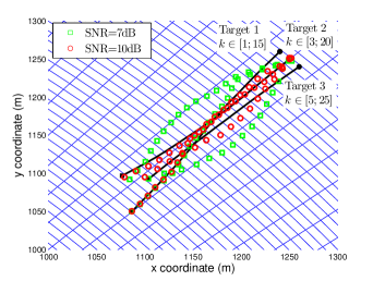
Figure 1: Simulated scenario and estimated trajectories. The radar is positioned at the Cartesian origin and there are $3$ closely spaced targets moving towards the origin.

Results in terms of the estimated number of targets and Optimal Sub-Pattern Assignment (OSPA) distance [51] are reported in Figs. 3(a)-3(b) for the case with $SNR=10dB$ and in Figs. 4(a)-4(b) for the more difficult case with $SNR=7dB$. Notice from Fig. 3(b) the increase in OSPA distance after $k=3$ and $k=5$, i.e. the instants at which new targets enter the scene, and then reduces in time thanks to the filter convergence. For the more difficult case with $SNR=7dB$, we notice in Fig. 4(b) a slower filter convergence and increasing OSPA distance also for $k=15$ and $k=20$, i.e. the instants at which targets disappear. This is due to the fact that for lower $SNR$ the tracker prefers to retain a “false” track for few steps rather then declaring a “dead” target too soon, as confirmed by the time behaviour of the average estimated number of targets in Fig. 4(a). Tuning of the survival probability $P_{S}$ can reduce this phenomenon. In practice, a perfect tuning of $P_{S}$ and of the birth probability $P_{B}$ require additional prior knowledge on the surveillance area. Overall, the results confirm the applicability of the proposed approach for challenging multi-target problems with closely spaced targets and low $SNR$.

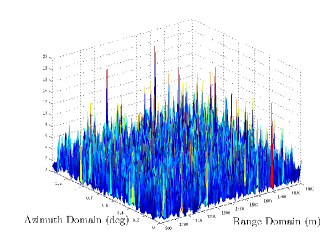
(a) $7dB$ for $k=8$: Targets at $(r=1.7km,b=0.78\deg)$

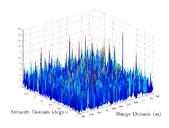
(b) $10dB$ for $k=8$: Targets at $(r=1.7km,b=0.78\deg)$

Figure 2: Snapshot of the simulated radar power returns for low $SNR$ and closely spaced targets.

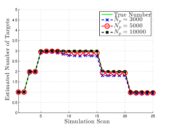
(a) Monte Carlo results: No. of Targets for $SNR=10dB$

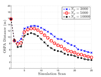
(b) Monte Carlo results: OSPA Distance for $SNR=10dB$

Figure 3: Monte Carlo results for the case $SNR=10dB$

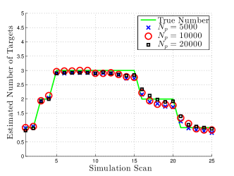
(a) Monte Carlo results: No. of Targets for $SNR=7dB$

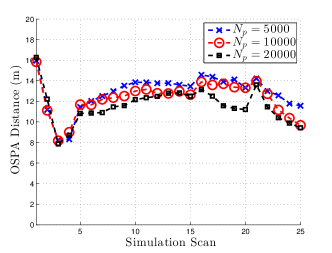
(b) Monte Carlo results: OSPA Distance for $SNR=7dB$

Figure 4: Monte Carlo results for the case $SNR=7dB$

VI Conclusions and Future Research

In this paper we discussed a general solution for multi-target tracking with superpositional measurements. The proposed approach aims at evaluating the multi-target Bayes filter using SMC methods. The critical enabling step was the definition of an efficient proposal distribution based on the Approximate CPHD filter for superpositional measurements. Numerical results confirmed the applicability to challenging multi-target tracking problems for closely spaced targets using radar measurements with low SNR. A large-scale application of this approach might not be possible due to worsening depletion problems in high dimensional state spaces. However, MCMC methods could be used to devise a particle implementation that can scale with an increasing number of targets. Furthermore, subdividing the targets into statistically non-interacting clusters and then processing the clusters separately could lead to satisfactory performance with reduced computational load. Finally, the capability of separating closely spaced targets for superpositional measurements, i.e. estimating the correct cardinality when there are unresolved targets, means the approach could also be used as an initialization block of cheaper trackers like the LMB [32] and Vo-Vo [31] filters. Specifically, parts of the radar superpositional measurement could be processed with the proposed approach to find the correct number of targets as well as there location, then thresholded measurements could be processed with the LMB/Vo-Vo tracker. This should lead to improved performance as the LMB/Vo-Vo tracker would be using a more informative prior distribution.

Francesco Papi received the Laurea degree in Control Engineering in 2007 and a Ph.D. degree in Computer Science and Control Engineering in 2011, both from the University of Firenze, Italy. In January 2011 he joined Thales Nederland B.V. in Hengelo, the Netherlands, as a Marie Curie Research Fellow. From January 2013 to April 2014 he was a Research Fellow at the Joint Research Centre, IPSC, European Commission, Ispra, Italy. He is currently Research Associate at the Department of Electrical and Computer Engineering, Curtin University, Perth, Australia. His research interests include linear and nonlinear Bayesian estimation, single and multi-sensor target tracking, and data fusion.

Du Yong Kim received his B. E. degree in Electrical and Electronics Engineering from Ajou University, Korea in 2005. He received his M. S. and Ph. D. degrees from the Gwangju Institute of Science and Technology, Korea in 2006 and 2011, respectively. As a Postdoctoral researcher he has worked on statistical signal processing and image processing at the Gwangju Institute of Science and Technology, 2011-2012, University of Western Australia, 2012-2014. He is currently working as a research associate at the Department of Electrical and Computer Engineering, Curtin University. His main research interests include Bayesian filtering theory and its applications to machine learning, computer vision, sensor networks and automatic control.

References

- [1] B. Balakumar, A. Sinha, T. Kirubarajan, and J. Reilly, “PHD filtering for tracking an unknown number of sources using an array of sensors,” in IEEE 13th Workshop on Statistical Signal Processing, 2005, pp. 43–48.
- [2] D. Angelosante, E. Biglieri, and M. Lops, “Multiuser detection in a dynamic environment: Joint user identification and parameter estimation,” in Proc. IEEE Int. Symp. Inf. Theory, Nice, France, June 2007, pp. 2071–2075.
- [3] O. Hlinka, O. Sluciak, F. Hlawatsch, P. Djuric, and M. Rupp, “Likelihood consensus and its application to distributed particle filtering,” IEEE Trans. Signal Processing, vol. 60, no. 8, pp. 4334–4349, 2012.
- [4] S. Nannuru, M. Coates, and R. Mahler, “Computationally-Tractable Approximate PHD and CPHD Filters for Superpositional Sensors,” Selected Topics in Signal Processing, IEEE Journal of, vol. 7, no. 3, pp. 410–420, June 2013.
- [5] D. Svensson, M. Ulmke, and L. Hammarstrand, “Multitarget Sensor Resolution Model and Joint Probabilistic Data Association,” IEEE Transactions on Aerospace and Electronic Systems, vol. 48, no. 4, pp. 3418–3434, 2012.
- [6] M. Beard, B.-T. Vo, and B.-N. Vo, “Bayesian Multi-target Tracking with Merged Measurements Using Labelled Random Finite Sets,” Signal Processing, IEEE Transactions on, vol. 63, no. 6, pp. 1433–1447, 2015.
- [7] S. Davey, M. Rutten, and N. Gordon, “Track-Before-Detect Techniques,” in Integrated Tracking, Classification, and Sensor Management: Theory and Applications, M. Mallick, V. Krishnamurty, and V. B.-N., Eds. Wiley/IEEE, 2012, ch. 8, pp. 311–361.
- [8] F. Papi, B.-N. Vo, B.-T. Vo, C. Fantacci, and M. Beard, “Generalized Labeled Multi-Bernoulli Approximation of Multi-Object Densities,” arXiv preprint, 2014, arXiv:1412.5294.
- [9] S. Blackman and R. Popoli, Design and Analysis of Modern Tracking Systems. Artech House, 1999.
- [10] R. Mahler, Statistical Multisource-Multitarget Information Fusion. Artech House, 2007.
- [11] Y. Bar-Shalom, P. K. Willett, and X. Tian, Tracking and Data Fusion: A Handbook of Algorithms. YBS Publishing, 2011.
- [12] G. Battistelli, L. Chisci, S. Morrocchi, F. Papi, A. Farina, and A. Graziano, “Robust multisensor multitarget tracker with application to passive multistatic radar tracking,” IEEE Transactions on Aerospace and Electronic Systems, vol. 48, no. 4, pp. 3450–3472, 2012.
- [13] S.-W. Joo and R. Chellappa, “A multiple-hypothesis approach for multiobject visual tracking,” IEEE Trans. Image Processing, vol. 16, no. 11, pp. 2849–2854, 2007.
- [14] M. Isard and J. MacCormick, “BraMBLe: a Bayesian multiple-blob tracker,” in Proc. Int. Conf. Computer Vision, 2001.
- [15] R. Hoseinnezhad, B.-N. Vo, and B.-T. Vo, “Visual Tracking in Background Subtracted Image Sequences via Multi-Bernoulli Filtering,” IEEE Trans. Signal Processing, vol. 61(2), pp. 392–397, 2013.
- [16] M. Montemerlo, S. Thrun, and B. Siciliano, FastSLAM: A Scalable Method for the Simultaneous Localization and Mapping Problem in Robotics. Springer, 2007.
- [17] C. Lee, D. Clark, and J. Salvi, “SLAM with dynamic targets via single-cluster PHD filtering,” IEEE Journal of Selected Topics in Signal Processing, vol. 7, no. 3, pp. 543–552., 2013.
- [18] H. Durrant-Whyte and T. Bailey, “Simultaneous localization and mapping: Part I,” IEEE Robotics and Automation Magazine, vol. 13, no. 2, pp. 99–110, 2006.
- [19] J. Mullane, B.-N. Vo, M. Adams, and B.-T. Vo, “A Random Finite Set Approach to Bayesian SLAM,” IEEE Trans. Robotics, vol. 27, no. 2, pp. 268–282, 2011.
- [20] G. Battistelli, L. Chisci, S. Morrocchi, F. Papi, A. Benavoli, A. Di Lallo, A. Farina, and A. Graziano, “Traffic intensity estimation via PHD filtering,” in European Radar Conference, 2008, pp. 340–343.
- [21] D. Meissner, S. Reuter, and K. Dietmayer, “Road user tracking at intersections using a multiple-model PHD filter,” in Intelligent Vehicles Symposium (IV), 2013 IEEE, 2013, pp. 377–382.
- [22] N. Ray and K. Ley, “Tracking leukocytes in vivo with shape and size constrained active,” Medical Imaging, vol. 21, no. 10, pp. 1222–1235, 2002.
- [23] I. Smal, K. Draegestein, and N. Galjart, “Particle Filtering for Multiple Object Tracking in Dynamic Fluorescence Microscopy Images Application to Microtubule Growth Analysis,” Medical Imaging, vol. 27, no. 6, 2008.
- [24] R. R. Juang, A. Levchenko, and P. Burlina, “Tracking cell motion using GM-PHD,” in IEEE Int. Symp. Biomedical Imaging, 2009, pp. 1154–1157.
- [25] R. Chatterjee, M. Ghosh, and A. S. Chowdhury, “Cell tracking in microscopic video using matching and linking of bipartite graphs,” Comput Methods Programs Biomed, vol. 112, no. 3, pp. 422–431, 2013.
- [26] S. Rezatofighi, S. Gould, B.-T. Vo, B.-N. Vo, K. Mele, and R. Hartley, “Multi-Target Tracking with Time-Varying Clutter Rate and Detection Profile: Application to Time-lapse Cell Microscopy Sequences,” IEEE Transactions on Medical Imaging, vol. PP, no. 99, pp. 1–1, 2015.
- [27] G. Battistelli, L. Chisci, F. Papi, A. Benavoli, A. Farina, and A. Graziano, “Optimal flow models for multiscan data association,” IEEE Transactions on Aerospace and Electronic Systems, vol. 47, no. 4, pp. 2405–2422, 2011.
- [28] R. Mahler and A. El-Fallah, “An approximate CPHD filter for superpositional sensors,” in Proc. SPIE, vol. 8392, 2012, pp. 83 920K–83 920K–11.
- [29] S. Nannuru and M. Coates, “Particle filter implementation of the multi-Bernoulli filter for superpositional sensors,” in IEEE 5th International Workshop on Computational Advances in Multi-Sensor Adaptive Processing (CAMSAP), December 2013, pp. 368–371.
- [30] ——, “Hybrid multi-Bernoulli CPHD filter for superpositional sensors,” in SPIE Defense + Security, I. S. for Optics and Photonics, Eds., June 2014, pp. 90 910D–90 910D.
- [31] B.-T. Vo and B.-N. Vo, “Labeled Random Finite Sets and Multi-Object Conjugate Priors,” IEEE Trans. Sig. Proc., vol. 61(13), pp. 3460–3475, 2013.
- [32] S. Reuter, B. Wilking, J. Wiest, M. Munz, and K. Dietmayer, “Real-Time Multi-Object Tracking using Random Finite Sets,” IEEE Trans. Aerospace and Electronic Systems, vol. 49, no. 4, pp. 2666–2678, 2013.
- [33] R. Mahler, Advances in Statistical Multisource-Multitarget Information Fusion. Artech House, 2014.
- [34] B.-N. Vo, B.-T. Vo, and D. Phung, “Labeled Random Finite Sets and the Bayes Multi-Target Tracking Filter,” IEEE Trans. Sig. Proc., vol. 62(24), pp. 6554–6567, 2014.
- [35] Y. Boers and J. N. Driessen, “Multitarget Particle Filter Track-Before-Detect application,” IEE Proc. on Radar, Sonar and Navigation, vol. 151, pp. 351–357, 2004.
- [36] R. Mahler, “Multi-target Bayes filtering via first-order multi-target moments,” IEEE Trans. Aerospace & Electronic Systems, vol. 39(4), pp. 1152–1178, 2003.
- [37] B.-N. Vo, S. Singh, and A. Doucet, “Sequential Monte Carlo methods for Multi-target filtering with Random Finite Sets,” IEEE Transactions on Aerospace and Electronic Systems, vol. 41, no. 4, pp. 1224–1245, 2005.
- [38] A. Doucet, S. J. Godsill, and C. Andrieu, “On sequential monte carlo sampling methods for bayesian filtering,” Stat. Comp., vol. 10, pp. 197–208, 2000.
- [39] T. Vu, B.-N. Vo, and R. J. Evans, “A Particle Marginal Metropolis-Hastings Multi-target Tracker,” IEEE Trans. Signal Processing, vol. 62, no. 15, pp. 3953 – 3964, 2014.
- [40] C. Andrieu, A. Doucet, and R. Holenstein, “Particle Markov Chain Monte Carlo methods,” Journal of the Royal Statistical Society: Series B, vol. 72(3), pp. 269–342, 2010.
- [41] R. Mahler, “PHD filters of higher order in target number,” IEEE Trans. Aerospace & Electronic Systems, vol. 43(3), pp. 1523–1543, July 2007.
- [42] B.-N. Vo, B.-N. Vo, and A. Cantoni, “Analytic implementations of the Cardinalized Probability Hypothesis Density filter,” IEEE Trans. Signal Processing, vol. 55, no. 7, pp. 3553–3567, 2007.
- [43] S. Reuter, B.-T. Vo, B.-N. Vo, and K. Dietmayer, “The labelled multi-Bernoulli filter,” IEEE Trans. Signal Processing, vol. 62(12), pp. 3246–3260, 2014.
- [44] Y. Boers and H. Driessen, “The mixed labeling problem in multi target particle filtering,” in 10th International Conference on Information Fusion, 2007, pp. 1–7.
- [45] W.-K. Ma, B.-N. Vo, S. Singh, and A. Baddeley, “Tracking an unknown and time varying number of speakers using TDOA measurements: A Random Finite Set Approach,” IEEE Trans Signal Processing, vol. 54, no. 9, pp. 3291–3304, 2006.
- [46] B. Ristic and B.-N. Vo, “Sensor Control for Multi-Object State-Space Estimation Using Random Finite Sets,” Automatica, vol. 46, no. 11, pp. 1812–1818, 2010.
- [47] A. Gray, “Bringing Tractability to Generalized N-Body Problems in Statistical and Scientific Computing,” Ph.D. dissertation, Carnegie Mellon University, 2003.
- [48] M. Klaas, M. Briers, N. de Freitas, A. Doucet, S. Maskell, and D. Lang, “Fast Particle Smoothing: If I Had a Million Particles,” Proc. of the Int. Conference on Machine Learning, Pittsburg, PA, USA 2006.
- [49] F. Papi, M. Bocquel, M. Podt, and Y. Boers, “Fixed-Lag Smoothing for Bayes Optimal Knowledge Exploitation in Target Tracking,” Signal Processing, IEEE Transactions on, vol. 62, no. 12, pp. 3143–3152, June 2014.
- [50] M. Bocquel, F. Papi, M. Podt, and Y. Driessen, “Multitarget Tracking With Multiscan Knowledge Exploitation Using Sequential MCMC Sampling,” IEEE J. Selected Topics in Sig. Proc., vol. 7(3), pp. 532–542, 2013.
- [51] D. Schuhmacher, B.-T. Vo, and B.-N. Vo, “A consistent metric for performance evaluation of multi-object filters,” IEEE Trans. Signal Processing, vol. 56, no. 8, pp. 3447–3457, Aug. 2008.