APEX-CHAMP⁺ high-$J$ CO observations of
low–mass young stellar objects

Abstract

Context. During the embedded stage of star formation, bipolar molecular outflows and UV radiation from the protostar are important feedback processes. Both processes reflect the accretion onto the forming star and affect subsequent collapse or fragmentation of the cloud.

Aims. Our aim is to quantify the feedback, mechanical and radiative, for a large sample of low-mass sources in a consistent manner. The outflow activity is compared to radiative feedback in the form of UV heating by the accreting protostar to search for correlations and evolutionary trends.

Methods. Large-scale maps of 26 young stellar objects, which are part of the Herschel WISH key program are obtained using the CHAMP⁺ instrument on the Atacama Pathfinder EXperiment (¹²CO and ¹³CO 6–5; $E_{\rm up}$$\sim$100 K), and the HARP-B instrument on the James Clerk Maxwell Telescope (¹²CO and ¹³CO 3–2; $E_{\rm up}$$\sim$30 K). The maps have high spatial resolution, particularly the CO 6–5 maps taken with a 9$\arcsec$ beam, resolving the morphology of the outflows. The maps are used to determine outflow parameters and the results are compared with higher-$J$ CO lines obtained with Herschel. Envelope models are used to quantify the amount of UV-heated gas and its temperature from ¹³CO 6–5 observations.

Results. All sources in our sample show outflow activity, with the spatial extent decreasing from the Class 0 to the Class I stage. Consistent with previous studies, the outflow force, $F_{\rm CO}$, is larger for Class 0 sources than for Class I sources, even if their luminosities are comparable. The outflowing gas typically extends to much greater distances than the power-law envelope and therefore influences the surrounding cloud material directly. Comparison of the CO 6–5 results with HIFI H₂O and PACS high-$J$ CO lines, both tracing currently shocked gas, shows that the two components are linked, even though the transitions do not probe the same gas. The link does not extend down to CO 3–2. The conclusion is that CO 6–5 depends on the shock characteristics (density and velocity), whereas CO 3–2 is more sensitive to conditions in the surrounding environment (density). The radiative feedback is responsible for increasing the gas temperature by a factor of two, up to 30–50 K, on scales of a few thousand AU, particularly along the direction of the outflow. The mass of the UV heated gas exceeds the mass contained in the entrained outflow in the inner $\sim$3000 AU and is therefore at least as important on small scales.

1 Introduction

During the early phases of star-formation, material surrounding the newly forming star accretes onto the protostar. At the same time, winds or jets are launched at supersonic speeds from the star-disk system, which sweep up surrounding envelope material in large bipolar outflows. The material is accelerated and pushed to distances of several tens of thousands of AU, and these outflows play a pivotal role in the physics and chemistry of the star-forming cores (Snell et al. 1980; Goldsmith et al. 1984; Lada 1987; Greene et al. 1994; Bachiller & Tafalla 1999; Arce & Sargent 2006; Tafalla et al. 2013). The youngest protostars have highly collimated outflows driven by jets, whereas at later stages wide-angle winds drive less collimated outflows. However, there is still not a general consensus to explain the launching mechanisms and nature of these outflows (Arce et al. 2007; Frank et al. 2014).

The goal of this paper is to investigate how the outflow activity varies with evolution and how this compares with other measures of the accretion processes for low-mass sources. The outflows reflect the integrated activity over the entire lifetime of the protostar, which could be the result of multiple accretion and ejection events. It is important to distinguish this probe from the current accretion rate, as reflected for example in the luminosity of the source, in order to understand the accretion history. The well-known “luminosity problem” in low-mass star-formation indicates that protostars are underluminous compared to theoretical models (Kenyon et al. 1990; Evans et al. 2009; Enoch et al. 2009; Dunham et al. 2010, 2013). One of the possible resolutions to this problem is that of “episodic accretion”, in which the star builds up through short bursts of rapid accretion over long periods of time rather than continuous steady-state accretion. An accurate and consistent quantification of outflow properties, such as the outflow force and mass, is essential for addressing this problem.

Outflows have been observed in CO emission in the last few decades towards many sources, but those observations were mainly done via lower-$J$ CO rotational transitions ($J_{\rm u}$$\leq$3), which probe colder swept-up or entrained gas ($T$$\sim$50–100 K) (e.g., Bachiller et al. 1990; Blake et al. 1995; Bontemps et al. 1996; Tafalla et al. 2000; Curtis et al. 2010, and many others). One of the most important parameters that is used for the evolutionary studies of star formation is the “outflow force”, which is known as the strength of an outflow and defined similar to any $r^{-2}$-type force. These studies conclude that the outflow force correlates well with bolometric luminosity, $L_{\rm bol}$, a correlation which holds over several orders of magnitude. Furthermore, the outflow force from Class 0 sources is stronger than for Class I sources, indicating an evolutionary trend. The correlations, however, often show some degree of scatter, typically more than an order of magnitude in $F_{\rm CO}$ for any value of $L_{\rm bol}$. Some of the uncertainties in these studies include the opacity in the line wings, the adopted inclination angle and cloud contamination at low outflow velocities (e.g., van der Marel et al. 2013). Comparison with other outflow tracers such as water recently observed with the Herschel Space Observatory is further complicated because the various studies use different analysis methods to derive outflow parameters from low-$J$ CO maps. One of the goals of this paper is to provide a consistent set of outflow parameters determined by the same method using data from the same telescopes for comparison with the Herschel lines.

Recently, the importance of radiative feedback from low-mass protostars on all scales of star formation has been acknowledged. On cloud scales ($>$10⁴ AU) the feedback sets the efficiency at which cores fragment from the cloud and form stars (Offner et al. 2009, 2010; Hansen et al. 2012) because the Jeans length scales as $T^{0.5}$. Simulations including radiative feedback and radiative transfer reproduce the observed initial mass function (IMF) better than models without these effects included (Offner et al. 2009). On the scales of individual cores ($<$3000 AU), the radiative feedback suppresses the fragmentation into multiple systems and serves to stabilize the protostellar disk (Offner et al. 2010). Thus, quantifying observationally the temperature changes as a function of position from the protostar are important steps toward more accurate models of star formation. The first observational evidence of heating of the gas around low-mass protostars on scales of $\sim$1000 AU by UV radiation escaping through the outflow cavities dates back to Spaans et al. (1995) based on strong narrow ¹³CO 6–5 lines, and has since been demonstrated and quantified for a few more sources by van Kempen et al. (2009b); Yıldız et al. (2012); Visser et al. (2012). We note that this UV-heated gas is warm gas with temperatures higher than that of the dust, and is thus in excess of warm material in the envelope that has been heated by the protostellar luminosity, where the gas temperature is equal to the dust temperature. Although UV heating toward photo-dissociation regions (PDRs) is readily traced by emission from polycyclic aromatic hydrocarbons (PAHs), the PAH abundance toward embedded protostars is too low for them to be used as a tool in this context (Geers et al. 2009). Here we investigate the importance of radiative feedback for a much larger sample of low-mass sources and compare the gas temperatures and involved mass with that of the outflows.

Tracing warm gas ($T$$\gtrsim$30 K) in the envelope or in the surroundings requires observations of higher-$J$ transitions of CO, e.g., $J_{\rm u}$$\geq$5, for which ground-based telescopes demand excellent weather conditions on dry observing sites. The CHAMP⁺ instrument, mounted on the Atacama Pathfinder EXperiment (APEX) telescope is ideally suited to observe higher-$J$ CO transitions and efficiently map extended sources. The broad line wings of CO 6–5 ($E_{\rm u}/k$=115 K) suffer less from opacity effects than CO 3–2 ($E_{\rm u}/k$=33 K) (van Kempen et al. 2009a; Yıldız et al. 2012). Moreover, the ambient cloud contribution is smaller for these higher-$J$ transitions, except close to the source position, where the dense protostellar envelope may still contribute. Even higher-$J$ CO lines up to $J_{\rm u}$$\sim$50 were routinely observed with the Herschel (Pilbratt et al. 2010) and provide information on the shocked gas in the Herschel beam (Herczeg et al. 2012; Goicoechea et al. 2012; Benedettini et al. 2012; Manoj et al. 2013; Green et al. 2013; Nisini et al. 2013; Karska et al. 2013). This currently shocked gas is different from that observed in low-$J$ CO transitions, as is evident from their different spatial distributions (Tafalla et al. 2013; Santangelo et al. 2013).

In this paper, we present an APEX-CHAMP⁺ survey of 26 low-mass young stellar objects (YSOs), which were mapped in CO $J$=6–5 and isotopologues in order to trace their outflow activity, following van Kempen et al. (2009a, b) and Yıldız et al. (2012), papers I, II and III in this series, on individual or more limited samples of sources. These data complement our earlier surveys at lower frequency of CO and other molecules with the James Clerk Maxwell Telescope (JCMT) and APEX (e.g., Jørgensen et al. 2002, 2004; van Kempen et al. 2009c). The same sources are covered in the Herschel key project, “Water in star-forming regions with Herschel” (WISH; van Dishoeck et al. 2011), which has observed H₂O and selected high-$J$ CO lines with HIFI and PACS instruments. Many of the sources are also included in the “Dust, Ice and Gas in Time” program (DIGIT; PI: N. Evans; Green et al. 2013), which has obtained full PACS spectral scans. The results obtained from the ¹²CO maps are complemented by ¹³CO 6–5 data of the same sources, with the narrower ¹³CO 6–5 lines probing the UV photon-heated gas.

The YSOs in our sample cover both the deeply embedded Class 0 stage as well as the less embedded Class I stage (André et al. 2000; Robitaille et al. 2006). Physical models of the dust temperature and density structure of the envelopes have been developed for all sources by Kristensen et al. (2012) through spherically symmetric radiative transfer models of the continuum emission. The full data set covering many sources, together with the envelope models, allows us to address important characteristics of YSOs through the evolution from Class 0 to Class I in a more consistent manner. These characteristics can be inferred from their different morphologies, outflow forces, envelope masses, etc. and eventually be compared with evolutionary models. The study presented here is also complementary to that of Yıldız et al. (2013), where only the source position was studied with spectrally resolved CO line profiles from $J$=2–1 to 10–9 ($E_{\rm up}$$\sim$300 K), and trends with evolution were examined.

The outline of the paper is as follows. In Section 2, the observations and the telescopes where the data have been obtained are described. In Section 3, physical parameters obtained from molecular outflows are given and the UV heated gas component is identified. In Sect. 4, these results are discussed, and conclusions from this work are presented in Sect. 5.

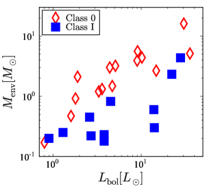
Figure 1: Envelope mass,$M_{\rm env}$, vs bolometric luminosity, $L_{\rm bol}$, for the surveyed sources. Red diamonds and blue squares indicate Class 0 and Class I sources, respectively.

2 Sample and observations

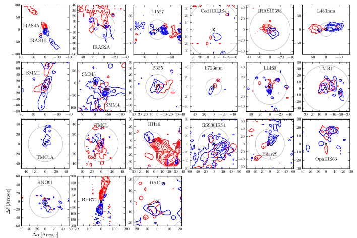
Figure 2: Overview of the outflows traced by the ¹²CO 6–5 observations with the APEX-CHAMP⁺ instrument. Contour levels are given in Table 11 and the source is located at (0,0) in each map, with the exception of the maps of NGC 1333-IRAS 4A and IRAS 4B, and Ser-SMM3 and Ser-SMM4, which are located in the same maps and centered on NGC 1333-IRAS 4A and Ser-SMM3, respectively. The circle in each plot corresponds to a region of 5000 AU radius at the distance of each source. Velocity ranges over which the integration was done are provided in Table 11.

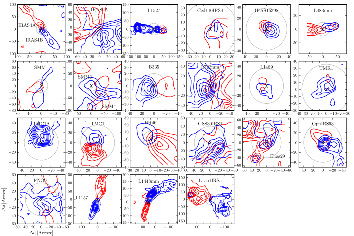
Figure 3: Overview of the entire set of outflows traced by the ¹²CO 3–2 observations with the JCMT and APEX. Contour levels are given in Table 11 and the source is located at (0,0) in each map, with the exception of the maps of NGC 1333-IRAS 4A and NGC 1333-IRAS 4B, and Ser-SMM3 and Ser-SMM4, which are located in the same maps and centered on NGC 1333-IRAS 4A and Ser-SMM3, respectively. The circle in each plot corresponds to a region of 5000 AU radius at the distance of each source. Velocity ranges over which the integration was done are provided in Table 11.

2.1 Sample

The sample selection criteria with the coordinates and other basic information of the source list are presented in van Dishoeck et al. (2011) with updates in Kristensen et al. (2012), and is the same as the sample presented in Yıldız et al. (2013). It consists of 15 Class 0 and 11 Class I embedded protostellar sources located in the Perseus, Ophiuchus, Taurus, Chamaeleon, and Serpens molecular clouds. The average distance is 200 pc, with a maximum distance of 450 pc.

Figure 1 presents the envelope mass ($M_{\rm env}$) as a function of bolometric luminosity ($L_{\rm bol}$) for all sources. The parameters are taken from the continuum radiative transfer modeling by Kristensen et al. (2012) based on fits of the spectral energy distributions (SEDs) including new Herschel-PACS fluxes, as well as the spatial extent of the envelopes observed at submillimeter wavelengths. The envelope mass is measured either at the $T_{\rm dust}$=10 K radius or at the $n$=10⁴ cm^-3 radius, depending on which is smaller. Class 0 and Class I sources are well separated in the diagram, with the Class 0 sources having higher envelope masses. This type of correlation diagram has been put forward by Saraceno et al. (1996) and subsequently used as an evolutionary diagram for embedded YSOs with lower envelope masses representing later stages (e.g., Bontemps et al. 1996; Hogerheijde et al. 1998; Hatchell et al. 2007). In our sample, envelope masses range from 0.04 M_⊙ (Elias 29) to 16 M_⊙ (Ser-SMM1) and the luminosities range from 0.8 L_⊙ (Ced110 IRS4) to 35.7 L_⊙ (NGC 1333-IRAS 2A). The large range of masses and luminosities makes the sample well suited for studying trends with various source parameters. The range of luminosities studied is similar to that of Bontemps et al. (1996), $\sim$0.5 to 15 L_⊙, but our sample is more weighted toward higher luminosities and earlier stages.

2.2 Observations

Molecular line observations of CO in the $J$=6–5 transitions were done with the 12-m submillimeter Atacama Pathfinder EXperiment, APEX (Güsten et al. 2008) at Llano de Chajnantor in Chile, whereas the $J$=3–2 transition was primarily observed at the 15-m James Clerk Maxwell Telescope, JCMT at Mauna Kea, Hawaii.

APEX: ¹²CO and ¹³CO 6–5 maps of the survey were obtained with the CHAMP⁺ instrument on APEX between June 2007 and September 2012. The CHAMP⁺ instrument consists of two heterodyne receiver arrays, each with seven pixel detector elements for simultaneous operations in the 620–720 GHz and 780–950 GHz frequency ranges (Kasemann et al. 2006; Güsten et al. 2008). The observational procedures are explained in detail in van Kempen et al. (2009a, b, c) and Yıldız et al. (2012). Simultaneous observations were done with the following settings of the lower and higher frequency bands: ¹²CO 6–5 with ¹²CO 7–6; ¹³CO 6–5 with [C i] 2–1. ¹²CO maps cover the entire outflow extent with a few exceptions (L1527, Ced110 IRS4, and L1551-IRS5), whereas ¹³CO maps cover only a $\sim$100^′′$\times$100^′′ region around the central source position. L1157 is part of the WISH survey, but because it is not accessible from APEX (dec = $+$68°), no CO 6–5 data are presented.

The APEX beam size is $\sim$9^′′ ($\sim$1800 AU for a source at 200 pc) at 691 GHz. The observations were done using position-switching toward an emission-free reference position. The CHAMP⁺ instrument uses the Fast Fourier Transform Spectrometer (FFTS) backend (Klein et al. 2006) for all seven pixels with a resolution of 0.183 MHz (0.079 km s^-1 at 691 GHz). The $rms$ at the source position is listed in Yıldız et al. (2013) for the CO 6–5 and ¹³CO 6–5 observations and is typically 0.3–0.5 K for the former and 0.1–0.3 K for the latter, both in 0.2 km s^-1 channels. The rms increases near the map edges where the effective integration time per beam was significantly smaller than in the central parts; near the edges the rms may be twice as high. Apart from the high-$J$ CO observations, some of the 3–2 line observations were also conducted with APEX for a few southern sources, e.g., DK Cha, Ced110 IRS4, and HH 46 (van Kempen et al. 2009c).

JCMT: Fully sampled jiggle maps of ¹²CO and ¹³CO 3–2 were obtained using the HARP-B instrument mounted on the JCMT. HARP-B consists of 16 SIS detectors with 4$\times$4 pixel elements of 15^′′ each at 30^′′ separation. Most of the maps were obtained through our own dedicated proposals, with a subset obtained from the JCMT public archive.

The data were acquired on the $T_{\rm A}^{*}$ antenna temperature scale and were converted to main-beam brightness temperatures $T_{\rm MB}$=$T_{\rm A}^{*}/\eta_{\rm MB}$ using the beam efficiencies ($\eta_{\rm MB}$). The CHAMP⁺ beam efficiencies were taken from the CHAMP⁺ website and forward efficiencies are 0.95 in all observations. The various beam efficiencies are all given in Yıldız et al. (2013, their Appendix C) and are typically $\sim$0.5. The JCMT beam efficiencies were taken from the JCMT Efficiencies Database, and 0.63 is used for all HARP-B observations. Calibration errors are estimated to be $\sim$20% for both telescopes. Typical $rms$ noise levels of the $J$=3–2 data are from 0.05 K to 0.1 K in 0.2 km s^-1 channels.

For the data reduction and analysis, the “Continuum and Line Analysis Single Dish Software”, CLASS program, which is part of the GILDAS software, is used. In particular, linear baselines were subtracted from all spectra. ¹²CO and ¹³CO 6–5 and 3–2 line profiles of the central source positions of all the sources in the sample are presented in Yıldız et al. (2013).

2.3 ¹²CO maps

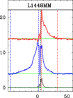
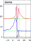
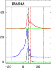
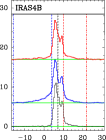
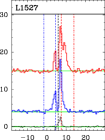
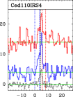
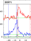
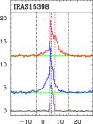
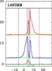
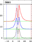
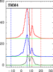
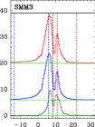
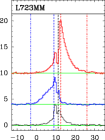
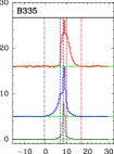
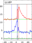
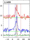
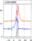
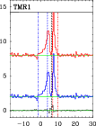
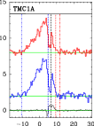
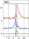
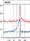
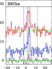
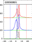
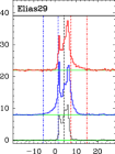
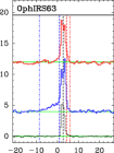
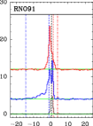
Figure 13: CO 3–2 spectra with selected integration limits indicated, except for Ced110 IRS4, BHR71, and DK Cha where CO 6–5 was used. Each panel presents these limits for each source. The black spectrum at the bottom is taken from a clean position representative for the envelope emission. The blue spectrum at the middle is the representative spectrum from the blue outflow lobe, and red spectrum at the top is the representative spectrum from the red outflow lobe. Each panel shows five vertical lines, these are $V_{\rm LSR}$ (black dashed line), $V_{\rm out,blue}$ (dot-dash blue line), $V_{\rm in,blue}$ (dashed blue line), $V_{\rm in,red}$ (dashed red line), and $V_{\rm out,red}$ (dot-dash red line).

All spectra are binned to a 0.5 km s^-1 velocity resolution for analyzing the outflows. The intensities of the blue and red outflow lobes are calculated by integrating the blue and red emission in each of the spectra separately, where the integration limits are carefully selected for each source by using the 0.2 km s^-1 resolution CO 3–2 or 6–5 spectra if the former is not available (see Fig. 13). First, the inner velocity limit, $V_{\rm in}$, closest to the source velocity is determined by selecting a spatial region not associated with the outflow. The ¹²COspectra in this region are averaged to determine the narrow line emission coming from the envelope and surrounding cloud, and $V_{\rm in}$ is estimated from the width of the quiescent emission (see Fig. 13 in the Appendix). Second, the outer velocity limits $V_{\rm out}$ are determined from the highest $S/N$ spectrum inside each of the blue and red outflow lobes. The outer velocity limits are selected as the velocity where the emission in the spectrum goes down to the 1$\sigma$ limit for the first time. It therefore excludes extremely high velocity or ‘bullet’ emission which is seen for a few sources. The blue- and red-shifted integrated intensity is measured by integrating over these velocity limits across the entire map, but excluding any extremely high velocity (EHV) or “bullet” emission.

2.3.1 Outflow velocity

The maximum outflow velocity, $V_{\rm max}$ is defined as $\lvert$$V_{\rm out}$–$V_{\rm LSR}$$\lvert$, the total velocity extent measured relative to the source velocity. In order to estimate $V_{\rm max}$, representative spectra from the blue and red outflow lobes observed in CO 3–2 are selected separately, and $V_{\rm out}$ is measured as described above. The differences between the velocity, where the emission reaches 1$\sigma$ level ($V_{\rm out}$) with $V_{\rm LSR}$ are taken as the global $V_{\rm max}$ values for the corresponding blue and red-shifted lobes (Cabrit & Bertout 1992).

Two issues arise when determining $V_{\rm max}$ (e.g., van der Marel et al. 2013; Dunham et al. 2014): First, $V_{\rm max}$ is a function of the $rms$ noise level and generally decreases with increasing $rms$. For noisy data, $V_{\rm max}$ may be underestimated compared to its true value. For this reason, the 3–2 lines are chosen to determine $V_{\rm max}$ because of their higher $S/N$ than the 6–5 lines. Second, if the outflow lobes are inclined, $V_{\rm max}$ suffers from projection effects. Both effects will increase the value of $V_{\rm max}$ if properly taken into account.

Concerning the second issue, the inclination is difficult to estimate from these data alone; proper-motion studies along with radial velocities are required to obtain an accurate estimate of the inclination. Alternatively, the velocity structure may be modeled assuming some distribution of material, e.g., a wind-driven shell with a Hubble-like flow (Lee et al. 2000), where the inclination then enters as a free parameter. It is defined as the angle between the outflow direction and the line of sight (Cabrit & Bertout 1990, $i$=0° is pole on). Small radial velocities are expected for outflows which lie in the plane of the sky. Therefore a correction factor for inclination $c_{i}$ is applied in the calculations. In Table 7, the correction factors from Downes & Cabrit (2007) are tabulated; these correction factors come from detailed outflow modeling and synthetic observations of the model results. Moreover, we note that these correction factors include correction for missing mass within $\pm$ 2 km s^-1 from the source velocity. The correction factors have been applied to the outflow rate, force and luminosity as listed in Tables 8 and 9. The velocity, as a measured parameter, is not corrected for inclination. The inclination angles are estimated from the outflow maps as follows: if the outflow lobes are overlapping, the outflow is likely very inclined. If the outflow shows low-velocity line wings but a large extent on the sky, the inclination is very likely low. In this way each outflow is classified individually, and divided into inclination bins at 10$\degr$, 30$\degr$, 50$\degr$, and 70$\degr$. Our estimates are listed in Tables 8 and 9, and are consistent with the literature where available (Cabrit & Bertout 1992; Gueth et al. 1996; Bourke et al. 1997; Hogerheijde et al. 1997; Micono et al. 1998; Brown & Chandler 1999; Lommen et al. 2008; Tobin et al. 2008; van Kempen et al. 2009b), except for IRAS 15398 for which we find a larger inclination than van Kempen et al. (2009c). Our inclination of IRAS 15398 is consistent with newer values from (Oya et al. 2014). Although the method for determining the outflow inclinations is subjective, the inclinations agree with literature values where available, which lends some credibility to the method, and we estimate that the uncertainty is 30°. That is, the correction introduces a potential systematic error of up to a factor of 2 in the outflow parameters.

Table 1: Inclination correction factors.

$i$($\degr$)	10	30	50	70
$c_{i}$	1.2	2.8	4.4	7.1

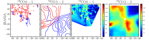
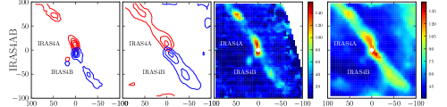
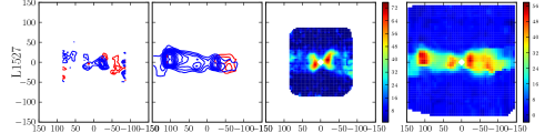
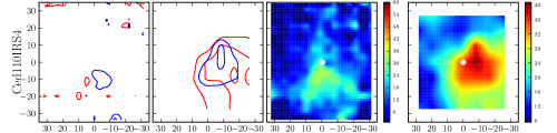
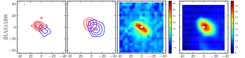
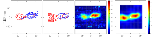
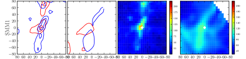
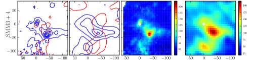
Figure 14: Each row contains contour and integrated intensity maps (in K km s^-1) of sources in ¹²CO 6–5 and 3–2. The contour levels and integration limits are given in Table 11 and integration limits shown in Fig. 13. The color images show all emission integrated from $V_{\rm out,red}$ to $V_{\rm out,blue}$, including any minor cloud contribution.

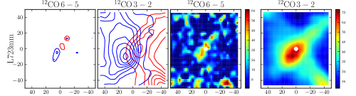
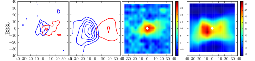
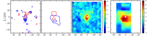
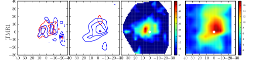
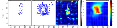
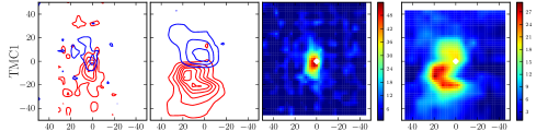
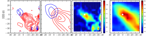
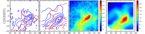
Figure 15: Caption is same as for Fig. 14.

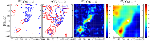
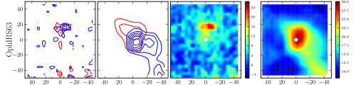
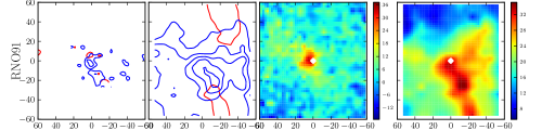
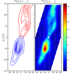
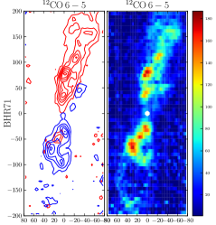
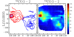
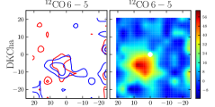
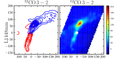
Figure 16: Caption is same as for Fig. 14.

The resulting maps of all sources are presented in Figs. 2 and 3 for ¹²CO 6–5 and 3–2, respectively, where blue and red contours show the blue- and red-shifted outflow lobes, respectively. The velocity limits are summarized in Table 11 in the Appendix. A few maps cover only the central $\sim$2′$\times$2′, specifically the three Class 0 sources NGC 1333-IRAS 2A, L723mm, L1527, and the two Class I sources Elias 29 and L1551-IRS5. Source-by-source outflow and intensity maps obtained from the CO 6–5 and 3–2 data are presented in Figs. 14–16 in the On-line Appendix.

2.4 ¹³CO maps

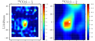
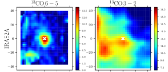
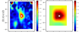
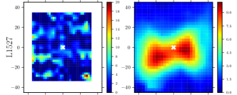
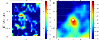
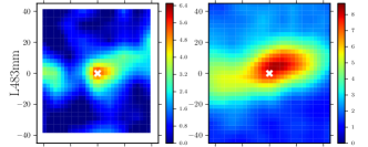
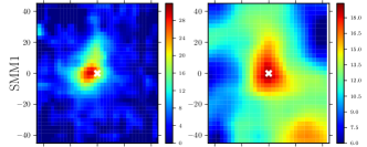
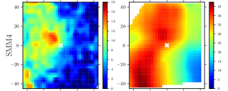
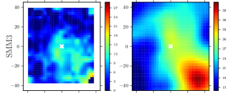
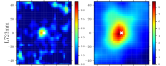
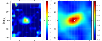
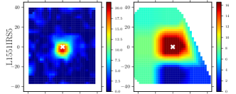
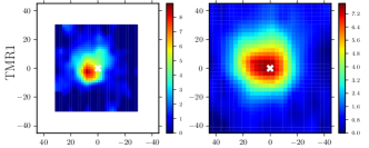
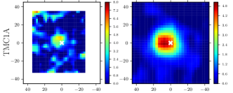
Figure 17: ¹³CO 6–5 and 3–2 integrated intensity maps of the sources (in K km s^-1).

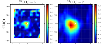
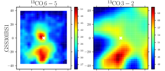
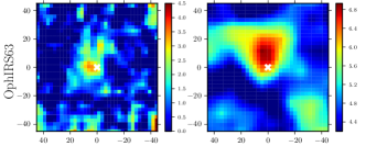
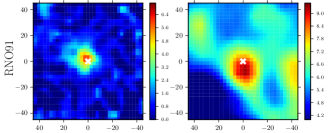
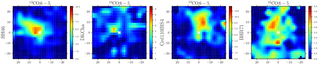
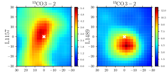
Figure 18: Caption is same as for Fig. 17.

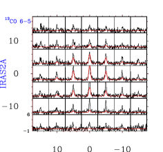
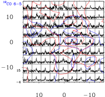
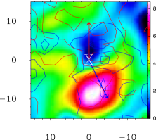
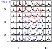
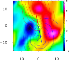
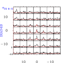
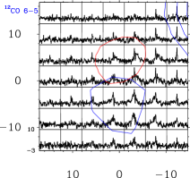
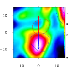
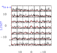
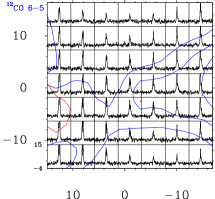
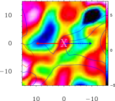
Figure 20: 7$\times$7 pixel fully sampled maps are extracted toward the central positions of the sources in ¹³CO 6–5 (left) and in ¹²CO 6–5 (middle) transitions. The axes represent the equatorial offsets ($\Delta$$\alpha$, $\Delta$$\delta$) in arcsec. The main beam temperature intensity scale of each box are shown in the y-axes of the bottom-left box in Kelvins. The velocity range in each box is $\pm$8 km s^-1 for the ¹³CO spectra, and $\pm$25 km s^-1 for the ¹²CO spectra. The red lines in the left-hand panels are the ¹³CO 6–5 model line intensities for the passively heated envelope. The excess emission in the observations compared with these model profiles corresponds to the UV-heated gas and is shown as an image in the right panel with the intensity scale in K km s^-1. The middle and right panels contain the red and blue outflow lobes with the contour levels given in Table 11. The blue and red arrows in the right-hand panels show the direction of the outflow lobes.

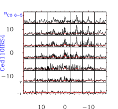
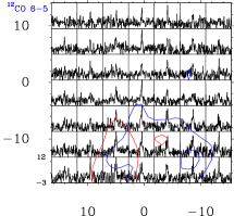
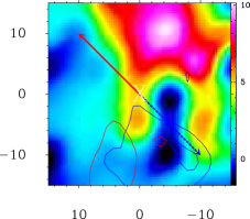
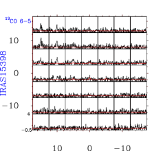
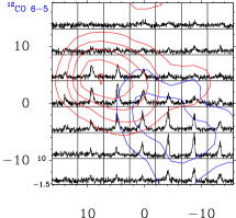
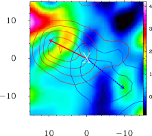
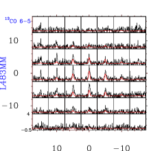
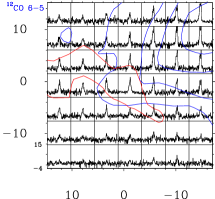
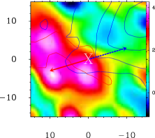
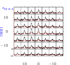
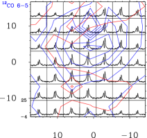
Figure 21: Same as Fig. 20.

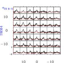
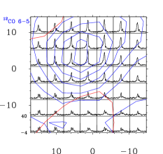
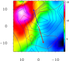
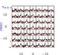
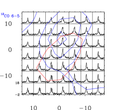
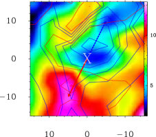
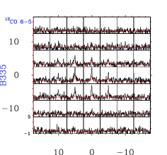
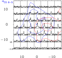
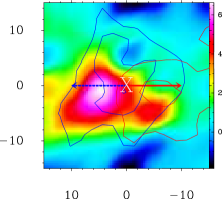
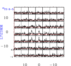
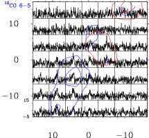
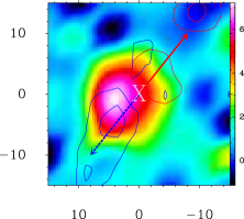
Figure 22: Same as Fig. 20.

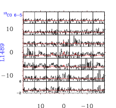
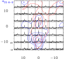
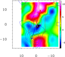
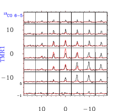
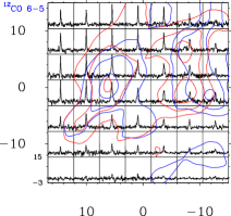
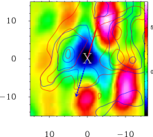
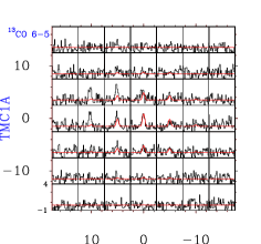
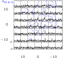
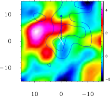
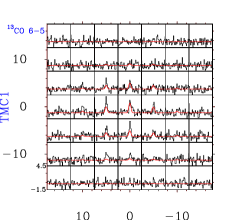
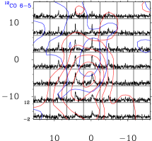
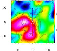
Figure 23: Same as Fig. 20.

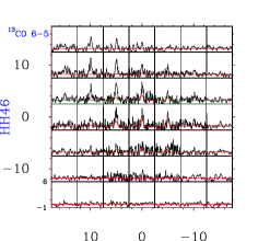
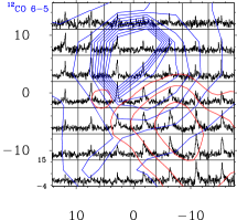
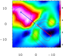
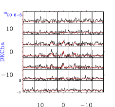
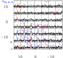
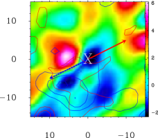
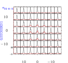
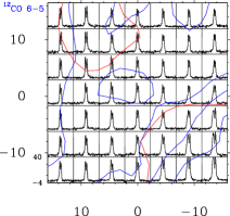
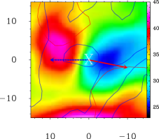
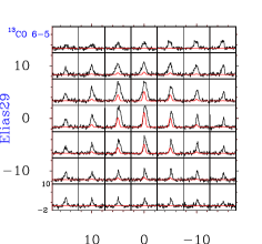
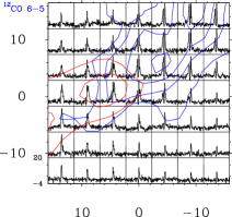
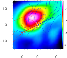
Figure 24: Same as Fig. 20.

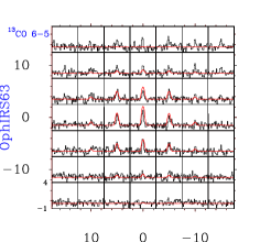
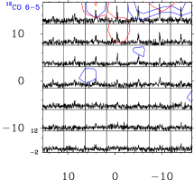
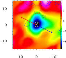
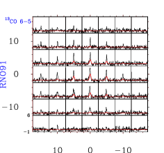
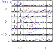
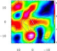
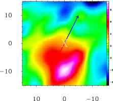
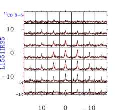
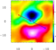
Figure 25: Same as Fig. 20. ¹²CO 6–5 transitions were not observed for L1448MM and L1551 IRS5 in our observing campaign, therefore left blank.

The ¹³CO 6–5 and 3–2 transitions were mapped around the central $\sim$1′$\times$1′ region, corresponding to typically $\sim$10⁴ AU $\times$ 10⁴ AU. The total integrated intensity is measured for all the sources and presented in Table C.1-26 of Yıldız et al. (2013) for the source positions. All maps are presented as contour maps in Figs. 17 and 18 and as spectral maps in Figs. 20-25 in the Appendix.

3 Results

3.1 Outflow morphology

All sources show strong outflow activity in both CO transitions, $J$=6–5 and 3–2, as is evident from both the maps and spectra (Figs. 2, 3, and Figs. 13–16). The advantage of the CO 6–5 maps is that they have higher spatial resolution by a factor of 2 than the CO 3–2 maps. On the other hand, the CO 3–2 maps have the advantage of higher $S/N$ than the CO 6–5 maps by typically a factor of 4 in main beam temperature.

Most sources show a clear blue-red bipolar structure. In a few cases only one lobe is observed. Specific examples are TMC1A, which shows no red-shifted outflow lobe, and HH 46, which has only a very small blue-shifted outflow lobe. One explanation is that these sources are at the edge of the cloud and that there is no cloud material to run into (van Kempen et al. 2009b). For L723mm, NGC 1333-IRAS 2A and BHR71, two outflows are driven by two independent protostars (Lee et al. 2002; Parise et al. 2006; Codella et al. 2014) and both outflows are detected in our CO 3–2 maps. In CO 6–5, only one outflow shows up toward L723mm and NGC 1333-IRAS 2A, whereas both outflows are seen toward BHR71.

Visual inspection shows that the Class 0 outflows are more collimated than their Class I counterparts as expected (e.g., Arce et al. 2007). The length of the outflows can be quantified for most of the sources. $R_{\rm CO}$ is defined as the total outflow extent assuming that the outflows are fully covered in the map. $R_{\rm CO}$ is measured separately for the blue and red outflow lobes as the projected size, with sometimes significantly different values. $R_{\rm CO}$ as measured from CO 6–5 is applied to CO 3–2 in the cases where the CO 6–5 maps are larger than their 3–2 counterparts. Toward some sources, e.g., DK Cha and NGC 1333-IRAS 4B, the blue and red outflow lobes overlap, likely because the outflows are observed nearly pole on. In other cases the outflow lobes cannot be properly isolated from nearby neighboring outflow lobes. Such a confusion is most pronounced in Ophiuchus (e.g., GSS30-IRS1). In those cases, $R_{\rm CO}$ could not be properly estimated and the estimated value is a lower limit. Figure 4 shows a histogram of total $R_{\rm CO}$ for Class 0 and I sources. Class 0 sources show a nearly flat distribution across the measured range of extents, whereas few Class I sources show large outflows (L1551 is a notable exception). In Fig. 5, $R_{\rm CO}$ is plotted against $R_{\rm 10K}$, the radius of the modeled envelope within a 10 K radius. The outflowing gas typically extends to much greater distances than the surrounding envelope and thus influences the surrounding cloud material directly.

Figure 4: Histogram of total $R_{\rm CO}$ (blue- and red-shifted outflows combined) is shown for Class 0 (red) and Class I (blue) sources. ($R_{\rm CO}$ is not corrected for inclination.)

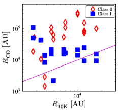
Figure 5: $R_{\rm CO}$ is plotted against $R_{\rm 10K}$, the radius of the modeled envelope within 10 K radius. The black line is for $R_{\rm CO}$ = $R_{\rm 10K}$, showing that almost all sources follow $R_{\rm CO}$ $>$ $R_{\rm 10K}$ and that $R_{\rm CO}$ is larger for Class 0 than Class I sources.

Table 2: Outflow properties of the red and blue outflow lobes of Class 0 sources.

Source	Trans.	Inclination	Lobe	$R_{\rm CO}$	$t_{\rm{dyn}}$	$M_{\rm outflow}$	$\dot{M}$	$F_{\rm CO}$	$L_{\rm{kin}}$
		[$\degr$]		[AU]	[103 yr]	[M⊙]	[M⊙ yr-1]	[M⊙ yr-1km s-1]	[L⊙]
L1448MM	CO 3–2	50	Blue	5.9$\times$104	5.5	9.0$\times$10-2	7.2$\times$10-5	2.0$\times$10-3	2.8$\times$100
			Red	5.9$\times$104	9.7	6.2$\times$10-2	2.8$\times$10-5	1.7$\times$10-3	2.3$\times$100
NGC1333-IRAS~2A	CO 6–5	70	Blue	1.4$\times$104	2.9	7.9$\times$10-3	2.0$\times$10-5	3.4$\times$10-4	1.7$\times$10-1
			Red	1.4$\times$104	3.9	2.2$\times$10-2	4.0$\times$10-5	2.0$\times$10-3	1.7$\times$100
	CO 3–2	70	Blue	2.4$\times$104	4.8	8.5$\times$10-2	1.3$\times$10-4	2.6$\times$10-3	1.2$\times$100
			Red	2.4$\times$104	6.4	6.9$\times$10-2	7.7$\times$10-5	4.8$\times$10-3	5.4$\times$100
NGC1333-IRAS~4A	CO 6–5	50	Blue	2.5$\times$104	5.3	8.1$\times$10-3	6.7$\times$10-6	1.5$\times$10-4	5.6$\times$10-2
			Red	3.5$\times$104	8.4	1.9$\times$10-2	9.9$\times$10-6	5.4$\times$10-4	5.4$\times$10-1
	CO 3–2	50	Blue	2.8$\times$104	6.1	2.1$\times$10-2	1.5$\times$10-5	3.5$\times$10-4	1.6$\times$10-1
			Red	3.9$\times$104	9.3	2.5$\times$10-2	1.2$\times$10-5	1.7$\times$10-3	1.8$\times$100
NGC1333-IRAS~4B	CO 6–5	10	Blue	2.4$\times$103	0.6	8.2$\times$10-4	1.6$\times$10-6	3.2$\times$10-5	7.4$\times$10-3
			Red	1.2$\times$103	0.4	7.3$\times$10-4	2.2$\times$10-6	1.6$\times$10-4	1.8$\times$10-1
	CO 3–2	10	Blue	3.5$\times$103	0.8	8.3$\times$10-4	1.3$\times$10-6	2.9$\times$10-5	1.1$\times$10-2
			Red	2.4$\times$103	0.9	2.7$\times$10-3	3.6$\times$10-6	1.9$\times$10-4	1.8$\times$10-1
L1527	CO 6–5	70	Blue	1.5$\times$104	9.1	2.3$\times$10-3	1.8$\times$10-6	3.1$\times$10-5	9.9$\times$10-3
			Red	1.1$\times$104	6.5	2.5$\times$10-3	2.7$\times$10-6	1.1$\times$10-4	7.5$\times$10-2
	CO 3–2	70	Blue	3.2$\times$104	20.6	1.0$\times$10-2	3.5$\times$10-6	6.1$\times$10-5	2.0$\times$10-2
			Red	1.1$\times$104	6.5	9.0$\times$10-3	9.8$\times$10-6	3.8$\times$10-4	2.6$\times$10-1
Ced110-IRS4	CO 6–5	30	Blue	3.8$\times$103	4.2	2.7$\times$10-4	1.8$\times$10-7	2.1$\times$10-6	4.6$\times$10-4
			Red	3.8$\times$103	4.7	2.5$\times$10-4	1.5$\times$10-7	4.1$\times$10-6	2.0$\times$10-3
BHR71	CO 6–5	70	Blue	4.4$\times$104	13.4	3.4$\times$10-2	1.8$\times$10-5	7.7$\times$10-4	6.2$\times$10-1
			Red	4.0$\times$104	8.5	6.9$\times$10-2	5.8$\times$10-5	7.7$\times$10-4	3.3$\times$10-1
IRAS~15398	CO 6–5	30	Blue	2.6$\times$103	1.4	3.4$\times$10-4	1.7$\times$10-6	6.4$\times$10-6	1.4$\times$10-3
			Red	2.6$\times$103	1.2	2.7$\times$10-4	1.5$\times$10-6	2.6$\times$10-5	2.0$\times$10-2
	CO 3–2	30	Blue	3.2$\times$103	1.8	4.4$\times$10-4	1.8$\times$10-6	9.2$\times$10-6	2.5$\times$10-3
			Red	2.0$\times$103	0.9	2.5$\times$10-4	1.9$\times$10-6	2.8$\times$10-5	2.0$\times$10-2
L483MM	CO 6–5	70	Blue	1.2$\times$104	5.2	4.2$\times$10-3	5.7$\times$10-6	6.7$\times$10-5	1.6$\times$10-2
			Red	1.0$\times$104	4.4	3.4$\times$10-3	5.4$\times$10-6	2.1$\times$10-4	1.5$\times$10-1
	CO 3–2	70	Blue	1.4$\times$104	6.2	7.0$\times$10-3	8.0$\times$10-6	7.7$\times$10-5	1.6$\times$10-2
			Red	1.0$\times$104	4.4	8.5$\times$10-3	1.4$\times$10-5	5.1$\times$10-4	3.4$\times$10-1
Ser-SMM1	CO 6–5	50	Blue	3.4$\times$104	8.4	1.6$\times$10-2	8.2$\times$10-6	1.5$\times$10-4	5.7$\times$10-2
			Red	1.8$\times$104	3.9	1.2$\times$10-2	1.4$\times$10-5	8.7$\times$10-4	9.8$\times$10-1
	CO 3–2	50	Blue	3.4$\times$104	8.6	6.4$\times$10-2	3.3$\times$10-5	6.7$\times$10-4	2.8$\times$10-1
			Red	1.8$\times$104	3.9	3.3$\times$10-2	3.7$\times$10-5	2.3$\times$10-3	2.7$\times$100
Ser-SMM4	CO 6–5	30	Blue	1.8$\times$104	4.6	2.4$\times$10-2	1.5$\times$10-5	2.5$\times$10-4	9.3$\times$10-2
			Red	1.8$\times$104	7.3	2.8$\times$10-2	1.1$\times$10-5	5.9$\times$10-4	5.8$\times$10-1
	CO 3–2	30	Blue	1.8$\times$104	4.6	1.6$\times$10-1	9.9$\times$10-5	2.0$\times$10-3	8.3$\times$10-1
			Red	1.8$\times$104	7.6	1.3$\times$10-1	4.7$\times$10-5	2.8$\times$10-3	2.9$\times$100
Ser-SMM3	CO 6–5	50	Blue	4.6$\times$103	1.0	6.9$\times$10-3	3.1$\times$10-5	6.0$\times$10-4	2.6$\times$10-1
			Red	4.6$\times$103	1.6	3.0$\times$10-3	8.1$\times$10-6	4.9$\times$10-4	5.4$\times$10-1
	CO 3–2	50	Blue	4.6$\times$103	1.0	2.7$\times$10-2	1.2$\times$10-4	2.4$\times$10-3	1.0$\times$100
			Red	4.6$\times$103	1.6	1.1$\times$10-2	3.0$\times$10-5	1.8$\times$10-3	1.9$\times$100
B335	CO 6–5	70	Blue	6.2$\times$103	3.4	4.7$\times$10-4	9.9$\times$10-7	2.3$\times$10-5	9.4$\times$10-3
			Red	8.8$\times$103	4.8	1.3$\times$10-3	1.9$\times$10-6	9.0$\times$10-5	7.6$\times$10-2
	CO 3–2	70	Blue	1.0$\times$104	5.3	3.7$\times$10-3	4.9$\times$10-6	1.3$\times$10-4	6.2$\times$10-2
			Red	7.5$\times$103	4.1	5.4$\times$10-3	9.3$\times$10-6	4.7$\times$10-4	4.3$\times$10-1
L723MM	CO 6–5	50	Blue	1.2$\times$104	4.1	6.0$\times$10-3	6.6$\times$10-6	1.8$\times$10-4	1.0$\times$10-1
			Red	1.2$\times$104	3.8	7.5$\times$10-3	8.5$\times$10-6	5.5$\times$10-4	6.3$\times$10-1
	CO 3–2	50	Blue	1.8$\times$104	6.0	3.0$\times$10-2	2.2$\times$10-5	6.5$\times$10-4	3.7$\times$10-1
			Red	1.8$\times$104	5.8	4.2$\times$10-2	3.2$\times$10-5	2.2$\times$10-3	2.8$\times$100
L1157	CO 3–2	70	Blue	4.4$\times$104	16.8	1.2$\times$10-1	4.9$\times$10-5	5.0$\times$10-4	1.9$\times$10-1
			Red	5.2$\times$104	14.1	1.5$\times$10-1	7.3$\times$10-5	3.2$\times$10-3	3.1$\times$100

Table 3: Outflow properties of the red and blue outflow lobes of Class I sources.

Source	Trans.	Inclination	Lobe	$R_{\rm CO}$	$t_{\rm{dyn}}$	$M_{\rm outflow}$	$\dot{M}$	$F_{\rm CO}$	$L_{\rm{kin}}$
		[$\degr$]		[AU]	[103 yr]	[M⊙]	[M⊙ yr-1]	[M⊙ yr-1km s-1]	[L⊙]
L1489	CO 6–5	50	Blue	3.5$\times$103	1.2	4.0$\times$10-5	1.5$\times$10-7	1.8$\times$10-6	3.2$\times$10-4
			Red	2.1$\times$103	1.3	1.3$\times$10-4	4.6$\times$10-7	2.3$\times$10-5	2.0$\times$10-2
	CO 3–2	50	Blue	3.5$\times$103	1.2	6.9$\times$10-4	2.5$\times$10-6	3.9$\times$10-5	1.3$\times$10-2
			Red	2.1$\times$103	1.3	7.1$\times$10-4	2.5$\times$10-6	1.2$\times$10-4	1.1$\times$10-1
L1551-IRS5	CO 3–2	70	Blue	1.7$\times$104	8.2	7.4$\times$10-3	6.4$\times$10-6	9.3$\times$10-5	2.7$\times$10-2
			Red	1.7$\times$104	6.7	9.6$\times$10-3	1.0$\times$10-5	4.2$\times$10-4	3.1$\times$10-1
TMR1	CO 6–5	50	Blue	4.9$\times$103	2.9	1.2$\times$10-4	1.8$\times$10-7	2.0$\times$10-6	4.9$\times$10-4
			Red	3.5$\times$103	4.5	2.4$\times$10-4	2.3$\times$10-7	8.0$\times$10-6	4.8$\times$10-3
	CO 3–2	50	Blue	4.9$\times$103	3.0	2.6$\times$10-4	3.8$\times$10-7	5.1$\times$10-6	1.4$\times$10-3
			Red	3.5$\times$103	4.5	5.8$\times$10-4	5.7$\times$10-7	2.0$\times$10-5	1.3$\times$10-2
TMC1A	CO 6–5	50	Blue	5.6$\times$103	1.4	2.3$\times$10-4	7.2$\times$10-7	1.3$\times$10-5	7.6$\times$10-3
			Red	2.1$\times$103	1.8	4.0$\times$10-6	9.5$\times$10-9	3.7$\times$10-7	2.4$\times$10-4
	CO 3–2	50	Blue	5.6$\times$103	1.6	2.8$\times$10-3	7.8$\times$10-6	1.1$\times$10-4	3.7$\times$10-2
			Red	1.7$\times$103	1.5	1.4$\times$10-4	4.1$\times$10-7	1.8$\times$10-5	1.4$\times$10-2
TMC1	CO 6–5	50	Blue	3.5$\times$103	1.2	1.3$\times$10-4	4.7$\times$10-7	3.2$\times$10-6	4.0$\times$10-4
			Red	4.9$\times$103	1.6	3.8$\times$10-4	1.1$\times$10-6	5.0$\times$10-5	4.4$\times$10-2
	CO 3–2	50	Blue	3.5$\times$103	1.2	5.6$\times$10-4	2.0$\times$10-6	2.7$\times$10-5	7.9$\times$10-3
			Red	2.1$\times$103	0.7	1.4$\times$10-3	8.9$\times$10-6	4.2$\times$10-4	3.7$\times$10-1
HH46-IRS	CO 6–5	50	Blue	1.1$\times$104	9.9	2.6$\times$10-3	1.2$\times$10-6	1.2$\times$10-5	2.9$\times$10-3
			Red	2.5$\times$104	7.9	3.2$\times$10-2	1.8$\times$10-5	7.7$\times$10-4	6.5$\times$10-1
	CO 3–2	50	Blue	1.6$\times$104	13.6	2.2$\times$10-2	7.2$\times$10-6	2.5$\times$10-4	1.7$\times$10-1
			Red	2.5$\times$104	7.9	2.2$\times$10-2	1.2$\times$10-5	8.1$\times$10-4	9.3$\times$10-1
DK~Cha	CO 6–5	10	Blue	1.8$\times$103	1.6	1.8$\times$10-4	1.3$\times$10-7	6.6$\times$10-7	7.3$\times$10-5
			Red	1.8$\times$103	0.9	1.1$\times$10-4	1.4$\times$10-7	2.5$\times$10-6	4.4$\times$10-4
GSS30-IRS1	CO 6–5	30	Blue	1.5$\times$104	5.5	1.5$\times$10-2	7.9$\times$10-6	5.1$\times$10-5	1.1$\times$10-2
			Red	1.5$\times$104	4.9	8.9$\times$10-3	5.1$\times$10-6	2.0$\times$10-4	1.6$\times$10-1
	CO 3–2	30	Blue	1.5$\times$104	5.5	2.1$\times$10-2	1.1$\times$10-5	6.0$\times$10-5	8.8$\times$10-3
			Red	1.5$\times$104	4.9	2.4$\times$10-2	1.4$\times$10-5	4.6$\times$10-4	3.0$\times$10-1
Elias~29	CO 6–5	30	Blue	7.5$\times$103	3.1	6.4$\times$10-4	5.7$\times$10-7	4.4$\times$10-6	1.2$\times$10-3
			Red	5.0$\times$103	1.7	6.3$\times$10-4	1.0$\times$10-6	3.9$\times$10-5	2.7$\times$10-2
	CO 3–2	30	Blue	7.5$\times$103	3.6	1.4$\times$10-3	1.1$\times$10-6	6.6$\times$10-6	1.0$\times$10-3
			Red	7.5$\times$103	3.3	1.8$\times$10-3	1.5$\times$10-6	5.7$\times$10-5	3.9$\times$10-2
Oph-IRS63	CO 6–5	50	Blue	3.8$\times$103	1.6	1.0$\times$10-4	2.8$\times$10-7	4.3$\times$10-6	2.1$\times$10-3
			Red	3.8$\times$103	4.2	8.6$\times$10-5	9.0$\times$10-8	2.1$\times$10-6	8.3$\times$10-4
	CO 3–2	50	Blue	8.8$\times$103	3.7	7.0$\times$10-4	8.4$\times$10-7	5.6$\times$10-6	1.5$\times$10-3
			Red	5.0$\times$103	7.4	5.0$\times$10-4	3.0$\times$10-7	5.2$\times$10-6	2.2$\times$10-3
RNO91	CO 6–5	50	Blue	3.1$\times$103	1.0	2.5$\times$10-4	1.1$\times$10-6	2.9$\times$10-5	2.1$\times$10-2
			Red	1.9$\times$103	2.5	7.3$\times$10-5	1.3$\times$10-7	1.1$\times$10-6	1.8$\times$10-4
	CO 3–2	50	Blue	6.2$\times$103	2.0	3.5$\times$10-3	7.7$\times$10-6	1.0$\times$10-4	4.1$\times$10-2
			Red	1.9$\times$103	2.5	2.3$\times$10-4	4.0$\times$10-7	2.3$\times$10-6	2.6$\times$10-4

3.2 Outflow parameters

In the following, different outflow parameters, including mass, force and luminosity, are measured. These parameters have previously been determined from lower-$J$ lines for several young stellar objects (e.g., Cabrit & Bertout 1992; Bontemps et al. 1996; Hogerheijde et al. 1998; Hatchell et al. 2007; Curtis et al. 2010; van der Marel et al. 2013; Dunham et al. 2014) and more recently from CO 6–5 by van Kempen et al. (2009b) and Yıldız et al. (2012) for a small subset of the sources presented here. All results are listed in Tables 8 and 9. Uncertainties in the methods are discussed extensively in van der Marel et al. (2013).

3.2.1 Outflow mass

One of the most basic outflow parameters is the mass. The inferred mass depends on three assumptions: the line opacity, the distribution of level populations, and the CO abundance with respect to H₂. In the following, we assume that the line wings are optically thin, as has been demonstrated observationally for CO 6–5 for a few sources with massive outflows (e.g., NGC 1333-IRAS 4A, Yıldız et al. 2012). CO 3–2 emission is also assumed optically thin in the following, although that assumption may not be fully valid (see discussion below). The level populations are assumed to follow a Boltzmann distribution with a single temperature, $T_{\rm ex}$. Finally, the abundance ratio is taken as [H₂/¹²CO]=1.2$\times$10⁴, as in Yıldız et al. (2012).

The upper level column density per statistical weight in a single pixel (4$\aas@@fstack{\prime\prime}$5$\times$4$\aas@@fstack{\prime\prime}$5 for CO 6–5, 7$\aas@@fstack{\prime\prime}$5$\times$7$\aas@@fstack{\prime\prime}$5 for CO 3–2) is calculated as

$$\frac{N_{\rm u}}{g_{\rm u}}=\frac{\beta\nu^{2}\int T_{\rm mb}{\rm d}V}{A_{\rm ul}\,g_{\rm u}}\ .$$ (1)

The constant $\beta$ is $8\pi k/hc^{3}$=1937 cm^-2 (GHz² K km)^-1. The remaining parameters are for the specific transition, where $\nu$ is the frequency, $A_{\rm ul}$ is the Einstein $A$ coefficient and $g_{\rm u}$=2$J$+1.

The total CO column density in a pixel, $N_{\rm total}$, is

$$N_{\rm total}=\frac{N_{\rm u}}{g_{\rm u}}Q(T)e^{E_{\rm u}/kT_{\rm ex}}\ ;$$ (2)

$Q(T)$ is the partition function corresponding to a specific excitation temperature, $T_{\rm ex}$, which is assumed to be 75 K for both CO 3–2 and CO 6–5 observations (van Kempen et al. 2009b; Yıldız et al. 2012, 2013). Changing $T_{\rm ex}$ by $\pm 30$ K changes the inferred column densities by only 10–20%.

The mass is calculated as

$$M_{\rm outflow}=\mu_{\rm H_{2}}\,m_{\rm H}\,A\,\left[\frac{\rm H_{2}}{{}^{12}{\rm CO}}\right]\sum_{j}N_{{\rm total},j}$$ (3)

where the factor $\mu_{\mathrm{H_{2}}}$=2.8 includes the contribution of helium (Kauffmann et al. 2008) and $m_{\rm H}$ is the mass of the hydrogen atom. $A$ is the surface area of one pixel $j$. The sum is over all outflow pixels.

The mass may be underestimated if the ¹²CO line emission is optically thick. ¹³CO data exist toward most outflows (see above) but the $S/N$ of these data is typically too low to properly measure the opacity in the line wings, except for at the source position where the signal naturally is the strongest. The ¹³CO line wings do not extend beyond the inner velocity limits. NGC1333-IRAS 4A is one of the few sources where line wings are detected in ¹³CO at the outflow positions (Fig. 11 in Yıldız et al. 2012), and it is clear that at the velocity ranges considered here, the line emission is optically thin ($\tau<1$); the same is true for the outflows studied by van der Marel et al. (2013) in CO 3–2 emission in Ophiuchus (their Fig. 4), where deep pointed observations of ¹³CO 3–2 were required to measure the opacity. That study concluded that the opacity does not play a significant role when determining the outflow parameters. Similarly, Dunham et al. (2014) conclude that CO 3–2 may be optically thick at velocities less than 2 km s^-1 offset from the source velocity, velocities which are excluded from our analysis because of the risk of cloud contamination. Potentially more problematic is the missing mass at low velocities. The missing mass is moving close to the systemic velocity and it is not possible to disentangle this mass from the surrounding cloud material, an effect which may introduce a typical uncertainty of a factor of 2–3 (Downes & Cabrit 2007). However, the correction factors derived by the same authors and implemented here account for that missing mass. ¹²CO 6–5 emission will be less affected by this confusion than the ¹²CO 3–2 emission, simply because of the different excitation conditions required.

3.2.2 Outflow force

One of the most important outflow parameters is the outflow force, $F_{\rm CO}$. The best method for computing the outflow force is still debated and the results suffer from ill-constrained observational parameters, such as inclination, $i$. van der Marel et al. (2013) compare seven different methods proposed in the literature to calculate outflow forces. The “separation method” (see below) in their paper is found to be the preferred method, which is less affected by the observational biases. The method can also be applied to low spatial resolution observations or incomplete maps. Uncertainties are estimated to be a factor of 2–3.

In the following, the outflow force is calculated separately for the blue– and red–shifted lobes, only including emission above the 3$\sigma$ level. The mass is calculated for each channel separately and multiplied by the central velocity of that particular channel. The integral runs over velocities from $V_{\rm in}$ to $V_{\rm out}$. They are then summed and the sum is over all pixels $j$ in the map with outflow emission. The outflow force is calculated for the red- and blue-shifted outflow lobes separately. This method is formulated as:

$$F_{\rm CO}=c_{i}\frac{V_{\rm max}\sum_{j}\left[\int M(V^{\prime})V^{\prime}{\rm d}V^{\prime}\right]_{j}}{R_{\rm CO}},$$ (4)

where $c_{i}$ is the inclination correction (Table 7), and $R_{\rm CO}$ is the projected size of the red- or blue-shifted outflow lobe. The outflow force is computed separately from the CO 3–2 and 6–5 maps of the same source (see Tables 8 and 9).

The difference in outflow force between the red and blue outflow lobes ranges from $\sim$1 up to a factor of 10. For sources with a low outflow force such as Oph IRS63 ($<$10^-5 M_⊙ yr^-1 km s^-1) this is a result of differences in the inferred outflow mass per lobe, which, in these specific cases, is primarily a result of low $S/N$. In these cases, the overall uncertainty on the outflow force is high, up to a factor of 10. In other cases, such as HH 46 as mentioned above, there is a real asymmetry between the different lobes which is caused by a difference in the surrounding environment. In the following, only the sum of the outflow forces of both lobes as measured from each outflow lobe will be used.

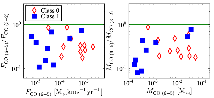
Figure 6: Outflow forces (left) and outflow masses (right), calculated from CO 6–5 and 3–2 emission are compared for Class 0 and I sources. Green lines are for a ratio of 1.

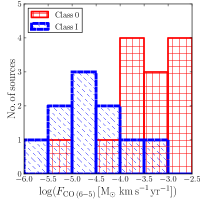
Figure 7: Histograms of calculated total outflow force $F_{\rm CO}$ are shown for Class 0 (red) and Class I (blue) sources.

Figure 6 shows how the outflow forces and outflow masses calculated from CO 3–2 and 6–5 differ. For strong outflows, there is a factor of a few difference in the two calculations, with differences up to an order of magnitude for the weaker outflow sources. Although the CO 6–5 emission suffers less from opacity effects and so recovers more emission / mass at lower velocities, this effect is overwhelmed by the lower $S/N$ of the CO 6–5 emission. The fact that the masses and outflow forces derived from the 6–5 data are systematically lower than those from the 3–2 data is likely due to the same effect (van der Marel et al. 2013). Moreover, if CO 6–5 traces slightly warmer gas than CO 3–2 (Yıldız et al. 2013) then the mass traced by this line will be lower than that traced by CO 3–2. Both effects work to systematically lower the CO 6–5 masses, which in turn leads to lower outflow forces.

Figure 7 displays $F_{\rm CO}$ from CO 6–5 for Class 0 and Class I sources separately. Generally, Class 0 sources have higher outflow forces and are thus more powerful than their Class I counterparts (Bontemps et al. 1996). The Class I source with an exceptionally high outflow force is HH46.

3.3 Other outflow parameters

Other outflow parameters that characterize the outflow activity are the dynamical age, $t_{\rm dyn}$, mass outflow rate, $\dot{M}_{\rm outflow}$, and kinetic luminosity, $L_{\rm kin}$.

Assuming that the outflow moves with a constant velocity over the extent of the outflow, the dynamical age is determined as

$$t_{\rm dyn}=\frac{R_{\rm CO}}{V_{\rm max}}\ .$$ (5)

This age is a lower limit on the age of the protostar (Curtis et al. 2010) if the outflowing material is decelerated, e.g., through interactions with the ambient surrounding material. On the other hand, the outflow may be significantly younger since the velocities of the central jet that drives the molecular outflow are typically higher than 100 km s^-1 and what is observed in these colder low-$J$ CO lines may just be the outer shell which is currently undergoing acceleration, not deceleration. See, e.g., Downes & Cabrit (2007) for a more complete discussion. The outflow mass loss rate is computed according to

$$\dot{M}_{\rm outflow}=\frac{M_{\rm outflow}}{t_{\rm dyn}}\ .$$ (6)

The kinetic luminosity is given by

$$L_{\rm kin}=\frac{1}{2}F_{\rm CO}V_{\rm max}\ .$$ (7)

Outflow parameters of $F_{\rm CO}$, $\dot{M}$, and $L_{\rm kin}$ with inclination corrections are presented in Tables 8 and 9. However, $M_{\rm outflow}$, $R_{\rm CO}$, $t_{\rm dyn}$, and $V_{\rm max}$ are not corrected for inclination, since they are measured quantities. The median values of the results are given in Table 4.

Table 4: Median values of the outflow parameters.

	$M_{\rm outflow}$	$\dot{M}$	$F_{\rm CO}$	$L_{\rm{kin}}$
	[$M_{\odot}$]	[$M_{\odot}$ yr-1]	[$M_{\odot}$ kms yr-1]	[$L_{\odot}$]
CO 6–5
Class 0	9.8$\times$10-3	1.5$\times$10-5	6.9$\times$10-4	6.0$\times$10-1
Class I	3.4$\times$10-4	8.4$\times$10-6	2.8$\times$10-5	1.2$\times$10-1
Total	2.2$\times$10-3	1.0$\times$10-5	1.4$\times$10-4	1.9$\times$10-1
CO 3–2
Class 0	7.2$\times$10-2	5.4$\times$10-5	2.9$\times$10-3	2.9$\times$100
Class I	3.1$\times$10-3	3.0$\times$10-5	1.4$\times$10-4	1.4$\times$100
Total	1.7$\times$10-2	3.3$\times$10-5	5.2$\times$10-4	1.9$\times$100

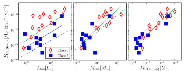
Figure 8: Correlations of $F_{\rm CO}$ with $L_{\rm bol}$, $M_{\rm env}$, and $M_{\rm outflow}$, where $F_{\rm CO}$ is determined from the CO 6–5 data. Red and blue symbols indicate Class 0 and Class I sources, respectively. The green solid line is the fit to all values and the blue solid line is the fit to the Class I sources alone. Blue and green dashed lines are the best fits from Bontemps et al. (1996).

3.4 Correlations

Most previous studies of the outflow force were done using CO 1–0, 2–1, or 3–2 (e.g., Cabrit & Bertout 1992; Bontemps et al. 1996; Hogerheijde et al. 1998; Hatchell et al. 2007; van Kempen et al. 2009c; Dunham et al. 2014). The opacity decreases with excitation, as suggested by, e.g., the observations reported in Dunham et al. (2014), but without targeted, deep surveys of ¹³CO, it is difficult to quantify how much the CO column density is underestimated. Furthermore, cloud or envelope emission may contribute to the emission at the lowest outflow velocities at which the bulk of the mass is flowing. With our CO 6–5 observations, some of the above-mentioned issues can be avoided, or their effects can be lessened. Thus, it is important to revisit the correlations of outflow force with bolometric luminosity and envelope mass using these new measurements.

In Fig. 8, $F_{\rm CO}$ is plotted against $L_{\rm bol}$, $M_{\rm env}$, and $M_{\rm outflow}$, where the $F_{\rm CO}$ and $M_{\rm outflow}$ values are taken from the CO 6–5 data. The best fit between $F_{\rm CO}$ and $L_{\rm bol}$ is shown with the green line corresponding to

$${\rm log}(F_{\rm CO})=-(4.71\pm 0.02)+(1.13\pm 0.37)\,{\rm log}(L_{\rm bol})\ .$$ (8)

Outflows from Class 0 and Class I sources are well-separated; Class 0 sources show more powerful outflows compared to Class I sources of similar luminosity. The Pearson correlation coefficients are $r$=0.62, 0.83, and 0.64 for all sources, Class 0, and Class I sources, corresponding to confidences of 2.9, 2.9, and 1.9$\sigma$, respectively.

The best fit between $F_{\rm CO}$ and $M_{\rm env}$ is described as

$${\rm log}(F_{\rm CO})=-(3.95\pm 0.37)+(1.24\pm 0.21)\,{\rm log}(M_{\rm env})$$ (9)

and Pearson correlation coefficients are $r$=0.81, 0.82, and 0.56 (3.8, 2.8 and 1.7$\sigma$) for all sources, Class 0, and Class I, respectively. Since early Class 0 sources have higher accretion rates their outflow force is much higher than for the Class I sources (see, e.g., Bontemps et al. 1996, for a full discussion). Finally, as expected, a strong correlation is found between $F_{\rm CO}$ and $M_{\rm outflow}$ with a Pearson correlation coefficient of $r$=0.92 for all sources (4.3$\sigma$), not surprisingly since $F_{\rm CO}$ is nearly proportional to $M_{\rm outflow}$. The best fit is described as

$${\rm log}(F_{\rm CO})=-(1.71\pm 0.02)+(0.88\pm 0.62)\,{\rm log}(M_{\rm CO})\ .$$ (10)

Previously, Bontemps et al. (1996) surveyed 45 sources using CO 2–1 observations with small-scale maps. In Fig. 8, the blue and green dashed lines of $F_{\rm CO}$ vs. $L_{\rm bol}$ and $M_{\rm env}$ show the fit results from their Figs. 5 and 6 (Bontemps et al. 1996). Since their number of Class I sources is higher than Class 0 sources, the fit was only done for Class I sources in $F_{\rm CO}$ vs. $L_{\rm bol}$. In Fig. 8, the blue solid line only shows the fit for Class I sources and the correlation is described by,

$${\rm log}(F_{\rm CO})=-(5.14\pm 0.29)+(0.98\pm 0.55)\,{\rm log}(L_{\rm bol})\ .$$ (11)

In the $F_{\rm CO}$ vs. $M_{\rm env}$ plot, the fits are shown as green lines for the entire sample. The Bontemps et al. (1996) sample is weighted toward lower luminosities ($<10$ L_bol), where our $F_{\rm CO}$ measurements from the CO 6–5 data follow their relation for Class I sources obtained from 2–1 data, but with a shift to a factor of a few higher values of $F_{\rm CO}$. However, given the scatter in the results for low $L_{\rm bol}$ sources, this difference is hardly significant.

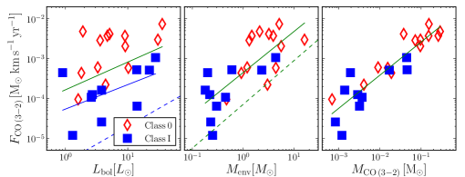
Figure 19: Correlations between $F_{\rm CO}$ as measured from CO 3–2 and bolometric luminosity, envelope mass and outflow mass as determined from CO 3–2.

Examining the same outflow parameters measured using the CO 3–2 transition, and their correlation with the same outflow parameters, a similar picture arises (Fig. 19). However, for the sources in our sample, the correlations follow the same trend but they are somewhat weaker. In particular, the correlation with $L_{\rm bol}$ is at the $\sim$2.7$\sigma$ level, whereas the correlation with $M_{\rm env}$ is 3.1$\sigma$. Although the measured values of, e.g., $F_{\rm CO}$, fill out the same parameter space as when the measurements are done with CO 6–5, the scatter is larger. The scatter remains on the order of one order of magnitude, which is similar to the scatter reported in the literature (e.g., Bontemps et al. 1996), but because of the limited source sample (20 sources with $F_{\rm CO}$ measurements) it is difficult to compare these 3–2 measurements with what is presented in the literature.

3.5 Radiative feedback from UV heating

The quiescent gas is traced by the narrow (FWHM $\lesssim$1 km s^-1) ¹³CO 6–5 emission, which has been mapped over a 1^′ region around the source position. As the contour maps in Figs. 17 and 18 show, the emission is strongly centrally concentrated and does not extend beyond the mapped region except for special cases like NGC 1333 IRAS 4A (Yıldız et al. 2012). The observed emisison has two contributions: (i) the dense envelope heated ‘passively’ by the luminosity of the protostar, i.e., the dust in the envelope absorbs all the protostellar luminosity and is heated by it, and this temperature is then transferred to the gas through gas-dust collisions; (ii) the gas heated by UV photons created by protostellar accretion or by shocks in the outflow, and escaping from the immediate protostellar surroundings, for example through outflow cavities, to larger distances. Here the temperature of the gas is higher than that of the dust.

The first component has been modeled by Kristensen et al. (2012) for all our sources and dust temperatures in excess of 10 K are typically found out to between 2.5$\times$10³ up to 1.5$\times$10⁴ AU from the sources. There is evidence that the dust may be further heated on large scales by the UV photons generated by the accreting protostar (Hatchell et al. 2013; Sicilia-Aguilar et al. 2013). We here quantify the second component, which is the gas with temperatures higher than that of the dust, in excess of the passively heated envelope. This second mechanism operates on larger scales and is most relevant to preventing further collapse or fragmentation of the core (Offner et al. 2009, 2010).

To isolate this second component, the method outlined in Yıldız et al. (2012) is used. The ¹³CO 6–5 envelope emission (component (i)) is modeled using the temperature and density profiles from Kristensen et al. (2012) together with the C¹⁸O constant abundance results provided in Yıldız et al. (2013, Table 5). For the three NGC 1333 sources, drop abundance profiles are used in which CO is frozen out in some part of the envelope; for NGC 1333-IRAS 2A the results from Yıldız et al. (2010) are taken, whereas for NGC 1333-IRAS 4A and NGC 1333-IRAS 4B the models from Yıldız et al. (2012) are adopted. These C¹⁸O abundances are then multiplied by the [¹³C]/[¹⁸O] abundance ratio of 8.5 (Langer & Penzias 1990) and the ¹³CO emission is computed using the non-LTE excitation line radiative transfer code RATRAN (Hogerheijde & van der Tak 2000). The turbulent width for all the model ¹³CO spectra is taken as 0.9 km s^-1, except for NGC 1333-IRAS 4A and NGC 1333-IRAS 4B where the values from Yıldız et al. (2012) are used. The resulting emission map is convolved with the relevant observing beam.

Figures 20-25 present 7$\times$7 pixel maps ($\sim$30″ $\times$ 30″; 1 pixel = 4.5″) around the central position of each source in the ¹²CO and ¹³CO 6–5 transitions. The modeled envelope emission (component (i)) is shown as red lines overplotted on the ¹³CO maps. The right-most panels present the difference between the model envelope emission and the observed emission, which is the UV-heated gas. Two illustrative maps are shown for B335 and L483mm in Fig. 9.

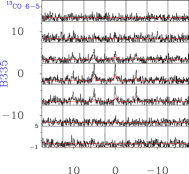
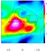
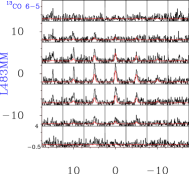
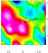
Figure 9: ¹³CO spectral maps in black overlaid with the model envelope spectra in red shown on the left panels. On the right panels, color maps of the UV heated gas distribution are shown. These are obtained by subtracting the model envelope emission from the observed spectra on a pixel-by-pixel basis. The sources are B335 (top) and L483mm (bottom). The axes show the offsets ($\Delta$$\alpha$, $\Delta$$\delta$) in arcsec. The color scale is in units of K km s^-1.

Most sources show some excess ¹³CO emission on scales of 5″–10″ or 1000–2000 AU at the average distance of 200 pc. The only exceptions are L1527 and Oph IRS63. The emission is almost always aligned with one (12/24 sources) or both (4/24 sources) outflow lobes. A few sources show widely distributed ¹³CO emission (6/24 sources). More Class 0 sources show excess emission along the direction of the outflow (11/13 sources) than Class I’s do (5/11) but this may be a $S/N$ effect.

The typical ¹³CO 6–5 line width is $\lesssim$1 km s^-1, and so the emission is not part of the swept-up outflow gas as illustrated in more detail for the case of NGC 1333-IRAS 4A by Yıldız et al. (2012). The only known mechanism to create this excess narrow emission is by UV photons generated from the protostellar accretion process and subsequently escaping through the outflow cavities (Spaans et al. 1995).

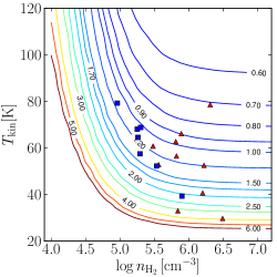
Figure 26: ¹³CO 3–2/6–5 intensity ratio as a function of density and gas temperature calculated via RADEX for $N(^{13}{\rm CO})$=1.5$\times$10¹⁴ cm^-2. Red markers indicate the observed intensity ratios for the central pixels for Class 0 sources whereas blue markers are for Class I sources. Both pixels are taken to be 15$\arcsec$ diameter. The corresponding densities are the values at the 7.5$\arcsec$ radius found in the power-law envelope models of Kristensen et al. (2012).

To estimate the effects of the UV radiation on these scales, it is first important to estimate the temperature of the gas compared with that of the dust. Figure 26 shows model ¹³CO 3–2/6–5 line ratios for a grid of kinetic temperatures and densities, with the observed values for each source overplotted at the $7.5^{\prime\prime}$ radius density. The inferred temperatures are in the range of 30–80 K, consistent with the model predictions from Visser et al. (2012) on spatial scales of a few 1000 AU. For comparison, the typical dust envelope temperature at this distance is $\sim$15–25 K and thus the gas is heated to higher temperatures by more than a factor of 2.

The mass of the UV-heated gas (component (ii)) is calculated on the basis of the residual after subtracting the ¹³CO model envelope emission (component (i)) from the observed ¹³CO emission. The mass is then calculated via the residual emission by assuming $T_{\rm ex}$=50 K and CO/H₂=1.2$\times$10^-4, where the value of $T_{\rm ex}$ is chosen because it is the median value for ¹³CO as reported in Yıldız et al. (2013) based on transitions from 2–1 up to 10–9. In order to compare UV-heated gas mass to the total outflow gas mass, the outflow mass is recalculated from ¹²CO 6–5 over the same ($\sim$30″ $\times$ 30″) area, using $T_{\rm ex}$=75 K to be consistent with all other ¹²CO mass calculations. In Table 10, the masses calculated for the envelope, UV-heated gas and outflow gas are tabulated.

The mass of the UV-heated gas is typically a factor of 10 to 100 times lower than the total envelope mass (Fig. 10a) and a factor of just a few up to 50 compared to the envelope mass within the 30$\arcsec$$\times$30$\arcsec$ region. There is no correlation with evolution; i.e., the fraction of UV-heated gas compared to the total envelope mass does not change from Class 0 to Class I. Similarly there is no correlation between the mass of the UV-heated gas and the density at 1000 AU (Fig. 10b), which may suggest that the emission is independent of density and thus the emission is thermalized.

Compared with the outflow masses, the UV-heated gas masses (component (ii)) are typically a few times higher, as also found for NGC 1333-IRAS 4A in Yıldız et al. (2012). They follow a remarkably tight correlation with a Pearson correlation coefficient of 0.86 (3.1$\sigma$; Fig. 10c). Furthermore, the fraction of UV-heated to envelope gas mass is constant as a function of bolometric luminosity at a median value of $\sim$0.03 (Fig. 10d). The two outstanding high $M_{\rm UV}$/$M_{\rm env}$ Class I sources are DK Cha and GSS30 IRS1.

Many protostellar envelopes show varying degrees of asymmetry and are not spherical; most striking is the flattened envelope surrounding L1157 (Tobin et al. 2010). This asymmetry naturally introduces systematic uncertainties in the envelope modeling which is then propagated through to the determination of the mass of the UV-heated gas. However, most envelopes are elongated perpendicular to the direction of the outflow (e.g., L1157) whereas the residual ¹³CO 6–5 emission is typically elongated along the outflow direction. Therefore we do not think that the use of spherical envelope models changes any of the conclusions regarding the effects of the UV-heated gas.

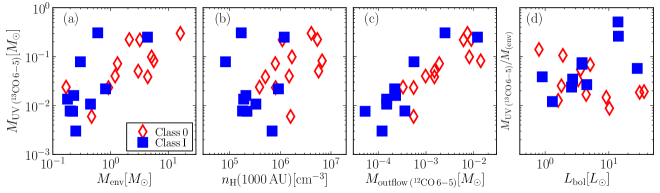
Figure 10: (a) UV heated gas mass is shown as a function of envelope mass ($M_{\rm env}$), (b) density at 1000 AU ($n_{\rm H}\,(1000\,{\rm AU})$), and (c) the outflow mass calculated from the ¹²CO 6–5 lines for the same region ($M_{\rm obs}$${}_{(^{12}{\rm CO}\,6-5)}$). (d) The fraction of the UV heated gas mass over envelope mass as a function of bolometric luminosity ($L_{\rm bol}$). Figure 10(d) has the same y-axis values as (a–c).

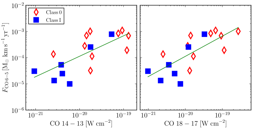
Figure 11: Correlation between $F_{\rm CO}$ and the CO 14–13 and 18–17 fluxes obtained from Herschel-PACS. The integrated intensities are scaled to a common distance of 200 pc. The green lines shows the best-fit power-laws to the data and are simple least-squares fits.

Table 5: Comparison of envelope, photon-heated and outflow masses over the 30$\times$30^′′ area surrounding the central protostar.

Source	$M_{\rm Envelope}$	$M_{\rm Envelope}$	$M_{\rm UV}$	$M_{\rm outflow}$
	Total	$\leq 15^{\prime\prime}$	13CO 6–5	12CO 6–5
L1448mm	9.0	1.69	4.0$\times$10-2	…
NGC1333-IRAS~2A	5.13	0.67	9.9$\times$10-2	8.1$\times$10-3
NGC1333-IRAS~4A	5.59	2.56	8.2$\times$10-2	1.4$\times$10-2
NGC1333-IRAS~4B	3.01	2.60	5.1$\times$10-2	2.2$\times$10-3
L1527	0.92	0.18	2.3$\times$10-2	$<$5.5$\times$10-4
Ced110-IRS4	0.17	0.07	2.4$\times$10-2	3.3$\times$10-4
IRAS~15398	0.47	0.28	6.0$\times$10-3	5.5$\times$10-4
L483mm	4.4	0.25	3.9$\times$10-2	1.5$\times$10-3
Ser-SMM1	16.13	1.99	3.0$\times$10-1	7.4$\times$10-3
Ser-SMM4	2.11	3.17	2.2$\times$10-1	8.9$\times$10-3
Ser-SMM3	3.21	0.74	2.2$\times$10-1	6.1$\times$10-3
L723mm	1.32	0.67	7.2$\times$10-2	1.9$\times$10-3
B335	1.2	0.79	4.0$\times$10-2	9.8$\times$10-4
L1489	0.18	0.04	1.4$\times$10-2	1.5$\times$10-4
TMR1	0.23	0.04	1.6$\times$10-2	2.3$\times$10-4
TMC1A	0.22	0.04	7.6$\times$10-3	5.3$\times$10-5
TMC1	0.2	0.04	7.7$\times$10-3	3.6$\times$10-4
HH46-IRS	4.36	1.21	2.5$\times$10-1	1.2$\times$10-2
DK~Cha	0.82	0.26	2.2$\times$10-2	2.2$\times$10-4
GSS30-IRS1	0.6	0.03	3.1$\times$10-1	2.5$\times$10-3
Elias~29	0.3	0.01	7.8$\times$10-2	5.6$\times$10-4
Oph-IRS63	0.25	0.12	3.0$\times$10-3	$<$1.2$\times$10-4
RNO91	0.45	0.05	1.1$\times$10-2	1.5$\times$10-4
L1551-IRS5	22.2	0.23	2.0$\times$10-2	…

4 Discussion

4.1 Mechanical feedback

Our results show that the outflow parameters inferred from the CO 6–5 data show the same trends with $L_{\rm bol}$ and evolutionary stage as found previously in the literature, but with stronger correlations than for the 3–2 data. Even though the same telescope and methods are used for all sources and the spatial resolution is high, there remains a scatter of at least an order of magnitude in the correlation between $F_{\rm CO}$ and $L_{\rm bol}$. This could point to the importance of “episodic accretion” as a resolution to the “luminosity problem” (Evans et al. 2009; Dunham et al. 2010, 2013). Some Class 0 sources are very luminous, which is likely due to a current rapid burst in accretion which may happen every 10³–10⁴ years (Dunham et al. 2010). However, their location in the high state is not constant and would drop in the course of time, on timescales as fast as 10² years (Johnstone et al. 2013). The envelope mass, on the other hand, is independent of the current luminosity, and the stronger correlation of $F_{\rm CO}$ with $M_{\rm env}$ may simply reflect that more mass is swept up.

Since the outflow force gives the integrated activity over the entire lifetime of a YSO, it is also interesting to compare this parameter with the currently shocked gas probed by the Herschel-PACS high-$J$ CO observations ($J_{\rm up}$$>$14). In Fig. 11, $F_{\rm CO}$ is plotted against CO 14–13 and CO 18–17 fluxes ($E_{\rm up}$ $\sim$580 and 940 K) obtained from Karska et al. (2013); Goicoechea et al. (2012); Herczeg et al. (2012); Green et al. (2013) and van Kempen et al. (2010a). There is a strong correlation with the CO 14–13 and CO 18–17 fluxes with $F_{\rm CO}$ ($r$=$\sim$0.76 $\sim$3.1$\sigma$; Fig. 11). This correlation illustrates that although CO 18–17 likely traces a different outflow component than CO 6–5, a component closer to the shock front (Santangelo et al. 2012; Nisini et al. 2013; Tafalla et al. 2013), the underlying driving mechanism is the same. Furthermore, CO 18–17 emission is often extended along the outflow direction (Karska et al. 2013) and clearly traces, spatially, a component related to that traced by CO 6–5. Although the excitation of CO 18–17 requires higher densities and temperatures ($n_{\rm crit}$$\sim$10⁶ cm^-3; $E_{\rm up}$$\sim$940 K) than CO 6–5 ($n_{\rm crit}$$\sim$10⁵ cm^-3; $E_{\rm up}$$\sim$120 K), CO 6–5 likely follows in the wake of the shocks traced by the higher-$J$ lines and therefore the excitation of both lines ultimately depend on the actual shock conditions. Testing this scenario requires velocity-resolved line profiles of high-$J$ lines such as CO 16–15 (Kristensen et al. in prep.).

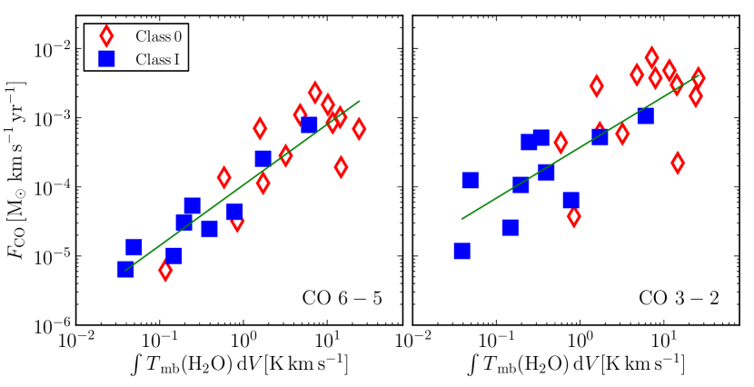
Figure 12: Correlation between $F_{\rm CO}$ measured from the CO 6–5 (left) and CO 3–2 (right) data and the integrated intensity of the ground-state H₂O 1₁₀–1₀₁ transition at 557 GHz. The integrated intensities are scaled to a common distance of 200 pc (Kristensen et al. 2012). The correlation is strong for CO 6–5, $r$=0.90 with 4.1$\sigma$. The green lines shows the best-fit power-laws to the data and are simple least-squares fits.

Another indication that the outflow force as measured from CO 6–5 is more closely linked to the currently shocked gas than that from 3–2 comes from comparing H₂O and $F_{\rm CO}$. Water is one of the best shock tracers, as shown most recently by several Herschel observations (van Kempen et al. 2010b; Lefloch et al. 2010; Kristensen et al. 2010; Nisini et al. 2010; Vasta et al. 2012; Tafalla et al. 2013). Kristensen et al. (2012) compared the integrated intensity of the H₂O 1₁₀–1₀₁ transition at 557 GHz with the outflow forces presented in the literature. These observed line intensities are scaled by the square of the source distance to a common distance of $d_{\rm avg}$=200 pc. The literature values of the outflow force used in that paper were calculated using a variety of methods and data sets, and provided an inhomogeneous sample. No correlation of H₂O integrated intensity with $F_{\rm CO}$ was found. Revisiting this comparison with the newly measured outflow forces in a consistent way reveals a correlation with the force measured from CO 3–2 data ($r$=0.78; 3.6$\sigma$) and a stronger correlation with the force measured from the CO 6–5 data ($r$=0.90; 4.1$\sigma$, Fig. 12) (see also Bjerkeli et al. 2012). Thus, $F_{\rm CO}$ as deduced from 6–5 can be used as a measure of the outflow force of the shocked gas, rather than just the entrained, swept-up gas.

4.2 Radiative feedback

The observational data demonstrate that ¹³CO 6–5 traces UV-heated gas, and that the UV-heated gas is predominantly found along the same direction as the outflow. The $A_{V}$ is lower inside the outflow cavity, because the density is lower, and so UV radiation from the accretion can escape more easily along this direction (Spaans et al. 1995; Bruderer et al. 2009; Visser et al. 2012). If there are also external UV sources, the UV-heated gas could have a more isotropic component as well but this is not traced by our ¹³CO 6–5 data at the current $S/N$ level except for the case of two sources in Ophiuchus, Elias 29 and GSS30 IRS1. Narrow ¹²CO lines may be used instead at positions well away from the outflow cone, as illustrated by previous observations (van Kempen et al. 2009b).

The estimated gas temperature of the UV-heated gas of 30–50 K is likely a lower limit to the maximum temperature achieved by this process. Model calculations by Spaans et al. (1995) and Visser et al. (2012) show that the gas temperatures can reach values up to a few hundred K at 1000 AU radius in a narrow layer along the outflow cavity, depending on source characteristics. Gas temperatures $>$30 K are maintained out to 10⁴ AU radius. Thus, in clustered environments such as NGC 1333 or Ophiuchus, it is unlikely that the gas temperature ever drops down to 10 K because the protostars heat the gas radiatively. Gas and dust temperatures are clearly decoupled, with dust temperatures significantly lower than the gas temperature, by about a factor of 2. Thus, estimates of the radiative feedback based on dust observations alone (Hatchell et al. 2013; Sicilia-Aguilar et al. 2013) likely underestimate both the temperature and the extent of the feedback. Indeed, the continuum emission, as observed with e.g. SCUBA at 450 and 850 $\mu$m, typically does not show extended structure along the direction of the outflows.

The tight correlation between the mass of the UV-heated gas and the outflow mass, when measured over the same area, is puzzling. Naively, one would expect the two properties to be unrelated as they are caused by two different physical mechanisms, UV excitation and outflow entrainment. However, the cause of these two physical processes is linked, accretion and ejection (e.g. Bontemps et al. 1996; Frank et al. 2014). The UV photons are generated in the accretion shocks onto the protostar, and during this accretion process part of the material is ejected. Thus, higher-luminosity sources at a given envelope mass should show higher UV luminosities. It is not possible to verify this hypothesis directly as all of these sources are deeply embedded. A second component is required to efficiently UV-heat the surrounding gas: an outflow cavity needs to be cleared out for the radiation to escape which requires the outflow to have been active for at least one dynamic time-scale. Thus, there may be good reason to expect a correlation between the masses of the UV-heated and outflowing gas, when measured over the same area.

5 Conclusions

In this paper, we present large-scale maps of 26 YSOs obtained with the APEX-CHAMP⁺ instrument (¹²CO and ¹³CO 6–5), together with the JCMT-HARP-B instrument (¹²CO and ¹³CO 3–2). Our sample consists of deeply embedded Class 0 sources as well as less deeply embedded Class I sources. With these high spatial and spectral resolution maps, we have studied the outflow activity of these two different evolutionary stages of YSOs in a consistent manner. All embedded sources show large-scale outflow activity that can be traced by the CO line wings, however their activity is reduced over the course of evolution to the later evolutionary stages as indicated by the decrease of several outflow parameters, including the spatial extent of the outflow as seen in the ¹²CO 6–5 maps.

One of the crucial parameters, the outflow force, $F_{\rm CO}$ is quantified and correlations with other physical parameters are sought. In agreement with previous studies, Class 0 sources have higher outflow forces than Class I sources. $F_{\rm CO}$ is directly proportional to $M_{\rm env}$ and $M_{\rm outflow}$, showing that higher outflow forces are associated with higher envelope mass and outflow mass, as present in Class 0 sources. Comparing the outflow force as measured from CO 6–5 data to H₂O observed with Herschel-HIFI and high-$J$ CO observed with Herschel-PACS reveals a correlation, suggesting that the outflow force from 6–5 is related to current shock activity. This is in contrast with the outflow force measured from CO 3–2, where the correlation with water and the high-$J$ CO fluxes is weaker.

The quiescent gas is traced by narrow (FWHM $\sim$1 km s^-1) ¹³CO 6–5 emission. For this purpose, maps are obtained in ¹³CO 6–5 transition for the sources $\sim$1^′ region around the source position. Envelope emission is modeled via radiative transfer models and is subtracted from the observed ¹³CO 6–5 emission. It is shown that an excess emission exists in most sources on scales of a 1000–2000 AU and this emission is caused by UV photons generated from the protostellar accretion process and subsequently escaping through the outflow cavities. The fraction of the UV-heated gas compared to the total envelope mass does not change from Class 0 to Class I and there are no clear signs of evolutionary trends.

UV heating is prominent along the outflow direction and this is a general observable trend. This directional preference suggests that the UV feedback on large scales is most important in the same regions as the outflows. The UV heating observed in ¹³CO 6-5 is important on scales of $<$10⁴ AU, i.e., not on cluster scales. Future models of core and disk fragmentation should take these effects into account.

Appendix A Additional Material

Table 6: Integration limits and contour levels.

		Blue Lobe			Red Lobe			CO 6–5		CO 3–2
Source	$\varv_{\rm LSR}$	$V_{\rm max}$	$V_{\rm out,blue}$	$V_{\rm in,blue}$	$V_{\rm max}$	$V_{\rm in,red}$	$V_{\rm out,red}$	Lowest Cntr	Step Size	Lowest Cntr	Step Size
	[km s-1]	[km s-1]	[km s-1]	[km s-1]	[km s-1]	[km s-1]	[km s-1]	[K km s-1]	[K km s-1]	[K km s-1]	[K km s-1]
L1448mm	$+$5.2	50.6	$-$45.4	2.0	28.8	6.6	34.0	…	…	10	10
NGC1333-IRAS 2A	$+$7.7	23.2	$-$15.5	7.0	17.3	10.5	25.0	25	20	15	15
NGC1333-IRAS 4A	$+$7.0	22.0	$-$15.5	7.0	19.8	9.2	27.0	20	20	20	20
NGC1333-IRAS 4B	$+$7.1	20.0	$-$12.8	4.0	12.8	9.2	20.0	20	20	20	20
L1527	$+$5.9	7.4	$-$1.5	4.5	8.1	7.0	14.0	7	4	5	3
Ced110-IRS4	$+$4.2	4.2	0.0	3.5	3.8	5.5	8.0	8	5	5	3
BHR71	$-$4.4	15.5	$-$20.0	$-$6.0	22.4	$-$3.9	18.0	20	20	…	…
IRAS 15398	$+$5.1	8.6	$-$3.5	4.0	9.9	6.5	15.0	5	5	3	3
L483MM	$+$5.2	10.7	$-$5.5	3.5	10.8	6.0	16.0	8	8	5	8
Ser-SMM1	$+$8.5	19.0	$-$10.5	6.0	22.5	10.5	31.0	15	20	30	25
Ser-SMM4	$+$8.0	19.0	$-$10.5	6.0	11.5	10.5	20.0	15	20	30	25
Ser-SMM3	$+$7.6	22.0	$-$13.5	6.0	13.5	10.5	22.0	15	20	30	25
L723MM	$+$11.2	14.2	$-$3.0	9.0	10.8	12.0	26.0	15	10	5	5
B335	$+$8.4	8.9	$-$0.5	7.0	8.6	9.5	17.0	5	5	…	…
L1157	$+$2.6	12.4	$-$9.8	1.5	17.4	3.7	20.0	…	…	10	20
L1489	$+$7.2	13.7	$-$6.5	5.0	7.8	8.5	15.0	3	2	10	10
L1551-IRS5	$+$6.2	9.7	$-$3.5	4.5	11.8	7.5	18.0	…	…	10	10
TMR1	$+$6.3	7.8	$-$1.5	4.0	3.7	6.5	10.0	3	3	2	2
TMC1A	$+$6.6	17.1	$-$10.5	5.0	5.4	6.5	10.0	5	5	2	5
TMC1	$+$5.2	13.7	$-$8.5	4.0	14.8	6.2	20.0	4	5	3	3
HH46-IRS	$+$5.2	5.5	$-$0.3	10.0	14.8	12.2	20.0	20	20	10	10
DK Cha	$+$3.1	5.3	$-$2.2	1.5	8.9	4.3	12.0	5	5	5	5
GSS30-IRS1	$+$3.5	13.0	$-$9.5	1.5	14.5	5.5	18.0	20	30	15	15
Elias 29	$+$4.3	9.8	$-$5.5	1.5	10.7	7.0	15.0	15	10	7.5	5.0
Oph-IRS63	$+$2.8	11.3	$-$8.5	1.0	3.2	4.0	6.0	3	1.5	2	1
RNO91	$+$0.5	15.0	$-$14.5	$-$1.0	3.5	1.0	4.0	3	3	3	3