Abstract

The elicitation of an ordinal judgment on multiple alternatives is often required in many psychological and behavioral experiments to investigate preference/choice orientation of a specific population. The Plackett-Luce model is one of the most popular and frequently applied parametric distributions to analyze rankings of a finite set of items. The present work introduces a Bayesian finite mixture of Plackett-Luce models to account for unobserved sample heterogeneity of partially ranked data. We describe an efficient way to incorporate the latent group structure in the data augmentation approach and the derivation of existing maximum likelihood procedures as special instances of the proposed Bayesian method. Inference can be conducted with the combination of the Expectation-Maximization algorithm for maximum a posteriori estimation and the Gibbs sampling iterative procedure. We additionally investigate several Bayesian criteria for selecting the optimal mixture configuration and describe diagnostic tools for assessing the fitness of ranking distributions conditionally and unconditionally on the number of ranked items. The utility of the novel Bayesian parametric Plackett-Luce mixture for characterizing sample heterogeneity is illustrated with several applications to simulated and real preference ranked data. We compare our method with the frequentist approach and a Bayesian nonparametric mixture model both assuming the Plackett-Luce model as a mixture component. Our analysis on real datasets reveals the importance of an accurate diagnostic check for an appropriate in-depth understanding of the heterogenous nature of the partial ranking data.

• Key words: Ranking data, Plackett-Luce model, Mixture models, Data augmentation, MAP estimation, Gibbs sampling, label switching, goodness-of-fit

BAYESIAN PLACKETT-LUCE MIXTURE MODELS FOR PARTIALLY RANKED DATA

dipartimento di scienze statistiche, sapienza università di roma, rome, italy

Abstract

1 Introduction

Choice behavior is a theme of great interest in several research areas, such as social and psychological sciences, but its investigation usually involves variables which cannot be directly observed and measured in an objective and precise manner. For this reason, the evidence in choice experiments is often collected in ordinal form, that is, in terms of ranking data. More specifically, ranked data arise in those studies where a sample of $N$ people is presented a finite set of $K$ alternatives, called items, and is asked to rank them according to a certain criterion, such as personal preferences or attitudes. Thus, a generic ranking is the result of a comparative judgment on the competing alternatives expressed in the form of order relation. Interest in ranked data analysis is motivated, for example, by marketing and political surveys, but also by psychological and behavioral studies consisting, for instance, in the ordering of words/topics according to the perceived association with a reference subject.

Ranked data analysis has been addressed from numerous perspectives, as revealed by a wide and consolidated literature reviewed in Marden (1995) and, more recently, in Alvo and Yu (2014). Of course, a significant role is played by the parametric modeling of ranking data, which sometimes is inspired by possible patterns underlying the (random) mechanism of formation of individual preferences. Nowadays, there is a large number of parametric ranking distributions but, despite the large availability of options, often none of them are able to embody the appropriate flexibility to represent the heterogeneous nature of real data. Consequently, it is natural to extend them to the mixture context. Our work focuses on the finite mixture approach with the Plackett-Luce model (PL) as a parametric component within a Bayesian inferential framework, aimed at analyzing heterogeneous partial rankings. It parallels the frequentist approach in Gormley and Murphy (2006). Recent works considering Bayesian mixture modeling based on the PL are Gormley and Murphy (2009) and Caron et al. (2014). Gormley and Murphy (2009) deal with a grade of membership model where, at each stage of the sequential ranking process, each sample unit has a specific partial membership of each component. This model is inherently different from the usual finite mixture model with discrete distributions on the latent variable developed in Gormley and Murphy (2006) and is better suited for soft clustering purposes. A Bayesian nonparametric PL based on a Gamma process to account for an infinite number of items, shortened as BNPPL, is developed in Caron et al. (2012). The BNPPL has been subsequently extended to the mixture context, hereinafter abbreviated as BNPPLM, by Caron et al. (2014) for analyzing clustered partial ranking data. This work relies on modeling the exchangeable sequence of random partial orderings with an infinite mixture derived by means of a stick-breaking construction of the weights, corresponding to a Dirichlet process mixture. Hence, although one can consider the BNPPLM developed by Caron et al. (2014) as a natural generalization of our finite mixture framework, we point out two important differences: (i) in our parametric setting, each single component is a standard PL for finite orderings (possibly truncated), whereas the BNPPL component models the orderings of a possibly arbitrary number of items; (ii) in our framework, the cardinality of the mixture models is explicitly defined as finite, whereas it is infinite in Caron et al. (2014). Hence, the ability of the BNPPLM to identify a suitable finite number of clusters underlying the observed data is related to the random partition associated to the sequential draw of partial rankings. In fact, for each sample unit the partial ranking is generated from the corresponding random vector of support parameters, which in turn follows a Dirichlet allocation model (McCullagh et al., 2008). Multiple sample units can then share the same parameter vector and, hence, belong to the same group of the partition. One can rely on the posterior simulation of the parameters and use, as suggested by Caron et al. (2014), the ad hoc method originally proposed by Dahl (2006) to estimate a suitable finite number of underlying groups.

In order to address the typical issues faced with a parametric finite mixture analysis, we devote special attention to alternative criteria for the determination of the appropriate number of components. Additionally, we investigate suitable diagnostic tools to detect possible deficiencies of the PL parametric class in capturing the underlying dependence structure and highlight some critical issues in combining partial orderings characterized by a different number of ranked items. Indeed, we will show how this step is relevant for an appropriate recognition of the parsimonious group structure.

The outline of the article is the following. In Section 2 we review the PL for partial orderings and its Bayesian estimation based on data augmentation. The novel Bayesian PL mixture and the related inferential procedures are presented in Section 3, together with alternative Bayesian model selection criteria and model assessment diagnostics. Illustrative applications of the proposed methods to both simulated and real ranking data are presented in Section 4. In Section 5 the paper ends with concluding remarks and hints to future developments.

2 The Plackett-Luce model

2.1 Model specification

A ranking can be elicited through a series of sequential comparisons in which a single item is preferred to all the remaining alternatives and, after being selected, is removed from the next comparisons. This is the basic construction underlying the PL, a well-established parametric distribution among the so-called stagewise ranking models. It was originally introduced by Luce (1959) and Plackett (1975). More specifically, by denoting with $K$ the total number of items to be ranked, the PL is parametrized by the support parameters $\underline{p}=(p_{1},\dots,p_{K})$ representing positive constants associated to each item: the higher the value of the support parameter $p_{i}$, the greater the probability for the $i$-th item to be preferred at each selection stage. Let $\underline{\pi}^{-1}=\{\pi_{s}^{-1}\}_{s=1}^{N}$ be a random sample consisting of $N$ partial top orderings of the form $\pi^{-1}_{s}=(\pi^{-1}_{s}(1),\dots,\pi^{-1}_{s}(n_{s}))$. With a slight abuse of notation, $n_{s}$ is the length of the $s$-th partial ordering, that is, the number of items ranked by unit $s$ in the top $n_{s}$ positions. The remaining $K-n_{s}$ items are assumed to be ranked lower. In our notation, a full ordering corresponds to the case $n_{s}=K-1$ since, once $K-1$ items have been ranked, the last position is automatically determined. Under the PL the contribution to the likelihood from the $s$-th partial ordering is given by

$$\operatorname{\mathbf{P}}_{\text{PL}}(\pi^{-1}_{s}|\underline{p})=\prod_{t=1}^{n_{s}}\dfrac{p_{\pi_{s}^{-1}(t)}}{\sum_{i=1}^{K}p_{i}-\sum_{\nu=1}^{t-1}p_{\pi_{s}^{-1}(\nu)}}.$$ (1)

We notice that for strictly partial orderings ($n_{s}<K-1$) the distribution in  (1) corresponds to the marginal PL distribution for full orderings obtained by integrating out the items ranked in the last $K-n_{s}$ positions. An important summarizing feature of $\operatorname{\mathbf{P}}_{\text{PL}}(\cdot|\underline{p})$ is the modal ordering $\sigma^{-1}_{\underline{p}}$, corresponding to the ordering of the support parameters $\underline{p}$ from the largest to the smallest.

2.2 Model estimation

The main inferential issue related to formulation (1) concerns the presence of the annoying normalization term $\left(\sum_{i=1}^{K}p_{i}-\sum_{\nu=1}^{t-1}p_{\pi_{s}^{-1}(\nu)}\right)$ that does not permit the direct maximization of the likelihood. In the maximum likelihood estimation (MLE) framework, Hunter (2004) overcomes this difficulty by applying the Minorization-Maximization algorithm, an iterative optimization method relying on the replacement of the original PL log-likelihood with a minorizing surrogate objective function. In the Bayesian perspective, instead, a related efficient solution is derived by Caron and Doucet (2012), whose work can be considered the starting point of our parametric proposal presented in the next section. In particular, Caron and Doucet (2012) propose to introduce a data augmentation step with latent quantitative variables $\underline{y}=(y_{st})$ for $s=1,\dots,N$ and $t=1,\dots,n_{s}$, whose conditional joint distribution is given by

$$f(\underline{y}|\operatorname{\underline{\pi}}^{-1},\underline{p})=\prod_{s=1}^{N}\prod_{t=1}^{n_{s}}f_{\operatorname{Exp}}\biggl{(}y_{st}\biggr{|}\sum_{i=1}^{K}p_{i}-\sum_{\nu=1}^{t-1}p_{\pi_{s}^{-1}(\nu)}\biggr{)},$$ (2)

where $f_{\operatorname{Exp}}(\cdot|\lambda)$ denotes the Negative Exponential density with rate parameter $\lambda$. The parametric assumption (2) entails remarkable simplifications for the implementation of both the posterior optimization and the Gibbs Sampling (GS) algorithm. The success of the Bayesian device introduced by Caron and Doucet (2012) is due to the combination of (2) with a conjugate prior specification. This latter aspect moves from the Thurstonian interpretation of (1), that is, Thurstone’s ranking model reduces to the PL when the Gumbel distribution is employed as distribution of the latent scores; see Yellott (1977). Caron and Doucet (2012) exploited the conjugacy of the Gamma density with the Gumbel distribution and derived a simple and effective GS scheme for the approximation of the posterior distribution.

3 Bayesian mixture of Plackett-Luce models

A wide variety of research contexts require a model-based analysis accounting for the presence of differential patterns in a collection of partially ranked data. To our knowledge, Bayesian inference of a finite PL mixture has not been previously developed in the literature concerning parametric methods to analyze such data. Bayesian PL estimation appeared so far in the literature is either limited to the homogeneous case, as in Guiver and Snelson (2009) and Caron and Doucet (2012), or accounts simultaneously for an infinite mixture configuration and an infinite number of items through a nonparametric approach; see Caron et al. (2012, 2014). In the next subsections, we detail the novel Bayesian PL mixture model for partial top rankings.

3.1 Model and prior specification

Let $\underline{\pi}^{-1}$ be a random sample of partial top orderings with varying lengths drawn from a $G$-component PL mixture, in symbols

$$\pi_{1}^{-1},\dots,\pi_{N}^{-1}|\underline{p},\operatorname{\underline{\omega}}\overset{iid}{\sim}\sum_{g=1}^{G}\omega_{g}\operatorname{\mathbf{P}}_{\text{PL}}(\pi^{-1}_{s}|\underline{p}_{g}),$$

where $\underline{p}_{g}$ is the support parameter vector specific of the $g$-th mixture component and $\omega_{g}$ is the corresponding weight. In order to suitably generalize the data augmentation approach in Caron and Doucet (2012) within the finite mixture framework, we need to introduce an additional latent feature of each generic sample unit $s$, represented by the unobserved group labels

$$\underline{z}_{s}=(z_{s1},\dots,z_{sG})|\operatorname{\underline{\omega}}\overset{iid}{\sim}\text{Multinom}(1,\operatorname{\underline{\omega}}=(\omega_{1},\dots,\omega_{G})),$$

whose univariate marginal distribution corresponds to a Bernoulli random variable (r.v.) such that

$$z_{sg}=\begin{cases}1\qquad\text{if unit $s$ belongs to the $g$-th mixture component},\\ 0\qquad\text{otherwise}.\end{cases}$$

We propose to include the unobserved group labels $\underline{z}$ in the data augmentation strategy as follows:

$$f(\underline{y}|\operatorname{\underline{\pi}}^{-1},\underline{z},\underline{p},\operatorname{\underline{\omega}})=\prod_{s=1}^{N}\prod_{t=1}^{n_{s}}f_{\operatorname{Exp}}\left(y_{st}\biggr{|}\prod_{g=1}^{G}\left(\sum_{i=1}^{K}p_{gi}-\sum_{\nu=1}^{t-1}p_{g\pi_{s}^{-1}(\nu)}\right)^{z_{sg}}\right).$$ (3)

This implies that the latent group labels determine the cluster-specific support parameters acting on the underlying quantitative variables $\underline{y}$. Once the model governing observed and latent variables is specified, a fully Bayesian approach requires the elicitation of the joint prior distribution for the unknown parameters. We choose prior distributions with independent $\underline{p}$ and $\operatorname{\underline{\omega}}$, so that $f_{0}(\underline{p},\operatorname{\underline{\omega}})=f_{0}(\underline{p})f_{0}(\operatorname{\underline{\omega}})$, and a convenient conjugate structure, similarly to the homogeneous population case. For the support parameters, in fact, we extend the initial distribution in Caron and Doucet (2012) by defining independent $p_{gi}\sim\operatorname{Ga}(c_{gi},d_{g})$, where the Gamma r.v.’s are indexed by the shape and the rate parameter. Finally, for the mixture weights, taking values in the $(G-1)$-dimensional simplex, we make the standard prior assumption $\operatorname{\underline{\omega}}\sim\operatorname{Dir}(\alpha_{1},\dots,\alpha_{G})$.

3.2 MAP estimation

In the presence of the latent variables $\underline{y}$ and $\underline{z}$, we can construct an EM algorithm in order to optimize the posterior distribution and learn the posterior mode (MAP estimate). The complete-data likelihood can be factorized as $L_{c}(\underline{p},\operatorname{\underline{\omega}},\underline{y},\underline{z})=f(\underline{y}|\operatorname{\underline{\pi}}^{-1},\underline{z},\underline{p},\operatorname{\underline{\omega}})\operatorname{\mathbf{P}}(\operatorname{\underline{\pi}}^{-1},\underline{z}|\underline{p},\operatorname{\underline{\omega}})$, that is, the product of the full-conditional (3) times the standard complete-data likelihood of a mixture model specification without data augmentation with $\underline{y}$. With simple algebra, both factors of the complete-data likelihood can be rearranged in order to explicit a multinomial form in $\underline{z}$ as follows:

$$f(\underline{y}|\operatorname{\underline{\pi}}^{-1},\underline{z},\underline{p},\operatorname{\underline{\omega}})=\prod_{s=1}^{N}\prod_{g=1}^{G}\left(\prod_{t=1}^{n_{s}}\left(\sum_{i=1}^{K}p_{gi}-\sum_{\nu=1}^{t-1}p_{g\pi_{s}^{-1}(\nu)}\right)e^{-\sum_{t=1}^{n_{s}}y_{st}\left(\sum_{i=1}^{K}p_{gi}-\sum_{\nu=1}^{t-1}p_{g\pi_{s}^{-1}(\nu)}\right)}\right)^{z_{sg}}$$

and

$$\operatorname{\mathbf{P}}(\operatorname{\underline{\pi}}^{-1},\underline{z}|\underline{p},\operatorname{\underline{\omega}})=\prod_{s=1}^{N}\prod_{g=1}^{G}\left(\omega_{g}\prod_{t=1}^{n_{s}}\dfrac{p_{g\pi_{s}^{-1}(t)}}{\sum_{i=1}^{K}p_{gi}-\sum_{\nu=1}^{t-1}p_{g\pi_{s}^{-1}(\nu)}}\right)^{z_{sg}}.$$

Hence,

$$L_{c}(\underline{p},\operatorname{\underline{\omega}},\underline{y},\underline{z})=\prod_{s=1}^{N}\prod_{g=1}^{G}\left(\omega_{g}\prod_{i=1}^{K}p_{gi}^{u_{si}}e^{-p_{gi}\sum_{t=1}^{n_{s}}\delta_{sti}y_{st}}\right)^{z_{sg}},$$

where

$$u_{si}=\begin{cases}1\quad\text{ if }i\in\{\pi_{s}^{-1}(1),\dots,\pi_{s}^{-1}(n_{s})\},\\ 0\quad\text{ otherwise},\end{cases}$$

and

$$\delta_{sti}=\begin{cases}1\quad\text{ if }i\notin\{\pi_{s}^{-1}(1),\dots,\pi_{s}^{-1}(t-1)\},\\ 0\quad\text{ otherwise},\end{cases}$$

with $\delta_{s1i}=1$ for all $s=1,\dots,N$ and $i=1,\dots,K$. We denote the complete-data log-likelihood with $l_{c}(\underline{p},\operatorname{\underline{\omega}},\underline{y},\underline{z})=\log L_{c}(\underline{p},\operatorname{\underline{\omega}},\underline{y},\underline{z})$. The implementation of the EM algorithm in the Bayesian framework iterates (i) the M-step, maximizing with respect to $(\underline{p},\operatorname{\underline{\omega}})$ the following objective function:

$$Q((\underline{p},\operatorname{\underline{\omega}}),(\underline{p}^{*},\operatorname{\underline{\omega}}^{*}))=\mathbb{E}_{\underline{y},\underline{z}|\operatorname{\underline{\pi}}^{-1},\underline{p}^{*},\operatorname{\underline{\omega}}^{*}}[l_{c}(\underline{p},\operatorname{\underline{\omega}},\underline{y},\underline{z})]+\log f_{0}(\underline{p},\operatorname{\underline{\omega}});$$

(ii) the E-step, which relies on the conditional joint distribution of all the latent variables given by

$$\operatorname{\mathbf{P}}(\underline{y},\underline{z}|\operatorname{\underline{\pi}}^{-1},\underline{p},\operatorname{\underline{\omega}})=f(\underline{y}|\operatorname{\underline{\pi}}^{-1},\underline{z},\underline{p},\operatorname{\underline{\omega}})\operatorname{\mathbf{P}}(\underline{z}|\operatorname{\underline{\pi}}^{-1},\underline{p},\operatorname{\underline{\omega}}).$$

The E-step returns

$$\begin{split}Q((\underline{p},\operatorname{\underline{\omega}}),(\underline{p}^{*},\operatorname{\underline{\omega}}^{*}))&=\sum_{s=1}^{N}\sum_{g=1}^{G}\hat{z}_{sg}\biggl{(}\log\omega_{g}+\sum_{i=1}^{K}\biggl{(}u_{si}\log p_{gi}-p_{gi}\sum_{t=1}^{n_{s}}\dfrac{\delta_{sti}}{\sum_{i=1}^{K}\delta_{sti}p^{*}_{gi}}\biggr{)}\biggr{)}\\ &\qquad+\sum_{g=1}^{G}(\alpha_{g}-1)\log\omega_{g}+\sum_{g=1}^{G}\sum_{i=1}^{K}\bigl{(}(c_{gi}-1)\log p_{gi}-d_{g}p_{gi}\bigr{)},\end{split}$$

where the posterior membership probabilities $\hat{z}_{sg}$ are obtained as

$$\hat{z}_{sg}=\dfrac{\omega_{g}^{*}\operatorname{\mathbf{P}}_{\text{PL}}(\pi^{-1}_{s}|\underline{p}_{g}^{*})}{\sum_{g^{\prime}=1}^{G}\omega_{g^{\prime}}^{*}\operatorname{\mathbf{P}}_{\text{PL}}(\pi^{-1}_{s}|\underline{p}_{g^{\prime}}^{*})}.$$

Differentiating the objective function $Q$ with respect to each $p_{gi}$ and equating to zero yields the updated support parameters of the M-step

$$p_{gi}=\dfrac{c_{gi}-1+\hat{\gamma}_{gi}}{d_{g}+\sum_{s=1}^{N}\hat{z}_{sg}\sum_{t=1}^{n_{s}}\dfrac{\delta_{sti}}{\sum_{i=1}^{K}\delta_{sti}p^{*}_{gi}}}$$

for $g=1,\dots,G$ and $i=1,\dots,K$, where $\hat{\gamma}_{gi}=\sum_{s=1}^{N}\hat{z}_{sg}u_{si}.$ Optimizing $Q$ with respect to $\operatorname{\underline{\omega}}$, subject to the canonical constraint $\sum_{g=1}^{G}\omega_{g}=1$, yields the updated mixture weights

$$\omega_{g}=\dfrac{\alpha_{g}-1+\sum_{s=1}^{N}\hat{z}_{sg}}{\sum_{g^{\prime}=1}^{G}\alpha_{g^{\prime}}-G+N}\qquad g=1,\dots,G.$$

Notice that when $G=1$ the MAP procedure collapses into the single updating formula obtained by Caron and Doucet (2012). Moreover, similarly to their method, also in our mixture approach we can recover the MLE as special case of the noninformative Bayesian analysis with flat priors, obtained by setting $c_{gi}=1$, $d_{g}=0$ and $\alpha_{g}=1$. Such a configuration of the hyperparameters, in fact, reduces the proposed MAP estimation to the algorithm described by Gormley and Murphy (2006) in the frequentist framework.

3.3 Gibbs Sampling

In order to draw a sample from the joint posterior distribution and learn about the uncertainty associated to the final estimates, we detail the implementation of a GS procedure. The conjugate prior configuration described in Section 3.1, combined with the complete-data likelihood $L_{c}(\underline{p},\operatorname{\underline{\omega}},\underline{y},\underline{z})$, leads to a sampling scheme with simple parametric distributions to be drawn from. In particular, the full-conditionals of the latent component labels are easily derived by noting that $\operatorname{\mathbf{P}}(\underline{z}|\operatorname{\underline{\pi}}^{-1},\underline{y},\underline{p},\operatorname{\underline{\omega}})\propto L_{c}(\underline{p},\operatorname{\underline{\omega}},\underline{y},\underline{z}),$ implying the following multinomial structure:

$$\operatorname{\mathbf{P}}(\underline{z}_{s}|\pi_{s}^{-1},\underline{y}_{s},\underline{p},\operatorname{\underline{\omega}})\propto\prod_{g=1}^{G}\left(\omega_{g}\prod_{i=1}^{K}p_{gi}^{u_{si}}e^{-p_{gi}\sum_{t=1}^{n_{s}}\delta_{sti}y_{st}}\right)^{z_{sg}}.$$

The full-conditionals of the support parameters are still members of the Gamma family with hyperparameters suitably updated as follows:

$$\operatorname{\mathbf{P}}(p_{gi}|\operatorname{\underline{\pi}}^{-1},\underline{y},\underline{z},p_{[-gi]},\operatorname{\underline{\omega}})\propto f_{0}(p_{gi})L_{c}(\underline{p},\operatorname{\underline{\omega}},\underline{y},\underline{z})\propto p_{gi}^{c_{gi}+\gamma_{gi}-1}e^{-p_{gi}(d_{g}+\sum_{s=1}^{N}z_{sg}\sum_{t=1}^{n_{s}}\delta_{sti}y_{st})},$$

where $\gamma_{gi}=\sum_{s=1}^{N}z_{sg}u_{si}$ is the number of units belonging to cluster $g$ who have ranked item $i$ and $p_{[-gi]}$ denotes the matrix $\underline{p}$ of the support parameters without the $(g,i)$-th entry. Also the full-conditional of the mixture weights has the same form of the corresponding prior class, obtained as

$$\operatorname{\mathbf{P}}(\operatorname{\underline{\omega}}|\operatorname{\underline{\pi}}^{-1},\underline{y},\underline{z},\underline{p})\propto f_{0}(\operatorname{\underline{\omega}})L_{c}(\underline{p},\operatorname{\underline{\omega}},\underline{y},\underline{z})\propto f_{0}(\operatorname{\underline{\omega}})\operatorname{\mathbf{P}}(\underline{z}|\operatorname{\underline{\omega}})=\prod_{g=1}^{G}\omega_{g}^{\alpha_{g}+\sum_{s=1}^{N}z_{sg}-1}.$$

Finally, the full-conditional of $\underline{y}$ is given by construction in the assumption (3).

Note that the EM and the GS can be conveniently combined by employing the MAP solution as good initialization of the chain in the MCMC simulation. However, when one adopts an MCMC procedure to derive Bayesian approximate inference of a mixture model, the MCMC sample can be affected by the annoying identifiability issue, known as label switching phenomenon (LS). This may prevent from a straightforward posterior estimation (Celeux et al., 2000; Marin et al., 2005). In the Bayesian PL mixture applications presented in Section 4 we exploited alternative relabeling algorithms that perform an ex post rearrangement of the raw MCMC drawings in order to obtain meaningful posterior estimates. These were implemented by means of the functions included in the recently released R package label.switching (Papastamoulis, 2016).

3.4 Determining the number of components

In the estimation procedures previously described, the number $G$ of groups is fixed a priori. Thus, after performing a separate inference on PL mixtures with a different number of components, a method for discriminating among the competing models is needed. In our applications, we explored three types of alternative Bayesian criteria to address this issue: (i) Deviance Information Criterion (DIC) introduced by Spiegelhalter et al. (2002), (ii) Bayesian Information Criterion-Monte Carlo (BICM) proposed by Raftery et al. (2007) and (iii) Bayesian Predictive Information Criterion (BPIC) described in Ando (2007). For an updated detailed review of Bayesian tools for model comparison, see Gelman et al. (2014). We start from the general formula $\text{DIC}=\bar{D}+p_{D}$, where $\bar{D}=\mathbb{E}[D(\theta)|\operatorname{\underline{\pi}}^{-1}]$ is the posterior expected deviance with $D(\theta)=-2\log L(\theta)$ and $p_{D}$ represents the effective number of parameters. We consider two alternative DIC formulations corresponding to two alternative ways of conceiving $p_{D}$, i.e., $\text{DIC}_{1}=\bar{D}+(\bar{D}-D(\hat{\theta}_{\text{MAP}}))$, based on the MAP estimate $\hat{\theta}_{\text{MAP}}$, and $\text{DIC}_{2}=\bar{D}+\mathbb{VAR}[D(\theta)|\operatorname{\underline{\pi}}^{-1}]/2$, suggested by Gelman et al. (2004). As shown in Raftery et al. (2007), DIC₂ coincides with AICM, that is, the Bayesian counterpart of AIC. We also use two versions of BICM, specifically $\text{BICM}_{1}=\bar{D}+\frac{\mathbb{VAR}[D(\theta)|\operatorname{\underline{\pi}}^{-1}]}{2}(\log N-1)$, which is based on the approximation of the MAP estimate from the MCMC sample (Raftery et al., 2007), and $\text{BICM}_{2}=D(\hat{\theta}_{\text{MAP}})+\frac{\mathbb{VAR}[D(\theta)|\operatorname{\underline{\pi}}^{-1}]}{2}\log N$. Finally, since one aspect often debated on DIC is its tendency to overfit, due to the double usage of the observed data, we additionally employ two BPIC formulations obtained from DIC₁ and DIC₂ by doubling their penalty term $p_{D}$.

After fitting mixture models with alternative number of components, one can select a suitable number $\hat{G}$ of components using a specific criterion and identifying the optimal mixture which minimizes that criterion. Since alternative criteria can lead to different choices, we will compare and discuss the possibly different selections of optimal models and provide some recommendation based on a simulation study.

3.5 Model assessment

Once the optimal PL mixture model has been selected, a comprehensive inferential analysis should also contemplate the adequacy of the estimated model in describing the observed data (Gelman et al., 1996). In this regard, we have focused on two important features of the ranking data $\underline{\pi}^{-1}$:

1. the most liked item frequency vector $\underline{r}(\operatorname{\underline{\pi}}^{-1})$, whose generic entry $r_{i}(\operatorname{\underline{\pi}}^{-1})=\sum_{s=1}^{N}I_{[\pi^{-1}_{s}(1)=i]}$ counts how many times item $i$ is ranked first;

2. the paired comparison frequency matrix $\tau(\operatorname{\underline{\pi}}^{-1})$, whose generic entry

   $$\begin{split}\tau_{ii^{\prime}}(\operatorname{\underline{\pi}}^{-1})=\sum_{s=1}^{N}(1-(1-u_{si})(1-u_{si^{\prime}}))I_{[\pi_{s}(i)<\pi_{s}(i^{\prime})]}=\sum_{s=1}^{N}(u_{si}+u_{si^{\prime}}-u_{si}u_{si^{\prime}})I_{[\pi_{s}(i)<\pi_{s}(i^{\prime})]}\end{split}$$

   counts the number of times that item $i$ is preferred to item $i^{\prime}$.

Within the Bayesian paradigm, it is possible to generalize the classical goodness-of-fit statistic into a parameter-dependent quantity, referred to as discrepancy variable (Gelman et al., 1996), and perform a posterior predictive check of model goodness-of-fit. Let us denote with $\operatorname{\underline{\pi}}^{-1}_{\text{obs}}$ the observed collection of partial orderings and with $\operatorname{\underline{\pi}}_{\text{rep}}^{-1}$ a replicate random draw from the posterior predictive distribution under the specified model $H$. The posterior predictive $p$ value based on a generic discrepancy variable $X^{2}(\operatorname{\underline{\pi}}^{-1};\theta)$ is defined as

$$p_{B}=\operatorname{\mathbf{P}}\left(X^{2}(\operatorname{\underline{\pi}}_{\text{rep}}^{-1};\theta)\geq X^{2}(\operatorname{\underline{\pi}}^{-1}_{\text{obs}};\theta)\biggr{|}\operatorname{\underline{\pi}}^{-1}_{\text{obs}},H\right).$$ (4)

Under correct model specification, $p_{B}$ is expected to be close to 0.5, whereas small values are deemed as an indication of model inadequacy. Here we considered 0.05 as critical threshold.

Indeed, as a first type of $X^{2}$ discrepancy measure we have considered

$$X^{2}_{(1)}(\operatorname{\underline{\pi}}^{-1};\theta)=\sum_{i=1}^{K}\frac{\left(r_{i}(\operatorname{\underline{\pi}}^{-1})-r_{i}^{*}(\theta)\right)^{2}}{r_{i}^{*}(\theta)},$$

where the symbol ^∗ indicates the theoretical frequency expected under PL mixture model with parameter $\theta=(\underline{p},\operatorname{\underline{\omega}})$. By following Yao and Böckenholt (1999), as a second discrepancy measure we have considered

$$X_{(2)}^{2}(\operatorname{\underline{\pi}}^{-1};\theta)=\sum_{i<i^{\prime}}\frac{(\tau_{ii^{\prime}}(\operatorname{\underline{\pi}}^{-1})-\tau^{*}_{ii^{\prime}}(\theta))^{2}}{\tau^{*}_{ii^{\prime}}(\theta)}.$$

Details on the computation of the posterior predictive $p$ values, denoted with $p_{B(d)}$ $d=1,2$ and corresponding to each discrepancy measure $X_{(d)}^{2}$, are reported in the Supplementary Material (SM).

Moreover, whenever partial ranking data show considerable proportions of strictly partial rankings with a different number of ranked items, one can further investigate model adequacy conditionally on the observed length of the partial orderings. This can help to verify possible violations of the underlying assumption that the subsets of rankers are identically distributed, such that their preference system is driven by the same mixture distribution on the support parameters. This check could reveal that one should better account for sample heterogeneity. To this aim, we have defined two other discrepancy measures, $\tilde{X}_{(1)}^{2}$ and $\tilde{X}_{(2)}^{2}$, which parallel the previous ones. The corresponding posterior predictive $p$ values, denoted with $\tilde{p}_{B(d)}$ $d=1,2$, allow to assess the homogeneity assumption of the strata of rankers characterized by different lengths of the expressed partial orderings. Details are reported in the SM.

4 Illustrative applications

We will apply our Bayesian model to simulated as well as two real datasets. We will verify its comparative performance with respect to some natural alternative methods, which can be expected to perform similarly, and highlight some possible advantages. We first provide some implementation details. Although the Bayesian approaches described in Section 3.2 and 3.3 permit to convey specific (subjective) prior knowledge on the parameters, in the following analyses we will rely upon weakly/noninformative prior densities with hyperparameters equal to $c_{gi}=1$, $d_{g}=.001$ and $\alpha_{g}=1$, in order to allow also for a direct comparison with the frequentist PL mixture developed by Gormley and Murphy (2006). For our parametric method, we first recorded the MAP estimate derived through the EM algorithm and subsequently employed it to initialize the GS. We run the MCMC algorithm for a total of 22000 iterations and discarded the first 2000 drawings as burn-in period. Moreover, the application of the alternative relabeling algorithms on the MCMC posterior samples revealed a good performance in removing the LS and returned very similar results in terms of adjusted estimates. Posterior means were used as final parameter estimates and those reported for the considered experiments were derived, specifically, with the application of the pivotal reordering algorithm (Marin et al., 2005).

In assessing the performance of our method, we will focus also on the comparison with the BNPPLM, since it represents the most recent natural competitor to handle heterogeneity of partial ranking data and can be expected to perform similarly. In the BNPPLM analysis, we employed the default setup for the hyperparameters described in Caron et al. (2014) and run their GS algorithm for 100000 iterations.

4.1 Simulation study

Table 1: Simulation study Percentages of top$-m$ partial orderings for the three censoring settings considered in the simulation study.

	$m$
Censoring
setting	1	2	3	4	5
A	0	2	4	10	84
B	5	15	15	20	45
C	5	20	20	25	30

We considered a simulation plan with four different PL mixture population scenarios, where the true number $G^{*}$ of components ranges from 1 to 4. Specifically, in Scenario $c\in\{1,\dots,4\}$ one has $G^{*}=c$. Under each scenario, we simulated 100 samples composed of $N=1000$ complete orderings of $K=6$ items. The values of the support parameters for each dataset were randomly generated as $p_{gi}\overset{iid}{\sim}\text{Beta}(0.3,0.3)$, where the U-shaped Beta density aims at guaranteeing a sufficient separation among the mixture components. Additionally, we assumed equal weights by setting $\omega_{g}=1/G^{*}$ for all $g=1,\dots,G^{*}$ and $G^{*}=1,\dots,4$. In order to perform the analysis on partial observations, a censoring was randomly induced on the complete orderings. In each scenario, we separately considered three censoring settings (A, B and C) for the random truncation of the complete data: the percentages of the number $m$ of top ranked items are detailed in Table 1. In censoring setting A, the percentages of partial orderings with the same number of ranked items were set equal to those observed in the CARCONF data considered in subsection 4.2. This yields approximately 16% of strictly partial orderings in each simulated sample. Censoring settings B and C are characterized by increasing proportions of truncation yielding, respectively, 55% and 70% of strictly partial observations. In this way, we are able to thoroughly explore the effectiveness of our parametric framework and its sensitivity to differential presence of strictly partial rankings in the sample. Bayesian finite PL mixtures, with a number $G$ of components ranging from 1 to 7, and the BNPPLM were fitted to all the artificial datasets for each population scenario and censoring setting. The comparison between the two models was based on the performance regarding the identification of the actual number $G^{*}$ of groups in the four scenarios. In our Bayesian parametric PL mixture analysis, the optimal number $\hat{G}$ of groups was identified by means of the alternative model selection criteria described in subsection 3.4. Tables LABEL:t:Distr1, LABEL:t:Distr2 and LABEL:t:Distr3 show the distribution of $\hat{G}$ for the alternative criteria as well as that corresponding to the BNPPLM analysis obtained with the optimization method of Dahl (2006), as suggested by Caron et al. (2014). More briefly, Table 2 displays only the agreement rates (%). Regarding censoring setting A, in Scenario 1 BPIC₁, BPIC₂ and BICM₁ always recover the actual absence of heterogeneity (i.e. $G^{*}=1$). On the other hand, this happens also for the frequentist approach employing BIC as well as for the BNPPLM. For the remaining population scenarios, BPIC₁ and DIC₁ perform from slightly to substantially better, especially in the case $G^{*}=4$ where DIC₁ emerges with an agreement rate of 81%, followed by BPIC₁ with 77%. The gap with both the frequentist and nonparametric results is considerable. BIC exhibits an agreement rate equal to 66%, whereas for BNPPLM the rate is remarkably smaller. In fact, only for 50% of the datasets BNPPLM fitted $\hat{G}=G^{*}$ components. With the application of censoring settings B and C on the same synthetic data, we faced with the situation when most of the sequences to be analyzed are partial. With both censoring settings, for $G^{*}<4$ the results associated to the Bayesian rules and BIC were found to be substantially robust with respect to censoring setting A, and DIC₁ and BPIC₁ still differ in the best agreement rates. In the case $G^{*}=4$, instead, the negative effect of the higher truncation percentage becomes more evident. In fact, we noted an overall worsening of the performance of all the selection methods, especially for the BNPPLM. Nonetheless, similarly to censoring setting A, DIC₁ exhibits the highest agreement rates (76% and 72%), confirming its sizable advantage over BIC (57% and 55%) and the BNPPLM (50% and 37%). Apparently, in almost all cases the BNPPLM approach yields the lowest agreement rates. Moreover, in the presence of heterogeneity ($G^{*}>1$), BNPPLM is consistently associated with the greatest variability regarding the determination of the number $\hat{G}$ of groups; see the corresponding distributions in Tables LABEL:t:Distr1, LABEL:t:Distr2 and LABEL:t:Distr3. If on one hand the relatively worse performance of BNPPLM is partly due to the fact that data are simulated from a different generative model, on the other it highlights a possibly substantial difference between the two approaches. Overall, our simulation study suggests to privilege the use of BPIC₁ and DIC₁ for the subsequent analysis, although with a higher occurrence of partial observations DIC₁ seems to be slightly preferable.

We conclude the simulation study by providing some evidence on the fitting measures presented in subsection 3.5. For succinctness, only results for the computation of $p_{B(d)}$ $(d=1,2)$ under the most critical population scenario with $G^{*}=4$ components are shown. Boxplots of $p_{B(d)}$ values for all the parametric PL mixtures fitted to the 100 simulated datasets are reported in Figure LABEL:fig:Diagnostic as a function of the number $G$ of fitted components. They point out the effectiveness of the proposed diagnostic tools to highlight possible deficiencies of misspecified PL mixture models. As expected, we observe an increasing trend of the posterior predictive $p$ values over $G<4$, whereas for $G\geq 4$ they stabilize around the reference value 0.5.

Table 2: Simulation study Agreement rates (%) between true number $G^{*}$ of PL components in the four population scenarios and the optimal number $\hat{G}$ of components identified, respectively, by the Bayesian PL mixture analysis via alternative model selection criteria and by the BNPPLM analysis via Dahl’s procedure. Best agreement rates for each simulation scenario and censoring setting are highlighted in bold.

Censoring setting A
$G^{*}$	DIC1	DIC2	BPIC1	BPIC2	BICM1	BICM2	BIC	BNPPLM
1	99	98	100	100	100	99	100	100
2	96	93	98	95	93	89	97	91
3	91	89	94	92	91	88	93	88
4	81	67	77	70	65	60	66	50
Censoring setting B
$G^{*}$	DIC1	DIC2	BPIC1	BPIC2	BICM1	BICM2	BIC	BNPPLM
1	99	100	100	100	100	98	100	100
2	97	93	97	98	95	89	95	89
3	92	88	94	92	90	82	92	79
4	76	61	69	65	53	48	57	50
Censoring setting C
$G^{*}$	DIC1	DIC2	BPIC1	BPIC2	BICM1	BICM2	BIC	BNPPLM
1	97	98	98	100	100	100	100	100
2	97	91	97	95	91	87	95	90
3	95	89	94	92	88	82	92	63
4	72	62	67	64	48	46	55	37

4.2 The CARCONF data

Our second analysis concerns a marketing study described in Dabic and Hatzinger (2009), aimed at investigating customer preferences toward different car features. The car configurator (CARCONF) dataset consists of $N=435$ top orderings and is available in the R package prefmod (Hatzinger and Dittrich, 2012). Customers were asked to construct their car by using an online configurator system. The respondents were presented a set of $K=6$ car modules to carry out their personal preferences, namely 1=price, 2=exterior design, 3=brand, 4=technical equipment, 5=producing country, and 6=interior design. The survey did not require a complete ranking elicitation; therefore the sample is composed of partial top orderings. The distribution of the varying number of ranked items

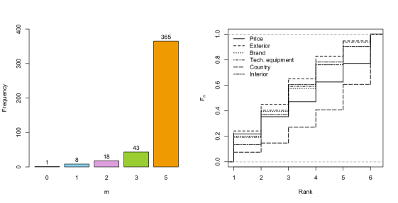
Figure 1: CARCONF data Distribution of the number $m$ of ranked items (left) and empirical c.d.f.’s of the marginal rank distributions of the car features (right).

is detailed in Figure 1 (left). Most of the customers (365 units, 84% of the sample) submitted a complete ordering of the car features. Most of the remaining customers submitted a strictly partial ordering by providing their top-4 favorite features. The vector (42,17,0,29,62,27) lists the number of missing responses for each item. Hence, all respondents assigned a rank to the brand, whereas the producing country is the one whose exact position is more frequently missing (62 occurrences corresponding to 89% of the total number of incomplete responses). The producing country is also associated with the lowest mean rank, as indicated by the fifth entry of the average rank vector $\bar{\pi}=(3.56,2.88,3.17,3.11,4.49,3.20)$. The graphical inspection of the marginal rank distribution for each item, reported in the form of empirical c.d.f. in Figure 1 (right), provides additional details on the overall preferences. We note that the c.d.f. for the producing country is remarkably stochastically dominated by the other ones, matching the idea of a minor global interest in the car production country. Another important aspect to be highlighted is the presence of intersections among the c.d.f.’s that can be interpreted as an empirical violation to the assumption of an underlying homogeneous PL, under which the rank distributions are instead expected to be marginally stochastically ordered (Marden, 1995). The observed behavior of the rank distributions could be explained with the existence of differential preference patterns in the sample. These patterns could be better captured by assuming an underlying group structure with an unknown number of groups, rather than with a basic homogeneous PL.

We estimated PL mixtures on the CARCONF data with a number of components varying from $G=1$ to $G=6$. Bayesian selection criteria and BIC are shown in Figure 2 (left). Numerical details are in Table LABEL:t:Baycrit3. BIC, as well as BICM₁ and BICM₂, does not recognize the existence of an underlying group structure despite the large sample size, whereas all versions of DIC and BPIC agree in selecting the 2-component PL mixture. The application of the BNPPLM to the CARCONF dataset agrees with the MLE inference identifying a single PL component with vector of estimated support parameters equal to $\hat{\underline{p}}=(0.123,0.231,0.195,0.193,0.071,0.187)$. In fact, the homogeneity conclusions of the ad hoc criterion in Dahl (2006) matches with the degenerate distribution of the number of distinct support parameter vectors associated to each unit across the posterior simulations. This result conflicts somehow with our preliminary descriptive findings on the violation of the stochastic dominance among the marginal rank distributions.

For all the fitted Bayesian PL mixtures, posterior predictive $p$ values are reported in the last two columns of Table LABEL:t:Baycrit3. The posterior predictive $p$ value $p_{B(2)}=0.505$ highlights a good fit in terms of the ability of the model to reproduce the bivariate features related to the pairwise comparisons, whereas $p_{B(1)}=0.079$ reveals a possible deficiency of the model to recover the marginal probability of the most favorite item, although it is larger than the usual 0.05 critical threshold. On the other hand, we notice that $p_{B(1)}<10^{-4}$ is well below for $G=1$, supporting the need of a heterogeneous model.

Parameter estimates of the optimal 2-component PL mixture are displayed in Figure 2 (center and right) and detailed in Table LABEL:t:carest. The selected mixture model suggests the presence of a major cluster ($\hat{\omega}_{1}=0.713$) comprising customers mainly interested in esthetic features, with greater support to the exterior ($\hat{p}_{12}=0.263$) rather than interior design ($\hat{p}_{16}=0.211$). The minor group ($\hat{\omega}_{2}=0.287$), instead, is characterized by a greater attention in the economic aspect represented by the price ($\hat{p}_{21}=0.436$). Both groups share a minor interest in the production country ($\hat{p}_{15}=0.071$ and $\hat{p}_{25}=0.043$). These results seem to better accord with the typical preference patterns observed in the car market than the homogeneous scenario.

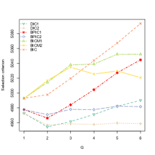
(a)

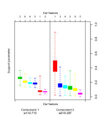
(b)

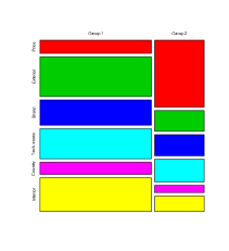
(c)

Figure 2: CARCONF data Model selection criteria (left) for the Bayesian PL mixtures with a varying number $G$ of components. For each selection criterion, the optimal choice of the number of components corresponds to the minimum value. Boxplots (center) and mosaic plot (right) for the posterior samples of the support parameters of the optimal Bayesian 2-component PL mixture.

4.3 The APA data

Another interesting dataset involving partial rankings is the popular 1980 American Psychological Association (APA) election dataset. The entire APA dataset with $N=15449$ voters ranking a maximum of $K=5$ candidates is available in the R package ConsRank.

Figure 3: APA election data Distribution of the number $m$ of ranked items (left) and distribution of the candidate occupying the first position by number of ranked items (right).

The majority of the ballots (9711, 63%) contain strictly partial orderings of the most favorite candidates and in most of them (5141, 33%) just a single favorite candidate is recorded. Some descriptive statistics are shown in Figure 3 and in the SM (Table LABEL:t:firstorder and LABEL:t:firstchoice). A detailed explanation of the data collection and the corresponding voting system yielding the elected candidate can be found in Diaconis (1987).

The popularity of these data is testified by the numerous attempts to provide an account of the complex heterogeneous structure of the ballots. From the pioneering descriptive analysis by Diaconis (1987), relying on the spectral group representation, to the most recent model-based approach by Jacques and Biernacki (2014), only few works proposed a probabilistic model for the whole set of 15449 partial orderings. Here we will show at what extent PL mixture models are able to provide an in-depth overall account of the underlying group structure.

We fitted Bayesian PL mixtures with $G=1,\dots,12$ components to the whole APA dataset. A relatively parsimonious PL mixture is selected by our parametric approach by using the Bayesian selection criteria displayed in Figure LABEL:fig:APAcriteria (numerical values are reported in Table LABEL:t:BaycritAPA). Indeed, BICM₁ and BICM₂ agree with BIC in selecting 5 components. However, as suggested in our simulation study, we privilege the use of BPIC₁ and DIC₁ which both agree in identifying $\hat{G}=10$ groups. On the other hand, the alternative BNPPLM analysis adopting Dahl’s procedure yields a partition of the electorate in 86 distinct clusters. Prior to illustrating the interpretation of the fitted components, we provide some new insights on model assessment. For the selected model, $p_{B(1)}=0.471$ and $p_{B(2)}=0.582$ do not highlight overall lack-of-fit; see Table LABEL:t:BaycritAPA. However, the substantial presence of strictly partial orderings suggested a more specific check considering the conditional distributions of the same univariate and bivariate preference features within each subset $\operatorname{\underline{\pi}}^{-1}_{m}$ of partial top orderings with the same length $m=1,\dots,4$. It revealed that the best global model fitted to the whole set of ballots is unsuitable to describe the heterogeneity of these subsets. In fact, the corresponding $\tilde{p}_{B(1)}<10^{-4}$ and $\tilde{p}_{B(2)}<10^{-4}$ are well below the conventional 0.05 critical threshold and suggest to implement our PL mixture model separately on each subset, in order to provide a more appropriate account of the heterogeneity in the APA election data. We will then compare these results with those corresponding to our initial PL mixture analysis on the entire dataset. Thus, we estimated the Bayesian PL mixture separately on top-1, top-2, top-3 and top-4 (full) orderings. Notice that on top-1 orderings only the PL mixture with $G=1$ can be fully identified, since they correspond to ordinary multinomial data on $K$ categories. Selection of the optimal number of components is displayed in Figure LABEL:fig:APAcriteria (numerical values are reported in Table LABEL:t:BaycritAPA2). Indeed, if we analyze separately each subset and comment overall on all the resulting subgroups, we get a total of $(1+2+3+7)=13$ clusters. We believe that these clusters provide a more appropriate representation of the heterogeneity in the APA election data. Unlike the overall model fitted to all the available ballots, for each model we get satisfactory fitting diagnostics (Table LABEL:t:BaycritAPA2). Now, let us focus on the support parameter estimates of the different components fitted to each subset (Figure LABEL:fig:separate). We notice that all the components exhibit distinctive modal orderings, apart from one component which shares the same modal pattern (C,A,B,E,D). Only three of them are recovered in the groups fitted to the whole dataset (Figure LABEL:fig:global). Moreover, in none of the modal orderings of the components fitted with the separate analyses Candidate B is ranked first. Instead, in two out of ten components of the global model (corresponding to a total weight 0.16) Candidate B occupies the first position of the corresponding modal ordering with a relatively large estimated support parameter. This is, to a certain extent, surprising since Candidate B is that less frequently ranked first in all the subsets; see Figure 3 (right) and the corresponding Table LABEL:t:firstchoice. Another interesting evidence from the separate analysis is that almost all components have Candidate C, D, or E in the first position of the modal orderings. The only exception, which provides maximum support to Candidate A, is found in a component fitted to the subset of full orderings. Such exceptional component, with estimated weight $\hat{\omega}_{1}=0.05$ in that subset, amounts to 1.9% of the entire dataset. Additionally, if we aggregate the relative weights of all components resulting from the separate analysis which have Candidate C (the winner of the election) in the first position of the modal ordering, we get a total weight of 0.556. The analogue computation on the global mixture returns a total weight of 0.30. Notice, however, that both analyses provide a similar posterior mean vector of the support parameters, equal to $\hat{\underline{p}}=(0.189,0.148,0.259,0.208,0.196)$ in the global analysis and $\hat{\underline{p}}=(0.192,0.148,0.257,0.206,0.197)$ with the aggregation of the separate mixtures. Finally, by looking specifically at the results of the analysis on the 5738 top-4 (full) orderings, we can compare our findings with those of previous analyses. We found a larger number of components than Diaconis (1987) and Stern (1993), both of whom identified three clusters of voters, whereas Jacques and Biernacki (2014) reported the lowest BIC for ten components, although with a similar BIC corresponding to four components. Indeed, some vectors of support parameters characterizing our group structure well compare with the findings in Stern (1993), especially those for which Candidate C is in the first position of the modal ordering. Overall, our findings allow for a characterization of the groups in terms of a more marked preference for one or two candidates.

5 Concluding remarks and future work

We have investigated a Bayesian finite PL mixture for dealing with heterogeneous partially ranked data and described efficient algorithms to conduct posterior inference. Our proposal contemplates a data augmentation step with the latent group structure and allows for model-based classification of partial top orderings. It can be seen as a direct extension to the finite mixture context of the basic Bayesian PL introduced by Caron and Doucet (2012), aimed at identifying and characterizing possible groups of rankers with similar preferences/attitudes. On the other hand, it can be regarded as a Bayesian generalization of the PL mixture developed by Gormley and Murphy (2006), whose frequentist approach can be recovered as a by-product of the noninformative analysis. An important advantage over the MLE perspective lies in the possibility to straightforwardly address estimation uncertainty, without relying on large sample approximations and additional computational burden.

We have investigated the effectiveness of our estimation algorithms in a simulation study with multiple heterogeneity scenarios. In particular, we focused on the ability to recover the actual number of clusters of the generative mixture configuration. Our Bayesian parametric proposal provided a quite satisfactory performance, even when compared with the frequentist approach as well as with the Bayesian nonparametric alternative offered by the BNPPLM in Caron et al. (2014). Our simulations highlighted sometimes remarkable divergences in the final determination of the number of clusters, possibly due to the theoretically different notion of “group” behind the two Bayesian models. The analysis of two real experiments provided further evidence on the usefulness of our parametric model. For the CARCONF data, the existence of a heterogeneous pattern of preferences emerged neither from the BNPPLM nor from the frequentist approach, whereas our proposal identified a 2-component PL mixture with two meaningful differential profiles. In general, estimating a smaller number of groups means that some preference patterns would not be recognized, leading to a less informative picture of the underlying preference system. On the other hand, the nonparametric method could prove itself more flexible to recover possible departures from the reference parametric ranking distribution by fitting a higher number of minor clusters to the sample. Summing up, both simulations and real dataset analyses highlighted that our Bayesian finite PL mixture and the BNPPLM can lead to substantially different conclusions and, sometimes, our proposal could be preferred. This happens despite the fact that the nonparametric BNPPLM method could be regarded somehow as a generalization of the Bayesian finite PL mixture.

Additionally, this work provided some incremental findings on the performance of many alternative Bayesian selection criteria. Our investigation suggests, besides the most frequently adopted DIC₁, the use of BPIC₁. Also BIC performed well for smaller values of $G^{*}$. However, for larger values of $G^{*}$ we confirm BIC’s tendency to underestimate the true number of groups, as also pointed out in other mixture settings; see for example Celeux and Soromenho (1996); Lukočienė and Vermunt (2009) and Bulteel et al. (2013). In line with this evidence, under Scenario 4 no overestimation is present with BIC; on the other hand, BIC leads to underestimate the true number $G^{*}$ of components for at least 30% of the simulated datasets in all the three censoring settings. Indeed, one could argue that, as a function of the sample size, the penalty term of BIC does not account for the varying rate of truncation, leading to a too severe penalization and, hence, to the selection of more parsimonious models. Conversely, with DIC₁ and BPIC₁ the effective number of parameters depends on the posterior deviance distribution that inherently penalizes for the increasing parameterization and the higher censoring rate. For this reason, the two Bayesian criteria could be expected to return a more adaptive and suitable estimation of model complexity. Certainly, a more theoretical advancement is needed before a clear-cut conclusion on the most suitable criterion to adopt in the finite mixture framework, where regularity conditions facilitating the derivation of asymptotic results do not hold. Indeed, apart from few recent attempts (Miller and Harrison, 2013, 2014), in the nonparametric setting the asymptotic behavior is even less explored and understood.

We also made use of diagnostic devices to evaluate the fitting of our proposal via a posterior predictive check. Despite its practical relevance, the fitting performance is often neglected by practitioners, especially in the frequentist analysis of ranking data. Unlike previous applications in the partial ranking literature, we have also applied discrepancy measures accounting for the conditional distributions, given the number of ranked items. These allow us to gain a more in-depth understanding of the adequacy of the PL parametric assumption in the whole dataset.

A possible future development could be the Bayesian estimation of the mixture of Extended PL recently introduced by Mollica and Tardella (2014). One can extend model flexibility by exploiting the additional reference order parameter, representing the rank attribution order followed by the ranker to sequentially carry out his comparative judgment on the available items. Another interesting extension could be the introduction of extra information provided by individual and/or item-specific covariates. As revealed by previous applications (Gormley and Murphy, 2008; Gormley and Murphy, 2010), explanatory variables may fruitfully contribute to characterize choice patterns and support decisions for better capturing specific preference profiles or segments. Finally, the lack-of-fit due to the differential preference patterns underlying the different subsets of rankers who provide the same number of partially ranked items highlights the need for a more comprehensive model accounting for this type of observed heterogeneity.

References

- Alvo and Yu (2014) Alvo, M. and Yu, P. L. (2014). Statistical methods for ranking data. Springer.
- Ando (2007) Ando, T. (2007). Bayesian predictive information criterion for the evaluation of hierarchical Bayesian and empirical Bayes models. Biometrika, 94(2):443–458.
- Bulteel et al. (2013) Bulteel, K., Wilderjans, T. F., Tuerlinckx, F., and Ceulemans, E. (2013). CHull as an alternative to AIC and BIC in the context of mixtures of factor analyzers. Behavior Research Methods, 45(3):782–791.
- Caron and Doucet (2012) Caron, F. and Doucet, A. (2012). Efficient Bayesian inference for Generalized Bradley-Terry models. J. Comput. Graph. Statist., 21(1):174–196.
- Caron et al. (2012) Caron, F., Teh, Y. W., and Murphy, T. B. (2012). Bayesian nonparametric Plackett-Luce models for the analysis of clustered ranked data. Technical Report 8143, Project-Team ALEA.
- Caron et al. (2014) Caron, F., Teh, Y. W., and Murphy, T. B. (2014). Bayesian nonparametric Plackett-Luce models for the analysis of preferences for college degree programmes. The Annals of Applied Statistics, 8(2):1145–1181.
- Celeux et al. (2000) Celeux, G., Hurn, M., and Robert, C. P. (2000). Computational and inferential difficulties with mixture posterior distributions. Journal of the American Statistical Association, 95(451):957–970.
- Celeux and Soromenho (1996) Celeux, G. and Soromenho, G. (1996). An entropy criterion for assessing the number of clusters in a mixture model. Journal of Classification, 13(2):195–212.
- Dabic and Hatzinger (2009) Dabic, M. and Hatzinger, R. (2009). Zielgruppenadaequate Ablaeufe in Konfigurationssystemen – Eine empirische Studie im Automobilmarkt – Partial Rankings. In Hatzinger, R., Dittrich, R., and Salzberger, T., editors, Praeferenzanalyse mit R: Anwendungen aus Marketing, Behavioural Finance und Human Resource Management. Facultas, Wien.
- Dahl (2006) Dahl, D. B. (2006). Model-based clustering for expression data via a Dirichlet process mixture model. Kim-Anh Do, Peter Müller & Marina Vannucci (Eds.), pages 201–218.
- Diaconis (1987) Diaconis, P. W. (1987). Spectral analysis for ranked data. Technical Report 282, Dept of Statistics, Stanford University.
- Gelman et al. (2004) Gelman, A., Carlin, J. B., Stern, H. S., and Rubin, D. B. (2004). Bayesian data analysis. Chapman & Hall/CRC, Boca Raton, FL, Second edition.
- Gelman et al. (2014) Gelman, A., Hwang, J., and Vehtari, A. (2014). Understanding predictive information criteria for Bayesian models. Statistics and Computing, 24(6):997–1016.
- Gelman et al. (1996) Gelman, A., Meng, X.-L., and Stern, H. (1996). Posterior predictive assessment of model fitness via realized discrepancies. Statistica Sinica, 6(4):733–760.
- Gormley and Murphy (2006) Gormley, I. C. and Murphy, T. B. (2006). Analysis of Irish third-level college applications data. Journal of the Royal Statistical Society: Series A, 169(2):361–379.
- Gormley and Murphy (2008) Gormley, I. C. and Murphy, T. B. (2008). A mixture of experts model for rank data with applications in election studies. Ann. Appl. Stat., 2(4):1452–1477.
- Gormley and Murphy (2009) Gormley, I. C. and Murphy, T. B. (2009). A grade of membership model for rank data. Bayesian Analysis, 4(2):265–295.
- Gormley and Murphy (2010) Gormley, I. C. and Murphy, T. B. (2010). Clustering ranked preference data using sociodemographic covariates. In Hess, S. and Daly, A., editors, Choice Modelling: The State-of-the-Art and the State-of-Practice: Proceedings from the Inaugural International Choice Modelling Conference, pages 543–569. Emerald.
- Guiver and Snelson (2009) Guiver, J. and Snelson, E. (2009). Bayesian inference for Plackett-Luce ranking models. In Bottou, L. and Littman, M., editors, Proceedings of the 26th International Conference on Machine Learning – ICML 2009, pages 377–384. Omnipress.
- Hatzinger and Dittrich (2012) Hatzinger, R. and Dittrich, R. (2012). prefmod: An R package for modeling preferences based on paired comparisons, rankings, or ratings. Journal of Statistical Software, 48(10):1–31.
- Hunter (2004) Hunter, D. R. (2004). MM algorithms for Generalized Bradley-Terry models. Ann. Statist., 32(1):384–406.
- Jacques and Biernacki (2014) Jacques, J. and Biernacki, C. (2014). Model-based clustering for multivariate partial ranking data. Journal of Statistical Planning and Inference, 149:201–217.
- Luce (1959) Luce, R. D. (1959). Individual choice behavior: a theoretical analysis. John Wiley & Sons Inc.
- Lukočienė and Vermunt (2009) Lukočienė, O. and Vermunt, J. K. (2009). Determining the number of components in mixture models for hierarchical data. In Advances in data analysis, data handling and business intelligence, pages 241–249. Springer.
- Marden (1995) Marden, J. I. (1995). Analyzing and modeling rank data, volume 64 of Monographs on Statistics and Applied Probability. Chapman & Hall.
- Marin et al. (2005) Marin, J.-M., Mengersen, K., and Robert, C. P. (2005). Bayesian modelling and inference on mixtures of distributions. Handbook of Statistics, 25:459–507.
- McCullagh et al. (2008) McCullagh, P., Yang, J., et al. (2008). How many clusters? Bayesian Analysis, 3(1):101–120.
- Miller and Harrison (2013) Miller, J. W. and Harrison, M. T. (2013). A simple example of Dirichlet process mixture inconsistency for the number of components. In Neural Information Processing Systems – NIPS 2013, pages 199–206.
- Miller and Harrison (2014) Miller, J. W. and Harrison, M. T. (2014). Inconsistency of Pitman-Yor process mixtures for the number of components. The Journal of Machine Learning Research, 15(1):3333–3370.
- Mollica and Tardella (2014) Mollica, C. and Tardella, L. (2014). Epitope profiling via mixture modeling of ranked data. Statistics in Medicine, 33(21):3738–3758.
- Papastamoulis (2016) Papastamoulis, P. (2016). label. switching: An R package for dealing with the Label Switching problem in MCMC outputs. Journal of Statistical Software, 69(1):1–24.
- Plackett (1975) Plackett, R. L. (1975). The analysis of permutations. Journal of the Royal Statistical Society: Series C (Applied Statistics), 24(2):193–202.
- Raftery et al. (2007) Raftery, A. E., Satagopan, Jaya, M., Newton, M. A., and Krivitsky, P. N. (2007). Bayesian statistics 8. In Bernardo, J., Bayarri, M., Berger, J., Dawid, A., Heckerman, D., Smith, A., and West, M., editors, Proceedings of the eighth Valencia International Meeting, June 2-6, 2006, pages 371–416. Oxford University Press.
- Spiegelhalter et al. (2002) Spiegelhalter, D. J., Best, N. G., Carlin, B. P., and Van Der Linde, A. (2002). Bayesian measures of model complexity and fit. Journal of the Royal Statistical Society: Series B (Statistical Methodology), 64(4):583–639.
- Stern (1993) Stern, H. (1993). Probability models on rankings and the electoral process. In Probability models and statistical analyses for ranking data, volume 80 of Lecture Notes in Statist., pages 173–195. Springer, New York.
- Yao and Böckenholt (1999) Yao, G. and Böckenholt, U. (1999). Bayesian estimation of Thurstonian ranking models based on the Gibbs sampler. British Journal of Mathematical and Statistical Psychology, 52(1):79–92.
- Yellott (1977) Yellott, John I., J. (1977). The relationship between Luce’s choice axiom, Thurstone’s theory of comparative judgment, and the double exponential distribution. J. Mathematical Psychology, 15(2):109–144.