Generalized Multiscale Finite Element Methods for problems in perforated heterogeneous domains

Abstract

Complex processes in perforated domains occur in many real-world applications. These problems are typically characterized by physical processes in domains with multiple scales (see Figure 1 for the illustration of a perforated domain). Moreover, these problems are intrinsically multiscale and their discretizations can yield very large linear or nonlinear systems. In this paper, we investigate multiscale approaches that attempt to solve such problems on a coarse grid by constructing multiscale basis functions in each coarse grid, where the coarse grid can contain many perforations. In particular, we are interested in cases when there is no scale separation and the perforations can have different sizes. In this regard, we mention some earlier pioneering works [14, 18, 17], where the authors develop multiscale finite element methods. In our paper, we follow Generalized Multiscale Finite Element Method (GMsFEM) and develop a multiscale procedure where we identify multiscale basis functions in each coarse block using snapshot space and local spectral problems. We show that with a few basis functions in each coarse block, one can accurately approximate the solution, where each coarse block can contain many small inclusions. We apply our general concept to (1) Laplace equation in perforated domain; (2) elasticity equation in perforated domain; and (3) Stokes equations in perforated domain. Numerical results are presented for these problems using two types of heterogeneous perforated domains. The analysis of the proposed methods will be presented elsewhere.

Submitted to the Special Issue Mathematical & Numerical Analysis of Flow and Transport in Porous Media

1 Introduction

Among multiscale problems, the problems in perforated domains are of great interest for many applications. The main characteristics of these problems is that the underlying processes occur in multiscale domains where the geometry of the domain has multiple scales, e.g., domain outside inclusions (see Figure 1). There are many important applications for processes in perforated domains. For example, fluid flow in porous media, diffusion in perforated domains, mechanical processes in hollow materials, and so on. Typically, it is a combination of a physical process and a heterogeneous media that gives rise to problems in perforated domains, e.g., fluid flow in porous media is a problem in perforated domain, while heat conduction in porous media may not be a problem in perforated domain.

The problems in perforated domains are of multiscale nature. The solution techniques for these problems require high resolution. In particular, the discretization needs to honor the irregular boundaries of perforations. This gives rise to a fine-scale problems with many degrees of freedom which can be very expensive to solve. In this paper, our goal is to develop coarse-grid approaches where the coarse grids do not have to align with perforations and the perforated domains do not need to have a scale separation. Our objective is to construct a low dimensional approximate model for solving fine-scale problems.

When the perforated domains have some scale separation, there are numerous works which include the works on the homogenization and asymptotic expansion in periodic perforated domains [16, 3, 4]. Recently, a novel method of meso-scale asymptotic approximation for Laplace operator is introduced ([19]) for the cases with a large number of perforations. The multiscale analysis of the perforated domain has been conducted using heterogeneous multiscale finite element method (HMMFEM) and Mulitiscale Finite Element Method (MsFEM) [16, 14, 18]. The authors in [17, 18, 20] have extended multiscale finite element methods to arbitrary perforated domains and presented novel numerical approaches using Crouzeix-Raviart coupling of multiscale finite element basis. Their approach allows perforations to intersect the boundaries of coarse-grid blocks. In their approach, the authors use oversampling technique and weak coupling via Crouzeix-Raviart to avoid directly imposing boundary conditions for the basis functions. The latter can be difficult for multiscale basis function construction in perforated domains. In our paper, we also follow this general concept and avoid constructing boundary conditions for multiscale basis functions and construct them via local spectral decomposition. Our approach follows a Generalized Mulitiscale Finite Element Method (GMsFEM) [11] in constructing multiscale basis functions which we discuss next.

GMsFEM is a general multiscale procedure where multiscale basis functions in each coarse grid are constructed and is designed for many applications [9, 6, 7]. In the GMsFEM framework, one divides the computations into two stages, i.e., the offline stage and the online stage. In the offline stage, a reduced dimensional space is constructed, and it is then used in the online stage to construct multiscale basis functions. These multiscale basis functions can be re-used for any input parameter to solve the problem on a coarse grid. The main idea behind the construction of the offline and online spaces is to design appropriate snapshot spaces and determine an appropriate local spectral problem to select important modes in the snapshot space. In [11], several general strategies for designing the local spectral procedures have been proposed. To apply GMsFEM for problems in perforated domains, one needs a novel way to construct the snapshot space and local spectral problem. In earlier works [1, 15, 13], heterogeneous problems have been studied. The main challenge is to take into account the domain heterogeneities when constructing multiscale basis functions. Compared to problems in heterogeneous media without perforated regions, we impose boundary conditions on perforations. We generate local snapshot space using harmonic extensions of appropriately chosen a large set of boundary conditions. Local spectral problems are used to select dominant modes. We also discuss the use of randomized snapshots ([2]) that allow calculating a few snapshot vectors. The latter is important in reducing the computational cost.

The above procedure is formulated for a general problem in perforated media. In this paper, we apply it to three different problems that arise in many applications. These include: (1) Laplace equation in perforated domain; (2) elasticity equation in perforated domain; and (3) Stokes equations in perforated domain. We show that our general concept can be applied to all these problems. We consider several numerical examples using two sets of perforated domains. One domain contains several large inclusions (with the sizes comparable to the coarse-grid sizes) and the other domain contains small inclusions (with the sizes much smaller than the size of the domain). We solve the above three PDEs in these two sets of domains and compare the multiscale solutions with the fine-grid solutions. Our preliminary numerical results demonstrate a fast convergence of the proposed GMsFEM approaches. In particular, we show that one can achieve a good accuracy with a very few degrees of freedom, especially for Laplace and elasticity problems. For Stokes equations, there is a room for improvement by enriching the pressure space. We discuss it in our numerical results.

The rest of the paper is organized as follows. In Section 2, we present preliminaries on the problems in perforated domains and the GMsFEM framework. The construction of the coarse spaces for the GMsFEM is discussed in Section 3. In Section 4, numerical results for several representative examples are presented. Finally, we conclude our paper with some remarks in Section 5.

2 Preliminaries

In this section, we first present the underlying problem and the corresponding fine-scale discretization. Then, we discuss the multiscale strategy of solving this problem. We consider

$$\mathcal{L}^{\varepsilon}(u)=f\quad\text{in}\quad\Omega^{\varepsilon},$$ (1)

$$u=0\text{ or }\frac{\partial u}{\partial n}=0,\text{ on }\partial\Omega^{\varepsilon}\cap\partial\mathcal{B}^{\varepsilon},$$ (2)

$$u=g,\text{ on }\partial\Omega\cap\partial\Omega^{\varepsilon}.$$ (3)

Here, $\Omega\in\mathbb{R}^{d}$ ($d=2,3$) is a bounded domain covered by inactive cells (for Stokes flow and Darcy flow) or active cells (for elasticity problem) $\mathcal{B}^{\varepsilon}$. We call active cells where the underlying problem is solved, while inactive cells being the rest of the region. Suppose the distance between inactive cells (or active cells) is at most $\varepsilon$ and we use $\epsilon$ scripts to denote the perforated domains. Denote the remaining part as $\Omega^{\varepsilon}$, i.e. $\Omega^{\varepsilon}=\Omega\backslash\mathcal{B}^{\varepsilon}$. See Figure 1 for an illustration of the perforated domain. $\mathcal{L}^{\varepsilon}$ denotes a linear differential operator, e.g. $\mathcal{L}^{\varepsilon}(u)=-\Delta u$ for Darcy flow. $n$ is the unit outward normal to the boundary and $f\in F(\Omega^{\varepsilon})$ and $g\in G(\Omega^{\varepsilon})$ denote functions with a suitable regularity. Note that $\varepsilon$ is used to denote heterogeneous domains, even though we do not assume periodicity or scale separation.

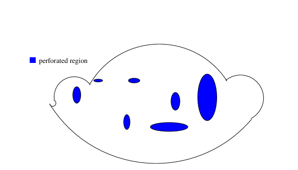
Figure 1: Illustration of a perforated domain.

To simplify the notation, we denote by ${V}(\Omega^{\varepsilon})$ the appropriate solution space, and

$${V}_{0}(\Omega^{\varepsilon})=\{v\in{V}(\Omega^{\varepsilon}),v=0\text{ on }\partial\Omega^{\varepsilon}\}.$$

The variational formulation of Problem (1) is to find $u\in{V}(\Omega^{\varepsilon})$ such that

$${\left\langle\mathcal{L}^{\varepsilon}(u),v\right\rangle}_{\Omega^{\varepsilon}}={\left\langle f,v\right\rangle}_{\Omega^{\varepsilon}}\qquad\text{for all }v\in V_{0}(\Omega^{\varepsilon}),$$

${\left\langle\cdot,\cdot\right\rangle}_{\Omega^{\varepsilon}}$ denotes a specific inner product over $\Omega^{\varepsilon}$ for either scalar functions or vector functions. In the following, we give some specific examples for the above abstract notations.

• For the Laplace operator with homogeneous Dirichlet boundary conditions on $\partial\Omega^{\varepsilon}$, we have

  $$\mathcal{L}^{\varepsilon}(u)=-\Delta u,$$ (4)

  and ${V}(\Omega^{\varepsilon})=H^{1}_{0}(\Omega^{\varepsilon})$, ${\left\langle\mathcal{L}^{\varepsilon}(u),v\right\rangle}_{\Omega^{\varepsilon}}={\left\langle\nabla u,\nabla v\right\rangle}_{\Omega^{\varepsilon}}$.

• For the elasticity operator with homogeneous Dirichlet boundary condition on $\partial\Omega^{\varepsilon}$, we let ${u}\in(H^{1}(\Omega^{\varepsilon}))^{d}$ be the displacement field. The strain tensor ${\varepsilon}({u})\in(L^{2}(\Omega^{\varepsilon}))^{d\times d}$ is defined by

  $${\varepsilon}({u})=\frac{1}{2}(\nabla{u}+\nabla{u}^{T}).$$

  In this paper, we assume the medium is isotropic. Thus, the stress tensor ${\sigma}({u})\in(L^{2}(\Omega^{\varepsilon}))^{d\times d}$ relates to the strain tensor ${\varepsilon}({u})$ in the following way

  $${\sigma}(u)=2\mu{\varepsilon}+\lambda\nabla\cdot{u}\,{I},$$

  where $\lambda>0$ and $\mu>0$ are the Lamé coefficients. We have

  $$\mathcal{L}^{\varepsilon}(u)=-\nabla\cdot{\sigma},$$ (5)

  where ${V}(\Omega^{\varepsilon})=(H^{1}_{0}(\Omega^{\varepsilon}))^{d}$ and ${\left\langle\mathcal{L}^{\varepsilon}(u),v\right\rangle}_{\Omega^{\varepsilon}}={\left\langle\sigma(u),\sigma(v)\right\rangle}_{\Omega^{\varepsilon}}$.

• For Stokes equations, we have

  $$\mathcal{L}^{\varepsilon}(u\;,p)=\begin{pmatrix}\nabla p-\mu\Delta{u}\\ \nabla\cdot{u}\end{pmatrix},$$ (6)

  where $\mu$ is the viscosity, $p$ is the fluid pressure, $u$ represents the velocity, ${V}(\Omega^{\varepsilon})=(H^{1}_{0}(\Omega^{\varepsilon}))^{d}\times L^{2}_{0}(\Omega^{\varepsilon})$, and

  $${\left\langle\mathcal{L}^{\varepsilon}(u\;,p),(v\;,q)\right\rangle}_{\Omega^{\varepsilon}}=\begin{pmatrix}{\left\langle\nabla u,\nabla v\right\rangle}_{\Omega^{\varepsilon}}&-{\left\langle\nabla\cdot v,p\right\rangle}_{\Omega^{\varepsilon}}\\ {\left\langle\nabla\cdot u,q\right\rangle}_{\Omega^{\varepsilon}}&0\end{pmatrix}.$$

  We recall that $L^{2}_{0}(\Omega^{\varepsilon})$ contains functions in $L^{2}(\Omega^{\varepsilon})$ with zero average in $\Omega^{\varepsilon}$.

We now turn our attention to a numerical approximation of the variational problem above. Due to the nature of this multiscale problem we consider the framework of multiscale finite element method [15]. The idea is computing the solution on a coarse grid instead of calculating on the fine grid directly. In the following, we introduce the necessary concepts and notations.

Let $\mathcal{T}_{H}$ be a coarse-grid partition of the domain $\Omega^{\varepsilon}$ and $\mathcal{T}_{h}$ be a conforming fine triangulation of $\Omega^{\varepsilon}$. We assume that $\mathcal{T}_{h}$ is a refinement of $\mathcal{T}_{H}$, where $h$ and $H$ represent the fine and coarse mesh sizes, respectively. Typically, we assume that $0<h\ll H<1$, and that the fine-scale mesh $\mathcal{T}_{h}$ is sufficiently fine to fully resolve the small-scale information of the domain while $H$ is a coarse mesh containing many fine-scale features. On the triangulation $\mathcal{T}_{h}$, we introduce the following finite element spaces

$${V}_{h} :=\{{v}\in V(\Omega^{\varepsilon})|{v}|_{K}\in(P^{k}(K))^{l}\mbox{ for all }K\in\mathcal{T}_{h}\},$$

where, $k=1,\;2$, $P^{k}$ denotes the polynomial approximation space, and $l=1,\;2$ indicates either a scalar or a vector.

In this paper, Generalized Multiscale Finite Element Method (GMsFEM) framework is applied. In the GMsFEM methodology, one divides the computations into offline and online computations. The offline computations are based on a preliminary dimension reduction of the fine-grid finite element spaces (that may include dealing with additionally important physical parameters, uncertainties and nonlinearities), and then the online procedure (if needed) is applied to construct a reduced order model. We start by constructing offline spaces.

We construct the coarse function space

$${V}_{\text{off}}:=\mbox{span}\{{\phi}_{i}\}_{i=1}^{N},$$

where $N$ is the number of coarse basis functions. Each ${\phi}_{i}$ is supported in some coarse neighborhood $w_{l}$ (see Figures 2 and 3 for an illustration of coarse neighborhoods).

The overall performance of the resulting GMsFEM depends on the approximation properties of the resulting offline and online coarse spaces directly. Usually, a spectral problem is involved for a good approximation of the local solution space. In this paper, we focus on the construction of the offline spaces since the differential operators $\mathcal{L}^{\varepsilon}$ is parameter independent and linear.

The GMsFEM seeks an approximation ${u}_{0}\in{V}^{\text{off}}$, which satisfies the coarse-scale offline formulation,

$${\left\langle\mathcal{L}^{\varepsilon}(u_{0}),v\right\rangle}_{\Omega^{\varepsilon}}=(f,v)_{\Omega^{\varepsilon}}\qquad\text{for all }v\in V^{\text{off}}.$$ (7)

Recall that the definitions of the bilinear forms ${\left\langle\mathcal{L}^{\varepsilon}(u_{0}),v\right\rangle}_{\Omega^{\varepsilon}}$ are defined above, and $(f,v)_{\Omega^{\varepsilon}}$ is the $L_{2}$ inner product.

We can interpret the method in the following way using matrix representations. Recall that the coarse basis functions $\{{\phi}_{i}\}^{N_{c}}_{i=1}$ are defined on the fine grid, and can be represented by the fine-grid basis functions. Specifically, we introduce the following matrices:

$$R^{T}_{0}=[{\phi}_{1},\dots,{\phi}_{N_{c}}],$$

where we identify the basis $\phi_{i}$ with their coefficient vectors on the fine-grid basis. Then, the matrix analogue of the system (7) can be equivalently written as

$$R_{0}{\left\langle\mathcal{L}^{\varepsilon}(\phi_{m}),\phi_{n}\right\rangle}_{\Omega^{\varepsilon}}R_{0}^{T}u_{0}=R_{0}F,$$ (8)

where $F$ is the fine-grid discretization of $f$. Further, once we solve the coarse system (8), we can recover the fine scale solution by $R_{0}^{T}u_{0}$. In other words, $R^{T}_{0}$ can be regarded as the transformation (also known as interpolation or downscaling) matrix from the space ${V}_{\text{off}}$ to the space ${V}_{h}$.

The accuracy of the GMsFEM relies on the coarse basis functions $\{\phi_{i}\}$. We shall present the construction of suitable basis functions for the differential operators in Section 3.

3 Local basis functions

In this section we describe the offline-online computational procedure, and elaborate on some applicable choices for the associated bilinear forms to be used in the coarse space construction. Below, we offer a general outline for the procedure.

• Offline computations:

  • 1.0. Coarse grid generation.

  • 1.1. Construction of a snapshot space that will be used to compute an offline space.

  • 1.2. Construction of a small dimensional offline space by performing dimension reduction in the space of local snapshots.

• Online computations:

  • 2.1. For each input parameter, compute multiscale basis functions (it is needed for parameter-dependent or nonlinear problems).

  • 2.2. Solve a coarse-grid problem for a forcing term and boundary condition.

  • 2.3. Iterative solvers, if needed.

In the offline computation, we first construct a snapshot space $V_{\text{snap}}^{\omega_{i}^{+}}$ or $V_{\text{snap}}^{\omega_{i}}$, depending on the choice of domain to generate the snapshot space, where $\omega_{i}^{+}$ is an oversampled region that contains a coarse neighborhood $\omega_{i}$. Construction of the snapshot space involves solving the local problems for various choices of input parameters, and we describe the details below.

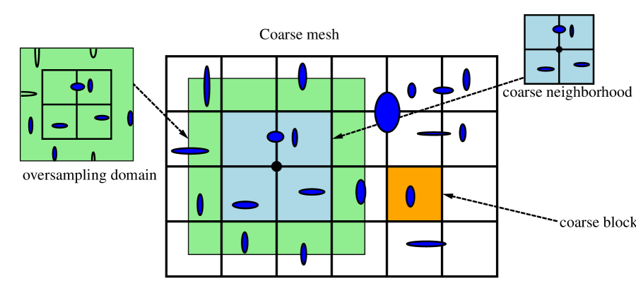
Figure 2: Illustration of a coarse neighborhood and oversampled domain

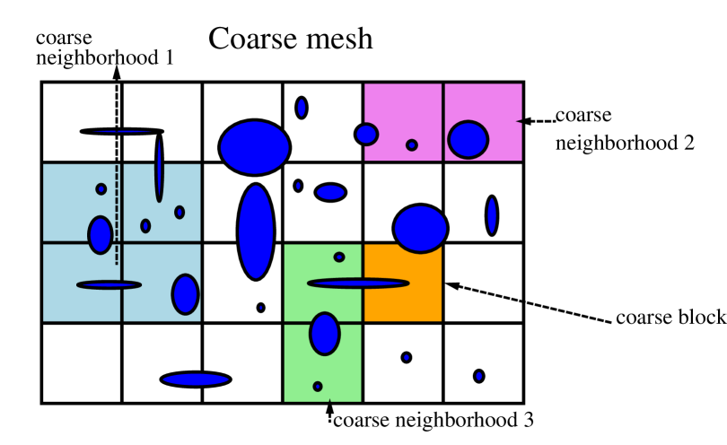
Figure 3: Illustration of a coarse neighborhood for Stokes equations

3.1 Snapshot space

First, we introduce the concept of coarse neighborhood as before. An illustration of coarse neighborhood is shown in Figures 2 and 3, respectively, for Darcy and Stokes equations. The snapshot space is composed of harmonic extension of fine-grid functions defined on the boundary of $\omega_{i}$ excluding the inactive cells in it. The local snapshots satisfy boundary conditions imposed on $\partial\mathcal{B}^{\varepsilon}$. More precisely, for each fine-grid function, $\delta_{l}^{h}(x)$, which is defined by $\delta_{l}^{h}(x)=\delta_{l,k},\,\forall l,k\in\textsl{J}_{h}(\omega_{i})$, where $\textsl{J}_{h}(\omega_{i})$ denotes the fine-grid boundary node on $\partial\omega_{i}\backslash\mathcal{B}^{\varepsilon}$.

For parameter-independent problem, we solve

$$\mathcal{L}^{\varepsilon}(\psi_{l}^{\text{snap}})=0\ \ \text{in}\ \omega_{i}\backslash\mathcal{B}^{\varepsilon}$$ (9)

subject to the boundary condition $\psi_{l}^{\text{snap}}=\delta_{l}^{h}(x)$ on $\partial\omega_{i}$ and $\psi_{l}^{\text{snap}}=0$ on $\partial\mathcal{B}^{\varepsilon}\cap\bar{\omega_{i}}$. Note that for the differential operator with Neumann boundary condition $\displaystyle\frac{\partial u}{\partial n}=0$, we will use Neumann boundary condition instead for the local problems proposed above.

We denote the space composed of $\psi_{l}^{\text{snap}}$ as

$$V_{\text{snap}}=\text{span}\{\psi_{l}^{\text{snap}}:~{}~{}1\leq l\leq M_{i}\},$$

for each coarse neighborhood $\omega_{i}$, where $M_{i}$ denotes the number of snapshots in the region $\omega_{i}$. We emphasize that an oversampling strategy (refer to Figure 2 for an illustration of oversampling domain) can be applied for the construction of snapshots to obtain a higher accuracy ([12]).

Remark 3.1.

The snapshots described above are referred to as the harmonic basis in the numerical part.

Remark 3.2.

One can also use all the fine grid functions as snapshots. These snapshots are referred to as the spectral basis in the numerical part.

3.2 Offline space

This section is devoted to the construction of the offline space via a spectral decompostion. In order to construct the offline space $V_{\text{off}}$, we perform a dimension reduction in the snapshot space using an auxiliary spectral decomposition. The main objective is to seek a subspace of the snapshot space such that it can approximate any element of the snapshot space in the appropriate sense defined via auxiliary bilinear forms. We will consider the following eigenvalue problems in the space of snapshots:

$$A^{\text{off}}\Psi_{k}^{\text{off}} = \lambda_{k}^{\text{off}}S^{\text{off}}\Psi_{k}^{\text{off}}.$$ (10)

The definitions of $A^{\text{off}}$ and $S^{\text{off}}$ for Laplace, elasticity and Stokes equations are listed below. To generate the offline space we then choose the smallest $M_{\text{off}}$ eigenvalues from Eqn. (10) and form the corresponding eigenvectors in the respective snapshot space by setting $\psi_{k}^{\text{off}}=\sum_{j}\Psi_{kj}^{\text{off}}\psi_{j}^{\text{snap}}$, for $k=1,\ldots,M_{\text{off}}$, where $\Psi_{kj}^{\text{off}}$ are the coordinates of the vector $\Psi_{k}^{\text{off}}$. We then create the offline matrices

$$R_{\text{off}}=\left[\psi_{1}^{\text{off}},\ldots,\psi_{M_{\text{off}}}^{\text{off}}\right].$$

• For Laplace operator (4),

  $$\begin{split}A^{\text{off}}=[a^{\text{off}}_{mn}]=\int_{\omega_{i}\backslash\mathcal{B}^{\varepsilon}}\nabla\psi_{m}^{\text{snap}}\cdot\nabla\psi_{n}^{\text{snap}},\text{ and }\\ S^{\text{off}}=[s^{\text{off}}_{mn}]=\int_{\omega_{i}\backslash\mathcal{B}^{\varepsilon}}\psi_{m}^{\text{snap}}\psi_{n}^{\text{snap}}.\end{split}$$ (11)

• For elasticity operator (5),

  $$\begin{split}A^{\text{off}}=[a^{\text{off}}_{mn}]=\int_{\omega_{i}\backslash\mathcal{B}^{\varepsilon}}\Big{(}2\mu{\varepsilon}(\psi_{m}^{\text{snap}}):{\varepsilon}(\psi_{n}^{\text{snap}})+\lambda\nabla\cdot{\psi_{m}^{\text{snap}}}\,\nabla\cdot\psi_{n}^{\text{snap}}\Big{)}\;,\text{ and }\\ \displaystyle S^{\text{off}}=[s^{\text{off}}_{mn}]=\int_{\omega_{i}\backslash\mathcal{B}^{\varepsilon}}(\lambda+2\mu)\psi_{m}^{\text{snap}}\cdot\psi_{n}^{\text{snap}}.\end{split}$$ (12)

• For Stokes operator (6),

  $$\begin{split}A^{\text{off}}=[a^{\text{off}}_{mn}]=\int_{\omega_{i}\backslash\mathcal{B}^{\varepsilon}}\nabla\psi_{m}^{\text{snap}}:\nabla\psi_{n}^{\text{snap}},\text{\text{and}}\\ \displaystyle S^{\text{off}}=[s^{\text{off}}_{mn}]=\int_{\omega_{i}\backslash\mathcal{B}^{\varepsilon}}\psi_{m}^{\text{snap}}\cdot\psi_{n}^{\text{snap}}.\end{split}$$ (13)

  Note that for the Stokes operator, multiscale spaces are constructed for velocity field only, and we use piecewise constant approximation on the coarse grid for the pressure.

We remark that some adaptive procedures for choosing the offline basis are proposed and analyzed in [10, 8]. In our future work, we plan to present an analysis of the method which can guide us in choosing the local spectral problems.

4 Simulation results

In this section, we present simulation results using the framework presented in Section 3 for Laplace equation, elasticity equation and Stokes equations, respectively. We set $\Omega=[0,1]\times[0,1]$ and use two types of perforated domains as illustrated in Figure LABEL:fig:domain, where the perforated regions $\mathcal{B}^{\varepsilon}$ are circular. Note that we can also use perforated regions of other shapes instead and obtained similar results. The computational domain is discretized coarsely using uniform triangulation as shown in the left of Figures 5 and 6, where the coarse mesh size $H={1\over 5}$. Furthermore, nonuniform triangulation is used inside each coarse triangle element to obtain a finer discretization. Examples of this triangulation are displayed on the right of Figures 5 and 6, where $2188$ and $2364$ nonuniform triangle elements are generated, respectively.

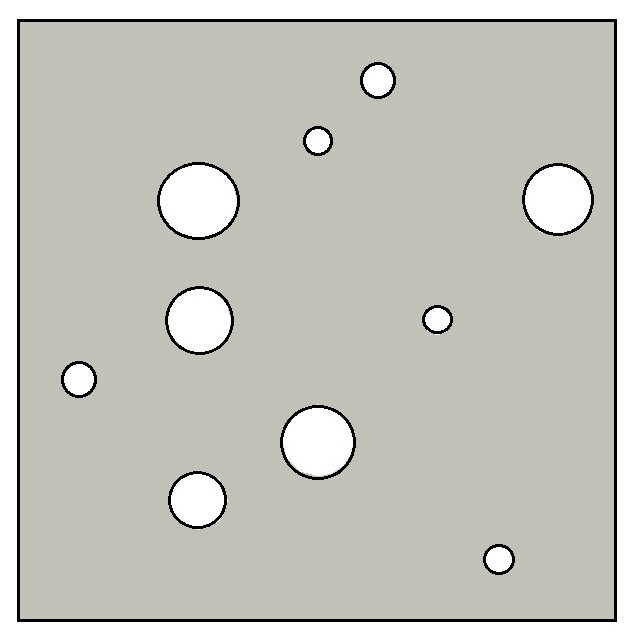
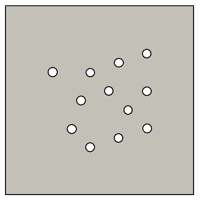
Figure 4: Two heterogeneous perforated medium used in the simulations.

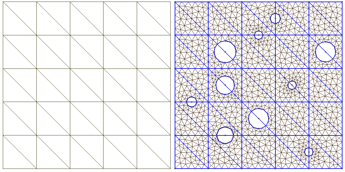
Figure 5: Coarse-scale and fine-scale discretization corresponds to the heterogeneous medium on the left of Figure LABEL:fig:domain.

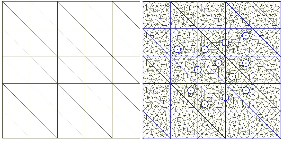
Figure 6: Coarse-scale and fine-scale discretization corresponds to the heterogeneous medium on the right of Figure LABEL:fig:domain.

4.1 Laplace equation in perforated domain

First, we consider the Laplace operator (4) imposed with zero Dirichlet boundary condition on the holes $\partial\Omega^{\varepsilon}\cap\partial\mathcal{B}^{\varepsilon}$ and $u=1$ on $\partial\Omega$, and $f=0$.

The simulation results in perforated domains as shown in Figure LABEL:fig:domain are illustrated in Figures 7 and 8, respectively. The multiscale solution is obtained in an offline space of dimension $432$ (using $12$ basis functions per coarse neighborhood) and the fine-scale reference solution is obtained in a space of dimension $1187$. Compared the fine-scale solution on the left with the coarse-scale solution on the right of the figures, we observe that the GMsFEM can approximate the fine-scale solution accurately.

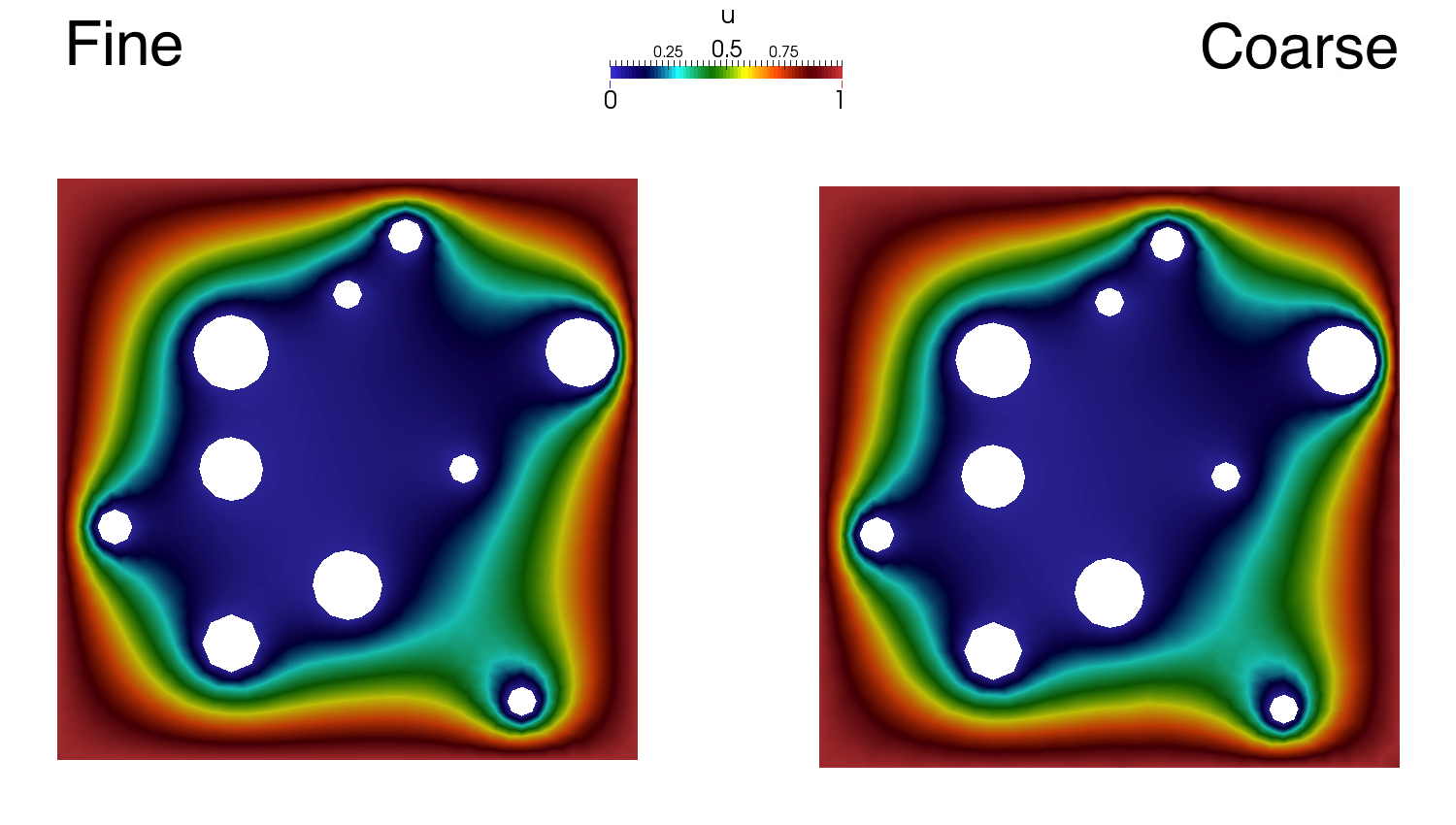
Figure 7: Fine-scale and coarse-scale solution to the Laplace equation in the heterogeneous medium on the left of Figure LABEL:fig:domain. The dimension of the coarse space is 432.

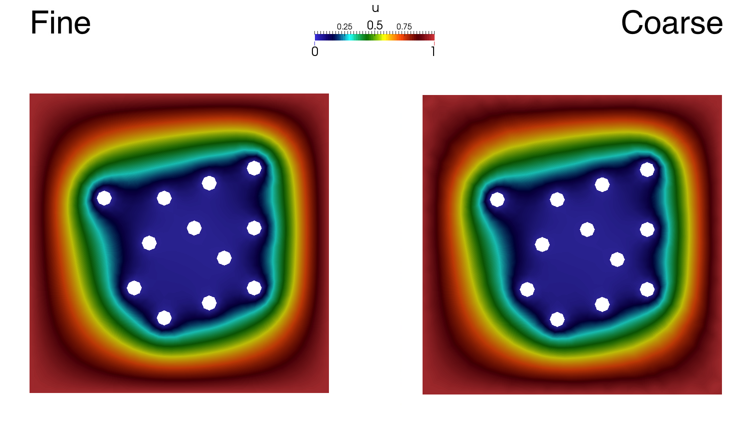
Figure 8: Fine-scale and coarse-scale solution to the Laplace equation in the heterogeneous medium on the right of Figure LABEL:fig:domain. The dimension of the coarse space is 432.

Besides, two types of snapshot spaces are applied in our simulations with the results shown in Tables 1 and 2. The first column of each table shows the number of basis in each coarse node ($N_{c}$). The dimensions of the offline spaces are given in the second column. The next two columns display the $L_{2}$ and $H_{1}$ relative errors for using spectral basis. We can see that the $L_{2}$ and $H_{1}$ relative errors are $0.2\%$ and $2\%$ respectively when the dimension of the coarse space is $432$. The results applying harmonic extenstion type of basis (Eqn. (9)) are listed in the last two columns. As displayed in Table 1, the $L_{2}$ and $H_{1}$ relative errors are $1\%$ and $17\%$ respectively when the dimension of the coarse space is $432$. Note that the GMsFEM gives a very good solution in both cases with only about $36\%$ of unknown compared to the fine-scale solver. We also observe in Tables 1 and 2 that a rapid decay in the errors as we increase the number of basis functions.

$N_{c}$	dim	harmonic basis		spectral basis
		$L_{2}$	$H_{1}$	$L_{2}$	$H_{1}$
1	36	0.18	0.75	0.19	0.63
2	72	0.12	0.65	0.10	0.45
4	144	0.06	0.48	0.02	0.18
8	288	0.03	0.35	0.01	0.09
12	432	0.01	0.17	0.002	0.02
16	576	0.004	0.04	0.001	0.009

Table 1: Numerical tests for Laplace operator in heterogeneous medium shown on the left of Figure LABEL:fig:domain. Fine-scale problem dimension is 1187.

$N_{c}$	dim	harmonic basis		spectral basis
		$L_{2}$	$H_{1}$	$L_{2}$	$H_{1}$
1	36	0.10	0.89	0.06	0.34
2	72	0.09	0.88	0.03	0.25
4	144	0.05	0.65	0.01	0.10
8	288	0.03	0.52	0.005	0.05
12	432	0.01	0.29	0.001	0.02
16	576	0.003	0.06	0.0006	0.009

Table 2: Numerical tests for Laplace operator in heterogeneous medium shown on the right of Figure LABEL:fig:domain. Fine-scale problem dimension is 1269.

4.2 Elasticity equation in perforated domain

Next, we consider elasticity operator (5). We use zero displacements $u=0$ on the holes, $u_{x}=0,\sigma_{y}=0$ on the left boundary, $\sigma_{x}=0,u_{y}=0$ on the bottom boundary and $\sigma_{x}=0,\sigma_{y}=0$ on the top and right boundaries. Here, $u=(u_{x},u_{y})$ and $\sigma=(\sigma_{x},\sigma_{y})$. The source term is defined by $f=(10^{7},10^{7})$, the elastic modulus is given by $E=10^{9}$, Poisson’s ratio is $\nu=0.22$, where

$$\mu=\frac{E}{2(1+\nu)},\quad\lambda=\frac{E\nu}{(1+\nu)(1-2\nu)}.$$

The fine-scale solution and coarse-scale solution corresponding to different perforated domains in Figure LABEL:fig:domain are presented in Figures 9 and 10. The fine-scale displacement is displayed on the left, while the coarse-scale displacement is displayed on the right. The multiscale solution is obtained in an offline space of dimension $864$ (using $12$ basis functions per coarse neighborhood for each component of the displacement) and the fine-scale reference solution is obtained in a space of dimension $2374$. Comparing the fine-scale solution with the coarse-scale solution in Figures 9 and 10, we can observe a good accuracy.

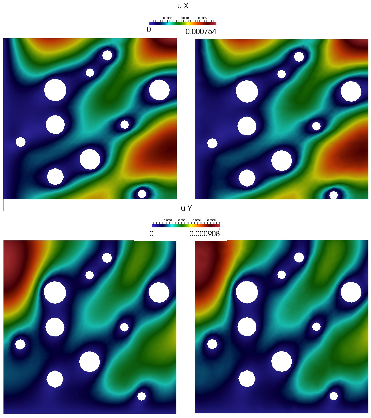
Figure 9: The fine-scale and coarse-scale solutions of the elasticity equation correspond to the heterogeneous perforated domain shown on the left of Figure LABEL:fig:domain. The dimension of the fine-scale solution is 2374 and the dimension of the coarse space is 864.

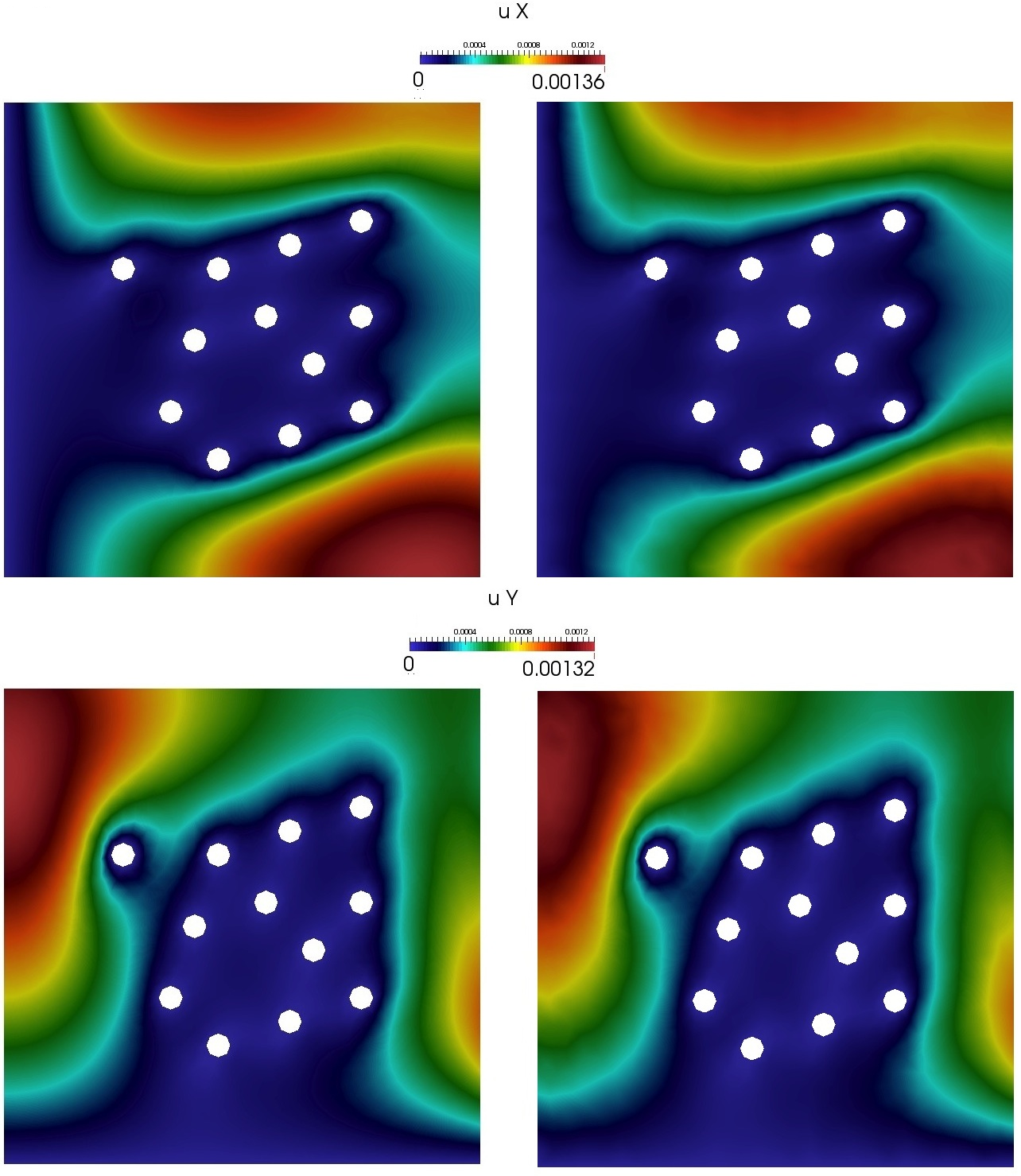
Figure 10: The fine-scale and coarse-scale solutions of the elasticity equation correspond to the heterogeneous perforated domain shown on the right of Figure LABEL:fig:domain. The dimension of the fine-scale solution is 2538 and the dimension of the coarse space is 900.

Furthermore, the relative errors for different dimensions of coarse spaces with harmonic basis functions (Eqn. (9)) and spectral basis functions are shown in Tables 3 and 4, respectively. As displayed in Table 3, the $L_{2}$ and $H_{1}$ relative errors using harmonic basis are $3\%$ and $14\%$, respectively, when the dimension of the coarse space is $1152$ for the perforated domain shown in the left of Figure LABEL:fig:domain. In addition, for the same dimension of the coarse space and the same domain, the $L_{2}$ and $H_{1}$ relative errors using spectral basis are $0.5\%$ and $5\%$, respectively Note that the dimension of the fine-scale solution is 2374. Thus, we see that the proposed GMsFEM gives accurate solutions. We also observe that GMsFEM gives more accurate solution when more basis are included in the offline space. We remark that the results (see Table 4) follow a similar pattern for the domain shown on the right of Figure LABEL:fig:domain.

$N_{c}$	dim	harmonic basis		spectral basis
		$L_{2}$	$H_{1}$	$L_{2}$	$H_{1}$
1	72	0.65	0.74	0.58	0.75
2	144	0.41	0.57	0.21	0.46
4	288	0.32	0.48	0.07	0.26
8	576	0.16	0.32	0.02	0.13
12	864	0.11	0.25	0.009	0.08
16	1152	0.03	0.14	0.005	0.05
20	1440	0.01	0.04	0.003	0.03

Table 3: Numerical tests for elasticity equations in heterogeneous medium shown on the left of Figure LABEL:fig:domain. The fine-scale problem dimension is 2374.

$N_{c}$	dim	harmonic basis		spectral basis
		$L_{2}$	$H_{1}$	$L_{2}$	$H_{1}$
1	72	0.79	0.86	0.65	0.81
2	144	0.53	0.69	0.11	0.35
4	288	0.45	0.62	0.04	0.20
8	576	0.22	0.41	0.01	0.12
12	864	0.16	0.34	0.007	0.07
16	1152	0.06	0.20	0.003	0.05
20	1440	0.01	0.12	0.002	0.04

Table 4: Numerical tests for elasticity equations in heterogeneous medium shown on the right of Figure LABEL:fig:domain. The fine-scale problem dimension is 2538.

4.3 Stokes equations in perforated domain

In our final example, we consider the Stokes operator (6) with zero velocity $u=(0,0)$ on $\partial\Omega^{\varepsilon}\cap\partial\mathcal{B}^{\varepsilon}$ and $u=(1,0)$ on $\partial\Omega$. The numerical results corresponding to different perforated domains in Figure LABEL:fig:domain are listed in Figures 11 and 12. The fine-scale solution and coarse-scale solution are depicted on the left and right of Figures 11 and 12, respectively. To improve the accuracy, we have enriched pressure spaces by considering a splitting algorithm [5]. Our preliminary numerical results show an improvement.

$N_{c}$	dim	harmonic basis
		$L_{2}$	$H_{1}$
1	108	0.85	0.88
2	180	0.68	0.78
4	324	0.40	0.69
8	612	0.26	0.67
12	900	0.23	0.60
16	1188	0.23	0.58

Table 5: Numerical tests for Stokes operator in heterogeneous medium shown on the left of Figure LABEL:fig:domain. Fine-scale problem dimension is 3561.

$N_{c}$	dim	harmonic basis
		$L_{2}$	$H_{1}$
1	108	0.65	0.87
2	180	0.56	0.82
4	324	0.31	0.71
8	612	0.16	0.62
12	900	0.13	0.46
16	1188	0.13	0.44

Table 6: Numerical tests for Stokes operator in heterogeneous medium shown on the right of Figure LABEL:fig:domain. Fine-scale problem dimension is 3807.

The $L_{2}$ and $H_{1}$ relative errors in different perforated domains in Figure LABEL:fig:domain are listed in Tables 5 and 6, respectively. We observe that the $L_{2}$ and $H_{1}$ relative errors are $23\%$ and $58\%$, respectively. As more basis are taken in the construction of the offline space, the $L_{2}$ and $H_{1}$ relative errors become smaller. In general, enriching pressure spaces and constructing associated velocity spaces can improve the accuracy. This is currently under investigation.

Figure 11: The fine-scale and coarse-scale solutions of the pressure, x-component and y-component of the velocity correspond to the heterogeneous perforated domain shown on the left of Figure LABEL:fig:domain. The dimension of the fine-scale solution is 3561.

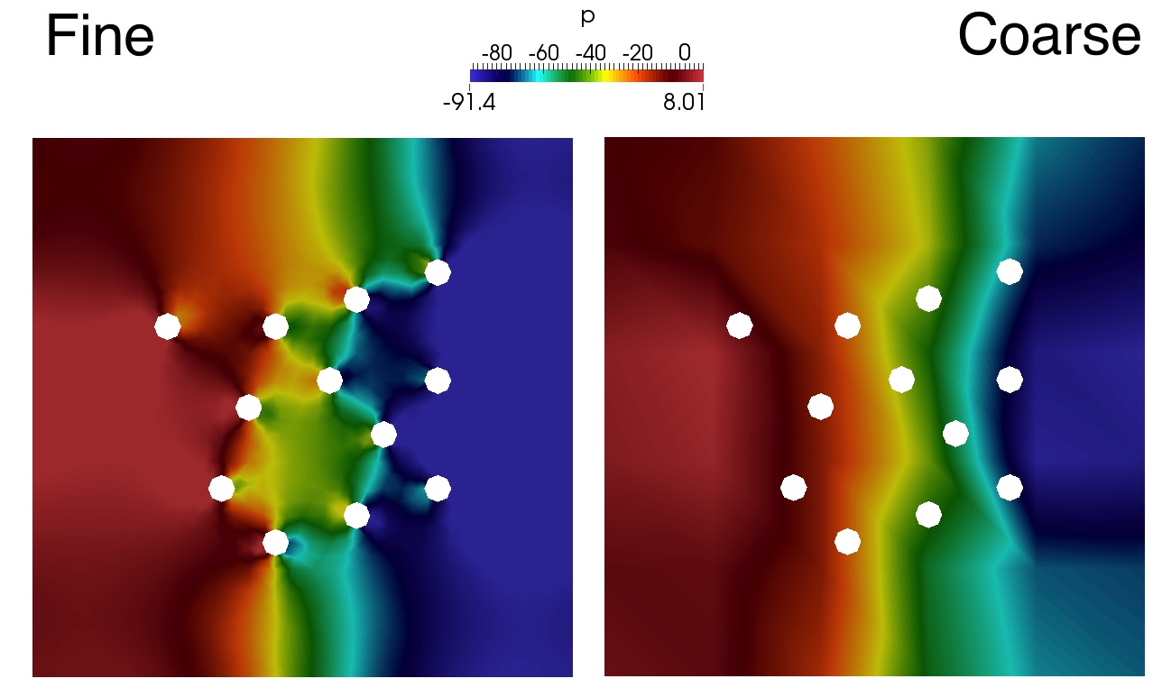
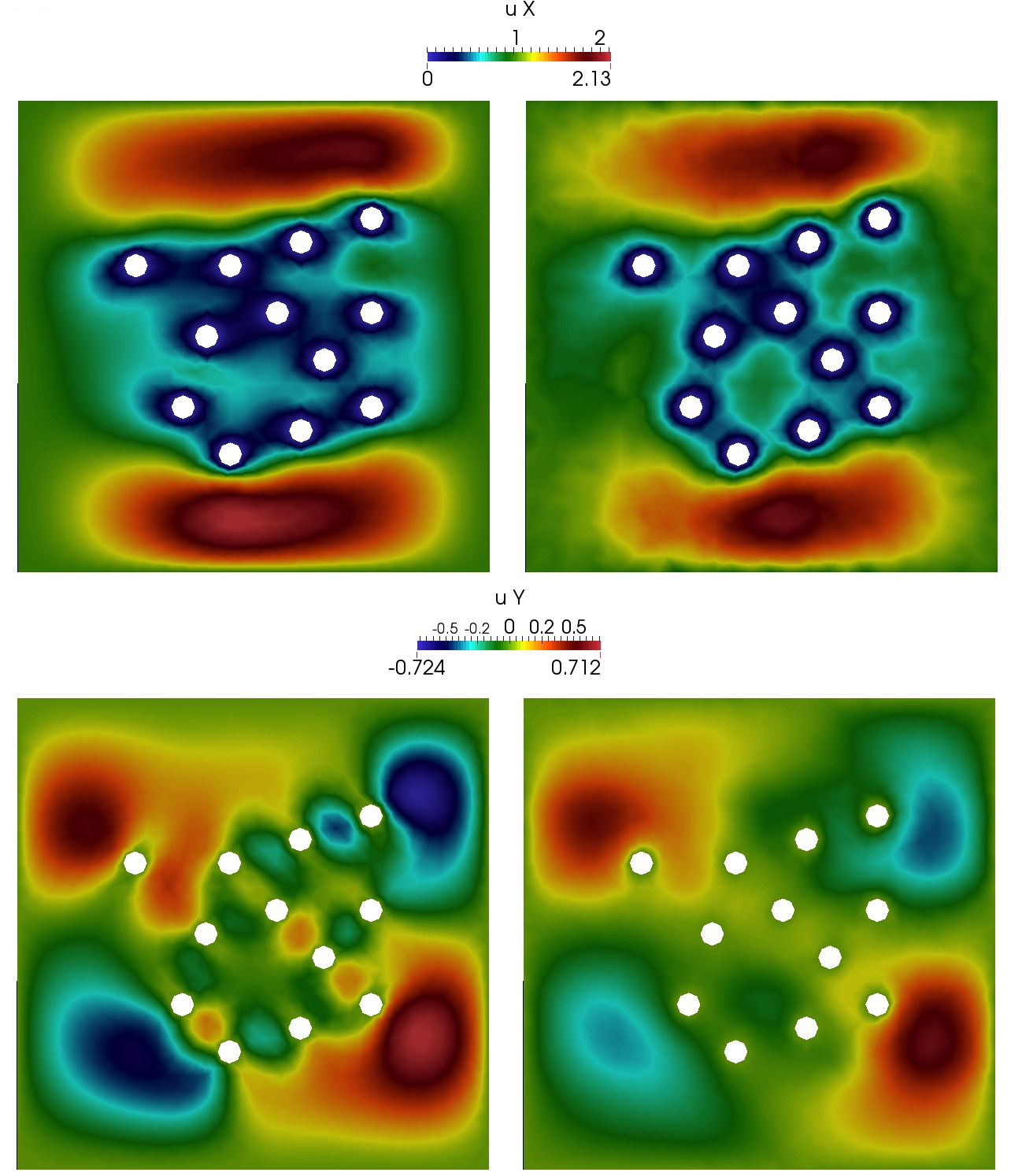
Figure 12: The fine-scale and coarse-scale solutions of the pressure, x-component and y-component of the velocity correspond to the heterogeneous perforated domain shown on the right of Figure LABEL:fig:domain. The dimension of the fine-scale solution is 3807.

4.4 Randomized snapshots for GMsFEM

In this subsection, we will investigate the oversampling randomized algorithm proposed in [2] (shown in Table 7). The advantage of this algorithm lies in the fact that a much fewer number of snapshot basis functions are calculated maintaining a good accuracy to the solution space concurrently. Besides, the oversampling strategy is used to reduce the mismatching effects of boundary conditions imposed artificially in the construction of snapshot basis functions. For the sake of brevity, the results for elasticity equation are shown only.

The simulation results are presented in Tables 8 and 9 for elasticity problem. The results without oversampling are shown on the top of each table, while those with the oversampling strategy are shown on the bottom part of each table. In our simulation, we set the oversampling size $t=2$ (i.e., two extra fine-grid blocks are added to the original coarse region) and a buffer number $p_{\text{bf}}^{\omega_{i}}=4$ for each coarse neighborhood $\omega_{i}$, i.e., we will generate 4 more snapshot basis functions in each coarse neighborhood. In the numerical results, we report the fraction of the snapshots computed compared to all snapshot vectors. For the sake of completeness, we list the algorithm in Table 7.

Table 7: Randomized GMsFEM Algorithm

Input:	Fine grid size $h$, coarse grid size $H$, oversampling size $t$, buffer number $p_{\text{bf}}^{\omega_{i}}$ for each $\omega_{i}$,
	the number of local basis functions $k_{\text{nb}}^{\omega_{i}}$ for each $\omega_{i}$;
output:	Coarse-scale solution $u_{H}$.
1.	Generate oversampling region for each coarse block: $\mathcal{T}^{H}$, $\mathcal{T}^{h}$, and $\omega_{i}^{+}$;
2.	Generate $k_{\text{nb}}^{\omega_{i}}+p_{\text{bf}}^{\omega_{i}}$ random vectors $r_{l}$ and obtain randomized snapshots in $\omega_{i}^{+}$;
	Add a snapshot that represents the constant function on $\omega_{i}^{+}$;
3.	Obtain $k_{\text{nb}}^{\omega_{i}}$ offline basis by a spectral decomposition restricted to the original region;
4.	Construct multiscale basis functions and solve it.

$N_{c}$	full snapshots		randomized snapshots
	$L_{2}$	$H_{1}$	$L_{2}$	$H_{1}$
without oversampling, $w_{i}$
	100 %		39.7 %
1	0.572	0.753	0.764	0.853
2	0.217	0.466	0.592	0.742
4	0.071	0.261	0.317	0.529
8	0.023	0.136	0.173	0.386
12	0.009	0.079	0.101	0.286
16	0.005	0.054	0.055	0.214
with oversampling, $w^{+}_{i}=w_{i}+2$
	100 %		25.2 %
1	0.506	0.716	0.533	0.729
2	0.223	0.472	0.203	0.450
4	0.069	0.258	0.065	0.252
8	0.025	0.143	0.025	0.146
12	0.010	0.083	0.013	0.095
16	0.006	0.058	0.007	0.069

Table 8: Numerical tests for elasticity in heterogeneous media shown on the left of Figure LABEL:fig:domain. Randomized oversampling for GMsFEM.

$N_{c}$	full snapshots		randomized snapshots
	$L_{2}$	$H_{1}$	$L_{2}$	$H_{1}$
without oversampling, $w_{i}$
	100 %		39.2 %
1	0.692	0.822	0.858	0.908
2	0.116	0.351	0.673	0.798
4	0.039	0.207	0.510	0.678
8	0.016	0.128	0.358	0.551
12	0.007	0.078	0.204	0.418
16	0.003	0.055	0.132	0.334
with oversampling, $w^{+}_{i}=w_{i}+2$
	100 %		23.3 %
1	0.665	0.800	0.611	0.762
2	0.115	0.355	0.131	0.383
4	0.038	0.214	0.049	0.241
8	0.015	0.135	0.020	0.157
12	0.006	0.087	0.008	0.108
16	0.006	0.089	0.008	0.102

Table 9: Numerical tests for elasticity in heterogeneous media shown on the right of Figure LABEL:fig:domain. Randomized oversampling for GMsFEM.

Comparing the results on the left columns (using full snapshot space) of Tables 8 and 9 with those on the right columns that correspond to the randomized snapshots, we observe that the randomized algorithm provides a nearly similar results, particularly with oversampling strategy. This is consistent with our previous observations for heterogeneous problems. Oversampling avoids the oscillations on the boundary conditions due to the randomness. The effect of oversampling strategy is much more obvious for the randomized snapshot space.

5 Conclusion

In this paper, we develop a generalized multiscale finite element framework for problems in perforated domains. Our approach follows GMsFEM. The main contributions of this paper are the development of snapshot space and local spectral problems for solving problems in perforated domains with multiple scales and no scale separation. Our approaches differ from previously developed GMsFEM techniques for heterogeneous problems. In particular, the snapshot vectors and local eigenvalue problems need to be developed in a multiscale domain and take into account the boundaries that may be disconnected. We show that using GMsFEM framework, we can propose a unified framework for solving problems in perforated domains. In the paper, we discuss three applications: (1) Laplace equation in perforated domain; (2) elasticity equation in perforated domain; and (3) Stokes equations in perforated domain. We present some preliminary numerical results that show that one can efficiently solve these problems on a coarse grid using fewer degrees of freedom. We also discuss the use of randomized snapshots to reduce the offline computational cost associated with computing the snapshot space. In our future work, we plan to present analysis and design new more efficient coarse spaces based on the analysis.

6 Acknowledgement

YE’s work is partially supported by the U.S. Department of Energy Office of Science, Office of Advanced Scientific Computing Research, Applied Mathematics program under Award Number DE-FG02-13ER26165 and the DoD Army ARO Project.

References

- [1] I. Babuška, V. Nistor, and N. Tarfulea, Generalized finite element method for second-order elliptic operators with Dirichlet boundary conditions, J. Comput. Appl. Math., 218 (2008), pp. 175–183.
- [2] V. Calo, Y. Efendiev, J. Galvis, and G. Li, Randomized oversampling for generalized multiscale finite element methods, Submitted. arXiv:1409.7114.
- [3] L. Cao, Multiscale asymptotic expansion and finite element methods for the mixed boundary value problems of second order elliptic equation in perforated domains, Numerische Mathematik, 103 (2006), pp. 11–45.
- [4] L. Cao, Y. Zhang, W. Allegretto, and Y. Lin, Multiscale asymptotic method for Maxwell’s equations in composite material, SIAM J. Numer. Anal., (2010).
- [5] A. J. Chorin, Numerical solution of the Navier-Stokes equations, Mathematics of computation, 22 (1968), pp. 745–762.
- [6] E. Chung, Y. Efendiev, and S. Fu, Generalized multiscale finite element method for elasticity equations, To appear in International Journal on Geomathematics, (2014).
- [7] E. Chung, Y. Efendiev, and C. Lee, Mixed generalized multiscale finite element methods and applications, To appear in Multicale Model. Simul., (2014).
- [8] E. Chung, Y. Efendiev, and W. T. Leung, An adaptive generalized multiscale discontinuous galerkin method (GMsDGM) for high-contrast flow problems., preprint, available as arXiv:1409.3474, (2014).
- [9] , Generalized multiscale finite element method for wave propagation in heterogeneous media, To appear in Multicale Model. Simul., (2014).
- [10] E. T. Chung, Y. Efendiev, and G. Li, An adaptive GMsFEM for high contrast flow problems, J. Comput. Phys., 273 (2014), pp. 54–76.
- [11] Y. Efendiev, J. Galvis, and T. Hou, Generalized multiscale finite element methods, Journal of Computational Physics, 251 (2013), pp. 116–135.
- [12] Y. Efendiev, J. Galvis, G. Li, and M. Presho, Generalized multiscale finite element methods. oversampling strategies, International Journal for Multiscale Computational Engineering, 12(6) (2014), pp. 465–484.
- [13] Y. Efendiev, T. Hou, and X. Wu, Convergence of a nonconforming multiscale finite element method, SIAM J. Numer. Anal., 37 (2000), pp. 888–910.
- [14] P. Henning and M. Ohlberger, The heterogeneous multiscale finite element method for elliptic homogenization problems in perforated domains, Numerische Mathematik, 113(4) (2009), pp. 601–629.
- [15] T. Hou and X. Wu, A multiscale finite element method for elliptic problems in composite materials and porous media, J. Comput. Phys., 134 (1997), pp. 169–189.
- [16] V. V. Jikov, S. M. Kozlov, and O. A. Oleinik, Homogenization of Differential Operators and Integral Functionals, Springer-Verlag, 1991.
- [17] C. Le Bris, F. Legoll, and A. Lozinski, MsFEM à la Crouzeix-Raviart for highly oscillatory elliptic problems, Chinese Annals of Mathematics, Series B, 34(1) (2013), pp. 113–138.
- [18] L. Le Bris, F. Legoll, and A. Lozinski, An MsFEM type approach for perforated domains, submitted, (2014).
- [19] V. Maz’ya, A. Movchan, and M. Nieves, Green Kernels and Meso-Scale Approximations in Perforated Domains, Springer-Berlin, Lecture Notes in Mathematics, 2077, 2013.
- [20] B. Muljadi, J. Narski, A. Lozinski, and P. Degond, Non-conforming multiscale finite element method for Stokes flows in heterogeneous media. Part I: methodologies and numerical experiments, submitted, (2014).