Arbitrary degree distribution and high clustering in
networks of locally interacting agents

Abstract

We construct a class of network growth models based on local interactions on a metric space, capable of producing arbitrary degree distributions as well as a naturally high degree of clustering and assortativity akin to certain biological networks. As a specific example, we study the case of random-walking agents who form bonds only when they meet at certain locations. The spatial distribution of these “rendezvous points” determines key characteristics of the network. For any arbitrary degree distribution, we are able to analytically solve for the required rendezvous point distribution.

I Introduction

Many real-world networks are known to be scale-free and possess a very short average network distance (the so-called small-world property) newman2003structure ; PhysRevLett.90.058701 . Traditionally, models of scale-free networks such as the preferential attachment model of Barabási and Albert (BA) and small-world networks such as Watts-Strogatz watts1998collective focus on reproducing topological properties of real-world networks without regard for the geometric character of the underlying processes. However, in many real-world networks such as social networks, nodes are embedded in a metric space and links are generally established only if nodes make contact, either through physical proximity or in the virtual world barthelemy_spatial_2011 . It is therefore not surprising that in such networks, connection probabilities should fall with increasing physical distance. Examples include phone call krings2009urban and scientific collaboration networks katz1994geographical . Indeed, a number of network growth models have been proposed in which link formation between agents depends on their distance in some abstract space barthelemy_spatial_2011 ; krioukov_hyperbolic_2010 ; krioukov_popularity_2012 . The agents themselves, however, lack physical dynamics in these models.

In this paper, we propose a model capable of generating scale-free networks based on locally interacting dynamic agents residing in a metric space. A key feature of our model is our emphasis on the role of certain locations in space in promoting bond formation, the same way that the presence of meeting places such as universities, cafés, etc. facilitates the formation of new social links. Specifically, the agents stochastically traverse the space and form connections only when they encounter each other at designated meeting places. The global characteristics of the network are then determined by the spatial distribution of these rendezvous points (RP). When viewed in reverse time, a different interpretation of the model is possible. Now, rather than being meeting places, the RPs are seeds from which independent stochastically moving agents are spawned. This branching process is reminiscent of genetic evolution models where new genes and the proteins they encode (represented as points in some parameter space) are born through the duplications and subsequent mutations originating from an existing pool of genes pastor-satorras_evolving_2003 ; ohno_evolution_1970 ; hughes_evolution_1994 ; vidal_interactome_2011 .

Another feature of our model is that it produces a relatively high global clustering coefficient akin to those observed in some biological networks, including neuron firing correlations eguiluz2005scale and protein-protein interactions newman2003structure . There exist models capable of producing arbitrary degree distributions or relatively high clustering krapivsky_organization_2001 ; holme2002growing ; dorogovtsev_evolution_2000 ; klemm_highly_2002 , but BA-like models generally have low clustering unless substantially modified volz2004random .

The framework we introduce here is very general. The model may be solved for agents moving according to a variety of different stochastic processes. For any such process, given any desired degree distribution, we can analytically solve the spatial rendezvous point distribution that results in that degree distribution. In this paper, we first demonstrate the procedure for a concrete example—namely, agents moving according to an isotropic random walk—and then discuss the general case.

II Network of interacting random walkers

Consider a flat 2D space with area $V=L^{2}$. Place $N\gg 1$ random walkers uniformly at random in this space. For simplicity we will work in units where $\frac{N}{V}\to 1.$ Let $\phi_{i}(x,t)$ denote the probability density of finding random walker $i$ at point $x$ and time $t$. Thus, without any interaction the Fokker-Planck equation is the sourced diffusion, or heat equation

$$(\partial_{t}-\nabla_{x}^{2})\phi_{i}(x,t)=J_{i}(x,t)$$ (1)

where we require agent $i$ to begin its walk at time $t=t_{0}$ and position $x_{{}_{i}}$ by setting the source term to

$$J_{i}(x,t)\equiv\delta(t-t_{0})\delta^{2}(x-x_{i}).$$ (2)

With this source, the solutions of (1) are in fact the retarded Green’s functions $\phi_{i}(x,t)=G(x,t;x_{i},t_{0})$. In the case of 2D diffusion, this is given by

$$G(x,t_{x};y,t_{y})=\frac{\theta(t_{x}-t_{y})}{4\pi(t_{x}-t_{y})}\exp\left[-\frac{|x-y|^{2}}{4(t_{x}-t_{y})}\right].$$ (3)

Defining the operator $\mathscr{L}_{x,t}\equiv\partial_{t}-\nabla_{x}^{2}$ and its conjugate $\mathscr{L}_{x,t}^{\dagger}=-\partial_{t}-\nabla_{x}^{2}$ we have

$$\mathscr{L}_{x,t}G_{i}(x,t;y,s) =\mathscr{L}_{y,s}^{\dagger}G_{i}(x,t;y,s)$$ (4)

$$=\delta(t-s)\delta^{2}(x-y)$$ (5)

We assume that bonds are formed between two agents only when they meet at designated locations (coffee-shops, universities, work place, etc) in space, which we call “rendezvous points” or RP’s, characterized by a time-dependent spatial distribution $\Gamma(x,t).$ Once two agents meet at an RP, there is a small chance $\lambda$ that they form a bond. Therefore, to the lowest order in $\lambda,$ the probability that agents $i$ and $j$ have become connected by time $T>t_{0}$ is given by

$$A_{ij}(t_{0},T)= \lambda\int\int_{t_{0}}^{T}\mathrm{d}t\,\mathrm{d}^{2}xG_{i}(x,t;x_{i},t_{0})$$ (6)

$$\times\Gamma(x,t)G_{j}(x,t;x_{j},t_{0})+O(\lambda^{2}).$$ (7)

The $A_{ij}$ may be interpreted either as elements of the weighted dense adjacency matrix of the network of connections, or as bond probabilities, in which case the matrix $A$ defines an ensemble of unweighted random graphs.

	$\bm{k(r,t,T)}$	$\bm{\Gamma(r,t)}^{\dagger}$
		$k_{\mathrm{max}}(T-t)=4\pi(T-t)$	$k_{\mathrm{max}}(T-t)=\pi c$
$\bm{\gamma}=1^{*}$	$\frac{\theta(T-t)}{4\pi(T-t)}e^{\frac{r^{2}}{4(T-t)}}$	$\delta^{2}(\vec{r})\delta(T-t)$
$\bm{\gamma}=1$	$k_{\mathrm{max}}e^{-\frac{\pi r^{2}}{k_{\mathrm{max}}}}$	$4\pi e^{-\frac{\rho^{2}}{4}}$	$\dfrac{4\left(c-r^{2}\right)}{\pi c^{3}}e^{-\frac{r^{2}}{c}}$
$\bm{\gamma}=2$	$\dfrac{k_{\mathrm{max}}^{2}}{\pi r^{2}+k_{\mathrm{max}}}$	$32\pi\dfrac{\left(\rho^{4}+4\rho^{2}+16\right)}{\left(\rho^{2}+4\right)^{3}}$	$4\pi\dfrac{c^{2}\left(c-r^{2}\right)}{\left(2r^{2}+c\right)^{3}}$
$\bm{\gamma}=3$	$\left[\dfrac{k_{\mathrm{max}}^{3}}{2\pi r^{2}+k_{\mathrm{max}}}\right]^{1/2}$	$2^{3/2}\pi\dfrac{\left(3\rho^{4}+8\rho^{2}+16\right)}{\left(\rho^{2}+2\right)^{5/2}}$	$4\pi\dfrac{c^{3/2}\left(c-r^{2}\right)}{\left(2r^{2}+c\right)^{5/2}}$
${}^{\dagger}(\rho\equiv r/\sqrt{T-t})$

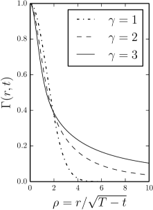
FIG. 1: The spatial degree function $k(r,t,T)$ and RP distribution function $\Gamma(r,t)$ for various exponents in 2 spatial dimensions. The models are characterized by $k_{\mathrm{max}}=k_{\mathrm{max}}(T-t)$ taken here to be linear: $k_{\mathrm{max}}(s)\propto s$.

III Analytical results

With this simple linear equation many network characteristics can be computed analytically. In what follows we will first prove an important relation between degrees and the RP distribution $\Gamma(x,t)$. Then we will outline the procedure which allows one to 1) derive the degree distribution when $\Gamma(x,t)$ is given, and more importantly 2) find $\Gamma(x,t)$ such that a desired degree distribution such as a power-law is obtained.

The degrees $k_{i}$ are defined as $k_{i}\equiv\sum_{j=1}^{N}A_{ij}$. Replacing the sum with an integral in the continuum limit and using $\int\mathrm{d}^{2}x_{j}G_{j}(x,t;x_{j},t_{0})=1$ for diffusion we obtain

$$k(x_{i},t_{0},T)= \lambda\int\int_{-\infty}^{T}\mathrm{d}t\,\mathrm{d}^{2}xG_{i}(x,t;x_{i},t_{0})\Gamma(x,t)$$ (8)

where $k(x_{i},t_{0},T)$ is the degree, measured at time $T,$ of an agent starting at position $x_{i}$ at time $t_{0}$. Applying $\mathscr{L}_{x_{i},t_{0}}^{\dagger}$ on both sides of (8) thus yields the first important result

$$\mathscr{L}_{x,t}^{\dagger}k(x,t,T)= \lambda\theta(T-t)\Gamma(x,t)$$ (9)

where $\theta(x)$ is the Heaviside step function. The significance of Eq. (9) is in that it relates the node degrees to the RP distribution. This allows us for instance to solve for the RP distribution required for an arbitrary degree distribution as we now proceed to do.

If $\Gamma$ is uniform over the space, each node will be overwhelmingly connected to those in its close vicinity, and the translational symmetry results in a sharply peaked degree distribution. Non-trivial degree distributions therefore arise only when this symmetry is broken. Let us now focus on rotationally symmetric RP distributions $\Gamma(r,t)$. With this symmetry the degree distribution $P(k)$ is an implicit function of $r,$ since $k$ is only a function of $r.$ For $P(k)$ monotonic (possibly with cutoffs near $k=0$ and $k_{\mathrm{max}}$), we have

$$P[k(r)]|\mathrm{d}k(r)| =|\mathrm{d}N(r)|$$ (10)

$$P[k(r)] =\left|\frac{\mathrm{d}N}{\mathrm{d}k}\right|=\frac{\mathrm{d}N}{\mathrm{d}r}\left|\frac{\mathrm{d}k}{\mathrm{d}r}\right|^{-1}$$ (11)

where $\mathrm{d}N(r)$ is the number of nodes in the annulus $[r,r+\mathrm{d}r].$ The absolute value is necessary since $\mathrm{d}k/\mathrm{d}r$ may be negative. This simple equation combined with (9) allows us to explicitly calculate the degree distribution given $\Gamma(x,t)$ or conversely, to solve for $\Gamma(x,t)$ given a desired degree distribution. As a simple example, with $t_{0}=0$ and a single rendezvous point activated at a single time, $\Gamma(r,t)=\delta(r)\delta(t-t_{e})$, equations (8) and (11) yield

$$P[k(r)]= 4\pi t_{e}\theta(T-t_{e})k^{-1}$$ (12)

which is a power law distribution $P(k)\propto k^{-\gamma}$ with exponent $\gamma=1$.

IV General power-law example

We will now derive the conditions for $\Gamma(r,t)$ for which the degree distribution becomes a power-law, possibly changing over time with an overall factor $p(T-t_{0})$ and with an upper cutoff

$$P(k;t_{0},T)=p(T-t_{0})k^{-\gamma},\quad k\in\left[1,k_{\mathrm{max}}\right].$$ (13)

The maximum degree $k_{\mathrm{max}}$ is chosen such that the expected number of nodes of degree $k_{\mathrm{max}}$ is one, i.e. $P(k_{\mathrm{max}})=1$. Therefore from (13)

$$k_{\mathrm{max}}\equiv p(T-t_{0})^{1/\gamma}.$$ (14)

Now, in order to solve for $\Gamma(r,t),$ we integrate (11) to find $k(r,t,T)$ and plug it in (9). We obtain

$$\Gamma(r,t) =\mathscr{L}_{\vec{r},t}^{\dagger}\left[\frac{\pi(\gamma-1)r^{2}+p(T-t)^{1/\gamma}}{p(T-t)}\right]^{\frac{1}{1-\gamma}}$$ (15)

For arbitrary $\gamma>1,$ and

$$\Gamma(r,t)=\mathscr{L}_{\vec{r},t}^{\dagger}\left\{p(T-t)\exp\left[\frac{\pi r^{2}}{p(T-t)}\right]\right\}$$ (16)

for $\gamma=1$.

The results for $\gamma=1,2,3$ and two different $p(t)$ are given in Fig. 1. Using these results, we can simulate the model by placing agents and RP’s on a finite area of the 2D space with appropriate distributions, and computing the $A_{ij}.$ To avoid boundary effects, the characteristic range of the random walkers $\sigma=\sqrt{4T}$ must be much smaller than the system size $L.$ For the continuum approximation to hold, $\sigma$ must be much larger than the inter-agent distance $L/\sqrt{N}.$ With proper normalization, $A_{ij}$ may be interpreted as the probability that the unweighted edge $(i,j)$ exists, and different realizations of the network can be constructed accordingly.

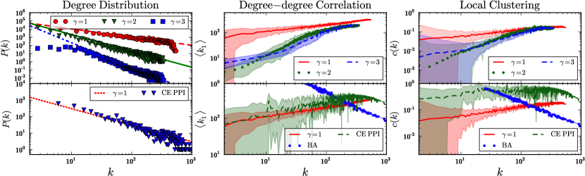
FIG. 2: Top left: degree distributions of graphs generated from our model for power-law distributions with $\gamma=1,2,3$. Lines represent $k^{-\gamma}$ for $\gamma=1,2,3$ (To separate data points for clarity a constant is multiplied into the y-axis of the 3 datasets). Top middle and top right show average degree of first neighbors, $\langle k_{1}\rangle$ vs degrees, and local clustering $c(k)$ for the 3 simulations, respectively. The curves are the means and the shaded area is one standard deviation above and below mean. Lower left: degree distribution of the C. elegans integrated protein interaction network danafarber . $P(k)\propto k^{-1}$ seems to match it well. Lower middle compares the degree assortativity of the C. elegans data (CE PPI) with our simulated $\gamma=1$ data, which almost perfectly reproduces the CE PPI statistics. The blue curve, BA, is a Barabasi-Albert network with $m=25$ (to produce comparable density) which exhibits a different behavior from our model and most parts of the CE PPI. Lower right compares the clustering of the three. Our model does seem to behave similar to the CE PPI, but it is no match for its extremely high clustering. Our global clustering for this $\gamma=1$ is $C=0.22$ whereas the CE PPI has $C=0.47$. Number of nodes and edges are $6.2\times 10^{3}$ and $1.8\times 10^{5}$ in CE PPI and $5.4\times 10^{3}$ and $2.1\times 10^{5}$ in $\gamma=1$.

IV.1 Higher moments: assortativity and clustering

The degree distribution is only one of many measures characterizing a graph. It is the distribution of the first moment $k_{i}=\sum_{j}A_{ij}$. The simplest among higher order measures of graph connectivity would be the degree-degree correlation, also known as degree assortativity, which compares the degree of the first neighbor of node $i$, $k_{i}^{1}$, to $k_{i}$ itself. The average first neighbor degree is

$$\langle k_{i}^{1}\rangle=\frac{1}{N}\sum_{j}A_{ij}k_{j}=\frac{1}{N}\sum_{j}[A^{2}]_{ij}$$

and is thus related to the square of the adjacency matrix.

The next higher order measure which is related to $A^{3}$ is the global clustering coefficient $C$ which measures the degree to which the graph is clustered newman2003structure

$$C\equiv\frac{3\times\#\mbox{ triangles}}{\#\mbox{ connected triplets}}.$$ (17)

which can be shown to be equal to $C=\mathrm{Tr}\left[A^{3}\right]/\sum_{ij}\left[A^{2}\right]_{ij}$. Clustering may also be measured at the vertex level using the local clustering $c_{i}$ newman2003structure defined as the number of triangles involving node $i$ divided by the total number of such triangles possible given the degree $k_{i}$

$$c_{i}\equiv\frac{2\times\mbox{\# triangles containing }i}{k_{i}(k_{i}-1)}.$$ (18)

By definition $c_{i}\leq 1$. Fig. 2 summarizes the results of simulations for scale-free distributions with $\gamma=1,2,3.$ For each case, one realization of the unweighted random graph ensemble is generated and the degree distributions $P(k)$, first neighbor degree-degree correlation $\langle k^{1}\rangle$, and local clustering $c(k)$ is shown. Interestingly, our model has a naturally high global clustering coefficient because agents close to the RP’s are all likely to connect and form close-knit subgraphs. Fig. 2 illustrates how our model compares to a particular real world network, namely the network of protein-protein interactions in the nematode C. elegans (CE PPI) from the integrated dataset of different types of interactions (incorporating WI8, literature curated, Microarray, Phenotype, Interolog, and Genetic interactions) danafarber , as well as a Barabasi-Albert (BA) network of similar size as the real data. The CE PPI network has a power-law degree distribution with power $P(k)\approx k^{-1}$. We therefore compare it with a $\gamma=1$ from our model. The PPI network has an average global clustering of $C=0.47$ versus our model’s $C=0.22$. The BA (with the same number of nodes as PPI and with $m=25$ to produce similar density) on the other hand, has $C=0.03$ and deviates significantly from the PPI data. In the first two moments, $P(k)$ and $\langle k^{1}\rangle$, our model matches the CE PPI almost perfectly. For clustering, our model exhibits a similar trend, but falls short in terms of magnitude.

V Discussion

We showed that networks with fat-tailed degree distributions and long range connections (scale-free networks are known to be “ultra small-world” PhysRevLett.90.058701 ) can arise from local interactions, if the translation symmetry is broken. The framework we introduced here uses the familiar tools of classical field theory. One of our main results is that given any (monotonic) degree distribution, we can analytically compute the RP distribution resulting in a network with that degree distribution.

While we demonstrated the derivations in the case of power-law distributions, other monotonic distributions can also be handled similarly. Furthermore, our model is generalizable to agent dynamics other than isotropic random walks, so long as the dynamics obeys a linear Fokker-Planck equation of the form $\mathscr{L}_{x,t}\phi(x,t)=J(x,t)$. Finally, the model can be solved in higher spatial dimensions as well, with similar results.

From the point of view of application, some real world networks, especially biological networks such as neuron firing correlation networks from fMRI measurements eguiluz2005scale and protein interaction networks PPI tend to have high global clustering coefficients ($C>20\%$). This is where many other scale-free network models such as Barabási-Albert (BA) fall short and there have been many attempts to remedy this holme2002growing ; volz2004random ; serrano2005tuning . One attractive feature of our model is that it has a naturally high global clustering. It also exhibits a degree-degree correlation pattern similar to biological data.

It must be stressed that this model was not originally intended as a model of protein-protein interactions. Nevertheless, it contains important elements that might constitute the ingredients for such a model. Accumulating mutations may be conceived of as a random walk inside some parameter space. A core set of existing genes can be represented by a distribution $\Gamma(r,t)$. Genotypic diversification mechanisms such as gene duplication may then correspond to branching processes, a simple example of which we presented in our model. These elements together with the partial empirical success of the model point to its potential utility as a starting point for modeling biological networks.

VI Acknowledgement

The authors wish to thank Shlomo Havlin for fruitful discussions. N.D. also wishes to thank Dina S. Ghiassian, Marc Santolini and the Barabási Lab for insightful discussions and for sharing their curated human interactome data. This material is based upon work supported in part by the National Science Foundation under grants No. 502019 and CMMI 1125290, and DTRA (Grant HDTRA-1-10-1-0014, Grant HDTRA-1-09-1-0035). N.D. also thanks Mary J. Hanf for valuable insights.

N.D. and N.D. contributed equally to this work.

References

- [1] Marc Barthélemy. Spatial networks. Physics Reports, 499(1–3):1–101, February 2011.
- [2] Reuven Cohen and Shlomo Havlin. Scale-free networks are ultrasmall. Phys. Rev. Lett., 90:058701, Feb 2003.
- [3] Harvard Medical School Dana Farber Cancer Institute. The worm interactome database, 2014.
- [4] S. N. Dorogovtsev and J. F. F. Mendes. Evolution of networks with aging of sites. Physical Review E, 62(2):1842–1845, August 2000.
- [5] Victor M Eguiluz, Dante R Chialvo, Guillermo A Cecchi, Marwan Baliki, and A Vania Apkarian. Scale-free brain functional networks. Physical review letters, 94(1):018102, 2005.
- [6] S Ghiassian, J Menche, and Albert-Laszlo Barabási. A disease module detection (diamond) algorithm derived from a systematic analysis of connectivity patterns of disease proteins in the human interactome, 2014.
- [7] Petter Holme and Beom Jun Kim. Growing scale-free networks with tunable clustering. Physical review E, 65(2):026107, 2002.
- [8] Austin L. Hughes. The Evolution of Functionally Novel Proteins after Gene Duplication. Proceedings of the Royal Society of London. Series B: Biological Sciences, 256(1346):119–124, May 1994.
- [9] J Sylvan Katz. Geographical proximity and scientific collaboration. Scientometrics, 31(1):31–43, 1994.
- [10] Konstantin Klemm and Víctor M. Eguíluz. Highly clustered scale-free networks. Physical Review E, 65(3):036123, February 2002.
- [11] P. L. Krapivsky and S. Redner. Organization of growing random networks. Physical Review E, 63(6):066123, May 2001.
- [12] Gautier Krings, Francesco Calabrese, Carlo Ratti, and Vincent D Blondel. Urban gravity: a model for inter-city telecommunication flows. Journal of Statistical Mechanics: Theory and Experiment, 2009(07):L07003, 2009.
- [13] Dmitri Krioukov, Fragkiskos Papadopoulos, Maksim Kitsak, Mariangeles Serrano, and Marian Boguna. Popularity versus similarity in growing networks. In APS Meeting Abstracts, volume 1, page 54009, 2012.
- [14] Dmitri Krioukov, Fragkiskos Papadopoulos, Maksim Kitsak, Amin Vahdat, and Marián Boguñá. Hyperbolic geometry of complex networks. Physical Review E, 82(3):036106, 2010.
- [15] Mark EJ Newman. The structure and function of complex networks. SIAM review, 45(2):167–256, 2003.
- [16] Susumu Ohno and others. Evolution by gene duplication. London: George Alien & Unwin Ltd. Berlin, Heidelberg and New York: Springer-Verlag., 1970.
- [17] Romualdo Pastor-Satorras, Eric Smith, and Ricard V. Solé. Evolving protein interaction networks through gene duplication. Journal of Theoretical biology, 222(2):199–210, 2003.
- [18] M Angeles Serrano and Marián Boguná. Tuning clustering in random networks with arbitrary degree distributions. Physical Review E, 72(3):036133, 2005.
- [19] Marc Vidal, Michael E. Cusick, and Albert-László Barabási. Interactome Networks and Human Disease. Cell, 144(6):986–998, March 2011.
- [20] Erik Volz. Random networks with tunable degree distribution and clustering. Physical Review E, 70(5):056115, 2004.
- [21] Duncan J Watts and Steven H Strogatz. Collective dynamics of ’small-world’ networks. Nature, 393:440–442, 1998.