Measurement of the Penetration Depth and Coherence Length of MgB₂ in All Directions Using Transmission Electron Microscopy

Abstract

We demonstrate that images of flux vortices in a superconductor taken with a transmission electron microscope can be used to measure the penetration depth and coherence length in all directions at the same temperature and magnetic field. This is particularly useful for MgB₂, where these quantities vary with the applied magnetic field and values are difficult to obtain at low field or in the $c$ direction. We obtained images of flux vortices from a MgB₂ single crystal cut in the $ac$ plane by focussed ion beam milling and tilted to $45^{\circ}$ with respect to the electron beam about the crystallographic $a$ axis. A new method was developed to simulate these images which accounted for vortices with a non-zero core in a thin, anisotropic superconductor and a simplex algorithm was used to make a quantitative comparison between the images and simulations to measure the penetration depths and coherence lengths. This gave penetration depths $\Lambda_{ab}=100\pm 35$ nm and $\Lambda_{c}=120\pm 15$ nm at 10.8 K in a field of 4.8 mT. The large error in $\Lambda_{ab}$ is a consequence of tilting the sample about $a$ and had it been tilted about $c$, the errors on $\Lambda_{ab}$ and $\Lambda_{c}$ would be reversed. Thus, obtaining the most precise values requires taking images of the flux lattice with the sample tilted in more than one direction. In a previous paper [J. C. Loudon et al., Phys. Rev. B 87, 144515, 2013], we obtained a more precise value for $\Lambda_{ab}$ using a sample cut in the $ab$ plane. Using this value gives $\Lambda_{ab}=107\pm 8$ nm, $\Lambda_{c}=120\pm 15$ nm, $\xi_{ab}=39\pm 11$ nm and $\xi_{c}=35\pm 10$ nm which agree well with measurements made using other techniques. The experiment required two days to conduct and does not require large-scale facilities. It was performed on a very small sample: $30\times 15$ $\upmu$m and 200 nm thick so this method could prove useful for superconductors where only small single crystals are available, as is the case for some iron-based superconductors.

I Introduction

Superconductors have zero electrical resistance and expel magnetic flux from their interiors (the Meissner effect). However, if a sufficiently high magnetic field is applied, flux penetrates by flowing along channels called flux vortices. Each vortex carries one quantum of magnetic flux, $\Phi_{0}=h/2e$ where $h$ is Planck’s constant and $e$ the electron charge. They consist of a core with a radius given by the coherence length, $\xi$, where the number of carriers (electrons or holes) contributing to superconductivity is suppressed. Electrical supercurrents circulate around the centre, diminishing over a radius given by the penetration depth, $\Lambda$. In a conventional superconductor, the coherence length is related to the energy required to excite a carrier out of the superconducting state, $\Delta$, and the velocity of the carriers at the Fermi energy, $v_{F}$, via $\xi=\hbar v_{F}/\pi\Delta$ and the penetration depth is related to the number density of carriers involved in superconductivity, $n_{S}$, and their effective mass, $m^{*}$, via $\Lambda=\sqrt{m^{*}/\mu_{0}n_{S}e^{2}}$ ($\mu_{0}$ is the permeability of free space).

In a type-I superconductor, the core exceeds the size over which the supercurrents persist and vortices attract one another as the area of normal (non-superconducting) material is minimised if the cores overlap. In a type-II superconductor, the supercurrents persist over a larger radius than the core and the Lorentz force causes vortices to repel one another so they form a hexagonal array in an isotropic superconductor. Introducing the Ginzburg-Landau parameter, $\kappa\equiv\Lambda/\xi$: a type-I superconductor has $\kappa<1/\sqrt{2}$ and type-II has $\kappa>1/\sqrt{2}$.

An anisotropic superconductor has different properties along different crystal axes, $a$, $b$ and $c$. Most are uniaxial so that $a$ and $b$ are equivalent. The anisotropy in the penetration depth is $\gamma_{\Lambda}\equiv\Lambda_{c}/\Lambda_{ab}$ and in the coherence length it is $\gamma_{\xi}\equiv\xi_{ab}/\xi_{c}$. In a 1-band superconductor, where there is one source of carriers contributing to superconductivity, the penetration depth and coherence length are independent of the applied magnetic field and their anisotropies are equal. One method to investigate the penetration depths and coherence lengths in both the $a$ and $c$ directions is to induce flux vortices with their axes normal to the $ac$ plane. The vortex then has an elliptical core surrounded by circulating currents as illustrated in Fig. 1(a).

Figure 1: (a) Flux vortex with its axis normal to the $ac$ plane. The core (shaded) is elliptical with dimensions $\xi_{ab}$ and $\xi_{c}$. Supercurrents ${\bf J}$ follow ellipses with the same aspect ratio, diminishing on lengthscales $\Lambda_{c}$ and $\Lambda_{ab}$. Streamlines of ${\bf J}$ are also contours of magnetic flux density ${\bf B}$. (b) Experimental arrangement for imaging flux vortices. The electron beam is deflected by the component of ${\bf B}$ normal to the beam so vortices appear as black-white features in an out-of-focus image. (c)–(f) Simulated images with defocus $\Delta f=7.15$ mm for a flux vortex in a 180 nm thick specimen in the orientation shown in (a) but tilted $45^{\circ}$ about $a$. Contrast values (see text) are shown below each image. (c) $\Lambda_{ab}=100$ nm, $\Lambda_{c}=120$ nm, $\xi_{V}=34$ nm, (d) $\Lambda_{ab}=100$ nm, $\Lambda_{c}=120$ nm, $\xi_{V}=1$ nm, (e) $\Lambda_{ab}=200$ nm, $\Lambda_{c}=120$ nm, $\xi_{V}=34$ nm, (f) $\Lambda_{ab}=100$ nm, $\Lambda_{c}=200$ nm, $\xi_{V}=34$ nm.

MgB₂ is a rare 2-band superconductor Nagamatsu et al. (2001) discovered in 2001 with a transition temperature $T_{c}=39$ K. It is uniaxial with a hexagonal crystal structure Nagamatsu et al. (2001) (space group 191: $P6/mmm$) composed of alternating layers of magnesium and boron with lattice parameters $a=b=3.086$ Å and $c=3.542$ Å. Two bands contribute to superconductivity: the $\sigma$-band associated with bonding from the boron $p_{xy}$ orbitals and the $\pi$-band associated with boron $p_{z}$ orbitals Choi et al. (2002). $\sigma$ carriers are confined to the $ab$ planes whereas the $\pi$ carriers are delocalised almost isotropically. At low magnetic fields, both $\sigma$ and $\pi$ bands contribute to superconductivity but as the field is increased, the $\pi$ contribution diminishes so that above 0.8 T (at 2 K), only the $\sigma$ band contributes Cubitt et al. (2003). This has the effect that the penetration depth and coherence length vary with field Cubitt et al. (2003).

In a previous paper Loudon et al. (2013), we showed that the penetration depth of MgB₂, $\Lambda_{ab}$, could be obtained in the low-field limit by making a quantitative comparison between images of flux vortices acquired using transmission electron microscopy and simulations. Here, we extend this method and show that the penetration depths $\Lambda_{ab}$ and $\Lambda_{c}$ and coherence lengths $\xi_{ab}$ and $\xi_{c}$ can be measured in a low field of 4.8 mT from a very small sample.

Focussed ion beam milling was used to cut a MgB₂ sample in the $ac$ plane of size $30\times 15$ $\upmu$m, thinned to 200 nm so that it was electron transparent (see section III). Flux vortices penetrate normal to the thin surfaces and the sample was tilted about its $a$ axis at $\alpha=45\pm 5^{\circ}$ to give a component of the B-field normal to the electron beam (Fig. 1(b)). The beam is deflected by the Lorentz force and flux vortices appear as black-white features in an out-of-focus image Harada et al. (1992). Such images are sensitive to the $B$-field throughout the thickness of the specimen, not just the stray field, and they can be acquired in real time Loudon (2015).

The effect on such images of changing the coherence length and penetration depth is shown in Fig. 1(c)–(f). These images were simulated by extending Beleggia’s method Beleggia et al. (2002) to model vortices with a non-zero core in a thin, anisotropic superconductor (see section II). We use Klemm and Clem’s Ginzburg-Landau model for the vortex core Clem (1980); Klemm and Clem (1980). In this model, the core has the same symmetry as the circulating currents so that $\xi_{ab}/\xi_{c}=\Lambda_{c}/\Lambda_{ab}$ and $\xi_{V}=\xi_{ab}^{1/3}\xi_{c}^{2/3}$ but any model for the magnetic structure of a flux vortex could be used with equal facility.

Fig. 1(c) shows a simulated image of a vortex with $\Lambda_{ab}=100$ nm, $\Lambda_{c}=120$ nm and $\xi_{V}=34$ nm. (d) shows that decreasing $\xi_{V}$ to 1 nm sharpens the image, increasing the contrast (the difference in the maximum and minimum intensities divided by their sum) from 10.5% to 14.8%. In (e), $\Lambda_{ab}$ is doubled which stretches the image in $c$ and reduces the contrast from 10.5% to 8.8%. (f) shows the images are most sensitive to $\Lambda_{c}$ so that when $\Lambda_{c}$ is increased to 200 nm, the image is stretched in $a$ and its contrast falls to 4.4%. This sensitivity of the images to changes in these parameters should allow the simultaneous measurement of the penetration depths and coherence lengths in all directions. In this paper we assess the accuracy of this new technique.

II Simulation of Flux Vortex Images

In this section, we present a model to calculate the magnetic fields generated by a flux vortex and from this simulate transmission electron micrographs. The model accounts not only for the B-field inside the superconductor but also for the spreading of the field lines near the superconductor surface and the field outside. It extends Beleggia’s method Beleggia and Pozzi (2001); Beleggia et al. (2002) to treat the case of a vortex in a thin, anisotropic superconducting slab and makes use of the work of Klemm and Clem Clem (1980); Klemm and Clem (1980); Clem et al. (1992) to account for a non-zero vortex core although it has the convenient feature that any model for the vortex core can be used with equal facility. Like all magnetic objects, flux vortices change only the phase and not the intensity of the electron beam and once the fields have been calculated, the phase shift can be found using the Aharanov-Bohm formula. Once the phase shift is known, any image can be simulated. Thus we first evaluate the magnetic vector potential, then use this to find the phase shift and from this simulate out-of-focus images of flux vortices.

II.1 Coordinate Systems

In order to visualise flux vortices using transmission electron microscopy, the specimen must be tilted by an angle $\alpha$ to provide a component of the B-field normal to the electron beam so that the electrons are deflected by the Lorentz force and show contrast in an out-of-focus image. Thus we follow Beleggia’s method Beleggia and Pozzi (2001); Beleggia et al. (2002) and introduce two coordinate systems: $X,Y,Z$ referring to the specimen with $X$ and $Y$ in the specimen plane and $Z$ normal to its surface and $x,y,z$ referring to the microscope with $z$ parallel to the electron beam as illustrated in Fig. 2. The specimen surfaces are at $Z=\pm d$ so its thickness is $t=2d$. We first evaluate the magnetic vector potential in terms of the specimen coordinates and use this to find the phase shift in the $xy$ plane which is equivalent to the plane in which images are recorded.

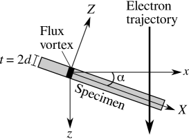
Figure 2: The relationship between the coordinates $X,Y,Z$, referring to the specimen and the microscope coordinates $x,y,z$. The $y$ and $Y$ axes are normal to the other two axes and point in the direction given by the right-hand rule. The axis of the vortex is parallel to $Z$ and the B-field enters the specimen at the bottom and exits at the top. The electron beam is parallel to $z$.

II.2 Magnetic Vector Potential

Here we evaluate the magnetic vector potential, ${\bf A}$, from a flux vortex passing through a thin superconducting slab with its axis directed along $Z$, normal to its surfaces. We use Beleggia’s Fourier-space method Beleggia and Pozzi (2001) throughout in which all the functions are Fourier transformed in $x$ and $y$ but not $z$ (or $X$ and $Y$ but not $Z$). This allows the Fourier transform of the vector potential and phase to be expressed by analytical but very lengthy expressions. These were evaluated symbolically using Matlab and only the final inverse transforms were performed numerically. For both coordinate systems, we use the transform convention that if $g(x,y,z)$ is a function in real-space, its Fourier transform $\widetilde{g}(k_{x},k_{y},z)$ is:

$$\widetilde{g}(k_{x},k_{y},z)=\int\limits_{-\infty}^{\infty}\int\limits_{-\infty}^{\infty}{g(x,y,z)e^{-i(k_{x}x+k_{y}y)}\,{\rm d}x{\rm d}y}$$ (1)

If the order parameter of the superconducting state is written in terms of its amplitude $f$ and phase $\theta$ as $\Psi=fe^{i\theta}$, the vector potential inside the superconductor is related to it by the 2nd Ginzburg-Landau equation Annett (2004); Ginzburg and Landau (1950):

$${\bf A}f^{2}+L\nabla\times(\nabla\times{\bf A})=\frac{\Phi_{0}}{2\pi}f^{2}\nabla\theta$$ (2)

where $L$ is penetration depth tensor. When $X,Y,Z$ are principal axes of the superconductor it has components:

$$L=\left(\begin{array}[]{ccc}\Lambda_{{}_{X}}^{2}&0&0\\ 0&\Lambda_{{}_{Y}}^{2}&0\\ 0&0&\Lambda_{{}_{Z}}^{2}\end{array}\right)$$ (3)

Following Clem Clem (1980), we look for a solution of the form

$${\bf A}={\bf A}_{\text{bulk}}+{\bf A}_{\text{surface}}$$ (4)

${\bf A}_{\text{bulk}}$ is the solution for a single vortex in an infinitely thick specimen and consequently has no $Z$-dependence. ${\bf A}_{\text{surface}}$ is the general solution with the correct boundary conditions but with the right-hand side of the Ginzburg-Landau equation set to zero.

Clem Clem (1975) solved for the bulk term in the isotropic case by using an order parameter for a single vortex of the form

$$\Psi=fe^{i\theta}=\frac{\rho}{\sqrt{\rho^{2}+\xi^{2}}}\,e^{-i\phi}$$ (5)

where $\rho$ is the radius from the axis of the vortex, $\phi$ is the azimuthal angle and $\xi$ is the coherence length. Klemm and Clem Klemm and Clem (1980); Clem et al. (1992) later extended this solution to the anisotropic case so that the order parameter becomes:

$$\Psi\!=\!\sqrt{\frac{X^{2}/\Lambda_{{}_{Y}}^{2}+Y^{2}/\Lambda_{{}_{X}}^{2}}{X^{2}/\Lambda_{{}_{Y}}^{2}+Y^{2}/\Lambda_{{}_{X}}^{2}+\xi^{2}/\Lambda^{2}}}\,e^{-i\arg(X/\Lambda_{{}_{Y}}+iY/\Lambda_{{}_{X}})}$$ (6)

where $\Lambda=(\Lambda_{{}_{X}}\Lambda_{{}_{Y}}\Lambda_{{}_{Z}})^{1/3}$. This gives the magnetic flux density as

$${\bf B}=\frac{\Phi_{0}}{2\pi\Lambda_{{}_{X}}\Lambda_{{}_{Y}}}\frac{K_{0}(R)}{(\xi/\Lambda)K_{1}(\xi/\Lambda)}\widehat{\bf Z}$$ (7)

where $R=\sqrt{(X/\Lambda_{{}_{Y}})^{2}+(Y/\Lambda_{{}_{X}})^{2}+(\xi/\Lambda)^{2}}$ and $K_{0}$ and $K_{1}$ are zero and first order modified Bessel functions.

Fourier transforming the flux density gives

$$\widetilde{\bf B}=\frac{\Phi_{0}K_{1}(Q\xi/\Lambda)}{QK_{1}(\xi/\Lambda)}\widehat{\bf Z}$$ (8)

where $Q=\sqrt{1+k_{{}_{X}}^{2}\Lambda_{{}_{Y}}^{2}+k_{{}_{Y}}^{2}\Lambda_{{}_{X}}^{2}}$. Since ${\bf B}=\nabla\times{\bf A}$, in Fourier space we have $\widetilde{\bf B}=(ik_{{}_{X}}\widetilde{A}_{Y}-ik_{{}_{Y}}\widetilde{A}_{X})\widehat{\bf Z}=i{\bf k}_{\perp}\times\widetilde{\bf A}$ where ${\bf k}_{\perp}=(k_{{}_{X}},k_{{}_{Y}},0)$. Imposing the additional requirement that ${\bf A}$ obey the London gauge $\nabla.{\bf A}=0$ so that $ik_{{}_{X}}\widetilde{A}_{X}+ik_{{}_{Y}}\widetilde{A}_{Y}=0$, the vector potential in Fourier space is

$$\widetilde{\bf A}_{\text{bulk}}=\frac{i\Phi_{0}K_{1}(Q\xi/\Lambda)}{k_{\perp}^{2}QK_{1}(\xi/\Lambda)}\left(\begin{array}[]{c}k_{{}_{Y}}\\ -k_{{}_{X}}\\ 0\end{array}\right)$$ (9)

We now find the surface term, ${\bf A}_{\rm surface}$. This is the general solution to the Ginzburg-Landau equation but where the right-hand side is set equal to zero. We use the approximation introduced by Clem Clem (1980) that the surface term should be only weakly influenced by the vortex core and so set $f^{2}=1$ in the search for a solution. The validity of this simplification was confirmed by Brandt Brandt (2005) who modelled the complete vortex and found that the core only expands by a few percent as it approaches the surface of the superconductor. The surface term is thus the solution to

$${\bf A}+L\nabla\times(\nabla\times{\bf A})=0$$ (10)

It should be noted that setting the right hand side of the Ginzburg-Landau equation (eqn. 2) to zero fixes the gauge of the vector potential and for an anisotropic superconductor, this is not the London gauge. Thus we cannot say $\nabla{\bf.A}=0$ nor make the convenient replacement $\nabla\times(\nabla\times{\bf A})=-\nabla^{2}{\bf A}$. Instead we must deal with the awkward cross-terms arising from the double curl.

Taking the Fourier transform of Eqn. 10 gives:

$$\widetilde{\bf A}+L(i\,{\bf k}_{\perp}+\widehat{\bf Z}\,\partial_{{}_{Z}})\times((i\,{\bf k}_{\perp}+\widehat{\bf Z}\,\partial_{{}_{Z}})\times\widetilde{\bf A})=0$$ (11)

We now postulate a solution of the form $\widetilde{\bf A}(k_{{}_{X}},k_{{}_{Y}},Z)={\bf a}(k_{{}_{X}},k_{{}_{Y}})e^{\beta Z}$ and the resulting equation can be written in matrix form as:

$$\left(\begin{array}[]{ccc}1+k_{{}_{Y}}^{2}\Lambda_{{}_{X}}^{2}-\Lambda_{{}_{X}}^{2}\beta^{2}&-k_{{}_{X}}k_{{}_{Y}}\Lambda_{{}_{X}}^{2}&ik_{{}_{X}}\Lambda_{{}_{X}}^{2}\beta\\ -k_{{}_{X}}k_{{}_{Y}}\Lambda_{{}_{Y}}^{2}&1+k_{{}_{X}}^{2}\Lambda_{{}_{Y}}^{2}-\Lambda_{{}_{Y}}^{2}\beta^{2}&ik_{{}_{Y}}\Lambda_{{}_{Y}}^{2}\beta\\ ik_{{}_{X}}\Lambda_{{}_{Z}}^{2}\beta&ik_{{}_{Y}}\Lambda_{{}_{Z}}^{2}\beta&1+\Lambda_{{}_{Z}}^{2}(k_{{}_{X}}^{2}+k_{{}_{Y}}^{2})\par\end{array}\right){\bf a}=\left(\begin{array}[]{c}0\\ 0\\ 0\end{array}\right)$$ (12)

The above equation gives non-zero solutions for the vector potential if the matrix cannot be inverted. To achieve this, values of $\beta$ must be found to make the determinant zero. At this point we introduce the symmetry of the problem otherwise the answers become very lengthy. For this experiment, the specimen was tilted about the $a$ axis and thus, $X\parallel c$, $Y\parallel a$ and $Z\parallel b$ so that $\Lambda_{{}_{X}}=\Lambda_{c}$ and $\Lambda_{{}_{Y}}=\Lambda_{ab}$ and $\Lambda_{{}_{Z}}=\Lambda_{ab}$. There are then four possible values of $\beta$:

$$\beta_{1,3}=\pm Q_{a}/\Lambda_{ab}$$ (13)

and

$$\beta_{2,4}=\pm Q/\Lambda_{c}$$ (14)

with corresponding eigenvectors

$${\bf a}_{1,3}=\left(\begin{array}[]{c}0\\ \pm iQ_{a}/(k_{{}_{Y}}\Lambda_{ab})\\ 1\end{array}\right)$$ (15)

and

$${\bf a}_{2,4}=\left(\begin{array}[]{c}\pm i\Lambda_{c}(1+k_{{}_{X}}^{2}\Lambda_{ab}^{2})/(\Lambda_{ab}^{2}k_{{}_{X}}Q)\\ \pm i\Lambda_{c}k_{{}_{Y}}/Q\\ 1\end{array}\right)$$ (16)

where $Q_{a}=\sqrt{1+(k_{{}_{X}}^{2}+k_{{}_{Y}}^{2})\Lambda_{ab}^{2}}$ and $Q=\sqrt{1+k_{{}_{X}}^{2}\Lambda_{ab}+k_{{}_{Y}}^{2}\Lambda_{c}}$. The complete vector potential inside the superconductor is then:

$$\widetilde{\bf A}_{\text{inside}}=\widetilde{\bf A}_{\text{bulk}}+\sum_{n=1}^{4}c_{n}{\bf a}_{n}e^{\beta_{n}z}$$ (17)

where $c_{1}$ – $c_{4}$ need to be determined by the boundary conditions.

This leaves the vector potential outside the superconductor to be determined. Maxwell’s third equation gives $\nabla\times{\bf B}=0$ as there are no electrical currents outside the superconductor so the vector potential obeys $\nabla\times(\nabla\times{\bf A})=0$. This time, the London gauge, $\nabla{\bf.A}=0$, may safely be invoked to give

$$\nabla^{2}{\bf A}_{\text{outside}}=0$$ (18)

or, in Fourier space:

$$-k_{\perp}^{2}\widetilde{\bf A}+\frac{\partial^{2}\widetilde{\bf A}}{\partial Z^{2}}=0$$ (19)

The solution to this is

$$\widetilde{\bf A}_{\text{top}}=\left(\begin{array}[]{c}c_{5}\\ c_{6}\\ i(c_{5}k_{{}_{X}}+c_{6}k_{{}_{Y}})/k_{\perp}\end{array}\right)e^{-k_{\perp}Z}$$ (20)

$$\widetilde{\bf A}_{\text{bottom}}=\left(\begin{array}[]{c}c_{7}\\ c_{8}\\ -i(c_{7}k_{{}_{X}}+c_{8}k_{{}_{Y}})/k_{\perp}\end{array}\right)e^{k_{\perp}Z}$$ (21)

where the $Z$-components are determined by the London gauge.

We can now simplify the equations as symmetry requires that $A_{{}_{X,Y}}(-Z)=A_{{}_{X,Y}}(Z)$ and $A_{{}_{Z}}(-Z)=-A_{{}_{Z}}(Z)$. This gives $c_{1}=-c_{3}$, $c_{2}=-c_{4}$, $c_{5}=c_{7}$ and $c_{6}=c_{8}$.

Summarising so far, the vector potential inside the superconductor is

$$\widetilde{\bf A}_{\text{inside}}=\widetilde{\bf A}_{\text{bulk}} + 2c_{1}\left(\begin{array}[]{c}a_{{}_{1,X}}\cosh(\beta_{1}Z)\\ a_{{}_{1,Y}}\cosh(\beta_{1}Z)\\ a_{{}_{1,Z}}\sinh(\beta_{1}Z)\end{array}\right)$$ (25)

$$+ 2c_{2}\left(\begin{array}[]{c}a_{{}_{2,X}}\cosh(\beta_{2}Z)\\ a_{{}_{2,Y}}\cosh(\beta_{2}Z)\\ a_{{}_{2,Z}}\sinh(\beta_{2}Z)\end{array}\right)$$ (29)

and above and below the superconductor, the vector potential is

$$\widetilde{\bf A}_{\text{above, below}}=\left(\begin{array}[]{c}c_{5}\\ c_{6}\\ \pm i(c_{5}k_{{}_{X}}+c_{6}k_{{}_{Y}})/k_{\perp}\end{array}\right)e^{\mp k_{\perp}Z}$$ (30)

To fix the values of $c_{1}$, $c_{2}$, $c_{5}$ and $c_{6}$, we invoke the following boundary conditions: (1) In order to calculate the phase shift from the vector potential, the $X$ and $Y$ components of the vector potential must change continuously across the boundary between the superconductor and vacuum at $Z=\pm d$. (2) The in-plane flux density $B_{\parallel}$ must be continuous across the boundaries at $Z=\pm d$ as there are no currents confined to the surface of the superconductor. There is also the requirement that the normal component of the flux density $B_{\perp}$ be continuous but this arises from Maxwell’s 3rd equation, $\nabla.{\bf B}=0$, and by using a vector potential, it is automatically satisfied.

Condition (1) that the in-plane vector potential is continuous at $Z=\pm d$ gives two equations (one for each component):

$$\widetilde{A}_{{}_{\text{bulk},X}}+2c_{1}a_{{}_{1,X}}\cosh(\beta_{1}d)+2c_{2}a_{{}_{2,X}}\cosh(\beta_{2}d)$$

$$=c_{5}e^{-k_{\perp}d}$$ (31)

$$\widetilde{A}_{{}_{\text{bulk},Y}}+2c_{1}a_{{}_{1,Y}}\cosh(\beta_{1}d)+2c_{2}a_{{}_{2,Y}}\cosh(\beta_{2}d)$$

$$=c_{6}e^{-k_{\perp}d}$$ (32)

Calculating the flux density via ${\bf B}=\nabla\times{\bf A}$ or, in Fourier space, $\widetilde{\bf B}=(i{\bf k}_{\perp}+\widehat{\bf z}\partial_{z})\times\widetilde{\bf A}$ and matching its in-plane components at the interface gives two more:

$$(-(k_{{}_{Y}}/k_{\perp})(c_{5}k_{{}_{X}}+c_{6}k_{{}_{Y}})+c_{6}k_{\perp})e^{-k_{\perp}d}=$$

$$2c_{1}D_{1}\sinh(\beta_{1}d)+2c_{2}D_{2}\sinh(\beta_{2}d)$$ (33)

$$(-c_{5}k_{\perp}+(k_{{}_{X}}/k_{\perp})(c_{5}k_{{}_{X}}+c_{6}k_{{}_{Y}}))e^{-k_{\perp}d}=$$

$$2c_{1}D_{3}\sinh(\beta_{1}d)+2c_{2}D_{4}\sinh(\beta_{2}d)$$ (34)

where $D_{1}=ik_{{}_{Y}}a_{{}_{1,Z}}-\beta_{1}a_{{}_{1,Y}}$, $D_{2}=ik_{{}_{Y}}a_{{}_{2,Z}}-\beta_{2}a_{{}_{2,Y}}$, $D_{3}=\beta_{1}a_{{}_{1,X}}-ik_{{}_{X}}a_{{}_{1,Z}}$ and $D_{4}=\beta_{2}a_{{}_{2,X}}-ik_{{}_{X}}a_{{}_{2,Z}}$

Writing these four equations in matrix form gives:

$$\left(\begin{array}[]{cccc}2D_{1}\sinh(\beta_{1}d)&2D_{2}\sinh(\beta_{2}d)&\frac{k_{{}_{X}}k_{{}_{Y}}}{k_{\perp}}e^{-k_{\perp}d}&\left(\frac{k_{{}_{Y}}^{2}}{k_{\perp}}-k_{\perp}\right)e^{-k_{\perp}d}\\ 2D_{3}\sinh(\beta_{1}d)&2D_{4}\sinh(\beta_{2}d)&-\left(\frac{k_{{}_{X}}^{2}}{k_{\perp}}-k_{\perp}\right)e^{-k_{\perp}d}&-\frac{k_{{}_{X}}k_{{}_{Y}}}{k_{\perp}}e^{-k_{\perp}d}\\ 2a_{1,x}\cosh(\beta_{1}d)&2a_{2,x}\cosh(\beta_{2}d)&-e^{-k_{\perp}d}&0\\ 2a_{1,y}\cosh(\beta_{1}d)&2a_{2,y}\cosh(\beta_{2}d)&0&-e^{-k_{\perp}d}\end{array}\right)\left(\begin{array}[]{c}c_{1}\\ c_{2}\\ c_{5}\\ c_{6}\end{array}\right)=\left(\begin{array}[]{c}0\\ 0\\ -\widetilde{A}_{{}_{\text{bulk},X}}\\ -\widetilde{A}_{{}_{\text{bulk},Y}}\end{array}\right)$$ (35)

The coefficients $c_{1}$, $c_{2}$, $c_{5}$, $c_{6}$ can then be found by inverting the matrix and then, after substituting the answers into Eqns. 25 and 30, the vector potential is fully determined. It should be noted that although we use Klemm and Clem’s solution for ${\bf A}_{\text{bulk}}$, Eqn. 35 shows that our method has the convenient feature that any model for ${\bf A}_{\text{bulk}}$ could be used with equal facility.

II.3 Phase Shift

The magnetic contribution to the phase shift suffered by the electron beam after passing through a specimen is related to the vector potential via the Aharanov-Bohm expression:

$$\phi(x,y)=-\frac{2\pi e}{h}\int_{-\infty}^{\infty}{\bf A}(x,y,z){\bf.}{\rm d}{\bf l}$$ (36)

where ${\rm d}{\bf l}$ is an increment along the trajectory of the electrons shown in Fig. 3. If unit vectors in $x$, $y$ and $z$ of the microscope coordinate system are denoted ${\bf i}$, ${\bf j}$ and ${\bf k}$ and those in $X$, $Y$ and $Z$ of the specimen coordinate system are denoted ${\bf I}$, ${\bf J}$ and ${\bf K}$, the two sets of unit vectors are related via:

$${\bf I} = {\bf i}\cos\alpha+{\bf k}\sin\alpha$$ (37)

$${\bf J} = -{\bf j}$$ (38)

$${\bf K} = {\bf i}\sin\alpha-{\bf k}\cos\alpha$$ (39)

If the electron passes through the specimen at position $(X,Y,0)$ and if for the preceding part of its journey, we label the height above the specimen in the $Z$ direction $w$ (see Fig. 3), its position at any point in its trajectory is given by

$${\bf l}=(X-w\tan\alpha){\bf I}+Y{\bf J}+w{\bf K}$$ (40)

By differentiating the above equation, an increment in its trajectory ${\rm d}{\bf l}$ can be related to an increment in $w$ via:

$${\rm d}{\bf l}=(-\tan\alpha\,{\bf I}+{\bf K}){\rm d}w$$ (41)

Figure 3: The relationship between the coordinates $X,Y,Z$, referring to the specimen (shown by the grey rectangle) and the microscope coordinates $x,y,z$.

The phase shift written in terms of the specimen coordinates is thus:

$$\phi(X,Y)=-\frac{2\pi e}{h}\times$$

$$\int_{-\infty}^{\infty}{\bf A}(X-w\tan\alpha,Y,w).\left(\begin{array}[]{c}-\tan\alpha\\ 0\\ 1\end{array}\right)\,{\rm d}w$$ (45)

In the previous section the vector potential was calculated in Fourier space. This is related to the vector potential in real-space via the inverse Fourier transform:

$${\bf A}( X ,Y,Z)=$$ (46)

$$\frac{1}{4\pi^{2}}\int\limits_{-\infty}^{\infty}\int\limits_{-\infty}^{\infty}{\widetilde{\bf A}(k_{{}_{X}},k_{{}_{Y}},Z)e^{i{\bf k}_{\perp}.{\bf R}}\,{\rm d}k_{{}_{X}}\,{\rm d}k_{{}_{Y}}}$$

where ${\bf R}=(X,Y,Z)$. Thus it follows that

$${\bf A}(X-w\tan\alpha,Y,Z)=$$

$$\frac{1}{4\pi^{2}}\iint\widetilde{\bf A}(k_{{}_{X}},k_{{}_{Y}},Z)e^{i{\bf k}_{\perp}.{\bf R}}e^{-ik_{{}_{X}}w\tan\alpha}\,{\rm d}k_{{}_{X}}\,{\rm d}k_{{}_{Y}}$$ (47)

So the phase shift is

$$\phi(X,Y)=-\frac{2\pi e}{h}\int_{-\infty}^{\infty}\left(\frac{1}{4\pi^{2}}\iint\widetilde{\bf A}(k_{{}_{X}},k_{{}_{Y}},w)e^{i{\bf k}_{\perp}.{\bf R}}e^{-ik_{{}_{X}}w\tan\alpha}\,{\rm d}k_{{}_{X}}\,{\rm d}k_{{}_{Y}}\right).\left(\begin{array}[]{c}-\tan\alpha\\ 0\\ 1\end{array}\right)\,{\rm d}w$$ (48)

It can be seen from Fig. 3 that if an electron passes through a point $(X,Y,0)$ on the specimen, it passed through a point $(x,y,0)$ in the $xy$ plane where $x=X\cos\alpha$ and $y=-Y$. The phase shift in the $xy$-plane (which is equivalent to the plane in which the image is taken) is now found by making this substitution.

$$\phi(x,y)=-\frac{2\pi e}{h}\int_{-\infty}^{\infty}\left(\frac{1}{4\pi^{2}}\iint\widetilde{\bf A}(k_{{}_{X}},k_{{}_{Y}},w)e^{ik_{{}_{X}}x/\cos\alpha}e^{-ik_{{}_{Y}}y}e^{-ik_{{}_{X}}w\tan\alpha}\,{\rm d}k_{{}_{X}}\,{\rm d}k_{{}_{Y}}\right).\left(\begin{array}[]{c}-\tan\alpha\\ 0\\ 1\end{array}\right)\,{\rm d}w$$ (49)

Now let $k_{x}=k_{{}_{X}}/\cos\alpha$ and $k_{y}=-k_{{}_{Y}}$:

$$\phi(x,y)=\frac{2\pi e}{h}\int_{-\infty}^{\infty}\left(\frac{1}{4\pi^{2}}\iint\widetilde{\bf A}(k_{x}\cos\alpha,-k_{y},w)e^{ik_{x}x}e^{ik_{y}y}e^{-ik_{x}w\sin\alpha}\cos\alpha\,{\rm d}k_{x}\,{\rm d}k_{y}\right).\left(\begin{array}[]{c}-\tan\alpha\\ 0\\ 1\end{array}\right)\,{\rm d}w$$ (50)

Changing the order of integration gives:

$$\phi(x,y)=\frac{2\pi e\cos\alpha}{h}\frac{1}{4\pi^{2}}\iint e^{i{\bf k_{\perp}.r}}\left(\int_{-\infty}^{\infty}\widetilde{\bf A}(k_{x}\cos\alpha,-k_{y},w)e^{-ik_{x}w\sin\alpha}\,{\rm d}w\right)\,{\rm d}k_{x}\,{\rm d}k_{y}.\left(\begin{array}[]{c}-\tan\alpha\\ 0\\ 1\end{array}\right)$$ (51)

or representing an inverse Fourier transform as IFT and using the flux quantum $\Phi_{0}$ we have:

$$\phi(x,y)={\rm IFT}\left[\frac{\pi}{\Phi_{0}}\left(\begin{array}[]{c}-\sin\alpha\\ 0\\ \cos\alpha\end{array}\right).\,\int_{-\infty}^{\infty}\widetilde{\bf A}(k_{x}\cos\alpha,-k_{y},w)e^{-ik_{x}w\sin\alpha}\,{\rm d}w\right]$$ (52)

The integral over $w$ is straightforward as it only involves exponential functions but it is very lengthy so it and the scalar product were performed symbolically using Matlab. Only the final inverse Fourier transform which gives the phase was evaluated numerically.

A method to check the correctness of the solution is to plot the phase shift as a contour map for $\alpha=90^{\circ}$. This gives the B-field projected through the thickness of the specimen and is shown in Fig. 4. It can be seen that the correct boundary conditions are fulfilled: the field lines spread as they approach the specimen surface from the interior and outside the specimen they are straight so that the field resembles that from a monopole if viewed far from the vortex. The figure shows that the effect of increasing the coherence length $\xi_{V}$ is to make the field less intense near the centre of the vortex as expected.

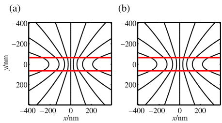
Figure 4: Contours of the phase-shift spaced by 0.2 rad illustrating the projected B-field from a flux vortex with $\Lambda_{ab}=100$ nm and $\Lambda_{c}=120$ nm and (a) $\xi_{V}=1$ nm and (b) $\xi_{V}=36$ nm. The red lines indicate the surfaces of the specimen which is 128 nm thick. The $a$-axis is parallel to $x$ with $c$ pointing into the page.

II.4 Image Simulation

Once the phase shift $\phi(x,y)$ has been calculated, the wavefunction of the electron beam is $\psi_{0}(x,y)=e^{i\phi}$ and the intensity of the in-focus bright-field image is $I_{0}(x,y)=|\psi_{0}(x,y)|^{2}$. It is immediately clear that this gives 1 and an in-focus image is therefore featureless. In order to visualise flux vortices, out-of-focus images must be taken. Taking an out-of-focus image is equivalent to propagating the wavefunction through free space by a distance $\Delta f$, known as the defocus. This is done via the Fresnel-Kirchoff integral Beleggia et al. (2002) so that the defocussed wavefunction $\psi_{\Delta f}(x,y)$ is related to the in-focus wavefunction via:

$$\psi_{\Delta f}(x,y)=$$

$$\frac{1}{\lambda\Delta f}\iint \psi_{0}(x^{\prime},y^{\prime}) e^{\frac{i\pi}{\lambda\Delta f}((x-x^{\prime})^{2}+(y-y^{\prime})^{2})}\,{\rm d}x^{\prime}{\rm d}y^{\prime}$$ (53)

where $\lambda$ is the electron wavelength. This is a convolution and so is more conveniently evaluated as a multiplication in Fourier space via:

$$\widetilde{\psi}_{\Delta f}=\widetilde{\psi}_{0}e^{-i\lambda\Delta fk^{2}/4\pi}$$ (54)

After inverse transforming, the intensity in the out-of-focus image is given by $I_{\Delta f}=|\psi_{\Delta f}|^{2}$.

III Experimental Method

MgB₂ single crystals were synthesised by the peritectic decomposition of MgNB₉ and their quality and bulk properties have been well characterised by a variety of experimental techniques Karpinski et al. (2003, 2007); Zhigadlo et al. (2010). The samples were prepared for electron microscopy at the Technical University of Denmark (DTU) using a Helios Nanolab focussed ion beam microscope (FIB). This is a dual-beam instrument in which a beam of gallium ions is used to mill the specimen whilst secondary electrons emitted by the specimen are used to produce an image, however an electron beam can also be used to illuminate the specimen in order to take images without damaging the specimen.

The MgB₂ single crystals were about $1\times 1$ mm in the $ab$ plane and about 100 $\upmu$m thick in the $c$-direction. The in-situ lift-out technique was used to prepare the sample for electron microscopy. First, the FIB was used to deposit a 3 $\upmu$m thick, $30\times 5$ $\upmu$m rectangle of platinum onto the $ab$ surface to protect the sample beneath from ion damage. Trenches were then milled to a depth of $20$ $\upmu$m in the $c$ direction around this to produce a slab standing in the centre of a crater. The top surface of the sample was smooth and this avoided the creation of the longitudinal thickness undulations reported in our last paper Loudon et al. (2013).

A movable needle known as a micromanipulator was attached to the slab using platinum deposition and the slab was cut away from the rest of the specimen and extracted on the end of the micromanipulator. A sample can be tilted only to $25^{\circ}$ in the electron microscope so to achieve a higher tilt angle, the FIB was used to cut a slot at $45^{\circ}$ to the plane of an ‘Omniprobe’ grid. Further platinum deposition was used to attach the sample to this slot and the micromanipulator was then cut away, leaving the sample attached to the grid and tilted about its $a$ axis by $45^{\circ}$ with respect to the plane of the grid. The sample was then thinned to approximately 200 nm so that it was electron-transparent using a 30 kV Ga ion beam. Finally, the specimen surfaces were polished by a low-energy (2kV) Ga ion beam to minimise the damage layer caused by FIB milling.

Electron microscopy was undertaken at DTU using an FEI Titan 80-300ST transmission electron microscope operated at 300 kV equipped with a Gatan imaging filter to record images. Under normal operating conditions, the main objective lens of the microscope applies a 2 T field to the specimen so to avoid this, the microscope was operated in low-magnification mode with the main objective lens set to a low value and the image was focussed with the diffraction lens. Prior to imaging vortices, electron diffraction was used to make a fine adjustment of a few degrees so that the tilt was purely about the $a$ axis. Adjusting the sample so that it is tilted purely about $a$ can be performed to better than $0.5^{\circ}$ but this may alter the overall tilt angle and we judge that the tilt angle was $\alpha=45\pm 5^{\circ}$.

The simulations were based on elastic electron scattering so experimental images were energy filtered so that only electrons which had lost 0–10 eV on passing through the specimen contributed and an aperture was used so that only the 000 beam and the low-angle scattering from the vortices contributed to the image and the other crystallographic beams were excluded. The sample was cooled using a Gatan liquid-helium cooled ‘IKHCHDT3010-Special’ tilt-rotate holder which has a base temperature of 10 K.

The defocus and magnification were calibrated by acquiring images with the same lens settings as the original images from Agar Scientific’s ‘S106’ calibration specimen which consists of lines spaced by 463 nm ruled on an amorphous film. The defocus was found by taking digital Fourier transforms of the images acquired from the calibration specimen and measuring the radii of the dark rings which result from the contrast transfer function Williams and Carter (1996).

A thickness map of the specimen was created by dividing an unfiltered image by an energy-filtered image and taking the natural logarithm Egerton (2009) which gives the thickness parallel to the electron beam, $l$, as a multiple of the inelastic mean free path, $\lambda_{i}$. To determine $\lambda_{i}$, an electron hologram was taken at room temperature at an edge of the specimen which gives a phase shift proportional to the thickness, $\phi=C_{E}V_{0}l$. $C_{E}$ is a constant which depends only on the microscope voltage and has the value $6.523\times 10^{6}$ m^-1V^-1 at 300 kV. $V_{0}$, the mean inner potential, was calculated as $V_{0}=17.71$ V from theoretical scattering factors given in ref. Rez et al., 1994, giving $\lambda_{i}=244\pm 5$ nm and the thickness, $l$, varied from 200–290 nm across the field of view of Fig. 5. Ideally the thickness of the whole specimen would have been determined by electron holography but the field of view of the interference region was not sufficiently large.

A simplex algorithm Press et al. (1992) was used to minimise the reduced $\chi^{2}$ value between the experimental images and simulations by fitting the vortex positions and the in-plane rotation angle of the vortices as well as $\Lambda_{ab}$, $\Lambda_{c}$ and $\xi_{V}$. The reduced $\chi^{2}$ value is defined as $\chi^{2}\equiv(1/N)\sum_{j=1}^{N}(I^{\rm experiment}_{j}-I^{\rm simulation}_{j})^{2}/\sigma_{j}^{2}$ where $N$ is the number of pixels used in the fit, $I_{j}$ is the intensity of pixel $j$ in the image and $\sigma_{j}$ is the noise associated with pixel $j$. We used $\sigma_{j}^{2}=cI^{\rm simulation}_{j}$ having previously taken a series of images of the vacuum with different electron intensities. A graph of the standard deviation versus the average intensity showed the noise was Shot noise (so that the square of the noise was proportional to the image intensity) and gave the proportionality constant $c$ relating the counts recorded on the detector to the number of electrons received. Unlike our previous publication where separate fits were made for each vortex Loudon et al. (2012), here all the vortex images were fit simultaneously with a single value of $\Lambda_{ab}$, $\Lambda_{c}$ and $\xi_{V}$ using the model described in section II.

IV Results

Fig. 5(a)–(f) show an experimental defocus series acquired at 10.8 K (the base temperature of our cooling stage) in a field of 4.8 mT. $68$ images of vortices which were least affected by bend contrast were fit and with a single value of $\Lambda_{ab}$, $\Lambda_{c}$ and $\xi_{V}$ along with the position of each vortex and its in-plane rotation angle using a simplex algorithm Press et al. (1992) to minimise the reduced $\chi^{2}$ value. The specimen thickness and tilt angle were fixed at their calibrated values.

Fig. 5(g) shows the average of these images at each defocus level and (h) shows the average of the fitted simulations. To demonstrate that the fit is good, (i) shows the difference between images and simulations and (j) compares linescans taken across the vortex images.

Figure 5: (a)–(f) Defocus series showing flux vortices in MgB₂ at 10.8 K in a field of 4.8 mT with defoci: (a) $\Delta f=-21.4$, (b) $-14.3$, (c) $-7.15$, (d) $7.15$, (e) $14.3$ and (f) $21.4$ mm. (g) Average vortex images at each defocus level. (h) Average simulated images. (i) Difference images between experiment and simulation. (j) Linescans across the images from the region shown by the red box in (h). Black lines show experimental data and red lines the fit.

$\Lambda_{ab}$, $\Lambda_{c}$ and $\xi_{V}$ were then altered in turn and the errorbar on each judged by the point at which the difference images displayed a discernibly worse fit as shown in Fig. 6(a)–(d). This corresponded to an increase in the reduced $\chi^{2}$ of 0.009 and the variation of $\chi^{2}$ as each parameter is varies is shown in Fig. 6(e). This yielded $\Lambda_{ab}=107\pm 33$ nm, $\Lambda_{c}=134\pm 6$ nm and $\xi_{V}=31\pm 9$ nm. The images are much more sensitive to the value of $\Lambda_{c}$ than to $\Lambda_{ab}$ as a consequence of mounting the sample tilted about the $a$ axis: had it been tilted about $c$, the errors on $\Lambda_{ab}$ and $\Lambda_{c}$ would be reversed. In a previous paper Loudon et al. (2013), we obtained the more precise value of $\Lambda_{ab}=107\pm 8$ nm using a sample cut in the $ab$ plane.

To check for amorphous ‘dead-layers’ of non-superconducting material on the sample surfaces caused by ion thinning, the thickness of the crystalline component of the sample was measured using the convergent beam diffraction technique described in ref. Williams and Carter, 1996. This showed no difference between the total and crystalline thicknesses to within the experimental error of $\pm 10$ nm. Reducing the calibrated thickness values by 50 nm to account for the largest conceivable dead-layer reduced $\Lambda_{ab}$ by 13 nm, reduced $\Lambda_{c}$ by 27 nm and increased $\xi_{V}$ by 10 nm without altering the quality of the fit. Taking this into account gives: $\Lambda_{ab}=100\pm 35$ nm, $\Lambda_{c}=120\pm 15$ nm and $\xi_{V}=36\pm 10$ nm. The anisotropy ratio in the penetration depth is then $\gamma_{\Lambda}=1.2\pm 0.4$ and the coherence lengths are $\xi_{ab}=\gamma^{2/3}\xi_{V}=41\pm 13$ nm and $\xi_{c}=\gamma^{-1/3}\xi_{V}=34\pm 10$ nm. Alternatively, using the more precise value of $\Lambda_{ab}=107\pm 8$ nm and $\Lambda_{c}=120\pm 15$ nm gives $\gamma_{\Lambda}=1.12\pm 0.16$, $\xi_{ab}=39\pm 11$ nm and $\xi_{c}=35\pm 10$ nm.

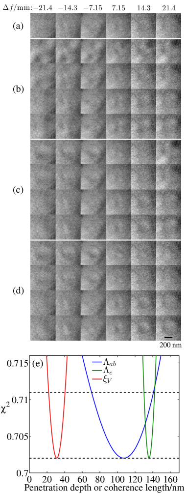
Figure 6: Difference images between the average defocus series and simulated images as each parameter is varied. (a) Difference images for the best-fit values of the parameters. (b) Difference images when $\Lambda_{ab}$ is varied: the top row shows difference images when $\Lambda_{ab}$ is set at two errorbars below the best-fit value. The next row is for $\Lambda_{ab}$ set one errorbar below. The next two rows are for $\Lambda_{ab}$ increased one and two errorbars above the best-fit value respectively. (c) A similar series showing the effect of changing $\Lambda_{c}$. (d) Series showing the effect of changing $\xi_{V}$. (e) Reduced $\chi^{2}$ values as $\Lambda_{ab}$, $\Lambda_{c}$ and $\xi_{V}$ are adjusted. Acceptable values of $\chi^{2}$ lie between the dashed lines.

V Discussion

We now compare the values obtained here with those found using other techniques. These show that the conditions used (4.8 mT and 10.8 K) were in the low field limit ($<100$ mT as established by neutron diffraction) but not quite in the low temperature limit ($<5$ K from radio-frequency measurements).

In 2005, Fletcher et al. Fletcher et al. (2005) performed radio-frequency measurements which gave the change in the low-field penetration depth with temperature but not absolute values. At 10.8 K, $\Lambda_{ab}$ increased by $12\pm 1$ nm and $\Lambda_{c}$ increased by $18\pm 4$ nm with respect to their low temperature values. Subtracting these from our most precise measurements of the penetration depths gives $\Lambda_{ab}=95\pm\ 8$ nm and $\Lambda_{c}=102\pm 15$ nm and the anisotropy as $\gamma=1.07\pm 0.18$ in the low field and low temperature limit.

The most reliable measurement of the absolute value of the penetration depth is likely to be from neutron diffraction and in 2003 Cubitt et al. Cubitt et al. (2003) found that at 2 K, the extrapolated low field ($<100$ mT) value was $\Lambda_{ab}=82\pm 2$ nm which is close to our value.

As samples grow as thin plates in the $ab$ plane, Cubitt et al. did not have direct access to $\Lambda_{c}$ and so acquired diffraction patterns with vortices tilted at $45^{\circ}$ with respect to the $c$-axis. It was uncertain whether the formula used to calculate the anisotropy was valid for a 2-band superconductor Cubitt et al. (2003) but data acquired at 2 K between 0.2–0.5 T indicated that $\gamma_{\Lambda}$ varied with field and its extrapolated value at low field was $\gamma_{\Lambda}=1.1\pm 0.3$. In 2006, Pal et al. Pal et al. (2006) used a different neutron diffraction technique to give $\gamma_{\Lambda}=1.1\pm 0.1$ at 4.9 K. Combining this with the neutron value for $\Lambda_{ab}$ gives $\Lambda_{c}=90\pm 8$ nm which agrees with our value of $\Lambda_{c}=102\pm 15$ nm. The anisotropy we obtain is close to the value of 1.01 calculated from first-principles by Golubov et al. Golubov et al. (2002) in the clean limit but in common with Fletcher et al. Fletcher et al. (2005), we find penetration depths approximately twice as large as predicted.

Cubitt et al. interpreted their data assuming that the coherence length did not vary with field. If it did, the value they obtained, $\xi_{ab}=8\pm 1$ nm, would apply only at high field ($>0.8$ T). This is close to the value of 10 nm found from the upper critical field Eskildsen et al. (2003).

Eskildsen et al. Eskildsen et al. (2002) measured the coherence length in 2002 using scanning tunnelling microscopy (STM) to measure the width of vortex cores, scanning the $ab$ plane with tunnelling in $c$. As the $\sigma$ carriers are confined to the $ab$-planes, the tunnelling current came almost exclusively from the $\pi$ band giving $\xi_{\pi}=38.8\pm 0.7$ nm at 0.32 K in a field of 50 mT (after adjusting for their slightly different model for the core). This agrees with our value of $\xi_{c}=35\pm 10$ nm at 10.8 K and 4.8 mT and supports this larger value at low field.

VI Summary and Conclusions

We have described a new method to measure the penetration depth and coherence length of a superconductor in all directions at low applied magnetic field using transmission electron microscopy. The measurement does not need large-scale facilities and required one day to thin and mount the sample and another day to take the images required. The experiment was performed on a very small sample: $30\times 15$ $\upmu$m and 200 nm thick so this method could prove useful for superconductors where only very small single crystals are available, as is the case for some iron-based superconductors. It is also useful if the penetration depth and coherence length vary with field, as is the case for MgB₂, as the measurement is made at very low fields which can be difficult to access using other techniques.

For a sample of MgB₂ cut in the $ac$ plane and tilted to $45\pm 5^{\circ}$ about the $a$-axis, we obtained $\Lambda_{ab}=100\pm 35$ nm, $\Lambda_{c}=120\pm 15$ nm at 10.8 K in a field of 4.8 mT. The large error in $\Lambda_{ab}$ is a consequence of tilting the sample about the crystallographic $a$ axis. Had it been tilted about $c$ instead, the errors on $\Lambda_{ab}$ and $\Lambda_{c}$ would be reversed. We obtained a more precise value of $\Lambda_{ab}=107\pm 8$ nm at 10.8 K in our previous paper Loudon et al. (2013) in which the sample was cut in the $ab$ plane. Using this value gives $\Lambda_{ab}=107\pm 8$ nm, $\Lambda_{c}=120\pm 15$ nm, $\xi_{ab}=39\pm 11$ nm and $\xi_{c}=35\pm 10$ nm which agree well with measurements made using other techniques discussed in section V.

Obtaining the most precise values for the penetration depths and coherence lengths in all directions using this technique requires taking images of the vortex lattice with the sample tilted in more than one direction. It might be thought that the sample could be mounted in the plane of the support grid and tilted with the microscope goniometer, first about $a$ and then about $c$. However, the design of conventional liquid helium cooled holders does not allow tilting to an angle higher than $\alpha=25^{\circ}$, so the sample was instead mounted to the support grid at $45\pm 5^{\circ}$ to give sufficient contrast in the image. Thus, to investigate a new superconductor and obtain the most accurate measurement of the penetration depth and coherence length in all directions, it would be best to cut two samples and mount both to the grid, one tilted about $a$ and the other tilted about $c$.

We used the Ginzburg-Landau model for the magnetic structure of flux vortices but as MgB₂ is a two-band superconductor, the vortices may well have a more complex structure as described in ref. Babaev and Carlström, 2010. We obtained good fits to the vortex images and there was no indication of a more complex structure within the accuracy of the technique but our simulation scheme would allow any model for the vortex structure to be used for image simulations provided that the magnetic vector potential for a vortex in an infinitely thick superconductor is known.