Static critical behavior of the $q-$states Potts model: High-resolution entropic study

Abstract

Here we report a precise computer simulation study of the static critical properties of the two-dimensional $q$-states Potts model using very accurate data obtained from a modified Wang-Landau (WL) scheme proposed by Caparica and Cunha-Netto [Phys. Rev. E 85, 046702 (2012)]. This algorithm is an extension of the conventional WL sampling, but the authors changed the criterion to update the density of states during the random walk and established a new procedure to windup the simulation run. These few changes have allowed a more precise microcanonical averaging which is essential to a reliable finite-size scaling analysis. In this work we used this new technique to determine the static critical exponents $\beta$, $\gamma$, and $\nu$, in an unambiguous fashion. The static critical exponents were determined as $\beta=0.10811(77)$, $\gamma=1.4459(31)$, and $\nu=0.8197(17)$, for the $q=3$ case, and $\beta=0.0877(37)$, $\gamma=1.3161(69)$, and $\nu=0.7076(10)$, for the $q=4$ Potts model. A comparison of the present results with conjectured values and with those obtained from other well established approaches strengthens this new way of performing WL simulations.

I Introduction

Monte Carlo (MC) simulations are ubiquitous in the field of statistical mechanics, especially for the study of phase transitions and critical phenomena Binder2000 ; krauth2006 . Since the historical work of Metropolis et al Metropolis1953 , the most outstanding task in this context is the pursuit of new and more efficient algorithms to overcome long time scale problems. Since there are few problems in the field of interacting systems for which one can find an exact solution, MC simulations became an indispensable tool. This is due to the massively increasing in computational power and further due to the development of more efficient algorithms. More recently, such development focused on the extended ensemble method, where one uses an ensemble different from the ordinary canonical with a fixed temperature, as in the original Metropolis algorithm. To name a fill examples we have the multicanonical method BergNeuhaus1992 , and the exchange Monte Carlo method (parallel tempering) Nemoto1996 . Particularly, during the last two decades, a multicanonical MC algorithm known as Wang-Landau sampling WangLandau2001 , has been at the forefront of interest Dayaletal2004 and has proven to be a very powerful numerical procedure for the study of phase transitions and critical phenomena Landau2004 ; Nogawa2001 ; blume .

The original idea of the WL algorithm is to measure an a priori unknown density of states of a given system iteratively by performing a random walk in energy space and sampling configurations with probability proportional to the reciprocal of the density of states, resulting in a “flat” histogram. Despite being a well-established numerical procedure, it is clear that some improvements on the algorithm are indeed necessary to overcome some limitations during the simulation run. The method itself was subject to several studies and various improvements to it have been proposed kawashima ; ZhouBhatt2005 ; belardinelli . By its turn, the MC algorithm used in this work is an extension of the conventional WL where some few changes produce more reliable and precise results.

Considering the aforementioned comments, the purpose of this paper is twofold. First, to present a numerically simple and accurate procedure to halting a regular WL simulation run. This is accomplished with a method proposed in Refs. caparica ; caparica3 . Second, to apply this technique to the square two-dimensional $q$-state Potts model and compute the static critical exponents for $q=3$ and $4$ states, showing that this method is also a helpful tool to address the achievement of critical exponents, a possibility barely explored in the literature, the exception being the important works of Malakis et al malakis1 ; malakis2 ; malakis3 ; malakis4 . In the following we will make use of a combination between finite-size scaling theory and cumulant methods to locate and evaluate the extrema of various thermodynamic quantities and estimate the static critical exponents.

The outline of this paper is as follows: In section II we define the model . In section III we define the simulation procedure. In section IV we describe the finite-size scaling analysis. The results are discussed in section V. Section VI is devoted to the summary and concluding remarks.

II $q$-states Potts Model

The Potts model, proposed by Potts in the early 1950’s, has stood at the frontier of research in statistical mechanics since its formulation. It is an extension of the two states Ising model to $q>2$ states. In this model, to each lattice site is attached a spin variable $\sigma_{i}$ (defined on each site $i$) which takes on integer values $1,\ldots,q$. Adjacent sites have an attractive interaction energy $-J$ whenever they are equal or $0$ otherwise. The Hamiltonian of the q-states ferromagnetic model ($J>0$) can be written as barkema

$${\cal H}=-J\sum_{<i,j>}\delta_{\sigma_{i}\sigma_{j}},$$ (1)

where $\delta$ is the Kronecker $\delta-$symbol, and the sum runs over all nearest neighbors of $\sigma_{i}$. In the low temperature regime the system is ordered, becoming disordered as $T$ increases. In 2D, for $q\leq 4$ the phase transition is of second-order and discontinuous if $q\geq 5$. A proper order parameter $\phi$ is

$$\phi=\frac{q(N_{max}/N)-1}{q-1},$$ (2)

where $N_{max}$ is the “volume” occupied by the spins of the state $q$ of largest population and $N=L^{2}$ Wu1982 .

III Entropic Simulations

The Wang-Landau method WangLandau2001 is based on the fact that if one performs a random walk in energy space with a probability proportional to the reciprocal of the density of states, a flat histogram is generated for the energy distribution. Since the density of states produces huge numbers, instead of estimating $g(E)$, the simulation is performed for $S(E)\equiv\ln g(E)$. At the beginning we set $S(E)=0$ for all energy levels. The random walk in the energy space runs through all energy levels from $E_{min}$ to $E_{max}$ with a probability $p(E\rightarrow E^{\prime})=\min(\exp{[S(E)-S(E^{\prime})]},1)$, where $E$ and $E^{\prime}$ are the energies of the current and the new possible configurations, respectively. Whenever a configuration is accepted we update $H(E^{\prime})\rightarrow H(E^{\prime})+1$ and $S(E^{\prime})\rightarrow S(E^{\prime})+F_{i}$, where $F_{i}=\ln f_{i}$, $f_{0}\equiv e=2.71828...$ and $f_{i+1}=\sqrt{f_{i}}$ ($f_{i}$ is the so-called modification factor). The flatness of the histogram is checked after a certain number of Monte Carlo steps (MCS) and usually the histogram is considered flat if $H(E)>0.8\langle H\rangle$, for all energies, where $\langle H\rangle$ is an average over energies. If the flatness condition is fulfilled we update the modification factor to a finer one and reset the histogram $H(E)=0$.

Recent works caparica ; caparica3 ; caparica1 ; caparica2 have demonstrated that (a) instead of updating the density of states after every move, one ought to update it after each Monte Carlo sweep mcs (this providence avoids taking into account highly correlated configurations when constructing the density of states); (b) WL sampling should be carried out only up to $\ln f=\ln f_{final}$ defined by the canonical averages during the simulations (this saves CPU time, discarding unnecessary long simulations); and (c) the microcanonical averages should not be accumulated before $\ln f\leq lnf_{micro}$ defined by a previous study of the microcanonical averaging during the simulation (the ruled out WL levels in these averages correspond to a microcanonical termalization, since the initial configurations do not match those of maximum entropy). The adoption of these easily implementable changes leads to more accurate results and saves computational time. They investigated the behavior of the maxima of the specific heat

$$C(T)=\langle(E-\langle E\rangle)^{2}\rangle/T^{2}$$ (3)

and the magnetic susceptibility

$$\chi(T)=L^{2}\langle(m-\langle m\rangle)^{2}\rangle/T,$$ (4)

where $E$ is the energy of a given configuration and $m$ is the corresponding magnetization per spin, during the WL sampling for the Ising model on a square lattice. They observed that a considerable part of the conventional Wang-Landau simulation is not very useful because the error saturates. They demonstrated in detail that in general no single simulation run converges to the true value, but to a particular value of a Gaussian distribution of results around the correct value. The saturation of the error coincides with the convergence to this value. Continuing the simulations beyond this limit leads to irrelevant variations in the canonical averages of all thermodynamic variables.

Zhou and Bhatt ZhouBhatt2005 demonstrated that when $f$ is close to $1$ the relative error $\delta g/g=\delta\ln g$ scales as $\sqrt{\ln f}$. Conversely, in Ref. caparica3 it was shown that this convergence indeed holds, but the final result falls in a Gaussian distribution around the true value. In this work it is also noteworthy that the convergence described in Ref. dickman for the $1/t$ entropic sampling, where the authors argue that the logarithm of the density of states converges as $1/\sqrt{t}$, is not reflected in the canonical averages, since for long simulations different runs do not converge to a unique value, moreover the results take on an erratic behavior.

Ref. caparica3 also proposes a criterion for halting the simulations. Applying WL sampling to a given model, beginning from $f_{5}$, we calculate the temperature of the peak of the specific heat defined in Eq. (3) using the current $g(E)$ and from this time forth this mean value is updated whenever the histogram is checked for flatness. When the histogram is considered flat, we save the value of the temperature $T_{c}(0)$ of the peak of the specific heat. We then update the modification factor $f_{i+1}=\sqrt{f_{i}}$ and reset the histogram $H(E)=0$. During the simulations with this new modification factor we continue calculating the temperature of the peak of the specific heat $T_{c}(t)$ whenever we check the histogram for flatness and we also calculate the checking parameter

$$\varepsilon=|T_{c}(t)-T_{c}(0)|.$$ (5)

If the number of MCS before verifying the histogram for flatness is chosen not too large, say 10,000, then during the simulations with the same modification factor the checking parameter $\varepsilon$ is calculated many times. If $\varepsilon$ remains less than $10^{-4}$ until the histogram meets the flatness criterion for this WL level, then we save the density of states and the microcanonical averages and stop the simulations. When one adopts this criterion for halting the simulations, different runs stop at different final modification factors.

Having at hand the density of states, one can calculate the canonical average of any thermodynamic variable $X$ as

$$\langle X\rangle_{T}=\dfrac{\sum_{E}\langle X\rangle_{E}g(E)e^{-\beta E}}{\sum_{E}g(E)e^{-\beta E}},$$ (6)

where $\langle X\rangle_{E}$ is the microcanonical average accumulated during the simulations and $\beta=1/k_{B}T$, where $T$ is the absolute temperature measured in units of $J/k_{B}$ and $k_{B}$ is the Boltzman’s constant.

In Ref. caparica3 it was also observed that two independent similar finite-size scaling procedures can lead to very different results for the critical temperature and exponents, which often do not agree within the error bars. The way to overcome this difficulty is to carry out 10 independent sets of finite-size scaling simulations. In the present work, for each of these sets and for each Potts model ($q=3$ and $q=4$), we performed simulations for $L=32,36,40,44,48,52,56,64,72,$ and $80$ with $n=24,24,20,20,20,16,16,16,12,$ and $12$ independent runs for each size, respectively. The final resulting values for the critical exponents were obtained as an average over all sets.

IV Finite-size scaling

According to finite-size scaling theory fisher1 ; fisher2 ; barber from the definition of the free energy one can obtain the zero field scaling expressions for the magnetization, susceptibility, and specific heat, respectively, by

$$m\approx L^{-\beta/\nu}\mathcal{M}(tL^{1/\nu}),$$ (7)

$$\chi\approx L^{\gamma/\nu}\mathcal{X}(tL^{1/\nu}).$$ (8)

$$c\approx c_{\infty}+L^{\alpha/\nu}\mathcal{C}(tL^{1/\nu}),$$ (9)

where $t=(T_{c}-T)/T_{c}$ is the reduced temperature, and $\alpha$, $\beta$, and $\gamma$ are static critical exponents which should satisfy the scaling relation privman

$$2-\alpha=d\nu=2\beta+\gamma.$$ (10)

The critical temperature for the Potts model (for $q\geq 4$) is exactly known as

$$\frac{k_{B}T_{c}}{J}=\frac{1}{\ln(1+\sqrt{q})}$$ (11)

and it is expected that this expression is also exact for $q=3$, although a rigorous proof of this assumption is still lacking Wu1982 .

Following Refs. chen1993 ; double we can define a set of thermodynamic quantities related to logarithmic derivatives of the magnetization:

$$V_{1} \equiv 4[m^{3}]-3[m^{4}],$$ (12)

$$V_{2} \equiv 2[m^{2}]-[m^{4}],$$ (13)

$$V_{3} \equiv 3[m^{2}]-2[m^{3}],$$ (14)

$$V_{4} \equiv(4[m]-[m^{4}])/3,$$ (15)

$$V_{5} \equiv(3[m]-[m^{3}])/2,$$ (16)

$$V_{6} \equiv 2[m]-[m^{2}],$$ (17)

where

$$[m^{n}]\equiv\ln\frac{\partial\langle m^{n}\rangle}{\partial T}.$$ (18)

Using Eq. (7) it is easy to show that

$$V_{j}\approx\frac{1}{\nu}\ln L+\mathcal{V}_{j}(tL^{1/\nu})$$ (19)

for $j=1,2,...,6.$ Since the critical temperature $T_{c}$ is known for both models, at the critical temperature $t=0$ and the $\mathcal{V}_{j}$ are constants independent of the system size and we can estimate $1/\nu$ by the slopes of $V_{j}$ calculated at $T_{c}$. And then, with the exponent $\nu$ at hand, we can estimate the exponents $\beta$ and $\gamma$ by the slopes of the log-log plots of Eqs. (7) and (8) calculated at the critical temperature $T_{c}$.

V Results

In all simulations we carried out, the microcanonical averages were accumulated beginning from $f_{7}$, we adopted the MCS for updating the density of states and the jobs were halted using the checking parameter $\varepsilon$. In Fig. 1 we show the evolution of the temperature of the maximum of the specific heat during the WL sampling beginning from $f_{9}$ for a single run with $L=52$ and the evolution of log${}_{10}(\varepsilon)$ during the same simulation. One can see that at the last WL level the logarithm of $\varepsilon$ remains less than -4 indicating that the simulation can be stopped at the end of $f_{15}$.

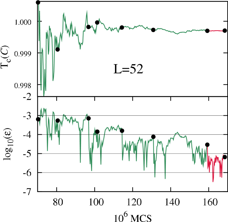
Figure 1: (color online). Upper panel: Evolution of the temperature of the maximum of the specific heat during the WL sampling, beginning from $f_{9}$ for a single run. The dots show where the modification factor was updated. Lower panel: Evolution of the logarithm of the checking parameter $\varepsilon$ during the same simulation.

According to Eq. (11) the critical adimensional temperature for the $q=3$ Potts model is given by

$$\frac{k_{B}T_{c}}{J}=\frac{1}{\ln(1+\sqrt{3})}=0.994972861...$$ (20)

Evaluating the thermodynamic quantities Eqs. (12)-(17) at this temperature and taking into account Eq. (19), we are able to determine $\frac{1}{\nu}$ by the slopes of the straight lines that we obtain with respect to $\ln L$. For each of these six slopes we calculate $\nu=1/(\frac{1}{\nu})$ with $\varDelta\nu=\varDelta(\frac{1}{\nu})/(\frac{1}{\nu})^{2}$ and take an average with unequal uncertainties wong over them. In Fig. 2 we present this set of lines. From the linear fits to these points we estimate that $\frac{1}{\nu}=1.20847(41)$, yielding ${\nu}=0.82759(98)$. Nevertheless these values represent the result of only one of the $10$ sets of finite-size scaling simulations which were carried out. Initially we run over all sets calculating $\nu$ in order to determine this exponent to the best precision.

At this point we take a moment to discuss which procedure should be adopted to calculate the mean value of these $10$ results, a single averaging or an average with unequal uncertainties. In order to investigate the behavior of the data under these two procedures, we grouped the five first sets in a large one and the last five in another large set. Taking the averages with unequal uncertainties we obtained $\nu=0.82272(26)$ and $0.81658(38)$, while if we take just single averages neglecting the error bars, we obtain $\nu=0.8230(19)$ and $0.8165(22)$, in each of these two large sets. One can see that the former procedure leads to unrealistic error bars, whereas the later yields results that intersect within $\pm 2\sigma$ errors. We therefore adopt the single averaging here and in all the further calculations. In Table 1 the fourth column displays the values obtained in each set and the final result in the last line: ${\nu}=0.8197(17)$.

Next, with the critical exponent $\nu$ accurately determined, we can use Eqs.(7)-(8) to evaluate the exponents $\frac{\beta}{\nu}$ and $\frac{\gamma}{\nu}$ by the slopes of the log-log plots. In Fig. 3 and Fig. 4 we show this finite-size scaling behavior for each exponent, obtaining $\frac{\beta}{\nu}=0.1298(28)$ and $\frac{\gamma}{\nu}=1.753(16)$, respectively. We then calculate $\beta=\nu\frac{\beta}{\nu}$ with $\varDelta\beta=\frac{\beta}{\nu}\varDelta\nu+\nu\varDelta\frac{\beta}{\nu}$, and similarly for $\gamma$ and $\varDelta\gamma$, obtaining $\beta=0.1063(23)$, and $\gamma=1.435(13)$. Again, these values were obtained at the first folder. In Table 1 we show the results for all sets and the best estimates in the last line, yielding $\beta=0.10811(77)$, and $\gamma=1.4459(31)$. Finally using the scaling relation given by Eq. (10) we determined the exponent $\alpha=2-2\beta-\gamma$ with $\varDelta\alpha=2\varDelta\beta+\varDelta\gamma$. These results are also displayed in Table 1 giving $\alpha=0.3379(28)$.

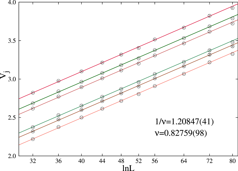
Figure 2: (color online) Size dependence of $V_{j}$ at the critical temperature. The slopes yield $1/\nu$.

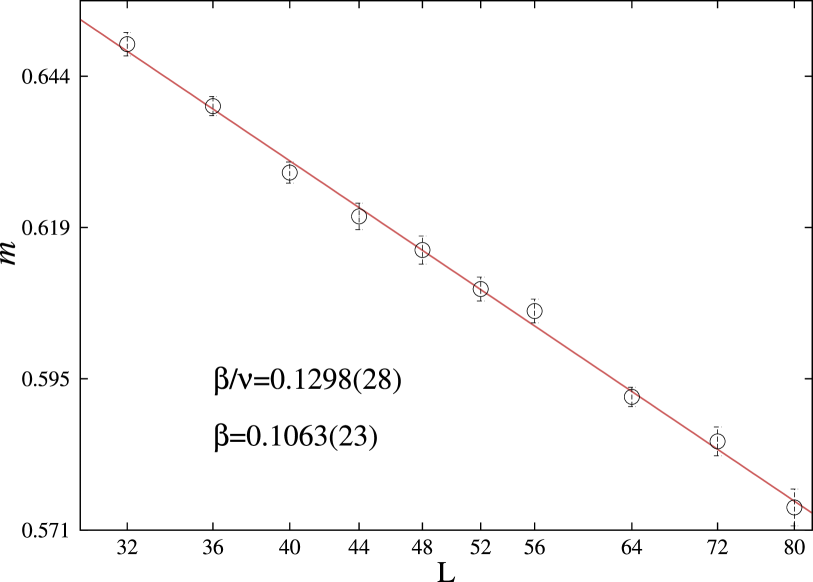
Figure 3: (color online) Log-log plot of size dependence of the magnetization at $T_{c}=0.994972861$.

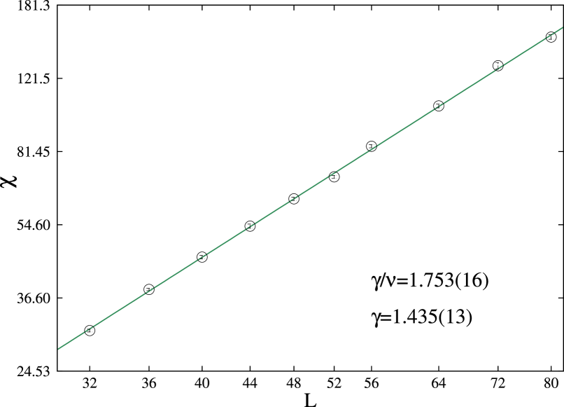
Figure 4: (color online) Log-log plot of size dependence of the susceptibility at $T_{c}=0.994972861$.

$\alpha$	$\beta$	$\gamma$	$\nu$		$\alpha$	$\beta$	$\gamma$	$\nu$
$q=3$ Potts model					$q=4$ Potts model
0.352(17)	0.1063(23)	1.435(13)	0.82759(98)		0.550(26)	0.0836(71)	1.283(12)	0.7123(13)
0.351(12)	0.1063(31)	1.4367(62)	0.82364(52)		0.541(18)	0.0951(35)	1.269(11)	0.7045(13)
0.340(14)	0.1120(32)	1.4361(83)	0.82068(56)		0.547(35)	0.0855(74)	1.282(20)	0.70907(91)
0.334(14)	0.1044(37)	1.4569(69)	0.81688(60)		0.539(24)	0.0950(43)	1.271(16)	0.7085(12)
0.350(16)	0.1093(39)	1.4315(91)	0.82601(47)		0.504(33)	0.0907(74)	1.315(19)	0.70185(77)
0.341(16)	0.1099(23)	1.440(12)	0.81797(88)		0.519(27)	0.0895(50)	1.302(17)	0.7041(12)
0.337(12)	0.1099(30)	1.4428(66)	0.82410(79)		0.538(24)	0.0946(66)	1.273(11)	0.7085(13)
0.336(12)	0.1053(33)	1.4535(62)	0.81632(63)		0.528(15)	0.0898(28)	1.292(10)	0.70671(83)
0.326(13)	0.1094(27)	1.4552(85)	0.81162(52)		0.521(23)	0.0958(50)	1.287(14)	0.7059(14)
0.329(10)	0.1071(27)	1.4563(50)	0.81249(45)		0.550(46)	0.056(12)	1.337(24)	0.7074(12)
0.3379(28)	0.10811(77)	1.4459(31)	0.8197(17)		0.5084(48)	0.0877(37)	1.3161(69)	0.7076(10)

Table 1: $q=3$ and $q=4$ Potts models: Ten finite-size scaling results for the exponents $\alpha$, $\beta$, $\gamma$, and $\nu$. The last line shows the average values over all the runs.

Method	$\alpha$	$\beta$	$\gamma$	$\nu$
$q=3$ Potts model
Conjectured value Wu1982	$\frac{1}{3}$	$\frac{1}{9}$	$\frac{13}{9}$	$\frac{5}{6}$
Kadanoff variational RG dasgupta	$0.326$	$0.107$	$1.460$	$0.837$
Monte Carlo RG rebbi	$0.352$	$0.101$	$1.445$	$0.824$
This work	$0.3379(28)$	$0.10811(77)$	$1.4459(31)$	$0.8197(17)$
$q=4$ Potts model
Conjectured value Wu1982	$\frac{2}{3}$	$\frac{1}{12}$	$\frac{7}{6}$	$\frac{2}{3}$
Kadanoff variational RG dasgupta	$0.488$	$0.091$	$1.330$	$0.756$
Duality invariant RG hu	$0.4870$	$-$	$-$	$0.7565$
This work	$0.5084(48)$	$0.0877(37)$	$1.3161(69)$	$0.7076(10)$

Table 2: Estimates of $\alpha$, $\beta$, $\gamma$, and $\nu$ compared to results obtained with other techniques and conjectured values.

For the $q=4$ Potts model the critical adimensional temperature is given by

$$\frac{k_{B}T_{c}}{J}=\frac{1}{\ln(1+\sqrt{4})}=0.910239226...$$ (21)

All the plots and finite-size scaling procedures are completely analogous to those we described above for the $q=3$ case. In Table 1 we display the results for the 10 folders and our final estimates yielding $\alpha=0.5084(48)$, $\beta=0.0877(37)$, $\gamma=1.3161(69)$, and $\nu=0.7076(10)$.

Such large repetitious handling of data for obtaining all these canonical averages and finite-size scaling extrapolations were possible only by using shell scripting AdvBashScr ; BGB2008 ; Robbins2005 ; Neves2008 ; Jargas2008-Shell . This is an exceptional tool for those who work with simulations.

As a final discussion, we compare in Table 2 our final estimates of the critical exponents to other well-established values. It is possible to see a good agreement for the $q=3$ case, especially between those obtained by numerical means. For the $q=4$ case, our results are below those of Refs. dasgupta ; hu . Notwithstanding our results for $\beta$, $\gamma$ and $\nu$ are closer to the conjectured ones when compared to these approaches. This is a clear indication that our procedure of carefully handling very accurate data obtained by an entropic sampling simulation is a powerful and reliable technique.

VI Conclusions

In this work we explored the static critical behavior of $q=3$ and $q=4$ Potts models within a high-precision and refined Wang-Landau procedure. All results are in very good agreement with those obtained from other well established approaches. The most striking conclusion from our analysis, in our opinion, is that it is possible to obtain reliable and very precise calculations of critical exponents from WL sampling provided that the appropriate implementations adopted in this work are made. Most important, the implementation of the present method remains as simple as the original idea of the WL algorithm. A further critical test of our algorithm would be provided by an analysis of the critical behavior of multi-parametric spin systems, which is a hard task for any conventional WL approach.

VII Acknowledgment

This work was supported by FUNAPE-UFG. We acknowledge the computer resources provided by LCC-UFG.

References

- (1) D.P. Landau, K. Binder, A Guide to Monte Carlo Simulations in Statistical Physics, Cambridge University Press, New York, USA, 2000.
- (2) W. Krauth, Statistical Mechanics: Algorithms and Computations, Oxford University Press, USA, 2006.
- (3) N. Metropolis, A. Rosenbluth, M. Rosenbluth, A. Teller and E. Teller, J. Chem. Phys. 21, 1087 (1953).
- (4) B. A. Berg and T. Neuhaus, Phys. Rev. Lett. 68, 9 (1992).
- (5) K. Hukushima and K. Nemoto, J. Phys. Soc. Jpn. 65, 1604 (1996).
- (6) F. Wang and D. P. Landau, Phys. Rev. Lett. 86, 2050 (2001); Phys. Rev. E 64, 056101 (2001).
- (7) P. Dayal, S. Trebst, S. Wessel, D. Wurtz, M. Troyer, S. Sabhapandit, and S. N. Coppersmith, Phys. Rev. Lett. 92, 097201 (2004).
- (8) D. P. Landau, S.-Ho Tsai, and M. Exler, Am. J. Phys. 72, 1294 (2004).
- (9) T. Nogawa, N. Ito, and H. Watanabe, Phys. Rev. E 84, 061107 (2011).Nogawa,T./Ito,N.//
- (10) C. J. Silva, A. A. Caparica and J. A. Plascak, Phys. Rev. E 73, 036702 (2006).
- (11) C. Yamaguchi and N. Kawashima, Phys. Rev. E 65, 056710 (2002).
- (12) C. Zhou and R. N. Bhatt, Phys. Rev. E 72, 025701 (2005).
- (13) R. E. Belardinelli and V. D. Pereyra, J. Chem. Phys. 127, 184105 (2007).
- (14) M.E.J. Newman and G.T. Barkema, Monte Carlo Methods in Statistical Physics, Claredon Press, Oxford, p. 120 (2001).
- (15) F.Y Wu, The Potts model, Rev. Mod. Phys. 54, 235 (1982).
- (16) Belardinelli, R.E., Pereyra, V.D., Dickman, R., and Lourenço, B.J., J. Stat. Mech., 2014, P07007 (2014).
- (17) A.A. Caparica and A.G. Cunha-Netto, Phys. Rev. E 85, 046702 (2012).
- (18) A.A. Caparica, Phys. Rev. E 89, 043301 (2014).
- (19) L.S. Ferreira and A.A. Caparica, Int. J. Mod. Phys. C 23, 1240012 (2012).
- (20) L.S. Ferreira, A.A. Caparica, M. A. Neto, and M. D. Galiceanu, J. Stat. Mech., 2012, P10028 (2012).
- (21) A. Malakis, A. Peratzakis, and N. G. Fytas, Phys. Rev. E 70, 066128 (2004).
- (22) A. Malakis, S.S. Martinos, I.A. Hadjiagapiou, N. G. Fytas, and P. Kalozoumis, Phys. Rev. E 72, 066120 (2005).
- (23) A. Malakis, A. N. Berker, I. A. Hadjiagapiou, and N.G. Fytas, Phys. Rev. E 79, 011125 (2009).
- (24) A. Malakis, A. N. Berker, I. A. Hadjiagapiou, N. G. Fytas, and T. Papakonstantinou, Phys. Rev. E 81, 041113 (2010).
- (25) A Monte Carlo sweep consists of spin-flip trials in the 2D Ising model or monomer moves in the homopolymer.
- (26) M.E. Fisher, in Critical Phenomena, edited by M. S. Green (Academic, New York, 1971).
- (27) M.E. Fisher and M.N. Barber, Phys. Rev. Lett. 28, 1516 (1972).
- (28) Phase Transitions and Critical Phenomena, edited by C. Domb and J. L. Lebowitz (Academic, New York, 1974), Vol. 8.
- (29) V. Privman, P.C. Hohenberg, and A. Aharony, in Phase Transitions and Critical Phenomena, eduted by C. Domb and J. L. Lebowitz (Academic, New York, 1991), Vol. 14, p. 1.
- (30) K. Chen,A.M. Ferrenberg, and D.P. Landau, Phys. Rev. B48, 3249 (1993).
- (31) A.A. Caparica, A. Bunker, and D.P. Landau, Phys. Rev. B 62, 9458 (2000); There is a misprinting in Eq.(3) in this paper, which should be .
- (32) S.S.M. Wong, Computational Methods in Physics and Engineering, 2nd edition, World Scientific Publishing Co. Pte. Ltd. (1997).
- (33) C. Dasgupta, Phys. Rev. B 15, 3460 (1977).
- (34) C. Rebbi, and R. H. Swendsen, Phys. Rev. B 21, 4094 (1980).
- (35) B. Hu, J. Phys. A 13, L321 (1980).
- (36) M. Cooper, “Advanced bash-scripting guide” (2012). Retrieved from http://www.tldp.org/LDP/abs/html/.
- (37) M. Garrels “Bash guide for beginners” (2008). Retrieved from http://www.tldp.org/LDP/Bash-Beginners-Guide/html/index.html.
- (38) A. Robbins and N.H.F. Beebe, “Classic Shell Scripting: Hidden Commands that Unlock the Power of Unix”, Oreilly Series, (O’Reilly 2005).
- (39) J.C. Neves, “Programação Shell Linux”, edição, (Brasport, 2008).
- (40) A.M. Jargas, “Shell Script Profissional” (Novatec, 2008).
- (41) M. Nauenberg, and D.J. Scalapino, Phys. Rev. Lett. 44, 837 (1980).
- (42) J. Salas ,and A. D. Sokal, J. Stat. Phys. 88, 567 (1997).
- (43) P. E. Theodorakis, and N. G. Fytas, Phys. Rev. E 86, 011140 (2012).