Interaction as stochastic noise

Interaction is so ubiquitous that imaging a world free from it is a difficult fantasy exercise. At the same time, in understanding any complex physical system, our ability of accounting for the mutual interaction of its constituents is often insufficient when not the restraining factor. Many strategies have been devised to control particle-particle interaction and explore the diverse regimes, from weak to strong interaction. Beautiful examples of these achievements are the experiments on Bose condensates Pollack et al. (2009); Dalfovo et al. (1999); Nguyen et al. (2014), or the recent experiments on the dynamics of spin chains Jurcevic et al. (2014); Richerme et al. (2014). Here I introduce another possibility, namely replacing the particle-particle interaction with an external stochastic field, and once again reducing the dynamics of a many-body system to the dynamics of single-particle systems. The theory is exact, in the sense that no approximations are introduced in decoupling the many-body system in its non-interacting sub-parts. Moreover, the equations of motion are linear, and no unknown external potential is inserted.

The idea of replacing the many-body system under investigation with a non-interacting doppelganger is not new. From a theoretical point of view, a starting idea has been to treat the interaction as an external perturbation. Interaction “dresses” the particles and new fundamental particles appear for the description of a physical phenomenon. This is the tenet of the Landau’s theory of the Fermi gas mapping a strongly interacting electron gas into a system of weakly interacting quasi-particles Mattuck (1992); Giuliani and Vignale (2005). More modern approaches replace the particle-particle interaction with an external effective potential, e.g., the Thomas-Fermi’s theory and the Hartree-Fock approximation Bransden and Joachain (1995) which have all converged now somewhat in the Density Functional Theory Hohenberg and Kohn (1964); Kohn and Sham (1965); Giuliani and Vignale (2005). The price to pay for this huge simplification is the inclusion of a unknown non-linear potential in the dynamics of the fictitious non-interacting system Giuliani and Vignale (2005); Dreizler and Gross (1990). Density functional theory has been instrumental in understanding many physical, chemical, and biological phenomena at the nano-scale and in augmenting the theoretical prediction potential.

With hindsight the results I will present in the following are not completely surprising: for example when dealing with magnetic systems, a common approximation consists in replacing the dynamics of spin operators with the dynamics of their quantum averages. Often, these averages have a random behavior since they mostly consist of the superposition of a static magnetic moment and small dynamical fluctuations.

In this Letter, I will show that this analogy is even more stringent and can be made exact for the case in which particles interact via a potential that depends on one operator of particle $i$ multiplied by an operator of particle $j$. Indeed, the dynamics of such a system is exactly equivalent to the dynamics of a system of non-interacting particles in the presence of known stochastic potentials. The dynamics of the many-body system is then recovered by constructing the proper wave-function or density matrix and averaging the results over the stochastic fields. This study finds direct application in the dynamics of arbitrary spin-chains and gives immediate access to the exact high-order correlation functions that recently have been probed experimentally Jurcevic et al. (2014); Richerme et al. (2014). Moreover, the results presented here open up the possibility of investigating the dynamics of large systems. It is well known indeed that the numerical solution of the equation of motion of the many-body density matrix, $\hat{\rho}$, is limited by its intrinsic large dimensionality which scales at least quadratically with the number of states one needs to consider, compared with the linear scaling of the wave-function. Our result shows that for certain cases, one can bring the exact dynamics down to the evaluation of $N$ relatively small density matrices, thus regaining a linear scaling. To give an estimate of the problem with the interacting system, with a chain of $N$ spin $1/2$, the exact many-body states belongs to a space of dimensionality $2^{N}$, and therefore the density matrix has dimension $2^{N}\times 2^{N}$. It should be then apparent that we can investigate numerically small chains, routinely up to $N\simeq 10-15$, after which the computer memory requirements will be prevailing. Our result brings down this requirement to store up to $N$ $2\times 2$ matrices.

Let us begin with considering a many-body quantum system, whose dynamics is determined by the many-body Hamiltonian

$$\hat{H}=\sum_{i}^{N}\hat{h}_{i}+\sum_{i<j}^{N}\lambda_{i,j}\hat{x}_{i}\otimes\hat{x}_{j},$$ (1)

where $h_{i}$ is a single particle Hamiltonian and $\hat{x}_{i}$ is some operator acting on the particle $i$, $\lambda_{i,j}$ the interaction constant between particle $i$ and particle $j$, and $N$ the total particle number. By Newton’s third law, the interaction constant is symmetric, i.e, $\lambda_{i,j}=\lambda_{j,i}$. The many-body density matrix of the system evolves according to the von Neumann’s equation

$$\hbar\partial_{t}\hat{\rho}(t)=-i\left[\hat{H}(t),\hat{\rho}(t)\right].$$ (2)

For simplicity, let us assume that the initial density matrix is the direct product of single particle density matrices

$$\hat{\rho}(t=0)=\bigotimes_{i=1,N}\hat{\rho}_{i}(t=0),$$ (3)

then we can find a set of $N^{2}$ independent white complex noises $\omega_{i,j}(t)$ for which the single particle density matrix $\hat{\rho}_{i}$ evolves according to 

$$\begin{split}\hbar d\hat{\rho}_{i}(t)=&-i\left[h_{i},\hat{\rho}_{i}(t)\right]dt\\ &+\sum_{j=1}^{N}\frac{\sqrt{\hbar\lambda_{i,j}}}{2}\left(\left[\hat{x}_{i},\hat{\rho}_{i}\right]d\omega_{i,j}-i\left\{\hat{x}_{i},\hat{\rho}_{i}\right\}d\omega^{*}_{j,i}\right)\end{split}$$ (4)

and the exact total density matrix is given by

$$\hat{\rho}(t)=\overline{\bigotimes_{i=1,N}\hat{\rho}_{i}(t)}$$ (5)

where the $\overline{\cdots}$ denotes the average over all the white noises. In Eqs. (2) and (4), $[\hat{A},\hat{B}]=\hat{A}\hat{B}-\hat{B}\hat{A}$ and $\{\hat{A},\hat{B}\}=\hat{A}\hat{B}+\hat{B}\hat{A}$ are the standard commutator and anti-commutator of any two operators, respectively. The white noises $\omega_{i,j}$ are complex Wiener processes that satisfy

$$\overline{d\omega_{i,j}^{*}d\omega_{k,p}}=2\delta_{i,k}\delta_{j,p}dt,$$ (6)

where $\delta_{i,k}=1$ if $i=k$ or vanishes otherwise Gardiner (1983); Gardiner and Zoeller (2000); Breuer and Petruccione (2002); Higham (2001). We prove Eq. (5) starting from Eqs. (4) in the Methods section.

Let me now discuss two important points. First, it may appear that the initial correlation between the particles is lost in this theory. This is not the case. Indeed, the following discussion can be generalized to the case in which the initial condition is given by $\hat{\rho}(0)=\bigotimes_{i=1,N}\sum_{k}\gamma_{k}\hat{\rho}_{i}^{k}(0),$ where ${\gamma_{k}}$ is a set of coefficients such that $\sum_{k}\gamma_{k}=1$, to ensure that if $\mathrm{tr}\hat{\rho}_{i}^{k}(0)=1$ for any $i$, then $\mathrm{tr}\hat{\rho}(0)=1$. The total density matrix in this case, owing to the linearity of the equation of motion, will then be given by $\hat{\rho}(t)=\sum_{k}\gamma_{k}\overline{\bigotimes_{i=1,N}\hat{\rho}^{k}_{i}(t)},$ where each $\hat{\rho}^{k}_{i}$ evolves according to Eq. (4) with initial condition $\hat{\rho}^{k}_{i}(0)$. For simplicity, in the following I will maintain that Eq. (3) is satisfied by the initial density matrices. The second point is the form of the particle-particle interaction: if any operator of particle $i$ commutes, or anti-commutes, with any operator of particle $j$ then one can always expand any two-particle interaction as a series of products of single particle operators like in Eq. (1). The theory we are putting forward then is useful for those case in which the particle-particle interaction is written as a finite sum of products of pairs of single-particle operators. Finally, it should be clear that even if the initial density matrix $\hat{\rho}_{i}(0)$ describes a real particle, its time evolution $\hat{\rho}_{i}(t)$ cannot be associated with the dynamics of a real particle. This is easily seen by the fact that Eq. (4) does not preserve either the positivity or the unitarity of $\hat{\rho}_{i}(t)$, even if we assume $\hat{\rho}_{i}(0)$ is a definite positive matrix of unitary trace. We will discuss later on how to reduce the many-body density matrix to a proper single-particle (reduced) density matrix that can be used to investigate the single-particle properties of the system.

The exact dynamics of the many-body density matrix usually contains a redundant amount of information. For practical purposes, it is usually more convenient to trace out some of the degrees of freedom and obtain the expectation value of single- or two-particle operators. Within this theory, this procedure emerges naturally from the definition of the operator $\hat{\rho}_{i}$. We have for example for the time evolution of the subsystem $j$,

$$\hat{\rho}_{j}^{R}(t)=\overline{\hat{\rho}_{j}(t)\prod_{i\not=j}\mathrm{tr}\hat{\rho}_{i}(t)},$$ (7)

where $\mathrm{tr}$ indicates the trace operation on the matrix $\hat{\rho}_{i}$. Notice that in general $\overline{\mathrm{tr}\hat{\rho}_{i}(t)}$ is a function of time, and we cannot expect that it equals 1 at all times. On the other hand, we expect that $\mathrm{tr}\hat{\rho}_{j}^{R}(t)=\mathrm{tr}\hat{\rho}(t)=1$ at all times, so that $\hat{\rho}_{j}^{R}$ does define a proper density matrix for the subsystem $j$ 

As a first example of application we consider the case of two interacting spins. We assume there is not any external magnetic field. The Hamiltonian for this simple system is $\hat{H}=\lambda\sigma_{1}^{z}\otimes\sigma_{2}^{z}$ where $\sigma_{i}^{z}$ is the $2\times 2$ third Pauli matrix. For simplicity and without any loss of generality we can set $\lambda=\hbar$. According to Eq. (4) we need to solve the two independent stochastic master equations

$$\begin{split}d\hat{\rho}_{1}=\frac{1}{2}\left[\sigma^{z}\cdot\hat{\rho}_{1}(d\omega_{12}-id\omega^{*}_{21})-\hat{\rho}_{1}\cdot\sigma^{z}(id\omega^{*}_{21}+d\omega_{12})\right],\\ d\hat{\rho}_{2}=\frac{1}{2}\left[\sigma^{z}\cdot\hat{\rho}_{2}(d\omega_{21}-id\omega^{*}_{12})-\hat{\rho}_{2}\cdot\sigma^{z}(id\omega^{*}_{12}+d\omega_{21})\right].\end{split}$$ (8)

One can easily prove that the solution of these two stochastic equations are

$$\hat{\rho}_{1}(t)=\left(\begin{array}[]{cc}e^{i\omega^{*}_{21}}\rho_{1}^{11}&e^{\omega_{12}}\rho_{1}^{12}\\ e^{-\omega_{12}}\rho_{1}^{21}&e^{-i\omega^{*}_{21}}\rho_{1}^{22}\end{array}\right).$$ (9)

Here, we have introduced explicitly the elements of the initial state $\rho_{1}^{ii}$. $\hat{\rho}_{2}(t)$ can be obtained from this expression by substituting $1\rightarrow 2$ in the subscript of the initial state, and by swapping $1\leftrightarrow 2$ in the subscript of $\omega$. Some straightforward algebra now leads to the expression of $\tilde{\rho}(t)$, and with the properties of the averages we will discuss in a moment, to the final expression for the total density matrix $\hat{\rho}(t)$. We can prove that the density matrix obtained in this way is identical to the one obtained by evaluating $\hat{\rho}(t)=\exp(-iHt)\hat{\rho}(0)\exp(iHt)$ where $\hat{\rho}(0)=\hat{\rho}_{1}(0)\otimes\hat{\rho}_{2}(0)$. To obtain these results, we need to evaluate the stochastic averages of two functions: namely, both $\exp(\omega_{12}+\omega_{21})$ and $\exp(\omega_{12}+i\omega^{*}_{12})$. To do that, we observe that for any real Wiener process, $p$, and any complex number, $\alpha$, we have $\overline{\exp(\alpha p)}=\exp(-\alpha^{2}t/2)$ . We easily then arrive at $\overline{\exp(\omega_{12}+\omega_{21})}=1$ and $\overline{\exp(\omega_{12}+i\omega^{*}_{12})}=\exp(-2it)$. We can now evaluate the reduced density matrix for the spin 1, $\hat{\rho}_{1}^{R}(t)$. Again with some straightforward algebra, and assuming that $\mathrm{tr}\hat{\rho}_{1}(0)=1$, we obtain

$$\begin{split}\hat{\rho}_{1}^{R}(t)=\left(\begin{array}[]{cc}\rho^{11}_{1}&\rho_{1}^{12}(t)\\ \left(\rho_{1}^{12}(t)\right)^{*}&\rho_{1}^{22}\end{array}\right)\end{split}$$ (10)

where $\rho_{1}^{12}(t)=\rho^{12}_{1}\left(\cos 2t+i(\rho_{2}^{11}-\rho_{2}^{22})\sin 2t\right)$. With the reduced density matrix we can therefore calculate the expectation value of any single spin observable, e.g., $\langle\sigma_{1}^{z}\rangle=\rho_{1}^{11}-\rho_{2}^{22}$ and $\langle\sigma^{x}_{1}\rangle=2\mathrm{Re}(\rho_{1}^{12})\cos(2t)-2\mathrm{Im}(\rho_{1}^{12})(\rho_{1}^{22}-\rho_{1}^{11})\sin(2t)$.

The generalization to a chain of $N$ interacting spins 1/2 therefore follows in the same footsteps. If the start with the Hamiltonian $\hat{H}=\sum_{i,j=1}^{N}\lambda_{i,j}\sigma_{i}^{z}\otimes\sigma_{j}^{z}$, with $\lambda_{i,i}=0$ and use Eq. (4), we obtain the single spin stochastic density matrix

$$\hat{\rho}_{i}(t)=\left(\begin{array}[]{cc}\rho_{i}^{11}e^{i\sum_{j=1}^{N}\sqrt{\lambda_{i,j}}\omega^{*}_{j,i}}&\rho_{i}^{12}e^{\sum_{j=1}^{N}\sqrt{\lambda_{i,j}}\omega_{i,j}}\\ \rho_{i}^{21}e^{-\sum_{j=1}^{N}\sqrt{\lambda_{i,j}}\omega_{i,j}}&\rho_{i}^{22}e^{-i\sum_{j=1}^{N}\sqrt{\lambda_{i,j}}\omega^{*}_{j,i}}\end{array}\right).$$ (11)

From this result, deriving the single spin reduced density matrix is now straightforward,

$$\begin{split}\hat{\rho}_{i}^{R}(t)=\overline{\prod_{\begin{subarray}{c}k=1\\ k\not=i\end{subarray}}^{N}\mathrm{tr}\hat{\rho}_{k}(t)\hat{\rho}_{i}(t)}=\left(\begin{array}[]{cc}\rho_{i}^{11}&f_{i}(t)\\ f_{i}(t)^{*}&\rho_{i}^{22}\end{array}\right),\end{split}$$ (12)

where we have introduced the functions $f_{i}(t)=\rho_{i}^{12}\prod_{k=1,~{}k\not=i}^{N}\left(\rho_{k}^{11}\exp(-2i\lambda_{ik}t)+\rho_{k}^{22}\exp(2i\lambda_{ik}t)\right)$. In the same way, we can build the 2-spin reduced density matrix starting from its definition $\hat{\rho}_{i,j}^{R}(t)=\overline{\prod_{\begin{subarray}{c}k=1\\ k\not=i,j\end{subarray}}^{N}\mathrm{tr}\hat{\rho}_{k}(t)\hat{\rho}_{i}(t)\otimes\hat{\rho}_{j}(t)}$. The knowledge of $\hat{\rho}_{i,j}^{R}(t)$ allows us to calculate the correlation functions that have been recently measured Richerme et al. (2014); Senko et al. (2014), in accordance to new theoretical results Foss-Feig et al. (2013); van den Worm et al. (2013). The present theory provides an easy way to reproduce and generalize those results.

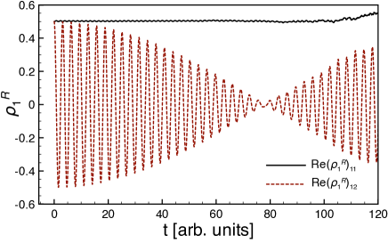
Figure 1: The time dynamics of the real parts of $(\rho_{1}^{R})_{11}$ and $(\rho_{1}^{R})_{21}$ calculated from Eqs. (7) and (4). As initial condition we have set the two spin in the “mixed” state. We have averaged over $10^{6}$ independent realizations of the white noises. For the calculation we have chosen $h_{1}=h_{2}=1$ and $\lambda=0.02$, and a time step, $\Delta t=0.01$. We can see that after $t\sim 100$ the finite number of realizations and the finite numerical accuracy in solving the stochastic differential equations are introducing an error in both $\rho_{1}^{11}$ and $\rho_{1}^{12}$.

We can investigate how the presence of a magnetic field, for example in the $\hat{x}$ direction affects the dynamics. To do that, we consider two interacting spins with the total Hamiltonian given by $\hat{H}=h_{1}\sigma_{1}^{x}+h_{2}\sigma_{2}^{x}+\lambda\sigma_{1}^{z}\otimes\sigma_{2}^{z}$. We can write down the stochastic equations of motion for the two single-spin density matrices, but their analytic solution of little use since $\sigma_{z}$ and $\sigma_{x}$ do not commute and we have to revert to a numerical solution of the equations of motion. In Fig. 1, we report the dynamics of a few elements of the density matrix $\hat{\rho}_{1}^{R}(t)$ calculated using Eqs. (7) and (4), after taking the average of $10^{6}$ independent realizations of the white noises. As initial condition we have assumed the two spins are in the mixed state, $\rho_{1}^{i,j}=\rho_{2}^{i,j}=1/2$ for any $i$ and $j$.

The possibility to measure in time, and locally the time evolution of the correlation between two spins has recently captured a lot of attention. Richerme et al. (2014); Jurcevic et al. (2014) In the experimental set-up, we could change the spin-spin interaction in such a way to explore the transition between a XY-model to Ising model. In particular, this possibility has been investigated in linear spin chains. Of particular interest is the spin-spin correlation function, since it can be seen as a way to measure the spin propagation speed and correlation time. To show how the present formalism can be applied to this case, we consider the Hamiltonian $\hat{H}=\sum_{i=1}^{N}h_{i}\sigma_{i}^{z}+1/2\sum_{i,j}^{N}\lambda_{ij}\left(\sigma_{i}^{x}\otimes\sigma_{j}^{x}\right)$, describing a chain of $N$ interacting spins in the presence of a static magnetic field $\vec{B}_{i}=(0,0,h_{i})$. In the following, we consider the case of a chain of $11$ spins, in the presence of a uniform magnetic field, $h_{i}=h$ for any $i$, and where the interaction if restricted to first neighbors. A quantity of interest for these systems is the time evolution of the correlation function, defined as $C_{i,j}=\langle\sigma^{z}_{i}\sigma^{z}_{j}\rangle-\langle\sigma^{z}_{i}\rangle\langle\sigma^{z}_{j}\rangle$. In Fig. 2 we report the time evolution of $C_{6,j}(t)$. We have chosen as initial condition that all the spin but $6$ are in a mixed state, while at $t=0$ the state of spin $6$ is up, that is $\rho_{6}^{1,1}=1$, $\rho_{6}^{1,2}=\rho_{6}^{2,1}=\rho_{6}^{2,2}=0$, while we have used $h=1$ and $\lambda_{ij}=0.01$ if $|i-j|=1$, or $0$ otherwise. We have chosen a time step of $\Delta t=0.002$ and averaged over 10000 realizations of the stochastic noise. It is seen that the correlation grows rapidly for the spin $5$ and $7$, while for the other spins, that are not directly connected with spin $6$, it remains rather small. This can be compared with the results of the experiments reported in Richerme et al. (2014); Jurcevic et al. (2014).

It is well known that the von Neumann equation is equivalent to the Schrödinger equation to almost any purpose in standard quantum mechanics Sakurai (1994); Gardiner and Zoeller (2000). It then appears natural to extend the result of this Letter to the many-body problem described by the time evolution of the many-body wave-function, $|\Psi(t)\rangle$. We can prove, following essentially in the footstep of the proof given for the many-body density matrix, than it is possible to find stochastic single-particle wave-functions $|\psi_{i}\rangle$ such that, if at the initial time $|\Psi(0)\rangle=\bigotimes_{i=1}^{N}|\psi_{i}(0)\rangle$, then for any subsequent time $|\Psi(t)\rangle=\overline{\bigotimes_{i=1}^{N}|\psi_{i}(t)\rangle}$. The states $\psi_{i}(t)$ evolve according to a stochastic Schrödinger equation Strunz et al. (2000); Gardiner and Zoeller (2000); Biele and D’Agosta (2012); D’Agosta and Di Ventra (2008, 2013) which has a form similar to Eq. (4). Interestingly, while the standard relation $\rho(t)=|\Psi(t)\rangle\langle\Psi(t)|$ is satisfied, there not exists a similar relation between the single-particles, i.e., in general we should expect that $\rho_{i}(t)\not=|\psi_{i}(t)\rangle\langle\psi_{i}(t)|$. Indeed, one can prove that $|\psi_{i}(t)\rangle\langle\psi_{i}(t)|$ has an equation of motion that does not reduce to Eq. (4). Finally, we would like to comment that a formalism based on the wave-function $|\psi_{i}\rangle$ seems limited, since it is not clear how one could possibly obtain information on the single-particle properties of the real many-body problem. In fact, if we start with the definition of $\hat{\rho}_{i}^{R}(t)$ from Eq. (7), and use the wave-function $|\Psi(t)\rangle$ instead we get,

$$\begin{split}\hat{\rho}_{j}^{R}(t)&=\mathrm{tr}\hat{\rho}(t)|_{\mathrm{but}~{}j}=\mathrm{tr}\left(|\Psi(t)\rangle\langle\Psi(t)|\right)|_{\mathrm{but}~{}j}\\ &=\mathrm{tr}\left(\overline{\bigotimes_{i=1}^{N}|\psi_{i}(t)\rangle}~{}\overline{\bigotimes_{i=1}^{N}\langle\psi_{i}(t)|}\right)_{\mathrm{but}~{}j}.\end{split}$$ (13)

It is therefore not possible to swap the trace operation with the average over the realizations of the stochastic noise, therefore precluding an alternative way to Eq. (7). Similar problems arise when one considers any $n$-body reduced density matrix as obtained from the single-particle stochastic wave-functions.

In conclusion, we have shown that the dynamics of a many-body system, with multiplicative two-body particle-particle interaction can be reduced to the investigation of the dynamics of $N$ single particle stochastic systems. We have shown how to calculate any reduced $n$-body properties starting from the solution of these stochastic dynamical equations. We have applied this formalism to the case of spin chains in the presence of a finite magnetic field.

Methods

Here we present the proof of Eq. (5), based on the Itô calculus Higham (2001); Gardiner and Zoeller (2000).

Proof. The proof of Eq. (5), and that $\hat{\rho}(t)$ follows the dynamics induced by the von Neumann’s equation (2) is a straightforward generalization of the results of Shao on the dynamics of a quantum system in contact with an external environment Shao (2004, 2010). Let us consider the stochastic total density matrix, $\tilde{\rho}(t)=\bigotimes_{i}\rho_{i}(t)$. According to Itô’s stochastic calculus, the dynamics of $\tilde{\rho}$ is determined by, $d\tilde{\rho}(t)=\sum_{j=1}^{N}\rho_{1,j}\otimes d\rho_{j}\otimes\rho_{j+1,N+1}+\sum_{k<j=1}^{N}\left(\rho_{1,k}\otimes d\rho_{k}\otimes\rho_{k+1,j}\otimes d\rho_{j}\otimes\rho_{j+1,N+1}\right),$ where we have introduced the short-hand notation $\rho_{i,j}=\bigotimes_{k=i}^{j-1}\rho_{k}.$ The proof that $\overline{\tilde{\rho}(t)}=\rho(t)$ then continues by using Eq. (4), Eq. (6), and $[\hat{x}_{i},\hat{\rho}_{j}]=0$ if $i\not=j$, to arrive at $d\overline{\tilde{\rho}(t)}=-i\left[\hat{H},\overline{\tilde{\rho}(t)}\right]dt.$ Due to the linearity of this equation of motion, and that by definition $\overline{\tilde{\rho}(0)}=\hat{\rho}(0)$, we conclude that $\overline{\tilde{\rho}(t)}=\hat{\rho}(t)$ at any time $t\geq 0$.$\square$

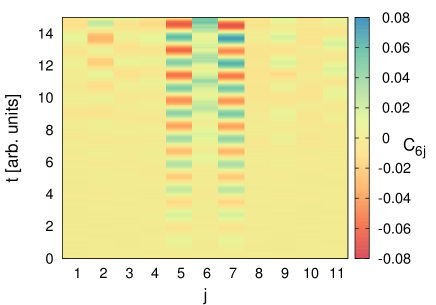
Figure 2: Dynamics of the correlation function $C_{6,j}(t)$ in time. We have chosen for the parameters $h=1$ and $\lambda=0.01$. All the spin but $6$ are in a mixed state, while spin $6$ starts in the state “up”. We have chosen a time step of $\Delta t=0.002$ and averaged over 10000 realizations of the stochastic noise.

References

- Pollack et al. (2009) S. E. Pollack, D. Dries, M. Junker, Y. P. Chen, T. A. Corcovilos, and R. G. Hulet, “Extreme tunability of interactions in a Li7 Bose-Einstein condensate,” Phys. Rev. Lett. 102, 090402 (2009).
- Dalfovo et al. (1999) F Dalfovo, S Giorgini, L P Pitaevskii, and S Stringari, “Theory of Bose-Einstein condensation in trapped gases,” Rev. Mod. Phys. 71, 463 (1999).
- Nguyen et al. (2014) Jason H V Nguyen, Paul Dyke, De Luo, Boris A Malomed, and Randall G Hulet, “Collisions of matter-wave solitons,” Nat. Phys. 10, 918–922 (2014).
- Jurcevic et al. (2014) P. Jurcevic, B. P. Lanyon, P. Hauke, C. Hempel, P. Zoller, R. Blatt, and C. F. Roos, “Quasiparticle engineering and entanglement propagation in a quantum many-body system,” Nature 511, 202–205 (2014).
- Richerme et al. (2014) Philip Richerme, Zhe-Xuan Gong, Aaron Lee, Crystal Senko, Jacob Smith, Michael Foss-Feig, Spyridon Michalakis, Alexey V. Gorshkov, and Christopher Monroe, “Non-local propagation of correlations in quantum systems with long-range interactions,” Nature 511, 198–201 (2014).
- Mattuck (1992) Richard D. Mattuck, A Guide to Feynman Diagrams in the Many Body Problem, 2nd ed. (Dover Publications, New York, 1992).
- Giuliani and Vignale (2005) Gabriele F. Giuliani and Giovanni Vignale, Quantum Theory of the Electron Liquid (Cambridge University Press, Cambridge, 2005).
- Bransden and Joachain (1995) B. H. Bransden and C. J. Joachain, Physics of Atoms and Molecules (Longman Scientific and Technical, Harlow, 1995).
- Hohenberg and Kohn (1964) P. Hohenberg and W. Kohn, “Inhomogeneous Electron Gas,” Phys. Rev. 136, B864–B871 (1964).
- Kohn and Sham (1965) Walter Kohn and L J Sham, “Self-Consistent Equations Including Exchange and Correlation Effects,” Phys. Rev. 140, A1133 (1965).
- Dreizler and Gross (1990) R M Dreizler and E K U Gross, Density Functional Theory (Springer-Verlag, Heidelberg, 1990).
- Note (1) Eq. (4) is not unique. Indeed, a family of equivalent equations can be easily obtained by shifting the weight of the interaction between the terms in the round bracket in the right hand side of that equation. The form chosen here keeps a balanced weight between the two terms. None of the physical results depend on the details of this choice.
- Gardiner (1983) C. W. Gardiner, Handbook of Stochastic Methods for Physics, Chemistry, and the Natural Sciences (Springer, 1983).
- Gardiner and Zoeller (2000) C. W. Gardiner and P. Zoeller, Quantum Noise, 2nd ed. (Springer, Berlin, 2000).
- Breuer and Petruccione (2002) Heinz-Peter Breuer and Francesco Petruccione, The Theory of Open Quantum Systems (Oxford University Press, New York, 2002).
- Higham (2001) Desmond J. Higham, “An Algorithmic Introduction to Numerical Simulation of Stochastic Differential Equations,” SIAM Rev. 43, 525–546 (2001).
- Note (2) We leave out the question if is also definitive positive. This point requires further investigation.
- Note (3) This can be easily proven by considering the stochastic differential equation solved by according to Ito’s calculus where is a real white noise, then taking the average, and solving the differential equation for obtained in this way.
- Senko et al. (2014) C. Senko, J. Smith, P. Richerme, A. Lee, W. C. Campbell, and C. Monroe, “Quantum simulation. Coherent imaging spectroscopy of a quantum many-body spin system.” Science 345, 430 (2014).
- Foss-Feig et al. (2013) Michael Foss-Feig, Kaden Hazzard, John Bollinger, and Ana Rey, “Nonequilibrium dynamics of arbitrary-range Ising models with decoherence: An exact analytic solution,” Phys. Rev. A 87, 042101 (2013).
- van den Worm et al. (2013) Mauritz van den Worm, Brian C Sawyer, John J Bollinger, and Michael Kastner, “Relaxation timescales and decay of correlations in a long-range interacting quantum simulator,” New J. Phys. 15, 083007 (2013).
- Sakurai (1994) J J Sakurai, Modern Quantum Mechanics (Addison Wesley, 1994).
- Strunz et al. (2000) Walter T. Strunz, Lajos Diósi, and Nicolas Gisin, “Non-Markovian Quantum State Diffusion and Open System Dynamics,” Lect. Notes Phys. 538, 271–280 (2000).
- Biele and D’Agosta (2012) Robert Biele and Roberto D’Agosta, “A stochastic approach to open quantum systems.” J. Phys. Condens. Matter 24, 273201 (2012).
- D’Agosta and Di Ventra (2008) Roberto D’Agosta and Massimiliano Di Ventra, “Stochastic time-dependent current-density functional theory: a functional theory of open quantum systems,” Phys. Rev. B 78, 165105 (2008).
- D’Agosta and Di Ventra (2013) Roberto D’Agosta and Massimiliano Di Ventra, “Foundations of stochastic time-dependent current-density functional theory for open quantum systems: Potential pitfalls and rigorous results,” Phys. Rev. B 87, 155129 (2013).
- Shao (2004) Jiushu Shao, “Decoupling quantum dissipation interaction via stochastic fields.” J. Chem. Phys. 120, 5053–6 (2004).
- Shao (2010) Jiushu Shao, “Dissipative dynamics from a stochastic perspective,” Chem. Phys. 370, 29–33 (2010).