Time Series Clustering using the Total Variation Distance with Applications in Oceanography

Abstract

An algorithm for determining stationary periods for time series of random sea waves is proposed in this work. This is a problem in which changes between stationary sea states are usually slow and segmentation procedures based on change-point detection frequently give poor results. The method is based on a new procedure for time series clustering, built on the use of the total variation distance between normalized spectra as a measure of dissimilarity. The oscillatory behavior of the series is thus considered the central characteristic for classification purposes. The proposed algorithm is compared to several other methods which are also based on features extracted from the original series and the results show that its performance is comparable to the best methods available and in some tests it performs better. This clustering method may be of independent interest.

Keywords: Spectral Analysis, Random Sea Waves, Hierarchical Clustering, Stationary Periods.

MSC classes: 62H30, 62M10, 62M15.

1 Introduction

An algorithm for determining stationary periods for time series of random sea waves is proposed in this work. This is a problem in which changes between stationary sea states are usually slow. The method is based on a new procedure for time series clustering, built on the use of the total variation distance between normalized spectra as a measure of dissimilarity. The oscillatory behavior of the series is thus considered the central characteristic for classification purposes.

Random processes have been used to model sea waves since the 1950’s, starting with the work of Pierson [30] and Longuet-Higgins [20]. Models based on random processes have proved useful, allowing the study of many wave features [see, e.g. 26]. A class of models often used to study sea waves in deep waters with standard conditions are stationary centered Gaussian processes [1, 26]. The stationarity hypothesis allows the use of Fourier spectral analysis to study the wave energy distribution as a function of frequency. In particular, this spectral analysis is related to several features of interest, such as the significant wave height ($H_{s}$) or the dominant or peak period ($T_{p}$), that can be computed from the spectral distribution [see, e.g. 26]. On the other hand, Gaussian models, beyond being a good first order approximation, allow obtaining explicit expressions for the distribution of parameters of interest. However, both hypotheses, stationarity and Gaussianity, have limitations. It is clear that in the medium/long-term the sea is not stationary. Thus, the use of stationary models is limited in time, depending on the specific sea conditions at the place of study. In other words, the sea state at a specific point can be regarded (or modeled) as an alternating sequence of stationary and transition periods (between the stationary periods).

The problem of duration of sea states is linked to the detection of change-points in time series. However, the methods employed to this effect usually assume that changes in the time series occur instantaneously or in a very brief period of time, which is not usually the case for waves, where changes take time to develop. This problem has been studied from different points of view. Ortega and Hernández [28] compared the results of using two methods, detection of changes by penalized contrasts proposed in Lavielle [17] and Lavielle and Ludeña [18] and the smoothed localized complex exponentials (SLEX), introduced by Ombao et al. [27], with unsatisfactory results. Soukissian and Samalekos [37] propose a segmentation method for significant wave height based on determining periods of stability, increase and decrease using time-series and local regression techniques. Hernández and Ortega [14] consider a method based on calculating mean values over moving windows, and using a fixed-width band to determine change points in the wave-height data. Other studies [38, 24, 23] have focused on the joint distribution of certain wave parameters, both from the point of view of estimation and from the point of view of simulation, with the purpose of obtaining duration distribution parameters through Monte Carlo methods. Jenkins [15] considers the problem from the perspective of estimating the fractal (Hausdorff) dimension.

As an application of time series clustering, we propose a new method for determining stationary periods for random waves, that takes into account the fact that transitions take some time to develop. The point of view switches from detecting change points to the identification of time intervals during which the behavior of the time series is stable. These time series are divided into 30-minute periods, a time interval which is usually considered to be long enough for a good estimation of the spectral density and short enough for stationarity to be a reasonable assumption. The clustering algorithm is then applied to the set of 30-minute intervals. If the clusters obtained are contiguous in time they are considered to be stationary intervals. The procedure also allows for the determination of transition intervals between successive stationary periods. Since one of our goals is to develop a method for determining stationary time intervals for sea waves that could be useful in Oceanography, the WAFO toolbox [6] in Matlab was used for all standard calculations regarding spectral densities and simulations from parametric spectral families.

In general, clustering is a procedure whereby a set of unlabeled data is divided into groups so that members of the same group are similar, while members of distinct groups differ as much as possible. The problem of clustering when the data points are time series has received a lot of attention in recent times. Liao [19] gives a revision of the field up to 2005 and Montero and Vilar [25] present an R package (TSclust) for time series clustering with a wide variety of alternative procedures. A thorough revision of the literature in recent years is outside the scope of this work, but the subject has found applications in diverse fields such as the identification of similar physicochemical properties of amino acid sequences [33], analysis of fMRI data [12], detection of groups of stocks sharing synchronous time evolutions with a view towards portfolio optimization [4], the identification of geographically homogeneous regions based on similarities in the temporal dynamics of weather patterns [5] and finding groups of similar river flow time series for regional classification [8], to name but a few.

According to Liao [19] there are three approaches to time series clustering: methods based on the comparison of raw data, feature-based methods, where the similarity between time series is gauged through features extracted from the data and methods based on parameters from models adjusted to the data. Our approach falls in the second group, and the feature used is the spectral density of the corresponding time series. The similarity between two time series is measured by the total variation distance (TV) between their normalized spectra. This distance is frequently used to compare probability measures, and requires the normalization of spectral densities, so that the integral of the normalized density is equal to one. This is equivalent to normalizing the time series so that its variance is equal to one. Thus, we focus on differences in the distribution of the variance as a function of frequency rather than differences in the total variance. The use of the TV distance for the analysis of differences in the context of spectral analysis of random waves was proposed by Álvarez-Esteban and Ortega [2] and also considered in Euán et al. [9, 10].

Once the spectra for the time series have been estimated and normalized, the TV distance between all pairs are calculated and used to build a dissimilarity matrix, which is then fed to an agglomerative hierarchical clustering algorithm. Several linkage criteria were used and Dunn’s index was employed for deciding the optimal number of clusters.

Many clustering algorithms have been devised for time series and to compare their performance Pértega and Vilar [29] proposed a series of tests. To gauge the efficiency of our algorithm the same tests were used. Since our interest lies in applications to random wave data, an additional test using families of spectral densities frequently used in Oceanography was also carried out. These tests show that, in most cases, the performance of the proposed algorithm compares with the best available, and in some cases it outperforms the rest.

The rest of this article is organized as follows: Section 2 introduces the TV distance, which will be used as the similarity measure between normalized spectral densities for the time series. Section 3 describes the clustering algorithm based on the TV distance. Section 4 reports results from a simulation study based partly on Pértega and Vilar [29] to compare the clustering algorithm with other methods. In Section 5 two types of applications are considered, first, using simulated data that includes transition periods the performance of the algorithm is assessed, and second, an application to real wave data is discussed in detail. The paper ends with conclusions about the results obtained.

2 Total Variation Distance

The total variation (TV) distance is one of the most widely used metrics between probability measures. Although it can be defined in general probability spaces, we will focus on the real line, $\mathbb{R}$. Given $P$ and $Q$, two probability measures in $\mathbb{R}$, the total variation distance between them is defined as

$$d_{TV}(P,Q)=\sup\{|P(A)-Q(A)|:A\in\mathcal{B}\}$$ (1)

where $\mathcal{B}$ is the class of the Borel sets on the real line.

One important property of the TV distance is that it is bounded between 0 and 1, being 1 the largest possible distance between two given probabilities. This property can be easily deduced from the definition. Obviously it is positive, and taking into account that for every Borel set $A$, $0\leq P(A),Q(A)\leq 1$ then, $0\leq|P(A)-Q(A)|\leq 1$ and the inequalities remain valid if we take the supremum over the sets in $\mathcal{B}$. A value of 1 for the distance can be attained if $P$ and $Q$ have disjoint supports.

This property is very useful in order to interpret distance values between two probabilities: values close to 1 mean that the two probabilities are quite different while distance values close to 0 mean that these probabilities are very similar, almost equal. A statistical test to contrast the null hypothesis that the TV distance between two probabilities is less or equal to a given threshold has been recently developed in Álvarez-Esteban et al. [3].

If $P$ and $Q$ have density functions (typically with respect to the Lebesgue measure $\mu$), $f$ and $g$, the TV distance between them can be computed [see, e.g., 22] using the following expression:

$$d_{TV}(P,Q)=1-\int_{-\infty}^{\infty}\min(f,g)\,d\mu=\frac{1}{2}\int|f-g|\,d\mu$$ (2)

and the supremum in (1) is attained with the set $A=\{f>g\}$.

This equation helps to graphically interpret the TV distance. If two densities $f$ and $g$, have TV distance equal to $1-\alpha$ this means that they share a common area of size $\alpha$. Thus, the more they overlap the closer they are. Figure 1 illustrates the case with two density functions and shows how to compute the TV distance. In this figure, the area of the orange region represents the TV distance, and is equal to the blue area, since the area under both densities is 1. Both colored regions represent the non-common part of the density functions, while the white area under the curves is the common part.

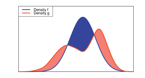
Figure 1: The TV distance measures the similarity between the two densities. The blue (orange) area is the value of the TV distance.

An alternative to the TV distance that is frequently considered is the Kullback-Leibler divergence between $P$ and $Q$, which is defined as

$$K(P,Q)=\int f\log\frac{f}{g}\,d\mu.$$

$K(P,Q)$ is not a true distance, but it has similar properties and is useful in many contexts. $K$ is always non-negative and takes the value 0 if and only if $P=Q$. However, if the set $\{f>0,g=0\}$ has strictly positive Lebesgue measure, which happens when $P$ is not dominated by $Q$, then $K(P,Q)=\infty$, while the TV variation distance between this measures is still bounded by 1. This situation, in which the K-L divergence is not useful, is feasible in the type of applications we will be considering. The TV distance is related to the K-L divergence through the following inequality, known as Pinsker’s inequality

$$\frac{1}{2}d_{TV}^{2}(P,Q)\leq K(P,Q).$$

A discussion of the use of the K-L divergence in discrimination and cluster analysis of time series using the spectral density can be found in Shumway and Stoffer [36]

3 Clustering using the spectral densities.

Our approach to stationary time series clustering is based on the spectral density as a feature that sums up the oscillatory behavior of the series around its mean value. In a physical context, e.g. when considering measurements of sea surface height at a fixed point, the spectrum of the time series is interpreted as the distribution of the energy as a function of frequency. The integral of the spectral density is (proportional to) the total energy present, and is, of course, the variance of the series. Thus a normalization of the spectral density corresponds to a consideration of the frequency distribution of the energy, disregarding the total energy present. Spectral densities that are similar after normalization correspond to times series that have similar oscillatory behavior around their mean values, but may differ in variance.

Several clustering methods based on spectral densities have been proposed in the literature. Shaw and King [34] consider periodograms normalized by dividing by the largest value and use the Euclidean distance between them to build a dissimilarity matrix, which is then fed to hierarchical clustering algorithm. Shumway [35] considers time-varying spectra within the framework of local stationarity, and uses the Kullback-Leibler discrimination measure, integrated over both frequency and time, to discriminate between seismic data coming from earthquakes and explosions. Caiado et al. [7] propose metrics based on the normalized periodogram for distinguishing stationary from non-stationary time series. Savvides et al. [33] use dissimilarity measures based on the cepstral coefficients, which are the coefficients in the Fourier expansion of the log spectrum. Maharaj and D’Urso [21] also use cepstral coefficients for a clustering algorithm based on fuzzy logic.

Kakizawa et al. [16] propose a general spectral disparity measure given by

$$d_{W}(X,Y)=\frac{1}{4\pi}\int_{-\pi}^{\pi}W\Big{(}\frac{f_{X}(\lambda)}{f_{Y}(\lambda)}\Big{)}d\lambda$$ (3)

where $f_{X}$ and $f_{Y}$ denote the spectral densities of the series $X$ and $Y$ respectively, and $W$ is a function that must satisfy certain regularity conditions in order to ensure that $d_{W}$ has the properties of a distance, except for the triangle inequality, and is thus a quasi-distance. With appropriate choices for $W$ (see Kakizawa et al. [16] for details) one can obtain the limiting spectral approximations to the Kullback-Leibler divergence and the Chernoff information in the time domain. They use these disparity measures with a hierarchical clustering algorithm and consider an application in seismology.

Our approach considers the normalized spectra of the time series as the feature of interest for clustering, and the TV distance between them is used to measure the similarity between two time series. The spectral densities were estimated using the inverse Fourier transform of the ACF, smoothed using a Parzen window with a bandwidth of length 100, with the toolbox WAFO in Matlab.

To choose the bandwidth, a series of test were performed. Using spectra from several parametric families of frequent use in Oceanography [see 13, 39, 40, 26] a Gaussian process was generated having a given spectral density, using WAFO. The data generated had a sampling frequency of 1.28 Hz. and corresponded to a 30-minute period, parameters that agree with the usual conditions for measurements in sea buoys. The empirical spectral density function was estimated using a range of bandwidths, and the TV distance between the original and the estimated spectral densities was calculated. This procedure was repeated 1000 times. The results showed that a bandwidth value around 100 was optimal.

The proposed clustering procedure is as follows:

• For each time series the spectral density is estimated and normalized.

• The total variation distance between the normalized spectral densities are calculated and used to build a dissimilarity matrix.

• This dissimilarity matrix is fed to an agglomerative hierarchical clustering algorithm. We considered two different linkage criteria: complete and average, and used the function agnes in R [31].

• To choose the number of clusters when no external indication was available, Dunn’s index was used. See section 5.2 for details.

4 Simulations

Pértega and Vilar [29] proposed two simulation tests to compare the performance of several clustering algorithms. These tests were reproduced here to compare the performance of the algorithm proposed in this article, with the best algorithms available. A third test based on simulated waves was added. In their study, Pértega and Vilar considered several dissimilarity criteria. For our purpose, we only included those that were not model-based and had the best results, plus the distance based on the cepstral coefficients (the Fourier coefficients of the expansion of the logarithm of the estimated periodogram). The dissimilarity criteria in the time domain included were:

• The distance between the estimated autocorrelation functions with uniform weights: $d_{ACFU}(X,Y)=\Big{(}\sum_{i}\big{(}\hat{\rho}_{i,X}-\hat{\rho}_{i,Y}\big{)}^{2}\Big{)}^{1/2}$.

• The distance between the estimated autocorrelation functions with decaying geometric weights: $d_{ACFG}(X,Y)=\Big{(}\sum_{i}p(1-p)^{i}\big{(}\hat{\rho}_{i,X}-\hat{\rho}_{i,Y}\big{)}^{2}\Big{)}^{1/2}$ with $0<p<1$.

Let $I_{X}(\lambda_{k})=T^{-1}\Big{|}\sum_{t=1}^{T}X_{t}e^{-i\lambda_{k}t}\Big{|}^{2}$ be the periodogram for time series $X$, at frequencies $\lambda_{k}=2\pi k/T,\ k=1,\dots,n$ with $n=[(T-1)/2]$, and $NI_{X}$ be the normalized periodogram, i.e. $NI_{X}(\lambda_{k})=I_{X}(\lambda_{k})/\hat{\gamma}_{0}^{X}$, with $\hat{\gamma}_{0}^{X}$ the sample variance of time series $X$. The dissimilarity criteria in the frequency domain considered were:

• The Euclidean distance between the estimated periodogram ordinates: $d_{P}(X,Y)=\frac{1}{n}\Big{(}\sum_{k}\big{(}I_{X}(\lambda_{k})-I_{Y}(\lambda_{k})\big{)}^{2}\Big{)}^{1/2}.$

• The Euclidean distance between the normalized estimated periodogram ordinates: $d_{NP}(X,Y)=\frac{1}{n}\Big{(}\sum_{k}\big{(}NI_{X}(\lambda_{k})-NI_{Y}(\lambda_{k})\big{)}^{2}\Big{)}^{1/2}.$

• The Euclidean distance between the logarithms of the estimated periodograms $d_{LP}(X,Y)=\frac{1}{n}\Big{(}\sum_{k}\big{(}\log I_{X}(\lambda_{k})-\log I_{Y}(\lambda_{k})\big{)}^{2}\Big{)}^{1/2}.$

• The Euclidean distance between the logarithms of the normalized estimated periodograms $d_{LNP}(X,Y)=\frac{1}{n}\Big{(}\sum_{k}\big{(}\log NI_{X}(\lambda_{k})-\log NI_{Y}(\lambda_{k})\big{)}^{2}\Big{)}^{1/2}.$

• The square of the Euclidean distance between the cepstral coefficients $d_{CEP}(X,Y)=\sum_{k}^{p}\big{(}\theta_{k}^{X}-\theta_{k}^{Y}\big{)}^{2}$ where, $\theta_{0}=\int_{0}^{1}\log I(\lambda)\mbox{d}\lambda$ and $\theta_{k}=\int_{0}^{1}\log I(\lambda)\cos(2\pi k\lambda)\mbox{d}\lambda$.

These dissimilarity measures were compared with the TV distance and the $L^{1}$ distance of the log of the normalized spectra, which is given by

$$d_{L^{1}}(f_{1},f_{2})=\frac{1}{2}\int|\log(f_{1}(\omega))-\log(f_{2}(\omega))|\mbox{d}\omega.$$

Three experiments were carried out, the first two were those proposed by Pértega and Vilar, and the third used simulated wave data. The steps for each experiment were:

1. Generate a group of time series of length $T$ that have some special characteristic, in order to have well-defined groups.

2. Calculate the dissimilarity matrix for each of the different measures. Here we fix some of the parameters as follows: For the ACFG and ACFU distances the maximum lag is $25$ and for the geometric weights we take $p=0.05$; for the CEP measure we take $p=128$ and the spectra were estimated as described in section 3.

3. The dissimilarity matrix is then used in a hierarchical clustering algorithm with the complete link.

4. The final groups are formed from the dendrogram by fixing the number $k$ of groups.

5. In order to evaluate the rate of success in the $m$-th iteration, the following index was used. Let $\{G_{1},\ldots,G_{g}\}$ and $\{C_{1},\ldots,C_{k}\}$, be the set of the $g$ real groups and a $k$-cluster solution, respectively. Then,

   $$\mbox{Sim}(C,G)=\frac{1}{g}\sum_{i=1}^{g}\max_{1\leq j\leq k}\mbox{Sim}(C_{j},G_{i}),$$

   where

   $$\mbox{Sim}(C_{j},G_{i})=\frac{2|C_{j}\cap G_{i}|}{|C_{j}|+|G_{i}|}.$$

   This was calculated for each trial and the average value is reported in the tables.

Experiment 1. In this experiment, a series of ARIMA models are considered. In each iteration, we simulate one realization of size $T=200$, from each of the following 12 ARIMA models proposed by Caiado et al. [7], six of which are stationary and six non-stationary.

$$\begin{array}[]{llll}\mbox{a) AR(1)}&\phi_{1}=0.9&\quad\mbox{g) ARIMA(1,1,0)}&\phi_{1}=-0.1\\ \mbox{b) AR(2)}&\phi_{1}=0.95,\phi_{2}=-0.1&\quad\mbox{h) ARIMA(0,1,0)}&\\ \mbox{c) ARMA(1,1)}&\phi_{1}=0.95,\theta_{1}=0.1&\quad\mbox{i) ARIMA(0,1,1)}&\theta_{1}=0.1\\ \mbox{d) ARMA(1,1)}&\phi_{1}=-0.1,\theta_{1}=-0.95&\quad\mbox{j) ARIMA(0,1,1)}&\theta_{1}=-0.1\\ \mbox{e) MA(1)}&\theta_{1}=-0.9&\quad\mbox{k) ARIMA(1,1,1)}&\phi_{1}=0.1,\theta_{1}=-0.1\\ \mbox{f) MA(2)}&\theta_{1}=-0.95,\theta_{2}=-0.1&\quad\mbox{l) ARIMA(1,1,1)}&\phi_{1}=0.05,\theta_{1}=-0.05\\ \end{array}$$

It is expected that clustering will divide the 12 series into two groups: stationary and non-stationary. Figure 2 (left) presents the spectral densities for the stationary processes. The figure shows that these spectra are not similar and so for the spectral methods we do not expect to get good results. Table 1 shows the rate of success, the ACFU gets the best results. A closer examination of the results, not included in the table, showed that when the spectra are not similar the TV distance works equally well.

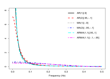
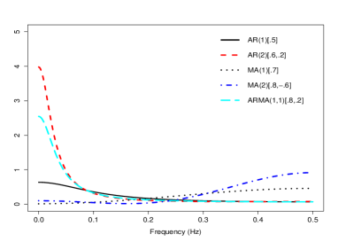
Figure 2: Spectra involved in experiment 1, stationary group (left) and in experiment 2 (right).

$T=200$
N	ACFG	ACFU	P	NP	LP	LNP	CEP	TV	L1
300	0.859	0.873	0.667	0.863	0.750	0.751	0.750	0.750	0.756
500	0.859	0.876	0.671	0.866	0.750	0.750	0.750	0.751	0.756
1000	0.861	0.878	0.674	0.870	0.750	0.750	0.750	0.751	0.756

Table 1: Results for Experiment 1. $T$ is the length of the series, $N$ is the number of replications. The best result for each value of $N$ is underlined.

Experiment 2. In this case, 5 different ARMA models were considered, but with a different objective. For each model four series are generated, and the clustering algorithm is then applied to the 20 samples, to see if they are able to recover the original groups. The number of groups in the clustering algorithm is set to 4 and 5. The 5 ARMA models have the following parameters: (a) AR(1): $\phi_{1}=0.5$, (b) MA(1): $\theta_{1}=0.7$, (c) AR(2): $\phi_{1}=0.6,\phi_{2}=0.2$, (d) MA(2): $\theta_{1}=0.8,\theta_{2}=-0.6$, (e) ARMA(1,1): $\phi_{1}=0.8,\theta_{1}=0.2$.

Figure 2 (right) shows the spectral densities for the five models. As can be seen, the spectra for the MA models are very similar so it may be difficult to distinguish them. In this case we take series of length $T=200,500$ and $1000$. The results are shown in Table 2.

$T=200$
$k$	N	ACFG	ACFU	P	NP	LP	LNP	CEP	TV	L1
4	100	0.530	0.473	0.432	0.469	0.722	0.701	0.613	0.599	0.703
4	500	0.536	0.484	0.440	0.480	0.718	0.695	0.612	0.599	0.699
5	100	0.660	0.620	0.515	0.610	0.939	0.736	0.719	0.742	0.925
5	500	0.663	0.620	0.518	0.611	0.928	0.739	0.711	0.739	0.922
$T=500$
$k$	N	ACFG	ACFU	P	NP	LP	LNP	CEP	TV	L1
4	100	0.592	0.568	0.490	0.561	0.733	0.732	0.711	0.664	0.730
4	500	0.585	0.561	0.492	0.558	0.733	0.732	0.708	0.667	0.731
5	100	0.745	0.683	0.561	0.687	0.998	0.798	0.820	0.852	0.995
5	500	0.741	0.685	0.566	0.683	0.999	0.798	0.817	0.846	0.996
$T=1000$
$k$	N	ACFG	ACFU	P	NP	LP	LNP	CEP	TV	L1
4	100	0.614	0.583	0.537	0.582	0.733	0.733	0.730	0.708	0.733
4	500	0.615	0.586	0.536	0.587	0.733	0.733	0.730	0.714	0.733
5	100	0.806	0.728	0.600	0.714	1.000	0.800	0.873	0.907	1.000
5	500	0.805	0.737	0.604	0.719	1.000	0.800	0.874	0.914	1.000

Table 2: Results for Experiment 2. $T$ is the length of the series, $k$ the number of clusters and $N$ the number of replications. The best result for each value of $T$ is underlined.

The LP distance works better for small or moderate-length series, however as $T$ increases the difference with the $L^{1}$ distance diminishes, and for $T=1000$ the results are equally good. If we only compare the spectral distances that do not use the logarithm, the TV distance is better, with a success rate that is between $10\%$ and $20\%$ higher than the rest, including the ACF distances.

The methods that involved the logarithm of the spectra did not perform well when the original spectral densities were very close and the shape was similar. In order to explore this in more detail, we performed a third simulation experiment, based on parametric spectra that are frequently used in Oceanography.

Experiment 3. The last experiment is based on two different JONSWAP (Joint North-Sea Wave Project) spectra. This is a parametric family of spectral densities which is frequently used in Oceanography, and is given by the formula

$$S(\omega)=\frac{g^{2}}{\omega^{5}}\exp(-5\omega_{p}^{4}/4\omega^{4})\gamma^{\exp(-(\omega-\omega_{p})^{2}/2\omega_{p}^{2}s^{2})}$$

where $g$ is the acceleration of gravity, $s=0.07$ if $\omega\leq\omega_{p}$ and $s=0.09$ otherwise; $\omega_{p}=\pi/T_{p}$ and $\gamma=\exp(3.484(1-0.1975(0.036-0.0056T_{p}/\sqrt{H_{s}})T_{p}^{4}/(H_{s}^{2})))$. The parameters for the model are the significant wave height $H_{s}$, which is defined as 4 times the standard deviation of the series, and the spectral peak period $T_{p}$, which is the period corresponding to the modal frequency of the spectrum. This spectral family was empirically developed after analysis of data collected during the Joint North Sea Wave Observation Project, JONSWAP, [13]. It is a reasonable model for wind-generated seas when $3.6\sqrt{H_{s}}\leq T_{p}\leq 5\sqrt{H_{s}}$.

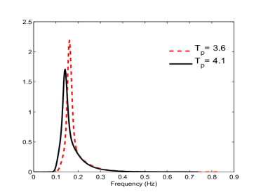
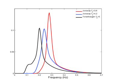
Figure 3: The JONSWAP spectra involved in experiment 3 (left) and the spectra involved in the simulations based on transitions (right).

The spectra considered both have significant wave height $H_{s}$ equal to $3$, the first has a peak period $T_{p}$ of $3.6\sqrt{H_{s}}$ while for the second $T_{p}=4.1\sqrt{H_{s}}$. Figure 3 (left) exhibits the JONSWAP spectra, showing that the curves are close to each other. This had the purpose of testing the performance of methods involving logarithms (LP and LNP), which had the best results in experiment 2, in a different scenario. For data coming from similar spectra, sampling variability in the estimation of the spectral densities may be enhanced by the logarithm and this may have the effect of making more difficult the correct identification of the two groups.

Four more dissimilarity measures were included in this experiment. These measures were considered by Pértega and Vilar [29] in their simulation study, but did not perform well in the previous experiments. Two of these measures come from (3) using $\widetilde{W}(x)=W(x)+W(1/x)$ with

$$W(x)=\log(\alpha x+(1-\alpha))-\alpha\log x)\quad\text{with }0<\alpha<1.$$

Vilar and Pértega [41] studied the asymptotic properties of this estimator when nonparametric estimators of the spectral densities obtained using local regression replace the spectral densities in (3). The two versions of this estimator considered in this study were $d_{W(DLS)}$, that uses local linear smoothers of the periodograms, obtained with least squares, and $d_{W(LK)}$ based on the exponential transformation of the local linear smoothers of the log-periodograms, obtained using maximum likelihood.

The other two dissimilarity measures are based on statistics that were originally introduced to test the equality of the log spectra of two processes (see Vilar and Pértega [41] for details). Let $m_{X}(\lambda)=\log(f_{X}(\lambda))$ and similarly for $Y$. The measures considered were

$$d_{GLK}(X,Y)=\sum_{k=1}^{n}\Big{[}Z_{k}-\hat{\mu}(\lambda_{k})-2\log\big{(}1+e^{(Z_{k}-\hat{\mu}(\lambda_{k}))}\big{)}\Big{]}-\sum_{k=1}^{n}[Z_{k}-2\log(1+e^{Z_{k}})],$$

where $Z_{k}=\log(I_{X}(\lambda_{k}))-\log(I_{Y}(\lambda_{k}))$, $\mu(\lambda_{k})=m_{X}(\lambda_{k})-m_{Y}(\lambda_{k})$ and $\hat{\mu}(\lambda_{k})$ is the local maximum log-likelihood estimator of $\mu(\lambda_{k})$ computed by local linear fitting, and

$$d_{ISD}(X,Y)=\int\big{(}\hat{m}_{x}(\lambda)-\hat{m}_{Y}(\lambda)\big{)}^{2}\,d\lambda,$$

where $\hat{m}_{X}(\lambda)$ and $\hat{m}_{Y}(\lambda)$ are the local linear smoothers of the log-periodograms, obtained using the maximum local likelihood in this case. It is important to observe

Four series from each spectrum were simulated with the purpose of testing whether the different criteria were able to recover the original groups. Table 3 gives the results. In this case the method proposed in this work performs better than the rest for short series, followed closely by ACFG. For medium sized series the best results correspond to $d_{W(LK)}$ while for long series $T=1000$ several methods, the TV distance among them, work equally well. In this experiment, in general, methods not using logarithms perform better than those that use it. It is important to observe that the methods that use the likelihood function are very slow for long series.

$T=100,\ k=2$
N	ACFG	ACFU	P	NP	LP	LNP	CEP	TV	L1	W(DLS)	W(LK)	ISD	GLK
100	0.783	0.769	0.623	0.764	0.669	0.662	0.654	0.786	0.641	0.636	0.750	0.742	0.721
500	0.785	0.771	0.624	0.762	0.671	0.655	0.669	0.790	0.657	0.641	0.736	0.731	0.711
$T=200,\ k=2$
N	ACFG	ACFU	P	NP	LP	LNP	CEP	TV	L1	W(DLS)	W(LK)	ISD	GLK
100	0.879	0.873	0.704	0.874	0.681	0.708	0.677	0.900	0.702	0.850	0.934	0.920	0.902
500	0.894	0.875	0.709	0.863	0.706	0.710	0.692	0.905	0.722	0.844	0.935	0.910	0.899
$T=1000,\ k=2$
N	ACFG	ACFU	P	NP	LP	LNP	CEP	TV	L1	W(DLS)	W(LK)	ISD	GLK
100	0.999	0.999	0.972	0.999	0.818	0.813	0.786	1.000	0.944	0.996	1.000	0.995	1.000
500	0.999	0.999	0.974	0.999	0.855	0.858	0.809	1.000	0.943	0.994	1.000	0.996	1.000

Table 3: Results for the Experiment 3. $T$ is the length of the series, $k$ the number of clusters and $N$ the number of replications. The best result for each value of $T$ is underlined.

5 Applications.

As was mentioned in the introduction, an interesting and important problem in Oceanography is the determination of stationary sea states. Consider a time series that represents the sea surface height at a fixed point as a function of time. If the sea state is stationary, the spectrum of this time series can be interpreted as the distribution of the energy as a function of frequency for the given sea state.

Typically, stationary sea states last for some time (hours or days), and then, due to changing weather conditions, sea currents, the presence of swell or other reasons, change to a different state. These changes do not occur instantaneously, but rather require a certain time to develop, during which there is a transition between the initial and final states. In this context, the usual segmentation methods that seek to determine change-points in a non-stationary time series do not work well, and a different point of view for the problem may be helpful: instead of looking for change-points, the idea is to identify short stationary intervals which have similar behavior, in terms of their spectral densities. If these intervals are contiguous in time, then it is reasonable to assume that they constitute a single (longer) stationary interval. The similarity is determined using the TV distance over normalized spectra and the clustering procedure described in section 3.

5.1 Simulated Data

Further simulation studies were carried out to assess the performance of the clustering algorithm in the presence of transition periods. The main objective was to gauge the performance when slow transitions between stationary periods are present in a data set. The simulations were carried out using the JONSWAP and Torsethaugen families of spectra. The latter is a family of bimodal spectra used in Oceanography, which accounts for the presence of swell and wind-generated waves, and was also developed to model spectra observed in North-Sea locations. Details can be found in Torsethaugen [39] and Torsethaugen and Haver [40].

In all cases the significant wave height ($H_{s}$) was set to 1; the simulated series starts with waves from a stationary period of 4 hours (JONSWAP spectrum with peak period $T_{p}=3.6$), then a transition lasting 3 hours to another stationary period (JONSWAP spectrum with $T_{p}=4.2$) and, after 4 hours, a new 3-hour transition to a third 4-hour stationary period (Torsethaugen spectrum with $T_{p}=5.0$). Figure 3 (right) shows the spectra involved in the experiment. One thousand replications of this scheme were simulated. The description of the method for simulating transition periods can be seen in Euán et al. [9].

	Cluster
	1	2	3	4	5
1	1000
2	1000
3	1000
4	1000
5	1000
6	1000
7	1000
8	999	1
9	981	19
10	533	467
11	174	826
12		906	88
13		487	513
14		72	926	2
15		45	950	5
16		41	953	6
17		47	947	6
18		44	952	4
19		43	952	5
20		43	950	7
21		45	951	4
22		44	951	5
23		29	939	32
24			464	536
25			127	873
26				824	176
27				449	551
28				21	979
29				1	999
30					1000
31				1	999
32				1	999
33				1	999
34				1	999
35				2	998
36					1000

(a)

	Cluster
	1	2	3
1	1000
2	1000
3	1000
4	1000
5	1000
6	1000
7	1000
8	1000
9	1000
10	980	20
11	815	185
12	565	435
13	188	812
14	5	995
15	1	999
16		1000
17		1000
18		1000
19		1000
20		1000
21		1000
22		1000
23		1000
24		863	137
25		585	415
26		297	703
27		57	943
28			1000
29			1000
30			1000
31			1000
32			1000
33			1000
34			1000
35			1000
36			1000

(b)

	Cluster
	1	2	3	4	5
1	1000
2	1000
3	1000
4	1000
5	1000
6	1000
7	1000
8	1000
9	991	1
10	559	441
11	168	832
12		872	126
13		421	579
14		68	931	1
15		49	950	1
16		49	950	1
17		49	950	1
18		49	950	1
19		49	950	1
20		49	950	1
21		49	950	1
22		49	950	1
23		41	945	14
24			498	502
25			126	873	1
26				815	185
27				415	585
28				5	995
29					1000
30					1000
31					1000
32					1000
33					1000
34					1000
35				1	999
36					1000

(c)

Table 4: Results for the simulated transition data using: a) Complete linkage function and $5$ groups, b) Complete linkage function and $3$ groups, c) Average linkage function and $5$ groups.

The simulated data was divided into 30-minute intervals and the corresponding spectra were estimated. Using these spectral densities, the clustering algorithm based on the TV distance was applied with two different linkage functions, complete and average. The algorithm was expected to recover five groups, the three stationary periods and two transitions. Table 4 shows the results for the 1000 replications. The row color stands for the original groups, for example, intervals $1$ to $8$, colored in dark orange, represent the first group. The column corresponds to the group assigned by the clustering algorithm.

Table 4(a) shows the results with the complete link function and 5 clusters. It can be seen that for the initial and final stationary periods, the algorithm almost always gives the correct result. For the central stationary period the success rate is around 95%. The algorithm has a harder time identifying the transition periods, which is reasonable since these are not homogeneous groups. In particular, intervals at the beginning and end of a transition period are classified as belonging to the nearest stationary period over 90% of the time in all cases. This is also reasonable since the transition is slow and due to the sampling variability in the estimation of the spectral densities, such small differences are difficult to detect. Table 4(c) shows the results for the average link function, which are similar.

One could argue that, in fact, the transition periods should not be considered as separate clusters, since they do not correspond to time intervals having homogeneous spectral densities, and in consequence one should only consider three groups. Table 4(b) shows the results in this case for the complete link function. Almost always, the stationary groups are correctly assigned to the same group. Transition intervals tend to be classified in the closest stationary group. These results could be used in a two-tier process, in which, in a given realization and using the results of the clustering algorithm, the intervals at the border would be tested to decide whether they really belong to the same group as the rest, or they should be considered as belonging to a transition period and moved outside the cluster. This idea will not be further developed in this work.

The initial division of the time series into 30-minute intervals determines the precision with which the stationary intervals can be determined. Shorter intervals will increase it but, on the other hand, using less data to estimate the spectral density will increase the statistical variability of the estimation. To test whether shorter time intervals would give good results, the simulated series were analyzed dividing them into 20-minute intervals. In general, when dealing with unimodal spectral densities such as those from the JONSWAP family, results were similar, but for bimodal densities in the Torsethaugen family results were worse. In this case the procedure has difficulty in clustering together the estimated spectra from this family, resulting in an important decrease in the number of correct classifications. For this reason, intervals of 30 minutes were used for the analysis of real data in the next section.

5.2 Real Data Analysis

Our starting point in this section is the idea that sea states at a fixed point on the sea surface can be modeled as a sequence of alternating stationary and transition periods. With this structure in mind and based on the results of the simulations shown in Section 5.1, we carried out a clustering analysis over a real data set in order to detect these periods.

We used real wave data obtained from the U. S. Coastal Data Information Program (CDIP) website. The data come from buoy 106 (51201 for the National Data Buoy Center), located in Waimea Bay, Hawaii, at a water depth of 200 m. and correspond to 192 30-minute intervals starting on January 1st., 2003, a total of 96 hours (4 days).

Figure 4 shows both significant wave height (solid) and spectral peak frequency (dashed) for this data set. It shows that $H_{s}$ starts with values around 2 m. and then, about the middle of the time interval, increases in a few hours to values around 3.7-4 m. where it remains for the rest of the period. On the other hand, the spectral peak frequency starts the period slightly increasing, then starts to decrease as $H_{s}$ increases, to remain low for the rest of the period.

The clustering analysis was carried out in two different ways. Initially the complete data set, comprising the 192 time intervals, was considered. Alternatively the data set was divided into two groups, group 1 including intervals 1 - 86 and group 2 intervals 87 - 192. A comparison of the results obtained in each case gives indications about the consistency of the proposed method and also allows for the evaluation of possible boundary effects in the segmentation procedure.

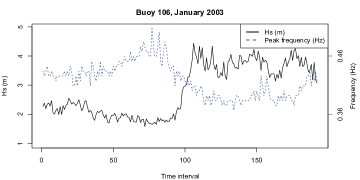
Figure 4: Significant wave height (solid) and peak frequency (dashed) for buoy 106, Jan 1st to 4th, 2003.

As in Section 5.1, for each 30-minute interval the spectral density was estimated and normalized, and the matrix of total variation distances between these spectra was calculated. This matrix is the input for the agglomerative hierarchical clustering procedure. We tried two of the main linkage functions: complete and average, with similar results.

Unlike the simulations of Section 5.1 where the number of clusters is known, now this number is unknown. In order to decide the appropriate number of clusters, $k$, to be considered in the analysis a suitable method should be chosen. A good review of available methods to assess the value of $k$ can be found, for example, in chapter 17 of Gan et al. [11]. In our case, as we have no external information about the number and definition of clusters we must select an internal method. Two methods were used, Dunn and Davies-Bouldin, with very similar results. We present here the results obtained with Dunn’s index, which is defined as

$$V_{D}(k)=\min_{1\leq i\leq k}\left\{\min_{i+1\leq j\leq k}\left(\frac{D(C_{i},C_{j})}{\max_{1\leq h\leq k}diam(C_{h})}\right)\right\},$$

where $k$ is the number of clusters, $D(C_{i},C_{j})$ is the distance between clusters $C_{i}$ and $C_{j}$, and $diam(C_{h})$ is the diameter of cluster $C_{h}$.

From the definition of $V_{D}$ it is clear that high values point to suitable values of $k$. The computation of this index was carried out using the clv package in R [31]. Among the available metrics to compute $D(C_{i},C_{j})$ and $diam(C_{h})$ the average was selected. The results for the three clustering procedures and the two linkage functions are shown in Figure 5. The main conclusion is that there is a good degree of agreement between the two linkage functions for each clustering procedure. Plot (a) for the clustering over the whole 192 intervals indicates the existence of 5 (average) or 6 (complete) groups. Dunn’s index in plot (b) for the first 86-time periods indicates clearly the existence of two groups, and finally, plot (c) for the second half of the period points to 3 (complete) or 4 (average) groups, depending on the linkage function.

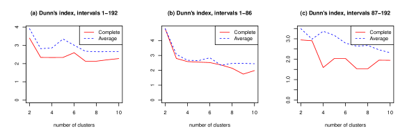
Figure 5: Dunn’s index for the three clustering processes using complete and average linkage functions: (a, left) intervals 1-192, (b, middle) intervals 1-86 and (c, right) intervals 87-192.

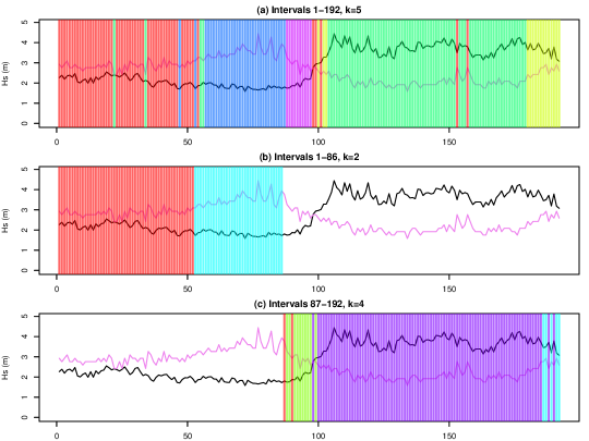
Figure 6: Clustering results using the average linkage function.

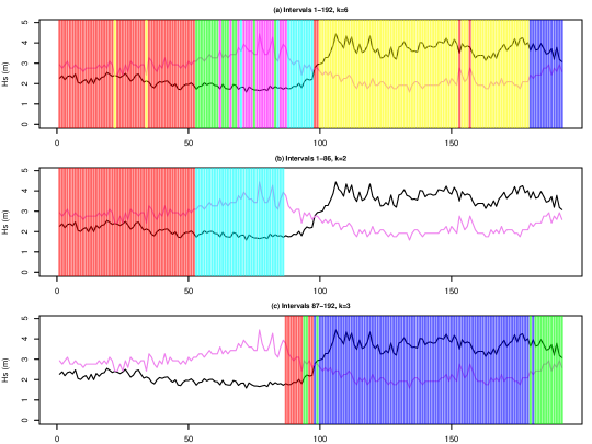
Figure 7: Clustering results using the complete linkage function.

After applying the hierarchical clustering algorithm, a silhouette analysis was performed to check for possible errors in the clustering process. In a hierarchical clustering algorithm, once an element has been assigned to a cluster, it cannot be reassigned to a different cluster, even if changes in the composition of the clusters as new elements are incorporated imply that it would have been better to assign this element to a different group.

The silhouette index, proposed by Rousseeuw [32], gives a measure of the adequacy of each point to its cluster. Let $a(i)$ be the average distance or dissimilarity of point $i$ with all the other elements within the same cluster, and let $b(i)$ be the smallest average dissimilarity of $i$ to any of the clusters to which $i$ does not belong. Then the silhouette index of $i$ is defined as

$$s(i)=\frac{b(i)-a(i)}{\max\{a(i),b(i)\}}$$

This index satisfies $-1\leq s(i)\leq 1$ for all $i$, and large positive values indicate that the element has been well classified while negative values point to misclassification. As a consequence the classification of intervals with negative silhouette index was revised. The reclassification only affected between 6 and 9 intervals, for the different cases considered.

Figures 6 and 7 show the results of the clustering procedure for the average and complete linkage functions, respectively, and $k$ chosen using Dunn’s index, after revision with the silhouette index. The first point to note in both figures is that, broadly speaking, the clustering procedure captures the time structure in the data. In other words, using only information about the TV distance between normalized spectral densities, the clustering procedure groups in the same cluster intervals that are contiguous in time, and this is valid except for a few intervals in each case.

Plot (a) of Figure 6 shows the groups for the whole time interval using $k=5$ clusters and the average linkage function. In this plot, the period of time between intervals 1 and 87, just before $H_{s}$ starts to increase, is essentially divided into two groups. The first cluster (red) comprises most of the initial 54 time intervals, with the exception of four of them, 22 and 34, which belong to the fourth cluster and 47 and 53, which belong to the second. It corresponds to a period of time during which both $H_{s}$ and $T_{p}$ are stable. The second cluster (57-87, in blue) includes the rest of the intervals in the first half and represents an uninterrupted sequence of time intervals, except for intervals 55 and 56, which are assigned to the fourth cluster. This is very similar to the clustering obtained for time intervals 1 - 86, represented in plot (b). In this case there are only two groups and the main difference with the first half of plot (a) is the starting point of the second cluster, which has moved to the left, to interval 53. The other difference is that now intervals 22, 34 and 47 are assigned to the first cluster, which becomes a single block, while the rest forms a second block.

The third group (88-97, purple) in plot (a) corresponds to the initial stages of growth for $H_{s}$, and is followed by 6 intervals, three of which (98, 99 and 101) belong to cluster 1 while the rest belong to cluster 5. The fourth cluster (104-179, green except 153 and 157) is the largest and includes almost all intervals of the period where $H_{s}$ oscillates around 3.7-4 m. There are two red intervals that break the time continuity of this cluster, 153 and 157, which belong to cluster 1. Finally, the fifth cluster (180-192, yellow) appears at the end of this last period, and is also an uninterrupted sequence of time intervals. Comparing with plot (c), which corresponds to intervals 87-192 divided into 4 groups, we see that the first interval (red) is classified as a cluster together with interval 90. In plot (a) interval 87 is the last in cluster 2 (dark blue). The second cluster (green) in plot (c) has similarities with cluster 3 in plot (a). The third cluster (purple) encompasses the fourth cluster (green) in plot (a) plus the segments included in cluster 1 (red) for this half of the data, as well as 8 intervals included in cluster 5 (yellow). Finally, cluster 4 (light blue) in plot (b) groups the rest of the intervals in cluster 5 (yellow) of plot (a).

As can be seen from this analysis, although there are some differences between the clustering obtained for the whole data set and those of the two halves, in general the agreement is very good, and those intervals in which the clustering differs, probably correspond either to transition intervals, such as the final intervals in plots (a) and (c), or to intervals in which temporary changes in the sea conditions (the presence of swell or local variations in the wind, for example) produce changes that disappear once these temporary conditions cease, as may be the case for intervals 22, 34, 153 and 157. A possible conclusion from this analysis is that there are three stable periods: 1 - 52, 57 - 87 and 104 - 179, and the other intervals correspond to transition periods.

A similar analysis can be done for the three plots in Figure 7, which correspond to the results with the complete linkage function. Plot (a) shows the complete time interval with 6 groups, while plots (b) and (c) correspond to the two halves with 2 and 3 clusters, respectively, as suggested by Dunn’s index.

For the first half, the first group in plots (a) and (b) is almost the same, except for intervals 22 and 34, which are assigned to a different group in plot (a). The assignement of intervals 52-86, however, is quite different. While in plot (b) they are all in a single cluster, in plot (a) they are divided into 3 different groups, none of which appears as a single block in time. As regards the second half, again the largest group (100-179) is very similar in both graphs, the difference being two intervals (153 and 157) in plot (a) that are assigned to a different group. The remaining intervals, 87-99 and 180-192 also show very similar structures in both cases.

Comparing now Figures 6 (a) and 7 (a) we see that the main differences lie in the interval 53-103, while the rest match very well. These differences are partly due to the fact that 5 clusters were chosen for the average linkage function, while for the complete the choice was 6 clusters. We also tried the complete linkage function with 5 clusters (not shown) and this shows more similarities with figure 6(a). On the other hand, the average linkage function seems to produce clusterings that are more homogeneous in time than those obtained using the complete link, although further research in this respect is needed.

6 Conclusions

In this paper, a new method for time series clustering was proposed. The method is based on using the total variation distance between normalized spectra as a measure of dissimilarity between time series. Simulation results (Sec. 4) show that the method has a performance that is comparable to the best clustering methods based on features extracted from the raw data, and in certain cases it performs better than the rest. Simulations (Sec. 5.1) also show that the method is capable of detecting stationary periods in situations where slow transitions between stationary states occur.

The method was used for the analysis of real sea wave data, measured at a fixed location, with the purpose of detecting stationary and transition periods. The results obtained using the average and complete linkage functions, presented in Sec. 5.2, show a reasonable agreement for the two linkage functions, taking into account that the number of clusters suggested by Dunn’s index is different. The analysis also shows that the results are consistent when the clustering method is applied over intervals of different length.

However, further research is needed to find a better criterion for choosing the number of clusters. Other aspects that need a closer look are the optimal length of the time window and the overlap interval for the automatic segmentation of longer data series, the use of trimming in order to robustify the clustering process and the possibility of using functional clustering with the spectral densities, instead of using the TV distance.

7 Acknowledgements

The software WAFO developed by the Wafo group at Lund University of Technology, Sweden, available at http://www.maths.lth.se/matstat/wafo was used for the calculation of all spectral densities and associated spectral characteristics. The data for station 106 were furnished by the Coastal Data Information Program (CDIP), Integrative Oceanographic Division, operated by the Scripps Institution of Oceanography, under the sponsorship of the U.S. Army Corps of Engineers and the California Department of Boating and Waterways (http://cdip.ucsd.edu/).

This work was partially supported by CONACYT, Mexico, Proyecto Análisis Estadístico de Olas Marinas, Fase II. J. Ortega wishes to thank Prof. Adolfo J. Quiroz for several fruitful conversations on the topic of this paper. P.C. Alvarez Esteban wishes to acknowledge CIMAT, A.C., the Spanish Ministerio de Ciencia y Tecnología, grants MTM2011-28657-C02-01 and MTM2011-28657-C02-02 and the Consejería de Educación de la Junta de Castilla y León, grant VA212U13 for their financial support.

References

- Aage et al. [1998] Aage, C.; Allan, T. D.; Carter, D.J.T.; Lindgren, G. and Olagnon, M. (1998) Oceans from Space. Éditions Ifremer, Brest, France.
- Álvarez-Esteban and Ortega [2012] Álvarez-Esteban, P.C. and Ortega, J. (2012). Changes in wave spectra and total variation distance. In Proc. 22nd Int. Offshore and Polar Engineering Conference, Vol. 3, 660–665.
- Álvarez-Esteban et al. [2012] Álvarez-Esteban, P.C.; del Barrio, E.; Cuesta-Albertos, J.A. and Matrán, C. (2012). Similarity of samples and trimming. Bernoulli, 18, 412–426.
- Basalto and De Carlo [2006] Basalto, N. and De Carlo, F. (2006) Clustering financial time series. In Hideki Takayasu, editor, Practical Fruits of Econophysics, 252–256. Springer Tokyo.
- Bengtsson and Cavanaugh [2008] Bengtsson, Thomas and Cavanaugh, Joseph E. (2008) State-space discrimination and clustering of atmospheric time series data based on Kullback information measures. Environmetrics 19, 103–121.
- Brodtkorb et al. [2000] Brodtkorb, P.A.; Johannesson, P.; Lindgren, G.; Rychlik, I.; Rydén, E. and Sjö, E. (2000) WAFO - a Matlab toolbox for analysis of random waves and loads. In Proc. 10th Int. Offshore and Polar Eng. Conf., Vol. III, 343–350, Seattle, USA.
- Caiado et al. [2006] Caiado, J.; Crato, N. and Peña, D. (2006). A periodogram-based metric for time series classification. Computational Statistics and Data Analysis, 50, 2668–2684.
- Corduas [2011] Corduas, M. (2011). Clustering streamflow time series for regional classification. Journal of Hydrology, 407, 73–80.
- Euán et al. [2013] Euán, C.; Ortega, J. and Álvarez-Esteban, P.C. (2013). Detecting changes in wave spectra using the total variation distance. In Proc. 23rd Int. Offshore and Polar Engineering Conference, Vol. 3, 824–830.
- Euán et al. [2014] Euán, C.; Ortega, J. and Álvarez-Esteban, P.C. (2014). Detecting stationary intervals for random waves using time series clustering. In Proc. 33rd Int. Conference on Ocean and Arctic Engineering, 1–7. ASME.
- Gan et al. [2007] Gan, G.; Ma, C. and Wu, J. (2007). Data clustering - Theory, Algorithms, and Applications. SIAM, Philadelphia.
- Goutte et al. [1999] Goutte, G.; Toft, P.; Rostrup, E; Nielsen, F. and Hansen, L.K. (1999) On clustering fMRI time series. NeuroImage, 9, 298–310.
- Hasselmann et al. [1973] Hasselmann, K.; Barnett, T.P.; Bouws, E.; Carlson, H.; Cartwright, D.E.; Enke, K.; Ewing, J.A.; Gienapp, H.; Hasselmann, D.E.; Kruseman, P. et al. (1973) Measurements of wind-wave growth and swell decay during the Joint North Sea Wave Project (JONSWAP). Ergnzungsheft zur Deutschen Hydrographischen Zeitschrift Reihe, A, Deutsches Hydrographisches Institut, 1973.
- Hernández and Ortega [2007] Hernández C., J.B. and Ortega, J. (2007). A comparison of segmentation procedures and analysis of the evolution of spectral parameters. In Proc. 17th. Int. Offshore and Polar Engineering Conference, Vol. 3, 1836–1842.
- Jenkins [2002] Jenkins, A.D. (2002) Wave duration/persistence statistics, recording interval, and fractal dimension. International Journal of Offshore and Polar Engineering, 12, 109–113.
- Kakizawa et al. [1998] Kakizawa, Y., Shumway, R.H. and Taniguchi, M. (1998) Discrimination and clustering for multivariate time series. Journal of the American Statistical Association, 93, 328–340.
- Lavielle [1998] Lavielle, M. (1998). Optimal segmentation of random processes. IEEE Transaction on Signal Processing, 46, 1365–1373.
- Lavielle and Ludeña [2000] Lavielle, M. and Ludeña, C. (2000) The multiple change-points problem for the spectral distribution. Bernoulli, 65, 845–869.
- Liao [2005] Liao, T.W. (2005). Clustering of time series data – a survey. Pattern Recognition, 38, 1857–1874.
- Longuet-Higgins [1957] Longuet-Higgins, M.S. (1957). The statistical analysis of a random moving surface. Philos. Trans. Roy. Soc. London, Ser. A, 249, 321–387.
- Maharaj and D’Urso [2011] Maharaj, E.A. and D’Urso, P. (2011). Fuzzy clustering of time series in the frequency domain. Information Sciences, 181, 1187–1211.
- Massart [2007] Massart, P. (2007). Concentration Inequalities and Model Selection. Springer, Berlin.
- Monbet et al. [2007] Monbet, V., Aillot, P. and Prevosto, M. (2007) Survey of stochastic models for wind and sea state time series. Probabilistic Engineering Mechanics, 22, 113–126.
- Monbet and Prevosto [2001] Monbet, V. and Prevosto, M. (2001). Bivariate simulation of non stationary and non gaussian observed processes. Application to sea state parameters. Applied Ocean Research, 23, 139–145.
- Montero and Vilar [2014] Montero, P. and Vilar, J.A. (2014). TSclust: an R package for time series clustering. J. Statistical Software, 62, pp. 43.
- Ochi [1998] Ochi, M.K. (1998). Ocean Waves. The Stochastic Approach. Cambridge Ocean Technology Series. Cambridge Univ. Press.
- Ombao et al. [2002] Ombao, H.; Raz, J.; Von Sachs, R. and Guo, W. (2002). The SLEX model of a non-stationary random process. Ann. Inst. Statist. Math., 52, 1–18.
- Ortega and Hernández [2006] Ortega, J. and Hernández C., J.B. (2006) A comparison of two methods for spectral analysis of waves. In Proc. 16th. Int. Offshore and Polar Engineering Conference, Vol. 3, 45–52.
- Pértega and Vilar [2010] Pértega, S. and Vilar, J. A. (2010). Comparing several parametric and nonparametric approaches to time series clustering: A simulation study. J. of Classification, 27, 333–362.
- Pierson [1955] Pierson, W. J. Jr. (1955). Wind-generated gravity waves. Advances in Geophysics, 2, 93–178.
- R Core Team [2015] R Core Team (2015). R: A Language and Environment for Statistical Computing. R Foundation for Statistical Computing, Vienna, Austria.
- Rousseeuw [1987] Rousseeuw, P.J. (1987). Silhouettes: a Graphical Aid to the Interpretation and Validation of Cluster Analysis. Computational and Applied Mathematics, 20, 53–65. doi:10.1016/0377-0427(87)90125-7.
- Savvides et al. [2008] Savvides, A.; Promponas, V.J. and Fokianos, K. (2008). Clustering of biological time series by cepstral coefficients based distances. Pattern Recognition, 41, 2398–2412.
- Shaw and King [1992] Shaw, C.T. and King, G.P. (1992) Using cluster analysis to classify time series. Physica D, 58, 288–298.
- Shumway [2003] Shumway, R.H. (2003) Time-frequency clustering and discriminant analysis. Probability and Statistics Letters, 63, 307–314.
- Shumway and Stoffer [2010] Shumway, Robert H. and Stoffer, David S. (2010) Time Series Analysis and Its Applications: With R Examples. Third Edition. Springer Texts in Statistics, Springer.
- Soukissian and Samalekos [2006] Soukissian, T.H. and Samalekos, P.E. (2006). Analysis of the duration and intensity of sea states using segmentation of significant wave height time series. In Proc. 16th. Int. Offshore and Polar Engineering Conference, Vol. 3, 45–52.
- Soukissian and Theochari [2001] Soukissian, T.H. and Theochari, Z. (2001). Joint occurrence of sea states and associated durations. In Proc. 11th. Int. Offshore and Polar Engineering Conference, Vol. 3, 33–39.
- Torsethaugen [1993] Torsethaugen, K. (1993) A two-peak wave spectrum model. In Proc. 18th. Int. Conference on Ocean, Offshore and Artic Engineering (OMAE), Vol II, 175–180.
- Torsethaugen and Haver [2004] Torsethaugen, K. and Haver, S. (2004). Simplified double peak spectral model for ocean waves. In Proc. 14th. Int. Offshore and Polar Engineering Conference, 23–28.
- Vilar and Pértega [2004] Vilar, J. A. and Pértega, S. (2004). Discriminant and cluster analysis for Gaussian stationary processes: Local linear fitting approach. J. of Nonparametric Statistics, 16, 443–462.