Superfield Effective Potential for the Supersymmetric Topologically Massive Gauge theory in Four Dimensions

Abstract

We explicitly calculate the one-loop kählerian effective potential for the supersymmetric topologically massive gauge theory in four dimensions which involves two gauge superfields, the usual scalar one and the spinor one originally introduced by Siegel, coupled to a chiral scalar matter.

I Introduction

It is well known (see f.e. SGRS ) that in a four-dimensional space-time, three types of constrained superfields exist, consisting of irreducible representations of the supersymmetry algebra, that is, chiral, antichiral and linear superfields. The scalar chiral and antichiral superfields are well studied being the basic ingredients of the Wess-Zumino model and many other field theories BuKu ; ourcourse . Another well-studied important example is a real gauge superfield which is a reducible one since it is unconstrained, represents itself as a natural superfield extension of the usual gauge field, being thus a basic ingredient for supergauge theories such as super-QED and super-Yang-Mills theory (for different aspects of supergauge theories, see SGRS ; BuKu ; ourcourse and many other textbooks). However, these models do not exhaust the set of physically interesting theories.

In this paper, we consider a model for a spinor chiral superfield coupled to an usual chiral matter. Originally, the spinor chiral superfield was introduced in Siegel where it was shown to correspond to the so-called tensor multiplet and to allow for introducing, first, a new supergauge model, and second, a topological mass term in the case of coupling of the spinor gauge superfield to the usual real gauge scalar superfield. One more interesting feature of this model is that the gauge invariant strength, corresponding to spinor chiral and antichiral superfields, is just a linear superfield, differently from the chiral one, occurring for the real scalar superfield SGRS . While in Siegel only the free theory has been considered, we study here its coupling to a chiral matter. Classical aspects of this model were discussed in Fe . An alternative coupling for the linear superfield and tensor multiplet has been discussed in JL , where some of its string-related aspects were considered (for applications of this multiplet see also the references therein). Using the previously developed superfield effective potential methodology WZ ; WZ1 ; GC ; SYM , we calculate the one-loop superfield effective potential for this theory. We emphasize that, up to now, there were no examples of quantum calculations involving the chiral spinor superfields.

The structure of the paper looks like follows. In the section II, we discuss the classical action of the chiral spinor gauge superfield, coupled to the usual scalar gauge superfield and a chiral matter. In the section III we calculate the one-loop effective potential in this theory, and the section IV contains the summary of our results.

II Supersymmetric topologically massive gauge theory

Let us start our study with the supersymmetric topologically massive gauge theory which will be used to find the one-loop Kählerian effective potential (KEP). In the pure gauge sector, we have Siegel

$$S_{G}=\frac{1}{2}\int d^{6}zW^{\alpha}W_{\alpha}-\frac{1}{2}\int d^{8}zG^{2}-m\int d^{8}zVG\ ,$$ (1)

where $m$ is a constant with mass dimension equal to 1, and

$$W_{\alpha}=i\bar{D}^{2}D_{\alpha}V\ ,\ G=-\frac{1}{2}(D^{\alpha}\psi_{\alpha}+\bar{D}^{\dot{\alpha}}\bar{\psi}_{\dot{\alpha}})\ ,$$ (2)

where $\psi_{\alpha}$, $\bar{\psi}_{\dot{\alpha}}$ are chiral and antichiral spinor superfield corresponding to the tensor multiplet SGRS , and $V$ is an usual real gauge superfield. Actually, $G$ is a linear superfield satisfying the relation $D^{2}G=\bar{D}^{2}G=0$. The superfield strengths $W_{\alpha}$, $G$, and the action (1) are invariant under the Abelian gauge transformations:

$$\delta V=i(\bar{\Lambda}-\Lambda)\ ,\ \delta\psi_{\alpha}=i\bar{D}^{2}D_{\alpha}L\ ,\ \delta\bar{\psi}_{\dot{\alpha}}=-iD^{2}\bar{D}_{\dot{\alpha}}L\ ,$$ (3)

where $\Lambda$ is a chiral superfield, and $\bar{\Lambda}$ is an antichiral one, and $L=\bar{L}$ is a real scalar one SGRS .

Let us show that the theory (1) describes a massive gauge theory. For this, let us extract the equations of motion by varying the action (1) with respect to the superfields $V$ and $\psi_{\alpha}$. Then, we get

$$\frac{\delta S_{G}}{\delta V} = iD_{\alpha}W^{\alpha}-mG=0\ ,$$ (4)

$$\frac{\delta S_{G}}{\delta\psi_{\alpha}} = \bar{D}^{2}D^{\alpha}G-imW^{\alpha}=0\ .$$ (5)

On the one hand, if we multiply eq. (4) by $\bar{D}^{2}D^{\beta}$ and use $\bar{D}^{2}D^{\beta}D_{\alpha}W^{\alpha}=\Box W^{\beta}$, we get

$$(\Box-m^{2})W^{\alpha}=0\ .$$ (6)

On the other hand, if we multiply eq. (5) by $D_{\alpha}$ and use $D_{\alpha}\bar{D}^{2}D^{\alpha}G=\Box G$, we get

$$(\Box-m^{2})G=0\ .$$ (7)

Therefore, from eqs. (6) and (7), we can conclude that the superfield strengths $W_{\alpha}$ and $G$ satisfy massive Klein-Gordon equations.

In order to perform quantum calculations, we must add to (1) a gauge-fixing term. In particular, we will consider the following one Siegel :

$$S_{GF}=-\frac{1}{2\alpha}\int d^{8}zV\{D^{2},\bar{D}^{2}\}V-\frac{1}{8\beta}\int d^{8}z(D^{\alpha}\psi_{\alpha}-\bar{D}^{\dot{\alpha}}\bar{\psi}_{\dot{\alpha}})^{2}\ ,$$ (8)

where $\alpha$ and $\beta$ are the gauge-fixing parameters. The ghosts are completely factorized since the theory is Abelian.

Now, let us introduce interaction between the (anti-)chiral scalar superfield and the gauge superfields BuKu . Under the usual gauge transformation, the chiral and antichiral matter superfields transform as SGRS

$$\Phi^{\prime}=e^{2ig\Lambda}\Phi\ ,\ \bar{\Phi}^{\prime}=\bar{\Phi}e^{-2ig\bar{\Lambda}}\ .$$ (9)

The interaction term that we will consider in this paper, which is invariant under the combined transformations (3) and (9), is given by Chris

$$S_{M}=\int d^{8}z\bar{\Phi}e^{2gV}\Phi e^{4hG}\ .$$ (10)

The coupling constants $g$ and $h$ have mass dimensions zero and $-1$, respectively. The model $S_{G}+S_{M}$ [see eqs. (1) and (10)] was considered in Fe in the study of the formation of cosmic strings.

It follows from this expression that the tree-level KEP is

$$K^{(0)}=\Phi\bar{\Phi}.$$ (11)

Finally, the supersymmetric topologically massive gauge theory that we will study in this work follows from (1), (8), and (10):

$$S = -\frac{1}{2}\int d^{8}zV(-D^{\alpha}\bar{D}^{2}D_{\alpha}+\frac{1}{\alpha}\{D^{2},\bar{D}^{2}\})V-\frac{1}{8}\int d^{8}z\Big{\{}\big{(}1+\frac{1}{\beta}\big{)}[\psi_{\alpha}D^{\alpha}D^{\beta}\psi_{\beta}$$ (12)

$$+\bar{\psi}_{\dot{\alpha}}\bar{D}^{\dot{\alpha}}\bar{D}^{\dot{\beta}}\bar{\psi}_{\dot{\beta}}]+2\big{(}1-\frac{1}{\beta}\big{)}\psi_{\alpha}D^{\alpha}\bar{D}^{\dot{\beta}}\bar{\psi}_{\dot{\beta}}\Big{\}}+\frac{m}{2}\int d^{8}zV(D^{\alpha}\psi_{\alpha}+\bar{D}^{\dot{\alpha}}\bar{\psi}_{\dot{\alpha}})$$

$$+\int d^{8}z\bar{\Phi}e^{2gV}\Phi e^{-2h(D^{\alpha}\psi_{\alpha}+\bar{D}^{\dot{\alpha}}\bar{\psi}_{\dot{\alpha}})}\ ,$$

where we explicitly wrote the gauge superfields.

The standard method of calculating the effective action is based on the methodology of the loop expansion BO . To do this, we make a shift $\Phi\rightarrow\Phi+\phi$ in the superfield $\Phi$ (together with the analogous shift for $\bar{\Phi}$), where now $\Phi$ is a background (super)field and $\phi$ is a quantum one. We assume that the gauge superfields $V$, $\psi_{\alpha}$, and $\bar{\psi}_{\dot{\alpha}}$ are quantum. In order to calculate the effective action at the one-loop level, we have to keep only the quadratic terms in the quantum superfieds. By using this prescription, we get from (12)

$$S_{2}[\bar{\Phi},\Phi;\bar{\phi},\phi,\psi_{\alpha},\bar{\psi}_{\dot{\alpha}},V]=S_{q}+S_{int}\ ,$$ (13)

$$S_{q}=\frac{1}{2}\int d^{8}z\big{[}-V\Box(\Pi_{1/2}+\frac{1}{\alpha}\Pi_{0})V-\frac{1}{4}\big{[}\big{(}1+\frac{1}{\beta}\big{)}(\psi_{\alpha}D^{\alpha}D^{\beta}\psi_{\beta}+\bar{\psi}_{\dot{\alpha}}\bar{D}^{\dot{\alpha}}\bar{D}^{\dot{\beta}}\bar{\psi}_{\dot{\beta}})$$

$$\ \ \ \ +2\big{(}1-\frac{1}{\beta}\big{)}\psi_{\alpha}D^{\alpha}\bar{D}^{\dot{\beta}}\bar{\psi}_{\dot{\beta}}\big{]}+2\bar{\phi}\phi\big{]}\ ,$$ (14)

$$S_{int}=\frac{1}{2}\int d^{8}z\big{\{}(m-8gh\bar{\Phi}\Phi)V(D^{\alpha}\psi_{\alpha}+\bar{D}^{\dot{\alpha}}\bar{\psi}_{\dot{\alpha}})+2(2g)\bar{\Phi}V\phi+2(2g)\Phi\bar{\phi}V$$

$$\ \ \ \ +(2g)^{2}\bar{\Phi}\Phi V^{2}-4h\bar{\Phi}(D^{\alpha}\psi_{\alpha}+\bar{D}^{\dot{\alpha}}\bar{\psi}_{\dot{\alpha}})\phi-4h\Phi\bar{\phi}(D^{\alpha}\psi_{\alpha}+\bar{D}^{\dot{\alpha}}\bar{\psi}_{\dot{\alpha}})$$

$$\ \ \ \ +(2h)^{2}\bar{\Phi}\Phi[(D^{\alpha}\psi_{\alpha})D^{\beta}\psi_{\beta}+(\bar{D}^{\dot{\alpha}}\bar{\psi}_{\dot{\alpha}})\bar{D}^{\dot{\beta}}\bar{\psi}_{\dot{\beta}}+2(D^{\alpha}\psi_{\alpha})\bar{D}^{\dot{\alpha}}\bar{\psi}_{\dot{\alpha}}]\big{\}}\ ,$$ (15)

where the irrelevant terms were omitted, including those involving covariant derivatives of the background (anti-)chiral superfields. Moreover, we used the projection operators $\Pi_{1/2}\equiv-\Box^{-1}D^{\alpha}\bar{D}^{2}D_{\alpha}$ and $\Pi_{0}\equiv\Box^{-1}\{D^{2},\bar{D}^{2}\}$.

The one-loop approximation does not depend on how we break the Lagrangian into free and interacting parts Coleman . However, by convenience, we will extract the propagators from the terms that are independent of the background superfields and the vertices from the ones in which the quantum superfields interact with the background ones.

In the gauges $\alpha=0$ and $\beta=-1$, we obtain from $S_{q}$ the propagators

$$\langle V(1)V(2)\rangle=-\frac{1}{p^{2}}(\Pi_{1/2})_{1}\delta_{12}\ ,\ \langle\psi_{\alpha}(1)\bar{\psi}_{\dot{\alpha}}(2)\rangle=\frac{2p_{\alpha\dot{\alpha}}}{p^{4}}\delta_{12}\ ,\ \langle\phi(1)\bar{\phi}(2)\rangle=\frac{1}{p^{2}}\delta_{12}\ .$$ (16)

Before we start the calculation of the one-loop supergraphs, we first notice from (II) that there is a factor $D^{\alpha}\bar{D}^{2}$ in a vertex at one end of the propagator $\langle\psi_{\alpha}(1)\bar{\psi}_{\dot{\alpha}}(2)\rangle$, and there is a factor $\bar{D}^{\dot{\alpha}}D^{2}$ in the other vertex at the other end of the same propagator. Here the factors $\bar{D}^{2}$ and $D^{2}$ are present in the vertices due to the chirality (antichirality) of the superfield $\psi_{\alpha}$ ($\bar{\psi}_{\dot{\alpha}}$) just as in the usual Wess-Zumino model, because of the properties of the variational derivatives with respect to the chiral superfields (see SGRS ; BuKu ; ourcourse ), and the $D^{\alpha}$, $\bar{D}^{\dot{\alpha}}$ arise from the explicit form of the vertices. It is convenient to go from the above used formulation of propagators where the derivatives $D^{2}$, $\bar{D}^{2}$ are associated with the vertices, to a formulation where these derivatives are incorporated into the propagators (these two manners to introduce the Feynman supergraphs exist also in the Wess-Zumino model, see f.e. SGRS ). In other words, we associate the covariant derivatives with the propagator $\langle\psi_{\alpha}(1)\bar{\psi}_{\dot{\alpha}}(2)\rangle$ (instead to the vertices) and defining a new scalar field $\psi=D^{\alpha}\psi_{\alpha}$ with the propagator:

$$\langle\psi(1)\bar{\psi}(2)\rangle\equiv D^{\alpha}_{1}\bar{D}^{2}_{1}\bar{D}^{\dot{\alpha}}_{2}D^{2}_{2}\langle\psi_{\alpha}(1)\bar{\psi}_{\dot{\alpha}}(2)\rangle=2(\Pi_{1/2})_{1}\delta_{12}\ ,$$ (17)

where we used the fact that $\bar{D}^{\dot{\alpha}}_{2}D^{2}_{2}\delta_{12}=-D^{2}_{1}\bar{D}^{\dot{\alpha}}_{1}\delta_{12}$, and the factors $D^{2}$, $\bar{D}^{2}$ emerged due to properties of variational derivatives. We can also apply the same reasoning for the propagator $\langle\phi(1)\bar{\phi}(2)\rangle$ and for the vertices involving the scalar (anti-)chiral superfields.

In summary, by transferring all covariant derivatives from the vertices (II) to the propagators (16), we get

$$\langle V(1)V(2)\rangle = -\frac{1}{p^{2}}(\Pi_{1/2})_{1}\delta_{12}\ ,$$ (18)

$$\langle\psi(1)\bar{\psi}(2)\rangle = \langle\bar{\psi}(1)\psi(2)\rangle=2(\Pi_{1/2})_{1}\delta_{12}\ ,$$ (19)

$$\langle\phi(1)\bar{\phi}(2)\rangle = -(\Pi_{-})_{1}\delta_{12}\ ,\ \langle\bar{\phi}(1)\phi(2)\rangle=-(\Pi_{+})_{1}\delta_{12}\ ,$$ (20)

where $\Pi_{-}\equiv\Box^{-1}\bar{D}^{2}D^{2}$ and $\Pi_{+}\equiv\Box^{-1}D^{2}\bar{D}^{2}$ are projection operators. These propagators will connect the following new vertices:

$$\tilde{S}_{int} = \frac{1}{2}\int d^{8}z\big{\{}2MV(\psi+\bar{\psi})+2(2g)\bar{\Phi}V\phi+2(2g)\Phi\bar{\phi}V+(2g)^{2}\bar{\Phi}\Phi V^{2}$$ (21)

$$-4h\bar{\Phi}(\psi+\bar{\psi})\phi-4h\Phi\bar{\phi}(\psi+\bar{\psi})+(2h)^{2}\bar{\Phi}\Phi[\psi^{2}+\bar{\psi}^{2}+2\psi\bar{\psi}]\big{\}}\ ,$$

where $M\equiv\frac{1}{2}(m-8gh\bar{\Phi}\Phi)$. Therefore, now the vertices involve only scalar superfields.

In the next section, we will perform the calculations of the one-loop supergraphs using the propagators (18-20), written in terms of projection operators, and the vertices (21), written only in terms of scalar superfields, instead of the original propagators (16) and the original vertices (II).

III One-loop calculations

Now, let us start the calculations of the one-loop supergraphs contributing to the KEP. Since $\Pi_{1/2}\Pi_{-}=\Pi_{-}\Pi_{1/2}=\Pi_{1/2}\Pi_{+}=\Pi_{+}\Pi_{1/2}=0$, it follows from (18-20) that there can be no mixed contributions containing both gauge and matter propagators at one-loop order. Therefore, the basic supergraphs contributing to the effective action in the theory under consideration are of three types: first, those with internal lines composed of propagators $\langle\psi(1)\bar{\psi}(2)\rangle$ only; second, those composed of propagators $\langle V(1)V(2)\rangle$ only; third, those involving alternating propagators $\langle\psi(1)\bar{\psi}(2)\rangle$ and $\langle V(1)V(2)\rangle$. In our graphical notation, the dashed line is for $<\psi\bar{\psi}>$ propagator, the wavy line is for $<VV>$ propagator, and the double one is for $\Phi$ or $\bar{\Phi}$ background fields.

Figure 1: One-loop supergraphs composed by propagators $\langle\psi(1)\bar{\psi}(2)\rangle$.

It is easy to verify that the contribution to the effective action generated by the sum of supergraphs at the Fig. 1, with simple propagators (19), and the vertices $2(2h)^{2}(\Phi\bar{\Phi})\psi\bar{\psi}$ is zero. Indeed, it is equal to

$$\Gamma_{0}=\sum\limits_{n=1}^{\infty}\frac{1}{2n}[4(2h^{2})\Phi\bar{\Phi}<\psi\bar{\psi}>]^{n},$$ (22)

where the coefficient 4 is caused by two different contractions. Using the explicit form of the propagators (19), we get

$$\Gamma_{0}=\sum\limits_{n=1}^{\infty}\int d^{8}z_{1}\frac{1}{2n}[4(2h^{2})\Phi\bar{\Phi}\Pi_{1/2}]^{n}\delta^{8}(z_{1}-z_{2})|_{z_{1}=z_{2}},$$ (23)

Then, we take into account that $(\Pi_{1/2})^{n}=\Pi_{1/2}$, and $\Pi_{1/2}\delta^{8}(z_{1}-z_{2})|_{z_{1}=z_{2}}=-2\frac{1}{\Box}\delta^{4}(x_{1}-x_{2})|_{x_{1}=x_{2}}$. Carrying out the Fourier transform, we have

$$\Gamma_{0}=\sum\limits_{n=1}^{\infty}\frac{1}{2n}\int d^{8}z[4(2h^{2})\Phi\bar{\Phi}]^{n}\int\frac{d^{4}k}{(2\pi)^{4}}\frac{1}{k^{2}},$$ (24)

but within the dimensional regularization framework implemented through the replacement $d^{4}k\to\mu^{4-2\omega}d^{2\omega}k$, one has $\int\frac{d^{2\omega}k}{(2\pi)^{2\omega}}\frac{1}{k^{2}}=0$. Hence, this contribution vanishes.

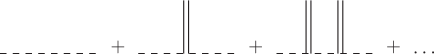
Figure 2: Dressed propagator $\langle\psi(1)\bar{\psi}(2)\rangle_{D}$. The vertices are $2(2h)^{2}(\Phi\bar{\Phi})\psi\bar{\psi}$.

Now, let us sum over the vertices $(2h)^{2}\bar{\Phi}\Phi\psi^{2}$ and $(2h)^{2}\bar{\Phi}\Phi\bar{\psi}^{2}$. The corresponding supergraphs again exhibit structures similar to Fig. 1 with only even number of vertices. However, it is worth to point out that we can insert an arbitrary number of vertices $(2h)^{2}\bar{\Phi}\Phi\psi\bar{\psi}$ into the propagators $\langle\psi(1)\bar{\psi}(2)\rangle$. Therefore, we should firstly introduce a "dressed" propagator. In this propagator, the summation over all vertices $(2h)^{2}\bar{\Phi}\Phi\psi\bar{\psi}$ is performed (see Fig. 2). As a result, this dressed propagator is equal to

$$\langle\psi(1)\bar{\psi}(2)\rangle_{D} = \langle\psi(1)\bar{\psi}(2)\rangle+\int d^{4}\theta_{3}\langle\psi(1)\bar{\psi}(3)\rangle[(2h)^{2}\bar{\Phi}\Phi]_{3}\langle\psi(3)\bar{\psi}(2)\rangle+\int d^{4}\theta_{3}d^{4}\theta_{4}$$ (25)

$$\times \langle\psi(1)\bar{\psi}(3)\rangle[(2h)^{2}\bar{\Phi}\Phi]_{3}\langle\psi(3)\bar{\psi}(4)\rangle[(2h)^{2}\bar{\Phi}\Phi]_{4}\langle\psi(4)\bar{\psi}(2)\rangle+\ldots\ .$$

By using (19), integrating by parts, and summing the resultant series, we arrive at

$$\langle\psi(1)\bar{\psi}(2)\rangle_{D}=\bigg{(}\frac{2\Pi_{1/2}}{1-2(2h)^{2}\bar{\Phi}\Phi}\bigg{)}_{1}\delta_{12}\ .$$ (26)

Afterwards, we can compute all the contributions by noting that each one-loop supergraph above is formed by $n$ vertices like those ones given by Fig. 3.

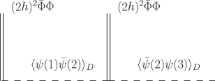
Figure 3: A typical vertex in one-loop supergraphs involving $(2h)^{2}\bar{\Phi}\Phi\psi^{2}$ and $(2h)^{2}\bar{\Phi}\Phi\bar{\psi}^{2}$.

Hence, the contribution of this vertex is given by

$$Q_{13} = \int d^{4}\theta_{2}[(2h)^{2}\bar{\Phi}\Phi]_{1}\Big{[}\Big{(}\frac{2\Pi_{1/2}}{1-2(2h)^{2}\bar{\Phi}\Phi}\Big{)}_{1}\delta_{12}\Big{]}[(2h)^{2}\bar{\Phi}\Phi]_{2}\Big{[}\Big{(}\frac{2\Pi_{1/2}}{1-2(2h)^{2}\bar{\Phi}\Phi}\Big{)}_{2}\delta_{23}\Big{]}$$ (27)

$$= \bigg{(}\frac{2(2h)^{2}\bar{\Phi}\Phi}{1-2(2h)^{2}\bar{\Phi}\Phi}\Pi_{1/2}\bigg{)}^{2}_{1}\delta_{13}\ .$$

It follows from the result above that the contribution of a supergraph formed by $n$ vertices is given by

$$I_{n} = \int d^{4}x\frac{1}{2n}\int d^{4}\theta_{1}d^{4}\theta_{3}\ldots d^{4}\theta_{2n-1}\int\frac{d^{4}p}{(2\pi)^{4}}Q_{13}Q_{35}\ldots Q_{2n-3,2n-1}Q_{2n-1,1}$$ (28)

$$= \int d^{4}x\frac{1}{2n}\int d^{4}\theta_{1}d^{4}\theta_{3}d^{4}\theta_{5}\ldots d^{4}\theta_{2n-1}\int\frac{d^{4}p}{(2\pi)^{4}}\Big{[}\bigg{(}\frac{2(2h)^{2}\bar{\Phi}\Phi}{1-2(2h)^{2}\bar{\Phi}\Phi}\Pi_{1/2}\bigg{)}^{2}_{1}\delta_{13}\Big{]}$$

$$\times \Big{[}\bigg{(}\frac{2(2h)^{2}\bar{\Phi}\Phi}{1-2(2h)^{2}\bar{\Phi}\Phi}\Pi_{1/2}\bigg{)}^{2}_{3}\delta_{35}\Big{]}\ldots\Big{[}\bigg{(}\frac{2(2h)^{2}\bar{\Phi}\Phi}{1-2(2h)^{2}\bar{\Phi}\Phi}\Pi_{1/2}\bigg{)}^{2}_{2n-1}\delta_{2n-1,1}\Big{]}$$

$$= \int d^{8}z\frac{1}{2n}\int\frac{d^{4}p}{(2\pi)^{4}}\bigg{(}\frac{2(2h)^{2}\bar{\Phi}\Phi}{1-2(2h)^{2}\bar{\Phi}\Phi}\bigg{)}^{2n}\Pi_{1/2}\delta_{\theta\theta^{\prime}}|_{\theta=\theta^{\prime}}\ .$$

By using $\Pi_{1/2}\delta_{\theta\theta^{\prime}}|_{\theta=\theta^{\prime}}=2/p^{2}$, we get the effective action

$$\Gamma^{(1)}_{1}=\sum_{n=1}^{\infty}I_{n}=-\int d^{8}z\int\frac{d^{4}p}{(2\pi)^{4}}\frac{1}{p^{2}}\ln\bigg{[}1-\bigg{(}\frac{2(2h)^{2}\bar{\Phi}\Phi}{1-2(2h)^{2}\bar{\Phi}\Phi}\bigg{)}^{2}\bigg{]}\ .$$ (29)

The integral over the momenta vanishes within the dimensional regularization scheme. Therefore,

$$\Gamma^{(1)}_{1}=0\ .$$ (30)

We will not calculate explicitly the one-loop supergraphs involving the gauge superfield propagators $\langle V(1)V(2)\rangle$ connecting the vertices $(2g)^{2}\bar{\Phi}\Phi V^{2}$, because the result is already known and described in SYM . Therefore, it is given by

$$\Gamma^{(1)}_{2}=-\int d^{8}z\int\frac{d^{4}p}{(2\pi)^{4}}\frac{1}{p^{2}}\ln\bigg{[}1+\frac{(2g)^{2}\bar{\Phi}\Phi}{p^{2}}\bigg{]}\ .$$ (31)

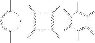
Figure 4: One-loop supergraphs composed by propagators $\langle\psi(1)\bar{\psi}(2)\rangle$ and $\langle V(1)V(2)\rangle$.

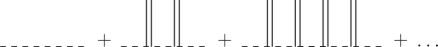
Figure 5: Dressed propagator $\langle\psi(1)\bar{\psi}(2)\rangle_{2D}$.

Finally, let us move on to the last type of one-loop supergraphs, which involve the propagators $\langle\psi(1)\bar{\psi}(2)\rangle$ and $\langle V(1)V(2)\rangle$ in the internal lines connecting the vertices $MV\psi$ and $MV\bar{\psi}$ (see Fig. 4). As before, we can insert an arbitrary number of vertices $(2h)^{2}\bar{\Phi}\Phi\psi\bar{\psi}$ into the propagators $\langle\psi(1)\bar{\psi}(2)\rangle$. Moreover, we can also insert an arbitrary number of pairs of the vertices $(2h)^{2}\bar{\Phi}\Phi\psi^{2}$ and $(2h)^{2}\bar{\Phi}\Phi\bar{\psi}^{2}$ into $\langle\psi(1)\bar{\psi}(2)\rangle$. Since $\langle\psi(1)\bar{\psi}(2)\rangle$ has already been dressed by $(2h)^{2}\bar{\Phi}\Phi\psi\bar{\psi}$ in (25-26), it follows that the desired dressed propagator $\langle\psi(1)\bar{\psi}(2)\rangle_{2D}$ is equal to the summation over all pairs of the vertices $(2h)^{2}\bar{\Phi}\Phi\psi^{2}$ and $(2h)^{2}\bar{\Phi}\Phi\bar{\psi}^{2}$ into $\langle\psi(1)\bar{\psi}(2)\rangle_{D}$ (see Fig. 5). Therefore, we get

$$\langle\psi(1)\bar{\psi}(2)\rangle_{2D} = \langle\psi(1)\bar{\psi}(2)\rangle_{D}+\int d^{4}\theta_{3}d^{4}\theta_{4}\langle\psi(1)\bar{\psi}(3)\rangle_{D}[(2h)^{2}\bar{\Phi}\Phi]_{3}\langle\bar{\psi}(3)\psi(4)\rangle_{D}$$ (32)

$$\times [(2h)^{2}\bar{\Phi}\Phi]_{4}\langle\psi(4)\bar{\psi}(2)\rangle_{D}+\int d^{4}\theta_{3}d^{4}\theta_{4}d^{4}\theta_{5}d^{4}\theta_{6}\langle\psi(1)\bar{\psi}(3)\rangle_{D}[(2h)^{2}\bar{\Phi}\Phi]_{3}$$

$$\times \langle\bar{\psi}(3)\psi(4)\rangle_{D}[(2h)^{2}\bar{\Phi}\Phi]_{4}\langle\psi(4)\bar{\psi}(5)\rangle_{D}[(2h)^{2}\bar{\Phi}\Phi]_{5}\langle\bar{\psi}(5)\psi(6)\rangle_{D}$$

$$\times [(2h)^{2}\bar{\Phi}\Phi]_{6}\langle\psi(6)\bar{\psi}(2)\rangle_{D}+\ldots\ .$$

After some algebraic work, we find

$$\langle\psi(1)\bar{\psi}(2)\rangle_{2D}=(2f(\bar{\Phi}\Phi)\Pi_{1/2})_{1}\delta_{12}\ ,\ \textrm{where}\ f(\bar{\Phi}\Phi)\equiv\frac{1}{1-4(2h)^{2}\bar{\Phi}\Phi}\ .$$ (33)

Additionally, we can also insert an arbitrary number of vertices $(2g)^{2}\bar{\Phi}\Phi V^{2}$ into the propagators $\langle V(1)V(2)\rangle$. In this case, the dressed propagator $\langle V(1)V(2)\rangle_{D}$ is already known in the literature and it is given by Our

$$\langle V(1)V(2)\rangle_{D}=\bigg{(}\frac{-\Pi_{1/2}}{p^{2}+(2g)^{2}\bar{\Phi}\Phi}\bigg{)}_{1}\delta_{12}\ .$$ (34)

As before, we can compute all the contributions by noting that each supergraph above (Fig. 4) is formed by $n$ fragments, like those depicted in Fig. 6. This fragment yields the contribution

$$R_{13} = \int d^{4}\theta_{2}(M)_{1}\Big{[}\Big{(}\frac{-\Pi_{1/2}}{p^{2}+(2g)^{2}\bar{\Phi}\Phi}\Big{)}_{1}\delta_{12}\Big{]}(M)_{2}\Big{[}(2f\Pi_{1/2})_{2}\delta_{23}\Big{]}$$ (35)

$$= \bigg{(}\frac{-2fM^{2}\Pi_{1/2}}{p^{2}+(2g)^{2}\bar{\Phi}\Phi}\bigg{)}_{1}\delta_{13}\ .$$

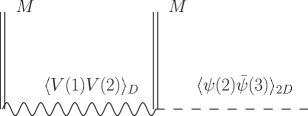
Figure 6: A typical vertex in one-loop supergraphs involving $MV\psi$ and $MV\bar{\psi}$.

It follows from the result above that the contribution of a supergraph formed by $n$ subgraphs is given by

$$J_{n} = \int d^{4}x\frac{1}{2n}\int d^{4}\theta_{1}d^{4}\theta_{3}\ldots d^{4}\theta_{2n-1}\int\frac{d^{4}p}{(2\pi)^{4}}R_{13}R_{35}\ldots R_{2n-3,2n-1}R_{2n-1,1}$$ (36)

$$= \int d^{4}x\frac{1}{2n}\int d^{4}\theta_{1}d^{4}\theta_{3}d^{4}\theta_{5}\ldots d^{4}\theta_{2n-1}\int\frac{d^{4}p}{(2\pi)^{4}}\Big{[}\bigg{(}\frac{-2fM^{2}\Pi_{1/2}}{p^{2}+(2g)^{2}\bar{\Phi}\Phi}\bigg{)}_{1}\delta_{13}\Big{]}$$

$$\times \Big{[}\bigg{(}\frac{-2fM^{2}\Pi_{1/2}}{p^{2}+(2g)^{2}\bar{\Phi}\Phi}\bigg{)}_{3}\delta_{35}\Big{]}\ldots\Big{[}\bigg{(}\frac{-2fM^{2}\Pi_{1/2}}{p^{2}+(2g)^{2}\bar{\Phi}\Phi}\bigg{)}_{2n-1}\delta_{2n-1,1}\Big{]}$$

$$= \int d^{8}z\frac{1}{2n}\int\frac{d^{4}p}{(2\pi)^{4}}\bigg{(}\frac{-2fM^{2}}{p^{2}+(2g)^{2}\bar{\Phi}\Phi}\bigg{)}^{n}\Pi_{1/2}\delta_{\theta\theta^{\prime}}|_{\theta=\theta^{\prime}}\ .$$

Again, by using $\Pi_{1/2}\delta_{\theta\theta^{\prime}}|_{\theta=\theta^{\prime}}=2/p^{2}$, we get the effective action

$$\Gamma^{(1)}_{3}=\sum_{n=0}^{\infty}J_{n}=-\int d^{8}z\int\frac{d^{4}p}{(2\pi)^{4}}\frac{1}{p^{2}}\ln\bigg{[}1+\frac{2fM^{2}}{p^{2}+(2g)^{2}\bar{\Phi}\Phi}\bigg{]}\ .$$ (37)

By summing (30), (31), and (37) we obtain the total one-loop effective action

$$\Gamma^{(1)}[\bar{\Phi},\Phi]=-\int d^{8}z\int\frac{d^{4}p}{(2\pi)^{4}}\frac{1}{p^{2}}\ln\big{[}p^{2}+(2g)^{2}\bar{\Phi}\Phi+2fM^{2}\big{]}\ .$$ (38)

Substituting the explicit form for $M$ and $f$, we arrive to the following result for the KEP:

$$K^{(1)}(\bar{\Phi},\Phi)=-\int\frac{d^{4}p}{(2\pi)^{4}}\frac{1}{p^{2}}\ln\big{[}p^{2}+\frac{1}{2-8(2h)^{2}\bar{\Phi}\Phi}(m-8gh\bar{\Phi}\Phi)^{2}+(2g)^{2}\bar{\Phi}\Phi\big{]}\ .$$ (39)

The integral above is well-known and can be computed by using the dimensional regularization. Finally, in the limit $\omega\rightarrow 2$ we find

$$K^{(1)}(\bar{\Phi},\Phi)=K_{div}^{(1)}(\bar{\Phi},\Phi)+K_{fin}^{(1)}(\bar{\Phi},\Phi)\ ,$$ (40)

where

$$K_{div}^{(1)}(\bar{\Phi},\Phi) = \frac{1}{16\pi^{2}(2-\omega)}\Big{[}\frac{1}{2-8(2h)^{2}\bar{\Phi}\Phi}(m-8gh\bar{\Phi}\Phi)^{2}+(2g)^{2}\bar{\Phi}\Phi\Big{]}\ ,$$ (41)

$$K_{fin}^{(1)}(\bar{\Phi},\Phi) = -\frac{1}{16\pi^{2}}\Big{[}\frac{1}{2-8(2h)^{2}\bar{\Phi}\Phi}(m-8gh\bar{\Phi}\Phi)^{2}+(2g)^{2}\bar{\Phi}\Phi\Big{]}$$ (42)

$$\times \ln\frac{1}{\mu^{2}}\Big{[}\frac{1}{2-8(2h)^{2}\bar{\Phi}\Phi}(m-8gh\bar{\Phi}\Phi)^{2}+(2g)^{2}\bar{\Phi}\Phi\Big{]}\ ,$$

and $\mu$ is an arbitrary scale required on dimensional grounds.

Notice that the one-loop KEP (40-42) is divergent. Moreover, we notice that the divergent part (41) is given by an infinite power series in $\bar{\Phi}\Phi$. Therefore, the theory under consideration is non-renormalizable and it must be interpreted as an effective field theory below some energy scale chosen on the basis of phenomenological considerations Bur .

In particular, let us take $h=0$ in (40). This choice corresponds to a minimal coupling between the gauge scalar superfield and the matter chiral superfields [see (10)]. Therefore,

$$K_{div}^{(1)}(\bar{\Phi},\Phi) = \frac{(2g)^{2}\bar{\Phi}\Phi}{16\pi^{2}(2-\omega)}\ ,$$ (43)

$$K_{fin}^{(1)}(\bar{\Phi},\Phi) = -\frac{1}{32\pi^{2}}\big{[}m^{2}+2(2g)^{2}\bar{\Phi}\Phi\big{]}\ln\frac{1}{2\mu^{2}}\big{[}m^{2}+2(2g)^{2}\bar{\Phi}\Phi\big{]}\ .$$ (44)

In this case, we notice that the divergent term (43) is proportional to $\bar{\Phi}\Phi$. Therefore, in order to remove divergences, we can insert a similar one-loop counterterm as the one used in the SQED. Moreover, if we take the massless case in (43-44), we recover the one-loop KEP for the usual SQED SYM .

IV Summary

We formulated a new theory involving coupling of three superfields of different natures: a chiral spinor gauge superfield originally introduced in Siegel together with the usual real scalar gauge superfield and the chiral scalar matter superfield. For this theory, we developed a superfield procedure for calculating the one-loop effective potential which we successfully found. The procedure does not essentially differ from the usual supergauge theories SYM with the rather similar structure of the one-loop contribution. The fact that the new theory is non-renormalizable is not unexpected since many non-polynomial supersymmetric theories are non-renormalizable GC ; Brignole . We expect that this theory, besides of the classical studies in the cosmic string context, can be used as an ingredient of possible phenomenologically interesting supersymmetric gauge theories involving several gauge (super)fields with some of them being massive.

Acknowledgments. This work was partially supported by Conselho Nacional de Desenvolvimento Científico e Tecnológico (CNPq). The work by A. Yu. P. has been partially supported by the CNPq project No. 303438/2012-6.

References

(1) S. J. Gates, M. T. Grisaru, M. Rocek, W. Siegel. Superspace or One Thousand and One Lessons in
Supersymmetry. Benjamin/Cummings, (1983), hep-th/0108200.
(2) I. L. Buchbinder and S. M. Kuzenko, Ideas and Methods of Supersymmetry and Supergravity. IOP Publishing, Bristol and Philadelphia, (1998).
(3) A. Yu. Petrov, “Quantum superfield supersymmetry”, hep-th/0106094.
(4) W. Siegel, Phys. Lett. B85, 333 (1979).
(5) C. N. Ferreira, J. A. Helayël-Neto, M. B. D. S. M. Porto, Nucl. Phys. B620, 181 (2002).
(6) J. Louis, J. Swiebodzinski, Eur. Phys. J. C51, 731 (2007), hep-th/0702211.
(7) I. L. Buchbinder, S. M. Kuzenko, J. V. Yarevskaya,
Nucl. Phys. B411, 665 (1994).
(8)I. L. Buchbinder, S. M. Kuzenko,
A. Yu. Petrov, Phys. Lett. B321, 372 (1994); Phys. At. Nucl. 59, 148 (1996).
(9) I. L. Buchbinder, A. Yu. Petrov, Phys. Lett. B461, 209
(1999), hep-th/9905062; I. L. Buchbinder, M. Cvetic, A. Yu. Petrov,
Mod. Phys. Lett. A15, 783 (2000), hep-th/9903243; Nucl. Phys. B571,
358 (2000),
hep-th/9906141.
(10) B. de Wit, M. Grisaru, M. Rocek, Phys. Lett. B374, 297
(1996), hep-th/9601115; M. Grisaru, M. Rocek, R. von Unge,
Phys. Lett. B383, 415 (1996), hep-th/9605149;
A. De Giovanni, M. Grisaru, M. Rocek, R. von
Unge, D. Zanon, Phys. Lett. B409, 251 (1997),
hep-th/9706013.
(11) H. R. Christiansen, M. S. Cunha, J. A. Helayël-Neto, L. R. U. Manssur, A. L. M. A. Nogueira, Int. J. Mod. Phys. A14, 147 (1999).
(12) R. Jackiw. D9, 1686 (1974);
I. L. Buchbinder, S. D. Odintsov, I. L. Shapiro. Effective
action in quantum gravity. IOP Publishing, Bristol and Philadelphia,
(1992).
(13) S. Coleman, Aspects of Symmetry, Cambridge Univ. Press, (1985).
(14) F. S. Gama, M. Gomes, J. R. Nascimento, A. Yu. Petrov, A. J. da Silva, Phys. Rev. D84, 045001 (2011), arXiv: 1101.0724; F. S. Gama, M. Gomes, J. R. Nascimento, A. Yu. Petrov, A. J. da Silva, Phys.Rev. D89 (2014) 085018, arXiv: 1401.6839.
(15) C. P. Burgess, Ann. Rev. Nucl. Part. Sci. 57, 329 (2007), hep-th/0701053.
(16) A. Brignole, Nucl. Phys. B579, 101 (2000), hep-th/0001121.