Quantization of the conformal arclength functional on space curves

Abstract.

By a conformal string in Euclidean space is meant a closed critical curve with non-constant conformal curvatures of the conformal arclength functional. We prove that (1) the set of conformal classes of conformal strings is in 1-1 correspondence with the rational points of the complex domain $\{q\in\mathbb{C}\,:\,{1}/{2}<{\rm Re}\,q<{1}/{\sqrt{2}},\,\,{\rm Im}\,q>0,\,\,|q|<{1}/{\sqrt{2}}\}$ and (2) any conformal class has a model conformal string, called symmetrical configuration, which is determined by three phenomenological invariants: the order of its symmetry group and its linking numbers with the two conformal circles representing the rotational axes of the symmetry group. This amounts to the quantization of closed trajectories of the contact dynamical system associated to the conformal arclength functional via Griffiths’ formalism of the calculus of variations.

Introduction

The Möbius geometry of space curves was mainly developed in the first half of the past century [9, 21, 37, 38] and later taken up starting from the early 1980’s [4, 19, 35, 36]. Further developments of the subject as an instance of the conformal geometry of submanifolds can be found in [2] and the literature therein. The subject has also received much attention for its many fields of application, including the theory of integrable systems [5, 8], the topology and Möbius energy of knots [1, 11, 18], and the geometric approach to shape analysis and medical imaging [34].

Let $\gamma\subset\mathbb{R}^{n}$, $n\geq 3$, be a smooth curve parametrized by arclength $s$. The conformal arclength parameter $\zeta$ of $\gamma$ is defined (up to a constant) by

(0.1) $$d\zeta=\left(\langle\dddot{\gamma},\dddot{\gamma}\rangle-\langle\ddot{\gamma},\ddot{\gamma}\rangle^{2}\right)^{\frac{1}{4}}ds=:\eta_{\gamma},$$

where $\langle\,,\rangle$ is the standard scalar product on $\mathbb{R}^{n}$. The 1-form $\eta_{\gamma}$, the infinitesimal conformal arclength of $\gamma$, is conformally invariant. If ${\eta_{\gamma}}{|_{s}}\neq 0$, for each $s$, the curve is called generic. The conformal arclength $\zeta$ gives a conformally invariant parametrization of a generic curve. We consider the conformally invariant variational problem on generic curves defined by the conformal arclength functional

(0.2) $$\mathcal{L}[\gamma]=\int_{\gamma}\eta_{\gamma}.$$

This variational problem was studied in [26] for $n=3$ and more recently in [22] for higher dimensions. Accordingly, the critical curves can be found by quadratures and explicit parametrizations are given in terms of elliptic functions and integrals. In this paper we address the question of existence and properties of closed critical curves for the functional $\mathcal{L}$. Actually, it suffices to consider the 3-dimensional case only, since from the results in [22] we can see that any closed critical curve in $\mathbb{R}^{n}$ lies in some $\mathbb{R}^{3}\subset\mathbb{R}^{n}$, up to a conformal transformation. It is known that a generic space curve is determined, up to conformal transformations, by the conformal arclength and two conformal curvatures (cf. Section 1). As for a closed critical curve with constant conformal curvatures, one can see that it is conformally equivalent to a closed rhumb line (loxodrome) of a torus of revolution (cf. Example 1).

The purpose of this paper is to study the class of closed critical curves with non-constant conformal curvatures, for brevity called conformal strings. We begin by describing our three main results. If $\gamma$, $\widetilde{\gamma}:\mathbb{R}\to\mathbb{R}^{3}$ are two curves and $[\gamma]$, $[\widetilde{\gamma}]$ denote their trajectories, then $\gamma$ and $\widetilde{\gamma}$ are said Möbius (conformally) equivalent if there is an element $A$ of the Möbius group $G$ of $\mathbb{R}^{3}$, such that $A\cdot[\gamma]=[\widetilde{\gamma}]$. By a conformal symmetry of a curve $\gamma$ is meant an element $A\in G$, such that $A\cdot[\gamma]=[\gamma]$. The set of all symmetries of $\gamma$ is a subgroup $G_{\gamma}$ of $G$. The symmetry group of a closed curve with non-constant conformal curvatures is finite and its cardinality is called the symmetry index of $\gamma$. Our first main result is the following.

Theorem A.

The Möbius classes of conformal strings are in 1-1 correspondence with the rational points of the complex domain

$$\Omega=\left\{q\in\mathbb{C}\,\,:\,\,\frac{1}{2}<{\rm Re}\,q<\frac{1}{\sqrt{2}},\,\,{\rm Im}\,q>0,\,\,|q|<\frac{1}{\sqrt{2}}\right\}.$$

The rational points of $\Omega$ are called the moduli of conformal strings.

Using this theorem and other technical results, we will prove that any Möbius class of strings is represented by a model string. This is our second main result.

Theorem B.

The conformal strings corresponding to a modulus $q\in\Omega$ are Möbius equivalent to a model string $\gamma_{q}=(x(t),y(t),z(t)):\mathbb{R}\to\mathbb{R}^{3}$,

(0.3) $$\begin{cases}x(t)=\frac{\sqrt{2}}{r(t)}\mu\sqrt{k(t)^{2}-\upsilon^{2}}\cos\Theta_{2}(t),\\ y(t)=\frac{\sqrt{2}}{r(t)}\mu\sqrt{k(t)^{2}-\upsilon^{2}}\sin\Theta_{2}(t),\\ z(t)=\frac{\sqrt{2}}{r(t)}\upsilon\sqrt{\mu^{2}-k(t)^{2}}\sin\Theta_{1}(t),\\ \end{cases}$$

called the symmetrical configuration of $q$. Here

$$k(t) =\left\{\!\!\!\begin{array}[]{lr}\sqrt{a}\operatorname{cn}\big{(}\sqrt{a-b}\,t,\frac{a}{a-b}\big{)},&b<0,\\ \sqrt{a}\operatorname{dn}\big{(}\sqrt{a}\,t,\frac{a-b}{a}\big{)},&b>0,\end{array}\right.$$

$$r(t) =\sqrt{\mu^{2}-\upsilon^{2}}k(t)+\upsilon\sqrt{\mu^{2}-k(t)^{2}}\cos\Theta_{1}(t),$$

where $\mu=\frac{1}{\sqrt{2}}\sqrt{a+b+\sqrt{4+(a-b)^{2}}}$, $\upsilon=\frac{1}{\sqrt{2}}\sqrt{a+b-\sqrt{4+(a-b)^{2}}}$,

$$\Theta_{1}(t)=\int_{0}^{t}\frac{\mu}{\mu^{2}-k(u)^{2}}du,\quad\Theta_{2}(t)=\int_{0}^{t}\frac{\upsilon}{\upsilon^{2}-k(u)^{2}}du,$$

and where $a$ and $b$ are real parameters, uniquely defined by $q$, such that $a>0$, $a>b$, $b\neq 0$, and $ab>1$.

The symmetry group of a symmetrical configuration has a special structure, which is described by the following.

Theorem C.

Let $\gamma_{q}:\mathbb{R}\to\mathbb{R}^{3}$ be the symmetrical configuration corresponding to the modulus $q=q_{1}+iq_{2}$, where $q_{1}=m_{1}/n_{1}$, $q_{2}=m_{2}/n_{2}$, and the pairs $(m_{1},n_{1})$, $(m_{2},n_{2})$ are coprime integers. Let $n$ be the least common multiple of $n_{1}$ and $n_{2}$, and consider the coprime integers $h_{1}=n/n_{1}$ and $h_{2}=n/n_{2}$. Then,

1. $n$ is the order of the symmetry group of $\gamma_{q}$;

2. $m_{1}h_{1}$ and $m_{2}h_{2}$ are the linking numbers of $\gamma_{q}$ with the Clifford circle

   $$\mathcal{C}=\left\{(x,y,0)\in\mathbb{R}^{3}:x^{2}+y^{2}=2\right\}$$

   and the $z$-axis, respectively.

An important consequence of the previous results is that the conformal shape of a string is uniquely determined by three phenomenological invariants: the order of its symmetry group and its linking numbers with the two axes of the symmetry group. The explicit construction of a string from the phenomenological invariants requires the inversion of the period map of $\mathcal{L}$ (cf. Section 2). In this respect, some numerical experiments carried out with the software Mathematica suggest that conformal strings are simple curves (cf. Section 6). However, a rigorous proof of this fact is still missing. Another interesting problem is to find an estimate for the asymptotic growth of $\varrho(n)$, the cardinality of the set of Möbius classes of strings with symmetry order $n$. Numerical experiments suggest a quadratic growth of $\varrho(n)$.

The theorems above have a conceptual explanation within the general scheme of Griffiths’ formalism of the calculus of variations [12, 13, 28, 29, 30, 31, 32]. Using Griffiths’ formalism, the momentum space of the variational problem can be identified with $Y=G_{+}\times\mathcal{A}$, where $G_{+}$ is the identity component of the Möbius group of $\mathbb{R}^{3}$ and $\mathcal{A}$ is a 3-dimensional submanifold of $\mathfrak{g}^{*}$, the dual of the Lie algebra of $G_{+}$. Moreover, the restriction $\xi\in\Omega^{1}(Y)$ of the Liouville form of $T^{*}(G_{+})$ defines an invariant contact structure on $Y$. By choosing a suitable set of coordinates on $\mathcal{A}$, say $p_{1}$, $p_{2}$ and $p_{3}$, the characteristic curves of the contact form are given by

$$t\in\mathbb{R}\mapsto(\mathrm{F}(t),p_{1}(t),p_{2}(t),p_{3}(t))\in Y,$$

where $\mathrm{F}$ is the canonical lift of a stationary curve $\gamma$, $p_{1}$ and $p_{2}$ are the conformal curvatures, and $p_{3}=p_{1}^{\prime}$. From a theoretical point of view, the study of the variational problem is equivalent to that of the dynamical system defined by the characteristic vector field of the contact form $\xi$. One can easily see that the contact momentum map is given by

$$J:(\mathrm{F},p)\in Y\mapsto\mathrm{Ad}^{*}(F)(\xi|_{(\mathrm{F},p)})\in\mathfrak{g}^{*}.$$

(For the construction of the momentum map in contact geometry, see for instance [33].) Moreover, the action of $G_{+}$ on $Y$ is Hamiltonian and coisotropic, and the characteristic vector field is collective completely integrable [10, 14, 17]. Consequently, the flow can be linearized on the fibers of the momentum map and its trajectories can be found by quadratures (see [12] for a general description of the integration procedure). Theorems A and C say that the contact dynamical system is quantizable, at least in the sense of “the old quantum theory” (Bohr’s atom theory) [24], and that the quantum numbers of the closed (quantizable) trajectories have a precise geometric meaning.

The paper is organized as follows. Section 1 collects some basic facts about the conformal geometry of space curves. Section 2 recalls the Euler–Lagrange equations of the variational problem and discusses the example of closed critical curves with constant conformal curvatures. Then, after introducing the natural parameters of a critical curve with non-constant periodic conformal curvatures, the period map of the functional $\mathcal{L}$ is defined, and conformal strings are characterized in terms of the natural parameters, via the period map. Section 3 deals with a technical result about the period map, from which Theorem A follows directly. Section 4 proves Theorem B, while Section 5 proves Theorem C. Section 6 discusses some examples.

Numerical and symbolic computations, as well as graphics, are made with the software Mathematica. As basic references for the theory of elliptic functions and integrals we use the monographs [3, 20] (see also [39]). For the few notions of knot theory used in the paper we refer to [23]. A general reference for Möbius geometry is [15], to which we refer for an updated list of modern and classical references to the subject (see also [16]). The main results of the paper were previously announced in [27].

(Added in proof) Since acceptance of the manuscript, the paper [7] has appeared, which studies the local and global conformal invariants of timelike curves in the (1+2)-Einstein universe and addresses the question of existence and properties of closed trajectories for the conformal strain functional.

Acknowledgments

The authors would like to thank the referees for their valuable comments and suggestions.

1. Preliminaries

1.1. The conformal group

Let $\mathbb{R}^{4,1}$ denote $\mathbb{R}^{5}$ with the Lorentz scalar product

(1.1) $$(v,w)=-(v^{0}w^{4}+v^{4}w^{0})+\sum_{j=1}^{3}v^{j}w^{j}=\sum_{a,b=0}^{4}g_{ab}v^{a}w^{b},\quad g_{ab}=g_{ba},$$

where $v=(v^{0},\dots,v^{4})$, and with the space and time orientations defined, respectively, by the volume form $dv^{0}\wedge\cdots\wedge dv^{4}$ and the positive light cone

(1.2) $$\mathcal{L}_{+}=\{v\in\mathbb{R}^{4,1}\,:\,(v,v)=0,\,v^{0}+v^{4}>0\}.$$

The Möbius space $\mathcal{M}_{3}$ is the projectivization of $\mathcal{L}_{+}$, endowed with the oriented conformal structure induced by the scalar product and the space and time orientations. If $(e_{0},\dots,e_{4})$ is the standard basis of $\mathbb{R}^{4,1}$, the map

(1.3) $$\mathcal{J}:x=(x^{1},x^{2},x^{3})\in\mathbb{R}^{3}\mapsto\left[\frac{\langle x,x\rangle}{2}e_{0}+\sum_{j=1}^{3}x^{j}e_{j}+e_{4}\right]\in\mathcal{M}_{3}.$$

is an orientation-preserving conformal diffeomorphism of $\mathbb{R}^{3}$ onto the Möbius space minus the point $P_{\infty}=[e_{0}]$. The inverse of $\mathcal{J}$ is the conformal projection

(1.4) $$\mathcal{P}:\left[\sum_{a=0}^{4}v^{a}e_{a}\right]\in\mathcal{M}_{3}\setminus\{P_{\infty}\}\mapsto\frac{1}{v^{4}}(v^{1},v^{2},v^{3})\in\mathbb{R}^{3}.$$

The Möbius group $G$ consists of all pseudo-orthogonal transformations preserving the volume form. It is a 10-dimensional Lie group with two connected components. The first component is the subgroup $G_{+}$ consisting of all $\mathrm{F}\in G$ preserving the positive light cone and the second one consists of all $\mathrm{F}\in G$ switching the positive light cone with the negative one. The group $G$ acts effectively and transitively on the left of $\mathcal{M}_{3}$ preserving the conformal structure. The classical Liouville theorem [6] asserts that every conformal automorphism of $\mathcal{M}_{3}$ is induced by a unique element of $G$. Consequently, the Möbius group can be viewed as the pseudo-group of all conformal transformations of Euclidean 3-space. The orientation-preserving conformal transformations are induced by the elements of $G_{+}$, while the conformal transformations induced the elements of $G_{-}$ are orientation-reversing. For each $\mathrm{F}\in G_{+}$, we denote by $\mathrm{F}_{0},\dots,\mathrm{F}_{4}$ its column vectors. Then, $(\mathrm{F}_{0},\dots,\mathrm{F}_{4})$ is a positive light cone basis of $\mathbb{R}^{4,1}$, that is a positive-oriented basis such that

$$(\mathrm{F}_{a},\mathrm{F}_{b})=g_{ab},\quad\mathrm{F}_{0},\mathrm{F}_{4}\in\mathcal{L}_{+},\quad a,b=0,\dots,4.$$

Conversely, if $(\mathrm{F}_{0},\dots,\mathrm{F}_{4})$ is a positive light-cone basis, then the matrix $\mathrm{F}$ with column vectors $\mathrm{F}_{0},\dots,\mathrm{F}_{4}$ i s an element of $G_{+}$. The Lie algebra of $G$ consists of all skew-adjoint matrices of the scalar product (1.1), that is

$$\mathfrak{g}=\left\{\mathrm{X}\in\mathfrak{gl}(5,\mathbb{R})\,:\,^{t}\mathrm{X}g+g\mathrm{X}=0\right\},$$

where $g=(g_{ab})$. The maximal compact abelian subgroups of $G$ are conjugate to the 2-dimensional torus

(1.5) $$T=\left\{R(\phi_{1},\phi_{2})\,:\,\phi_{1},\phi_{2}\in[0,2\pi)\right\}\cong SO(2)\times SO(2),$$

where

(1.6) $$R(\phi_{1},\phi_{2})=\left(\begin{smallmatrix}\frac{1+\cos\phi_{2}}{2}&0&0&-\frac{\sin\phi_{2}}{\sqrt{2}}&\frac{1-\cos\phi_{2}}{2}\\ 0&\cos\phi_{1}&-\sin\phi_{1}&0&0\\ 0&\sin\phi_{1}&\cos\phi_{1}&0&0\\ \frac{\sin\phi_{2}}{\sqrt{2}}&0&0&\cos\phi_{2}&-\frac{\sin\phi_{2}}{\sqrt{2}}\\ \frac{1-\cos\phi_{2}}{2}&0&0&\frac{\sin\phi_{2}}{\sqrt{2}}&\frac{1+\cos\phi_{2}}{2}\\ \end{smallmatrix}\right).$$

Note that $R(\phi_{1},\phi_{2})$ is the composition of the Euclidean rotation of angle $\phi_{1}$ around the $z$-axis with the toroidal rotation of angle $\phi_{2}$ around the Clifford circle $\mathcal{C}=\{(x,y,0):x^{2}+y^{2}=2\}$. The $z$-axis and the Clifford circle are the rotational axes of $T$. The rotational axes of any other maximal torus $\mathrm{F}T\mathrm{F}^{-1}$ are the images under $\mathrm{F}$ of the axes of $T$.

1.2. Möbius geometry of space curves

Let $\gamma:I\subset\mathbb{R}\to\mathbb{R}^{3}$ be a smooth curve parametrized by arclength $s$, $I$ an open interval. Points where the infinitesimal conformal arclength $\eta_{\gamma}$ (cf. (0.1)) vanishes are called vertices of $\gamma$ (cf. [4, 19]). Generic curves, i.e., without vertices, can be parametrized by the conformal arclength parameter $\zeta$, defined (up to a constant) by $d\zeta=\eta_{\gamma}$. If such a conformal parametrization is defined for every $\zeta\in\mathbb{R}$, the curve is said complete. A frame field along $\gamma$ is a smooth map $\mathrm{F}:I\to G_{+}$, such that $\mathcal{P}\circ\mathrm{F}_{4}=\gamma$. We have the following.

Proposition 1.1 (cf. [4, 9, 22, 26, 36]).

For any oriented generic curve $\gamma:I\to\mathbb{R}^{3}$, there is a unique frame field $\mathrm{F}:I\to G_{+}$ along $\gamma$, the Vessiot frame, such that

(1.7) $$\mathrm{F}^{-1}d\mathrm{F}=\left(\begin{smallmatrix}0&1&0&0&0\\ k_{2}&0&0&0&1\\ 1&0&0&k_{1}&0\\ 0&0&-k_{1}&0&0\\ 0&k_{2}&1&0&0\\ \end{smallmatrix}\right)\eta_{\gamma},$$

where $k_{1}$, $k_{2}$ are smooth functions, called the conformal curvatures. We call $\Gamma=\mathrm{F}_{4}:I\to\mathcal{L}_{+}$ the canonical null lift of $\gamma$.

Remark 1.

If $\gamma$ is biregular and $T=\dot{\gamma}$, $N$, $B$ is its Frenet frame, with Frenet–Serret equations $\dot{T}=\kappa N$, $\dot{N}=-\kappa T+\tau B$, $\dot{B}=-\tau N$, we have ${\dddot{\gamma}}=-\kappa^{2}T+\dot{\kappa}N+\kappa\tau B$ and then $\eta_{\gamma}=\sqrt[4]{\dot{\kappa}^{2}+\kappa^{2}\tau^{2}}\,ds$ (cf. [36, 37]). The conformal curvatures take the form

(1.8) $$k_{1}=r^{5}\left(\kappa^{2}\tau^{3}+\kappa\dot{\kappa}\dot{\tau}+\tau(2\dot{\kappa}^{2}-\kappa\ddot{\kappa})\right),\quad k_{2}=\frac{1}{2}\left(\dot{r}^{2}-2r\ddot{r}-r^{2}\kappa^{2}\right),$$

where $r=(\dot{\kappa}^{2}+\kappa^{2}\tau^{2})^{-1/4}$ (cf. [36]). For a geometric description of vertices and the conformal arclength via the osculating circles of $\gamma$ we refer to [19, 25].

Remark 2.

The construction of $\mathrm{F}$ is explicit and only involves derivatives and simplification of $\mathrm{F}^{-1}d\mathrm{F}$ by linear relations on entries. If $\gamma:\mathbb{R}\to\mathbb{R}^{3}$ is a periodic parametrization of a closed curve, $\mathrm{F}$ is a periodic $G_{+}$-valued map. The value of $\mathrm{F}$ at $t\in I$ depends on the fourth order jet of $\gamma$ at $t$. If $\eta_{\gamma}=d\zeta$, any solution of the linear system (1.7) is the Vessiot frame of the conformal parametrization $\gamma=\mathcal{P}\circ[\mathrm{F}_{4}]$ of a generic curve with curvatures $k_{1}$ and $k_{2}$. If $\mathrm{F}$, $\widetilde{\mathrm{F}}:\mathbb{R}\to G_{+}$ are two solutions of (1.7), with initial conditions in $G_{+}$, there is a unique $A\in G_{+}$, such that $\widetilde{\mathrm{F}}=A\mathrm{F}$. This shows that the conformal curvatures determine the curve, up to an orientation-preserving conformal transformation.

A curve $\gamma:\mathbb{R}\to\mathbb{R}^{3}$ is called chiral if its symmetry group $G_{\gamma}$ is contained in $G_{+}$.

Definition 1.1.

A generic curve $\gamma:\mathbb{R}\to\mathbb{R}^{3}$ parametrized by conformal arclength is said quasi-periodic if its conformal curvatures are non constant, periodic, with a common minimal period $\omega>0$; $\omega$ is called the conformal wavelength of $\gamma$.

The monodromy of a quasi-periodic curve is the element $M:=\mathrm{F}(\omega)\mathrm{F}(0)^{-1}\in G_{+}$. By construction, $M$ satisfies

(1.9) $$\mathrm{F}(t+p\omega)=M^{p}\mathrm{F}(t),\quad\forall t\in\mathbb{R},\quad\forall p\in\mathbb{Z}.$$

Therefore, $M$ generates a subgroup $\widehat{G}_{\gamma}\subset G_{\gamma}$, the monodromy group of $\gamma$. If $\gamma$ is closed, the integral of $\eta_{\gamma}$ along $\gamma$ is $n\omega$, where $n$ is the cardinality of $\widehat{G}_{\gamma}$.

If $A$ is an orientation-reversing conformal transformation, the conformal curvatures of $A\cdot\gamma$ are $-k_{1}$ and $k_{2}$, respectively. Thus, generic curves whose first curvature is nowhere vanishing are chiral. In this case, we assume that $\gamma$ has positive chirality (i.e., $k_{1}>0$). If $\gamma$ is a real-analytic curve with positive chirality, then $\widehat{G}_{\gamma}=G_{\gamma}$ and $\gamma$ is closed if and only if $M$ has finite order. Note that the symmetry index of a real-analytic closed curve with positive chirality coincides with the order of the monodromy.

2. Critical curves

2.1. The Euler-Lagrange equations

The critical curves of the functional $\mathcal{L}$ (0.2) are characterized by the Euler–Lagrange equations [26]

(2.1) $$k_{1}^{\prime\prime}=2k_{1}(C_{1}-k_{1}^{2}),\quad k_{2}=-\frac{3}{2}k_{1}^{2}+C_{1},$$

where $C_{1}$ is a constant of integration and $k_{1}^{\prime\prime}$ is the second order derivative of $k_{1}$ with respect to the conformal arclength $\zeta$.

Example 1 (Critical curves with constant conformal curvatures).

Let $\gamma$ be a critical curve with constant conformal curvatures. Then, either $k_{1}=0$ and $k_{2}\in\mathbb{R}$, or $k_{2}=-k_{1}^{2}/2$ and $k_{1}\in\mathbb{R}\setminus\{0\}$. In the second case, we may assume $k_{1}>0$. The class of curves with constant conformal curvatures was studied in [36]: they are equivalent to the rhumb lines of either a torus of revolution, or a round cone, or else a circular cylinder. Since we deal with curves without vertices, the meridians and the parallels must be excluded from the discussion. The rhumb lines of a round cone, which possibly can degenerate into the punctured plane, are helices over logarithmic spirals, while the rhumb lines of a circular cylinder are circular helices. All of them are not closed. From the viewpoint of the conformal geometry, any rotationally invariant torus is equivalent to a torus $\mathcal{T}_{r}$ generated by rotating around the $z$-axis the circle in the $xz$-plane with radius $(2-r^{2})/2r$ and center $((r^{2}+1)/2r,0,0)$, for some $r\in(0,\sqrt{2})$. The latter are the regular orbits of the action of the group $T$ (cf. (1.5)) on the Euclidean space. If

$$\begin{cases}x_{r}(\theta,\phi)=\frac{4r\cos\theta}{2+r^{2}+(2-r^{2})\cos\phi},\\ y_{r}(\theta,\phi)=\frac{4r\sin\theta}{2+r^{2}+(2-r^{2})\cos\phi},\\ z_{r}(\theta,\phi)=\frac{\sqrt{2}(r^{2}-2)\sin\phi}{2+r^{2}+(2-r^{2})\cos\phi}\end{cases}$$

are parametric equations of $\mathcal{T}_{r}$, its rhumb lines are

$$\alpha_{r,m,n}:t\in\mathbb{R}\mapsto(x_{r}(nt,mt),y_{r}(nt,mt),z_{r}(nt,mt))\in\mathbb{R}^{3},$$

where $m,n\in\mathbb{R}$ and $mn\neq 0,n\neq\pm m$. The conformal curvatures of $\alpha_{r,m,n}$ are

$$\begin{cases}k_{1}=-\frac{(2+r^{2})mn}{\sqrt[4]{8m^{2}n^{2}(m^{2}-n^{2})^{2}r^{2}(2-r^{2})^{2}}},\\ k_{2}=\frac{(8n^{4}r^{2}+m^{4}(r^{2}-2)^{2})\mid mn(m^{2}-n^{2})\mid}{4\sqrt{2}rm^{2}n^{2}(m^{2}-n^{2})(r^{2}-2)}.\end{cases}$$

They verify the inequality $2k_{1}^{2}k_{2}<-1$. Conversely, every curve with constant conformal curvatures that satisfies the above inequality is equivalent to a rhumb line of $\mathcal{T}_{r}$, for some $r\in(0,\sqrt{2})$. Possibly, $r$ can be computed in terms of the constants $k_{1}$ and $k_{2}$. From this it follows that, up to conformal transformations, the only closed critical curves with constant conformal curvatures are of the form $\alpha_{r(q),q,1}$, where $q$ is a positive rational number different from $1$ and

$$r(q)=\frac{\sqrt{2}}{q}\sqrt{2+q^{2}-2\sqrt{1+q^{2}}}.$$

The trajectory of $\alpha_{r(q),q,1}$ is a torus knot of type $(m,n)$, where $m,n$ are coprime integers such that $m/n=q$, see Figure 1.

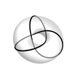
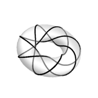
Figure 1. Closed critical curves with constant conformal curvatures and torus knots of type $(3,2)$ and $(7,3)$, respectively.

From now on we consider critical curves with non-constant conformal curvatures, parametrized by the conformal arclength parameter. Then, (2.1) implies

(2.2) $$(k_{1}^{\prime})^{2}+k_{1}^{4}-2C_{1}k_{1}^{2}=C_{2},$$

where $C_{2}$ is another constant of integration. This equation has non-constant periodic solutions if and only if the polynomial $P(t,C_{1},C_{2})=t^{2}-2C_{1}t-C_{2}$ has two distinct real roots, denoted by $a,b$ and ordered in such a way that $a>b$, with $a>0$ and $b\neq 0$. Then (2.1) can be rewritten in the form

(2.3) $$(k_{1}^{\prime})^{2}+(k_{1}^{2}-a)(k_{1}^{2}-b)=0,\quad k_{2}=-\frac{3}{2}k_{1}^{2}+\frac{a+b}{2}.$$

The general solution of (2.3) is given by

(2.4) $$k_{1}(t)=\epsilon_{1}k_{(a,b)}(\epsilon_{2}t+h),\quad k_{2}(t)=-\frac{3}{2}k_{1}(t)^{2}+\frac{a+b}{2},$$

where $\epsilon_{1},\epsilon_{2}=\pm 1$, $h$ is any real constant, and $k_{(a,b)}$ is the Jacobi elliptic function

(2.5) $$k_{(a,b)}(t)=\begin{cases}\sqrt{a}\operatorname{cn}\big{(}\sqrt{a-b}t,\frac{a}{a-b}\big{)},\quad b<0,\\ \sqrt{a}\operatorname{dn}\big{(}\sqrt{a}t,\frac{a-b}{a}\big{)},\quad\quad\,\,\,b>0.\end{cases}$$

By possibly reversing the orientation along the curve, acting with an orientation-reversing conformal transformation and shifting the independent variable, we can assume that $\epsilon_{1}=\epsilon_{2}=1$ and $h=0$. We have proved the following.

Proposition 2.1.

The Möbius classes of quasi-periodic critical curves are in 1-1 correspondence with the points $(a,b)$ of the planar region

(2.6) $$S=\left\{(a,b)\,:\,a>0,\,a>b,\,b\neq 0\right\}.$$

We call $a$ and $b$ the parameters of a quasi-periodic critical curve.

Remark 3.

The Möbius class of a critical curve with parameters $a$ and $b$ is represented by any conformal parametrization $\gamma:\mathbb{R}\to\mathbb{R}^{3}$ with curvatures

(2.7) $$k_{1}=k_{(a,b)},\quad k_{2}=-\frac{3}{2}k_{(a,b)}^{2}+\frac{a+b}{2}.$$

Note that the minimal period of $k_{(a,b)}$ is given by

(2.8) $$\omega_{(a,b)}=\begin{cases}{4K\left(a(a-b)^{-1}\right)}/{\sqrt{a-b}}\quad&b<0,\\ {2K\left(b^{-1}(a-b)\right)}/{\sqrt{a}}\quad&b>0,\end{cases}$$

where

(2.9) $$K(m)=\int_{0}^{\pi/2}\frac{1}{\sqrt{1-m\sin^{2}t}}dt$$

is the complete elliptic integral of the first kind.

2.2. Closure conditions

Let $\Sigma$ denote the open subset of $S\subset\mathbb{R}^{2}$ defined by

(2.10) $$\Sigma=\left\{(a,b)\in S\,:\,ab>1\right\}.$$

For every $(a,b)\in\Sigma$, let

(2.11) $$\mu(a,b) =\frac{1}{\sqrt{2}}\sqrt{a+b+\sqrt{4+(a-b)^{2}}},$$

$$\upsilon(a,b) =\frac{1}{\sqrt{2}}\sqrt{a+b-\sqrt{4+(a-b)^{2}}},$$

and define

(2.12) $$\Phi_{1}(a,b) :=\frac{1}{2\pi}\int_{0}^{\omega(a,b)}\frac{\mu(a,b)}{k_{(a,b)}(t)^{2}-\mu(a,b)^{2}}dt,$$

$$\Phi_{2}(a,b) :=\frac{1}{2\pi}\int_{0}^{\omega(a,b)}\frac{\upsilon(a,b)}{k_{(a,b)}(t)^{2}-\upsilon(a,b)^{2}}dt.$$

These integrals can be evaluated in term of the complete integral of the third kind (cf., for example, [39])

(2.13) $$\Pi(n,m)=\int_{0}^{\pi/2}\frac{dt}{(1-n\sin^{2}t)\sqrt{1-m\sin^{2}t}},\quad-1<n,m<1.$$

As a result, we have

(2.14) $$\Phi_{1}(a,b) =\frac{\mu(a,b)}{\pi\sqrt{a}(a-\mu(a,b)^{2})}\Pi\left(\frac{a-b}{a-\mu(a,b)^{2}},\frac{a-b}{a}\right),$$

$$\Phi_{2}(a,b) =\frac{\upsilon(a,b)}{\pi\sqrt{a}(a-\upsilon(a,b)^{2})}\Pi\left(\frac{a-b}{a-\upsilon(a,b)^{2}},\frac{a-b}{a}\right).$$

Definition 2.1.

We call $\Phi=(\Phi_{1},\Phi_{2}):\Sigma\to\mathbb{R}^{2}$ the period map of the conformal arclength functional. By construction, $\Phi$ is non constant and real analytic.

We are now in a position to state the following.

Theorem 2.2.

A quasi-periodic critical curve with parameters $a$ and $b$ is a conformal string if and only if $(a,b)\in\Sigma$ and $\Phi_{1}(a,b)$, $\Phi_{2}(a,b)\in\mathbb{Q}$.

For every $(a,b)\in S$, let $\gamma:\mathbb{R}\to\mathbb{R}^{3}$ be the conformal parametrization of a quasi-periodic critical curve with parameters $(a,b)\in S$, such that $\mathrm{F}(0)=\mathrm{Id}$, where $\mathrm{F}$ is the Vessiot frame along $\gamma$. The claim is that $\gamma$ is periodic if and only if $(a,b)\in\Sigma$ and $\Phi_{j}(a,b)\in\mathbb{Q}$, $j=1,2$. For brevity, let $k$ denote the first conformal curvature $k_{1}$, let $\mu$ and $\upsilon$ denote the constants $\mu(a,b)$, $\upsilon(a,b)$, respectively, and let $\omega$ denote the minimal period $\omega(a,b)$.

Lemma 2.3 (cf. [26]).

The canonical null lift $\Gamma:\mathbb{R}\to\mathcal{L}_{+}$ of $\gamma$ satisfies the linear system

(2.15) $$X^{\prime} =\left(\frac{k^{\prime}}{k}\mathrm{Id}-\frac{k^{2}-a-b}{k^{\prime 2}+1}\mathfrak{X}+\frac{k^{\prime}(k^{2}-a-b)}{k(k^{\prime 2}+1)}\mathfrak{X}^{2}\right.$$

$$\qquad\left.+\frac{1}{k^{\prime 2}+1}\mathfrak{X}^{3}-\frac{k^{\prime}}{k(k^{\prime 2}+1)}\mathfrak{X}^{4}\right)X,$$

with the initial condition $\Gamma(0)=e_{4}$, where

$$\mathfrak{X}=\left(\begin{smallmatrix}0&0&1&0&0\\ 1&0&0&\sqrt{a}&0\\ -b/2&0&0&0&1\\ 0&-\sqrt{a}&0&0&0\\ 0&1&-b/2&0&0\\ \end{smallmatrix}\right)\in\mathfrak{g}.$$

Using Lemma 2.3, an explicit integration of the critical curves was carried out in [26] (see also [22]). The proof of Theorem 2.2 is a direct consequence of this integration. According to the analysis carried out in [26], we are led to consider three cases, depending on whether $ab<1$, $ab=1$, or $ab>1$. It follows from [26] that the conformal parametrizations of a quasi-periodic critical curve with parameters $a$, $b$ can only be periodic if $ab>1$, in which case the following holds.

Lemma 2.4.

A quasi-periodic critical curve with $ab>1$ is closed if and only if $\Phi_{1}(a,b)$ and $\Phi_{2}(a,b)$ are rational numbers.

Proof of Lemma 2.4.

Assume that $a>0$, $a>b$, and $ab>1$. Then, the eigenvalues of $\mathfrak{X}$ are $\lambda_{0}=0$, $\lambda_{1,\pm}=\pm i\mu$, and $\lambda_{2,\pm}=\pm i\upsilon$. Choose $Y\in GL(5,\mathbb{C})$, such that

$$\hat{\mathfrak{X}}=Y^{-1}\mathfrak{X}Y=\left(\begin{smallmatrix}0&0&0&0&0\\ 0&i\mu&0&0&0\\ 0&0&-i\mu&0&0\\ 0&0&0&i\upsilon&0\\ 0&0&0&0&-i\upsilon\\ \end{smallmatrix}\right)$$

and consider the map $V=Y^{-1}\Gamma:\mathbb{R}\to\mathbb{C}^{5}$. From (2.15), it follows that the components $v_{0},\dots,v_{4}$ of $V$ satisfy

$$\begin{cases}v_{0}^{\prime}=\frac{k^{\prime}}{k}v_{0},\\ v^{\prime}_{1}=\left(\frac{k^{\prime}}{k}-i\frac{k^{2}-a-b}{k^{\prime 2}+1}\mu-\frac{k^{\prime}(k^{2}-a-b)}{k(k^{\prime 2}+1)}\mu^{2}-i\frac{1}{k^{\prime 2}+1}\mu^{3}+\frac{k^{\prime}}{k(k^{\prime 2}+1)}\mu^{4}\right)v_{1},\\ v^{\prime}_{2}=\left(\frac{k^{\prime}}{k}+i\frac{k^{2}-a-b}{k^{\prime 2}+1}\mu-\frac{k^{\prime}(k^{2}-a-b)}{k(k^{\prime 2}+1)}\mu^{2}+i\frac{1}{k^{\prime 2}+1}\mu^{3}+\frac{k^{\prime}}{k(k^{\prime 2}+1)}\mu^{4}\right)v_{2},\\ v^{\prime}_{3}=\left(\frac{k^{\prime}}{k}-i\frac{k^{2}-a-b}{k^{\prime 2}+1}\upsilon-\frac{k^{\prime}(k^{2}-a-b)}{k(k^{\prime 2}+1)}\upsilon^{2}-i\frac{1}{k^{\prime 2}+1}\upsilon^{3}+\frac{k^{\prime}}{k(k^{\prime 2}+1)}\upsilon^{4}\right)v_{3},\\ v^{\prime}_{4}=\left(\frac{k^{\prime}}{k}+i\frac{k^{2}-a-b}{k^{\prime 2}+1}\upsilon-\frac{k^{\prime}(k^{2}-a-b)}{k(k^{\prime 2}+1)}\upsilon^{2}+i\frac{1}{k^{\prime 2}+1}\upsilon^{3}+\frac{k^{\prime}}{k(k^{\prime 2}+1)}\upsilon^{4}\right)v_{4}.\end{cases}$$

Using $k^{\prime 2}+(k^{2}-a)(k^{2}-b)=0$, the above equations take the form

$$v^{\prime}_{1} =-\frac{kk^{\prime}+i\mu}{\mu^{2}-k^{2}}v_{1},\quad v_{2}^{\prime}=\frac{-kk^{\prime}+i\mu}{\mu^{2}-k^{2}}v_{2},$$

$$v_{3}^{\prime} =-\frac{kk^{\prime}+i\upsilon}{\upsilon^{2}-k^{2}}v_{3},\quad v_{4}^{\prime}=\frac{-kk^{\prime}+i\upsilon}{\upsilon^{2}-k^{2}}v_{4}.$$

Thus $v_{a}=p_{a}w_{a}$, where $p_{0},\dots,p_{4}\in\mathbb{C}$ and $w_{0},\dots,w_{4}$ are the complex-valued functions given by

$$w_{0} =k,\quad w_{1}=\sqrt{\mu^{2}-k^{2}}e^{i\int\frac{\mu}{\mu^{2}-k^{2}}dt},\quad w_{2}=\sqrt{\mu^{2}-k^{2}}e^{-i\int\frac{\mu}{\mu^{2}-k^{2}}dt},$$

$$w_{3} =\sqrt{\upsilon^{2}-k^{2}}e^{i\int\frac{\upsilon}{\upsilon^{2}-k^{2}}dt},\quad w_{4}=\sqrt{\upsilon^{2}-k^{2}}e^{-i\int\frac{\upsilon}{\upsilon^{2}-k^{2}}dt}.$$

Since $k$ is a non-constant periodic function with minimal period $\omega$, the functions $w_{0},\dots,w_{4}$ are periodic if and only if

$$\Phi_{1}=\frac{1}{2\pi}\int_{0}^{\omega}\frac{\mu}{k(t)^{2}-\mu^{2}}dt\in\mathbb{Q},\quad\Phi_{2}=\frac{1}{2\pi}\int_{0}^{\omega}\frac{\upsilon}{k(t)^{2}-\upsilon^{2}}dt\in\mathbb{Q},$$

which proves the lemma. ∎

This proves Theorem 2.2. As a corollary, we have the following.

Proposition 2.5.

The Möbius classes of conformal strings are in 1-1 correspondence with the elements of the countable set

$$\Sigma_{*}=\left\{(a,b)\in\mathbb{R}^{2}\,:\,a>0,\,a>b,\,ab>1,\,\Phi_{1}(a,b),\,\Phi_{2}(a,b)\in\mathbb{Q}\right\}.$$

This Proposition will be used in the proof of Theorem A.

3. The proof of Theorem A

Theorem A asserts that the Möbius classes of conformal strings are in one-to-one correspondence with the rational points of the complex domain

$$\Omega=\left\{q\in\mathbb{C}\,:\,{1}/{2}<{\rm Re}\,q<{1}/{\sqrt{2}},\,\,{\rm Im}\,q>0,\,\,|q|<{1}/{\sqrt{2}}\right\}.$$

The proof of Theorem A will follow from Proposition 2.5 and the next result about the period map $\Phi$ (cf. Definition 2.1).

Theorem 3.1.

The period map $\Phi=(\Phi_{1},\Phi_{2}):\Sigma\to\mathbb{R}^{2}$ is a real-analytic diffeomorphism onto the domain

$$\widetilde{\Omega}=\left\{(x,y)\in\mathbb{R}^{2}\,:\,-1/\sqrt{2}<x<-1/2,\,x^{2}+y^{2}<1/2,\,y>0\right\}.$$

The proof of Theorem 3.1 is based on a detailed study of the analytic properties of $\Phi$. This study is split into several technical results which will take up the remaining part of the section.

3.1. Preparatory material

Note that $\Phi_{1}$, $\Phi_{2}:\Sigma\to\mathbb{R}$, and hence the period map $\Phi=(\Phi_{1},\Phi_{2})$, extend analytically to the domain

$$\widetilde{\Sigma}=\left\{(a,b)\,:\,a>0,\,ab\geq 1\right\}.$$

Slightly abusing notation, we will retain the same letters for the extensions of $\Phi_{1}$ and $\Phi_{2}$ to $\widetilde{\Sigma}$. Let

(3.1) $$E:m\in[0,1)\mapsto\int_{0}^{\pi/2}\sqrt{1-m\sin^{2}t}dt\in\mathbb{R}$$

be the elliptic integral of the second kind. Then, $E(m)<K(m)$ and the ratio $E/K$ is a strictly decreasing function from $[0,1)$ onto $(0,1]$. The power series of $K$ and $E$ (cf. [20], p. 73, and [39]) are given by

(3.2) $$\begin{cases}K(m)=\frac{\pi}{2}\left(1+\frac{1}{4}m+\left(\frac{1\cdot 3}{2\cdot 4}\right)^{2}m^{2}+\left(\frac{1\cdot 3\cdot 5}{2\cdot 4\cdot 6}\right)^{2}m^{3}+\cdots\right),\\ E(m)=\frac{\pi}{2}\left(1-\frac{1}{4}m-\frac{1}{3}\left(\frac{1\cdot 3}{2\cdot 4}\right)^{2}m^{2}-\frac{1}{5}\left(\frac{1\cdot 3\cdot 5}{2\cdot 4\cdot 6}\right)^{2}m^{3}+\cdots\right).\end{cases}$$

We also recall the expressions of the derivatives of the complete elliptic integral of the third kind $\Pi$ given in (2.13) (cf. [20], §3.7-3.9, and [39]),

(3.3) $$\begin{cases}\partial_{n}\Pi|_{(n,m)}=\frac{nE(m)+(m-n)K(m)+(n^{2}-m)\Pi(n,m)}{2(m-n)(n-1)n},\\ \partial_{m}\Pi|_{(n,m)}=\frac{E(m)}{2(m-1)(n-m)}+\frac{\Pi(n,m)}{2(n-m)}.\end{cases}$$

3.2. The derivatives of $\Phi_{1}$ and $\Phi_{2}$

Using (2.14) and (3.3), we have

(3.4) $$\begin{cases}(\mathrm{i})&\partial_{a}\Phi_{1}|_{(a,b)}=\frac{X_{11}(a,b)E(\frac{a-b}{a})+Y_{11}(a,b)K(\frac{a-b}{b})}{Z_{11}(a,b)},\\ (\mathrm{ii})&\partial_{b}\Phi_{1}|_{(a,b)}=\frac{X_{21}(a,b)E(\frac{a-b}{a})+Y_{21}(a,b)K(\frac{a-b}{b})}{Z_{21}(a,b)},\\ (\mathrm{iii})&\partial_{a}\Phi_{2}|_{(a,b)}=\frac{X_{12}(a,b)E(\frac{a-b}{a})+Y_{12}(a,b)K(\frac{a-b}{b})}{Z_{12}(a,b)},\\ (\mathrm{iv})&\partial_{b}\Phi_{2}|_{(a,b)}=\frac{X_{22}(a,b)E(\frac{a-b}{a})+Y_{22}(a,b)K(\frac{a-b}{b})}{Z_{22}(a,b)},\\ \end{cases}$$

where the coefficients $X_{ij}(a,b)$, $Y_{ij}(a,b)$, and $Z_{ij}(a,b)$ are given by

$$\begin{cases}X_{11}(a,b)=\sqrt{2}\left(2z(a,b)-a^{2}b+a\left(4+z(a,b)b\right)+b\left(4+z(a,b)b\right)\right),\\ Y_{11}(a,b)=-2\sqrt{2}\left(a+z(a,b)-ab^{2}+b\left(3+b(z(a,b)+b)\right)\right),\\ Z_{11}(a,b)=\pi\sqrt{a}z(a,b)(a-b)(a-b-z(a,b))\left(a+b+z(a,b)\right)^{3/2},\\ X_{21}(a,b)=a(2b+z(a,b)),\\ Y_{21}(a,b)=-b(a+b+z(a,b)),\end{cases}$$

and by

$$\begin{cases}Z_{21}(a,b)=\sqrt{2}\pi b(a-b)z(a,b)\sqrt{a(a+b+z(a,b))},\\ X_{12}(a,b)=\sqrt{2}\left(2z(a,b)+a^{2}b+a(-4+bz(a,b))-b(4-bz(a,b)+b^{2})\right),\\ Y_{12}(a,b)=2\sqrt{2}\left(a-z(a,b)-ab^{2}+b(3-bz(a,b)+b^{2})\right),\\ Z_{12}(a,b)=\pi\sqrt{a}z(a,b)(a-b)\left(a-b+z(a,b)\right)\left(a+b-z(a,b)\right)^{3/2},\\ X_{22}(a,b)=a\left(z(a,b)-2b\right),\\ Y_{22}(a,b)=b\left(a+b-z(a,b)\right),\\ Z_{22}(a,b)=\sqrt{2}\pi(a-b)bz(a,b)\sqrt{a\left(a+b-z(a,b)\right)}.\end{cases}$$

In the formulae above, $z(a,b)$ stands for $\sqrt{4+(a-b)^{2}}$. These formulae have been derived with the help of the software Mathematica. We now prove the following.

Proposition 3.2.

The partial derivatives of $\Phi_{1}$ and $\Phi_{2}$ are strictly positive on

(3.5) $$\Sigma^{\prime}=\left\{(a,b)\,:\,a>1,\,ab>1,\,b\leq a\right\}.$$

Proof.

We begin by proving the following.

Lemma 3.3.

$\partial_{a}\Phi_{1}|_{(a,b)}>0$, for every $(a,b)\in\Sigma^{\prime}$.

Proof of Lemma 3.3.

Consider $a>1$ and $b\in(0,a]$. Let $b=(1-m)a$, with $m\in[0,1)$, and let $\tilde{z}(a,m):=\sqrt{4+m^{2}a^{2}}$. From (3.4)$(\mathrm{i})$, we have

$$\partial_{a}\Phi_{1}|_{(a,(1-m)a)}=\frac{\tilde{X}_{11}(a,m)E(m)+\tilde{Y}_{11}(a,m)K(m)}{\tilde{Z}_{11}(a,m)},$$

where

$$\begin{cases}\tilde{X}_{11}(a,m)=\sqrt{2}\left(-2\tilde{z}(a,m)+(2-m)a\left((1-m)a(ma-\tilde{z}(a,m))-4)\right)\right),\\ \tilde{Y}_{11}(a,m)=2\sqrt{2}\left((4\!-\!3m)a\!-\!(1\!-\!m)^{2}ma^{3}\!+\!\tilde{z}(a,m)\!+\!(1\!-\!m)^{2}a^{2}\tilde{z}(a,m)\right),\\ \tilde{Z}_{11}(a,m)=\pi ma\tilde{z}(a,m)(\tilde{z}(a,m)-am)\left((2-m)a+\tilde{z}(a,m)\right)^{3/2}.\end{cases}$$

First, we prove that $\partial_{a}\Phi_{1}|_{(a,(1-m)a)}>0$, for every $m\in(0,1)$. If $m\in(0,1)$, then $\tilde{Z}_{11}(a,m)>0$. So, if we set $f_{m}(a)=\tilde{X}_{11}(a,m)/\tilde{Y}_{11}(a,m)$, it suffices to show that $f_{m}(a)+K(m)/E(m)>0$. The derivative of $f_{m}(a)$ with respect to $a$ is

$$f_{m}^{\prime}(a)=-\frac{2m}{4(2\!-\!m)a\!+\!(2\!-\!m)m^{2}a^{3}\!+\!2\tilde{z}(a,m)\!+\!(2\!-\!(2\!-\!m)m)a^{2}\tilde{z}(a,m)}.$$

Thus, $f_{m}$ is a strictly decreasing function such that $\lim_{a\to\infty}f_{m}(a)=-(2+m)/2$. This implies that

$$f_{m}(a)+\frac{K(m)}{E(m)}>\lim_{a\to\infty}f_{m}(a)+\frac{K(m)}{E(m)}=\frac{K(m)}{E(m)}-\frac{2+m}{2}.$$

Deriving the function $\tilde{f}(m)=K(m)E(m)^{-1}-(2+m)/2$, we find

$$\tilde{f}^{\prime}|_{m}=\frac{(E(m)-K(m))^{2}}{2mE(m)^{2}}+\frac{mE(m)^{2}}{2(1-m)E(m)^{2}}>0.$$

Then, $\tilde{f}$ is strictly increasing and $\tilde{f}(m)>\lim_{m\to 0}\tilde{f}=0$, for every $m\in(0,1)$. This implies $\partial_{a}\Phi_{1}|_{(a,(1-m)a)}>0$, for every $m\in(0,1)$.

Next, we prove that $\partial_{a}\Phi_{1}|_{(a,a)}>0$. Using the power series expansions of $K(m)$ and $E(m)$, we find

$$\begin{cases}\tilde{X}_{11}(a,m)E(m)+\tilde{Y}_{11}(a,m)K(m)=\frac{\pi}{\sqrt{2}}(2a+\tilde{z}(a,m))m+o(m),\\ \tilde{Z}_{11}(a,m)=\pi a\sqrt{a}\tilde{z}(a,m)^{2}((2-m)a+\tilde{z}(a,m))^{3/2}m+o(m).\end{cases}$$

From this, we have

$$\partial_{a}\Phi_{1}|_{(a,a)}=\lim_{m\to 0}\partial_{a}\Phi_{1}|_{(a,(1-m)a)}=\frac{1}{8a^{3/2}\sqrt{1+a}}>0.$$

∎

By similar arguments as in the proof of Lemma 3.3, one can prove that, for every $(a,b)\in\Sigma^{\prime}$, $\partial_{b}\Phi_{1}|_{(a,b)}>0$, $\partial_{a}\Phi_{2}|_{(a,b)}>0$, and $\partial_{b}\Phi_{2}|_{(a,b)}>0$, which completes the proof of Proposition 3.2. ∎

3.3. The image of $\Phi$

Let $\Sigma$ be as in (2.10). We will now prove the following.

Proposition 3.4.

The Jacobian of $\Phi$ is strictly positive on $\Sigma$. In particular, the image $\Phi(\Sigma)$ is a connected open set and $\Phi:\Sigma\to\Phi(\Sigma)$ is a local diffeomorphism.

Proof.

Let $\Phi_{*}$ be the matrix of the differential of $\Phi$. Using (3.4), the Jacobian $J\Phi(a,b)$ of $\Phi$ at $(a,b)$ is given by

$$J\Phi(a,b)=\mathrm{det}(\Phi_{*})|_{(a,b)}=\frac{E(\frac{a-b}{b})\left(-2aE(\frac{b-a}{a})+(a+b)K(\frac{a-b}{a})\right)}{2\pi^{2}a(a-b)b\sqrt{(4+(a-b)^{2})(ab-1)}}.$$

Let $w(a,b)$ denote the numerator of the right hand side. If we let $b=(1-m)a$, where $m\in(0,1)$ and $a>1/\sqrt{1-m^{2}}$, then

$$w(a,(1-m)a)=a(-2E(m)+(2-m)K(m))>0,\quad\forall\,m\in(0,1),$$

which implies the required result. ∎

We adopt the following conventions:

• $\Phi=(\Phi_{1},\Phi_{2})$ is considered as a function defined on $\Sigma$;

• $\widetilde{\Phi}$ denotes the analytic extension of $\Phi$ to $\widetilde{\Sigma}=\{(a,b)\,:\,a>0,\,ab\geq 1\}$;

• $\widehat{\Phi}$ denotes the restriction of $\tilde{\Phi}$ to the closure $\bar{\Sigma}$ of $\Sigma$.

Next, we prove the following.

Proposition 3.5.

The mapping $\Phi$ is a real-analytic local diffeomorphism onto $\widetilde{\Omega}$.

Proof.

By Proposition 3.4, it suffices to prove that $\widetilde{\Omega}$ is the image of $\Phi$. The boundary of $\Sigma$ consists of the simple arcs

$$\partial_{+}\Sigma=\{(a,a)\,:\,a\geq 1\},\quad\partial_{-}\Sigma=\{(a,1/a)\,:\,a\geq 1\}$$

which intersect at the point $V=(1,1)$, while the boundary of $\widetilde{\Omega}$ is made of the three simple arcs

$$\partial_{-}\widetilde{\Omega}=\{(a,0)\,:\,a\in[-1/\sqrt{2},-1/2]\},$$

$$\partial_{0}\widetilde{\Omega}=\{(-1/2,b)\,:\,b\in[0,1/2]\},$$

$$\partial_{+}\widetilde{\Omega}=\{(a,\sqrt{a^{2}-1/2})\,:\,a\in[-1/\sqrt{2},-1/2]\}$$

with vertices $Q_{1}=(-1/\sqrt{2},0)$, $Q_{2}=(-1/2,0)$ and $Q_{3}=(-1/2,-1/2)$, respectively. The restriction $\Phi_{+}$ of $\widehat{\Phi}$ to $\partial_{+}\Sigma$ is given by

$$\Phi_{+}:(a,a)\in\partial_{+}\Sigma\mapsto\frac{1}{2}\left(-\sqrt{(a+1)a^{-1}},\sqrt{(a-1)a^{-1}}\right)\in\partial_{+}\widetilde{\Omega}\setminus\{Q_{3}\}.$$

It is then a diffeomorphism of $\partial_{+}\Sigma$ onto $\partial_{+}\widetilde{\Omega}\setminus\{Q_{3}\}$. Similarly, the restriction $\Phi_{-}$ of $\widehat{\Phi}$ to $\partial_{-}\Sigma$ is the diffeomorphism onto $\partial_{-}\widetilde{\Omega}\setminus\{Q_{2}\}$ given by

$$\Phi_{-}:(a,1/a)\in\partial_{-}\Sigma\mapsto\left(\!-\frac{1}{\pi}\sqrt{1\!+\!a^{2}}\Pi(1\!-\!a^{2},(a^{2}\!-\!1)a^{-2}),0\right)\!\in\partial_{-}\widetilde{\Omega}\setminus\{Q_{2}\}.$$

Then $\widehat{\Phi}$ maps the boundary of $\Sigma$ to the boundary of $\widetilde{\Omega}$. Next, we show that the image of $\Phi$ is contained in $\widetilde{\Omega}$. For, fix $a>1$ and consider the curve defined by $\phi_{a}(b)=\Phi(a,b)$, for every $b\in(1/a,a)$. From Proposition 3.2, we know that the components $\phi^{1}_{a}$ and $\phi^{2}_{a}$ of $\phi_{a}$ are increasing functions. This implies

$$\begin{split}-\frac{1}{\sqrt{2}}<\phi_{a}^{1}(a^{-1})&=-\pi^{-1}\sqrt{1+a^{2}}\Pi(1-a^{2},(a^{2}-1)a^{-2})\\ &<\phi_{a}^{1}(b)<\phi_{a}^{1}(a)=-\frac{1}{2}\sqrt{(a+1)a^{-1}}<-\frac{1}{2},\end{split}$$

and

$$0=\phi_{a}^{2}(1/a)<\phi_{a}^{2}(b)<\phi_{a}^{2}(a)=\frac{1}{2}\sqrt{(a-1)a^{-1}}.$$

Combining these two inequalities, we find

$$0<\phi_{a}^{1}(b)^{2}+\phi_{a}^{2}(b)^{2}<\phi_{a}^{1}(a)^{2}+\phi_{a}^{2}(a)^{2}=1/2.$$

This shows that the image of $\Phi$ is contained in $\widetilde{\Omega}$. To prove equality, we need the following technical lemma.

Lemma 3.6.

Let $\{(a_{n},b_{n})\}_{n\in\mathbb{N}}\subset\Sigma$ be a sequence such that $a_{n}\to\infty$. Then, $\lim_{n\to\infty}\Phi_{1}(a_{n},b_{n})=-1/2$.

Proof.

The trajectory of $\phi_{a}$ is the graph of an increasing function

$$f_{a}:(\Phi_{1}(a,a^{-1}),\Phi_{1}(a,a))\to\mathbb{R}.$$

Given the sequence $\{(a_{n},b_{n})\}_{n\in\mathbb{N}}$, we write $\Phi(a_{n},b_{n})=(t_{n},f_{a_{n}}(t_{n}))$, where $t_{n}$ is an element of the open interval $(\Phi_{1}(a_{n},1/a_{n}),\Phi_{1}(a_{n},a_{n}))$. From the limits

$$\lim_{a\to\infty}\widehat{\Phi}_{1}(a,a^{-1}) =-\lim_{a\to\infty}\frac{1}{\pi}\sqrt{1+a^{2}}\Pi(1-a^{2},(a^{2}-1)a^{-2})=-\frac{1}{2},$$

$$\lim_{a\to\infty}\widehat{\Phi}_{1}(a,a) =-\lim_{a\to\infty}\frac{1}{2}\sqrt{(1+a)a^{-1}}=-\frac{1}{2},$$

we have

$$-\frac{1}{2}=\lim_{n\to\infty}t_{n}=\lim_{n\to\infty}\Phi_{1}(a_{n},b_{n}).$$

∎

By Proposition 3.4, $\Phi:\Sigma\to\widetilde{\Omega}$ is a real-analytic local diffeomorphism onto its image, and hence an open map. Consequently, $X=\widetilde{\Omega}\setminus\Phi(\Sigma)$ is a closed subset of $\widetilde{\Omega}$. The proof is complete if we show that $\widetilde{\Omega}\setminus\Phi(\Sigma)$ is also open. Suppose it is not open. Then, there is a point $Q\in X$, such that any open disk $D(Q,1/n)$ centered at $Q$ with radius $1/n$, $n\in\mathbb{N}$, intersects $\Phi(\Sigma)$. For every $n\in\mathbb{N}$, choose $Q_{n}\in D(p,1/n)\cap\Phi(\Sigma)$ and $P_{n}\in\Sigma$, such that $\Phi(P_{n})=Q_{n}$. Two possibilities may occur: either $\{P_{n}\}$ is bounded, or else $\{P_{n}\}$ is unbounded. In the first case, we may assume that $\{P_{n}\}$ converges to a limit point $P$. By construction, $P$ belongs to $\bar{\Sigma}$. If $P$ is an element of $\Sigma$, then $Q=\Phi(P)$, which contradicts the fact that $Q\notin\Phi(\Sigma)$. So, $P$ is an element of the boundary $\partial\Sigma$. This implies that $Q=\widehat{\Phi}(P)$. On the other hand, $\widehat{\Phi}$ maps the boundary of $\Sigma$ onto the boundary of $\widetilde{\Omega}$. Consequently, $Q$ would be an element of $\partial\widetilde{\Omega}$, which is absurd, since $Q\in\widetilde{\Omega}$. If $\{P_{n}\}$ is unbounded, by Lemma 3.6, the sequence made up with the abscissae of the points $Q_{n}=\Phi(P_{n})$ converges to $-1/2$. So, the first coordinate of $Q$ would be equal to $-1/2$ and hence $Q\notin\widetilde{\Omega}$, which is a contradiction. This concludes the proof of Proposition 3.5. ∎

3.4. Injectivity of $\Phi$

By Proposition 3.2, we know that the first order partial derivatives of $\Phi_{1}$ and $\Phi_{2}$ are strictly positive on $\Sigma^{\prime}$. Then, there is an open neighborhood $W$ of $\Sigma^{\prime}$ such that the first order partial derivatives of $\Phi_{1}$ and $\Phi_{2}$ are positive on $W^{\prime}=W\cap\mathrm{Int}(\widetilde{\Sigma})$. On this set, consider the nowhere vanishing vector fields (see Figure 2)

(3.6) $$U_{1}=\left(1,-\frac{\partial_{a}\Phi_{1}}{\partial_{b}\Phi_{1}}\right),\quad U_{2}=\left(1,-\frac{\partial_{a}\Phi_{2}}{\partial_{b}\Phi_{2}}\right).$$

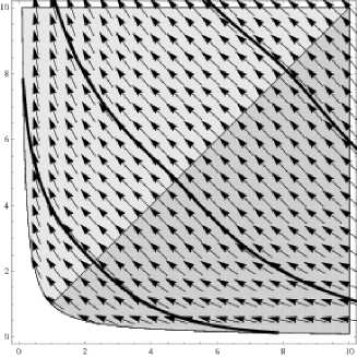
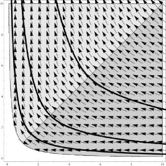
Figure 2. The vector fields $U_{1}/\|U_{1}\|$ and $U_{2}/\|U_{2}\|$, with some of their integral curves.

By construction, the trajectories of the integral curves of $U_{1}$ and $U_{2}$ are graphs of strictly decreasing functions, and hence they intersect $\partial_{+}\Sigma$ in at most one point. In addition, for every $Q=(x,y)\in\widetilde{\Omega}$, we have

• the connected components of the level curve $\mathcal{V}_{1}(x)=\Phi_{1}^{-1}(x)\cap\Sigma$ are contained in the intersection of a trajectory of $U_{1}$ with $\Sigma$.

• the connected components of the level curve $\mathcal{V}_{2}(y)=\Phi_{2}^{-1}(y)\cap\Sigma$ are contained in the intersection of a trajectory of $U_{2}$ with $\Sigma$.

We now prove the following.

Lemma 3.7.

The level curve $\mathcal{V}_{1}(x^{\prime})$ is connected, for every $Q^{\prime}=(x^{\prime},y^{\prime})\in\widetilde{\Omega}$.

Proof.

Consider the arcs $\partial_{+}\widetilde{\Omega}^{\prime}=\partial_{+}\widetilde{\Omega}\setminus\{Q_{1},Q_{3}\}$, $\partial_{-}\widetilde{\Omega}^{\prime}=\partial_{-}\widetilde{\Omega}\setminus\{Q_{1},Q_{2}\}$, $\partial_{+}\Sigma^{\prime}\!=\!\partial_{+}\Sigma\setminus\!\{V\}$ and $\partial_{-}\Sigma^{\prime}\!=\!\partial_{-}\Sigma\setminus\!\{V\}$. From the proof of Proposition 3.5, we know that the maps $\widehat{\Phi}|_{\partial_{+}\Sigma^{\prime}}:\partial_{+}\Sigma^{\prime}\to\partial_{+}\Omega^{\prime}$ and $\widehat{\Phi}|_{\partial_{-}\Sigma^{\prime}}:\partial_{-}\Sigma^{\prime}\to\partial_{-}\Omega^{\prime}$ are real-analytic diffeomorphisms. For every $Q^{\prime}=(x^{\prime},y^{\prime})\in\widetilde{\Omega}$, let $Q^{\prime}_{\pm}$ denote the intersections of $\partial_{\pm}\widetilde{\Omega}^{\prime}$ with the line $x=x^{\prime}$ and let $P^{\prime}_{+}=(a^{\prime}_{+},a^{\prime}_{+})$ and $P^{\prime}_{-}=(a^{\prime}_{-},1/a^{\prime}_{-})$ be the points of $\partial_{\pm}\Sigma^{\prime}$, such that $\widehat{\Phi}(P^{\prime}_{\pm})=Q^{\prime}_{\pm}$. Note that $\widehat{\Phi}_{1}^{-1}(x^{\prime})=\Phi_{1}^{-1}(x^{\prime})\cup\{P^{\prime}_{+},P^{\prime}_{-}\}$.

$\bullet$ First, we prove that $\widehat{\Phi}_{1}^{-1}(x^{\prime})$ is compact. By continuity, $\widehat{\Phi}_{1}^{-1}(x^{\prime})$ is closed. Suppose that $\widehat{\Phi}_{1}^{-1}(x^{\prime})$ is unbounded. Then, there is a sequence $\{P_{n}\}=\{(a_{n},b_{n})\}\subset\Phi_{1}^{-1}(x^{\prime})$, such that $\lim_{n\to\infty}a_{n}=+\infty$. By Lemma 3.6, $\{\Phi_{1}(P_{n})\}$ converges to $-1/2$. On the other hand, the points $P_{n}$ belong to $\mathcal{V}_{1}(x^{\prime})$, and hence $x^{\prime}$, which is the limit of the sequence $\{\Phi_{1}(P_{n})\}$, must be equal to $-1/2$. But this is absurd, since $(x^{\prime},y^{\prime})\in\widetilde{\Omega}$ and the abscissae of the points in $\widetilde{\Omega}$ are different from $-1/2$. This proves the compactness of $\widehat{\Phi}_{1}^{-1}(x^{\prime})$.

$\bullet$ Next, we prove that the points $P^{\prime}_{\pm}$ belong to the boundary of any connected component of the level curve $\mathcal{V}_{1}(x^{\prime})$. Let $C$ be a connected component of $\mathcal{V}_{1}(x^{\prime})$. We know that $C$ is the graph of a strictly decreasing function and that such a function is bounded, by the compactness of $\widehat{\Phi}_{1}^{-1}(x^{\prime})$. Since $C$ is an embedded curve, its boundary consists of two distinct points. On the other hand, $C\subset\Phi_{1}^{-1}(x^{\prime})\subset\widehat{\Phi}_{1}^{-1}(x^{\prime})=\Phi_{1}^{-1}(x^{\prime})\cup\{P^{\prime}_{+},P^{\prime}_{-}\}$. Using the fact that $\Phi_{1}^{-1}(x^{\prime})$ is an embedded curve, we have that $P^{\prime}_{+}$ and $P^{\prime}_{-}$ are the two boundary points of $C$.

$\bullet$ To complete the proof, we show that two connected components of the level curves intersect each other. The vector field $U_{1}$ does not vanishes at the point $P^{\prime}_{+}$ and $P^{\prime}_{+}$ belongs to the boundary of $C$. Therefore, $C$ is contained in the trajectory of $U_{1}$ passing through $P^{\prime}_{+}$. Choose local coordinates $(u,v)$ defined on a cubical open neighborhood $A$ of the point $P^{\prime}_{+}$, such that $U_{1}|_{A}=\partial_{u}$ and $v(P^{\prime}_{+})=0$. In these coordinates, the intersection $C\cap A$ consists of the points $P\in A$ such that $v(P)=0$ and $0<u(P)<\epsilon$, for some $\epsilon>0$. So, if $C$ and $C^{\prime}$ are two connected components of $\mathcal{V}_{1}(x^{\prime})$, there exist $\epsilon,\epsilon^{\prime}>0$, such that $C\cap A=\{P\in A\,:\,v(P)=0,\,0<u(P)<\epsilon\}$ and $C^{\prime}\cap A=\{P\in A\,:\,v(P)=0,\,0<u(P)<\epsilon^{\prime}\}$. This implies that $C\cap C^{\prime}\neq\emptyset$. ∎

A similar result also holds for the other family of level curves.

Lemma 3.8.

The level curves $\mathcal{V}_{2}(y^{\prime})$ are connected, for every $Q^{\prime}=(x^{\prime},y^{\prime})\in\widetilde{\Omega}$.

Proof.

Let $C$ be any connected component of $\mathcal{V}_{2}(y^{\prime})$. Fix $(a,b)\in C$ and take a strictly decreasing function $u:I\to\mathbb{R}$ whose graph coincides with $C$. Such a function is defined on an open interval $I$ of the form $(a-\epsilon_{1},a+\epsilon_{2})$, where $\epsilon_{1},\epsilon_{2}>0$ and $a-\epsilon_{1}>1$. Let $\{a_{n}\}\subset(a-\epsilon_{1},a)$ be a decreasing sequence, such that $\lim_{n\to\infty}a_{n}=a^{*}=a-\epsilon_{1}$. By construction, $\{u(a_{n})\}$ is an increasing sequence and $(a_{n},u(a_{n}))\in C\subset\Sigma$, for every $n$. In particular, $0<a_{n}^{-1}<u(a_{n})<a_{n}<a$, which implies that $\{u(a_{n})\}$ is bounded. By possibly taking a subsequence, we may assume that $\{u(a_{n})\}$ converges to a limit point $b^{*}$. Since $\{(a_{n},u(a_{n}))\}$ converges to $(a^{*},b^{*})$, the point $(a^{*},b^{*})$ belongs to $\partial C\cap\bar{\Sigma}$.

$\bullet$ We prove that $(a^{*},b^{*})$ is an element of $\partial\Sigma$. By contradiction, suppose that $(a^{*},b^{*})\in\Sigma$. Then, $C$ is contained in the trajectory, $C^{\prime}$, of the vector field $U_{2}|_{\Sigma}$ passing through $(a^{*},b^{*})$. By definition, $(a^{*},b^{*})\in C^{\prime}$ and $(a^{*},b^{*})\notin C$. Therefore, $C^{\prime}$ is a connected subset of $\mathcal{V}_{2}(y^{\prime})$ which contains properly $C$. This is absurd since $C$ is a connected component of $\mathcal{V}_{2}(y^{\prime})$.

By construction, since $1/a^{*}<u(a_{n})$ and ${u(a_{n})}$ is an increasing sequence, $b^{*}\neq 1/a^{*}$. This shows that $(a^{*},b^{*})$ does not belong to $\partial_{-}\Sigma$. Therefore, $(a^{*},b^{*})$ is an element of $\partial_{+}\Sigma$ and hence $b^{*}=a^{*}$ and $a^{*}>1$. The point $(a^{*},a^{*})$ is independent of the choice of the connected component. Otherwise, the restriction of $\widetilde{\Phi}$ to $\partial_{+}\Sigma$ could not be injective. We are now in the same situation as in the last part of the proof of the previous lemma, i.e., the point $(a^{*},a^{*})$ belongs to the boundary of any connected component of the level curve $\mathcal{V}_{2}(y^{\prime})$. By arguing as above, we deduce the result. ∎

We are now ready to prove the last ingredient for the proof of Theorem 3.1.

Proposition 3.9.

The mapping $\Phi$ is injective.

Proof.

It suffices to show that $\#\left(\mathcal{V}_{1}(x)\cap\mathcal{V}_{2}(y)\right)=1$, for every $(x,y)\in\widetilde{\Omega}$. By contradiction, suppose the existence of $(x,y)\in\widetilde{\Omega}$, such that $\sharp(\mathcal{V}_{1}(x)\cap\mathcal{V}_{2}(y))>1$. Let $(a,b)$ and $(a_{1},b_{1})$ be two distinct elements of $\Sigma$, such that $\Phi(a_{1},b_{1})$ $=$ $\Phi(a,b)$ $=$ $(x,y)$. From the above discussions, we know that the level curves $\mathcal{V}_{1}(x)$ and $\mathcal{V}_{2}(y)$ are connected and graphs of two strictly decreasing functions, denoted by $u$ and $v$, respectively. The domain of definition is an open interval $I\subset(1,+\infty)$, containing $a$ and $a_{1}$. By construction, $u(a)=v(a)=b$, $u(a_{1})=v(a_{1})=b_{1}$, with $a\neq a_{1}$. On the other hand, $\mathcal{V}_{1}(x)$ and $\mathcal{V}_{2}(y)$ are contained in the trajectories of the vector fields $U_{1}$ and $U_{2}$, respectively. From this, we have

$$u^{\prime}(t)=-\frac{\partial_{a}\Phi_{1}}{\partial_{b}\Phi_{1}}\bigg{|}_{(t,u(t))},\quad v^{\prime}(t)=-\frac{\partial_{a}\Phi_{2}}{\partial_{b}\Phi_{2}}\bigg{|}_{(t,v(t))},\quad\forall t\in I.$$

Now, Proposition 3.2 and Proposition 3.4 imply

(3.7) $$\frac{\partial_{a}\Phi_{1}}{\partial_{b}\Phi_{1}}\bigg{|}_{(\alpha,\beta)}-\frac{\partial_{a}\Phi_{2}}{\partial_{b}\Phi_{2}}\bigg{|}_{(\alpha,\beta)}>0,\quad\forall(\alpha,\beta)\in\Sigma.$$

Then, the function $h=v-u$ satisfies $h(a)=h(a_{1})=0$, $h^{\prime}(a)>0$ and $h^{\prime}(a_{1})>0$. This implies the existence of $a_{2}\in I$, different from $a$ and $a_{1}$, such that $h(a_{2})=0$ and $h^{\prime}(a_{2})\leq 0$. Consequently, the Jacobian of $\Phi$ is non positive at $(a_{2},b_{2})$ $=$ $(a_{2},u(a_{2}))=(a_{2},v(a_{2}))\in\Sigma$, contrary to Proposition 3.4. ∎

4. The proof of Theorem B

Theorem B asserts that any Möbius class of conformal strings is represented by a model conformal string. We will begin the proof by describing the model strings.

4.1. The symmetrical configuration of a string

We have just proved that the Möbius classes of conformal strings are in one-to-one correspondence with the moduli, i.e., the elements of the countable set

(4.1) $$\Omega_{*}=\left\{(q_{1},q_{2})\in\mathbb{Q}^{2}\,:\,1/2<q_{1}<1/\sqrt{2},\,q_{2}>0,\,q_{1}^{2}+q_{2}^{2}<1/2\right\}.$$

Thus, for every $q=(q_{1},q_{2})\in\Omega_{*}$, there is a unique $(a,b)\in\Sigma$ such that $\Phi_{1}(a,b)=-q_{1}$ and $\Phi_{2}(a,b)=q_{2}$. For every $(q_{1},q_{2})\in\Omega_{*}$, let

(4.2) $$\Theta_{1}(t)=\int_{0}^{t}\frac{\mu}{\mu^{2}-k(u)^{2}}du,\quad\Theta_{2}(t)=\int_{0}^{t}\frac{\upsilon}{\upsilon^{2}-k(u)^{2}}du$$

and

(4.3) $$r(t)=\sqrt{\mu^{2}-\upsilon^{2}}k(t)+\upsilon\sqrt{\mu^{2}-k(t)^{2}}\cos\Theta_{1}(t),$$

where $a,b$ are the parameters of $q$ and $k$, $\mu$, $\upsilon$ stand for $k_{a,b}$, $\mu(a,b)$ and $\upsilon(a,b)$, respectively. Note that $(q_{1},q_{2})$ and $(a,b)$ are related by

(4.4) $$q_{1}=\frac{1}{2\pi}\int_{0}^{\omega}\Theta_{1}^{\prime}(t)dt,\quad q_{2}=-\frac{1}{2\pi}\int_{0}^{\omega}\Theta_{2}^{\prime}(t)dt,$$

where $\omega=\omega(a,b)$ is the minimal period of $k$.

Definition 4.1.

The symmetrical configuration of the conformal strings with modulus $q=(q_{1},q_{2})$ is the parametrized curve $\gamma_{q}=(x,y,z):\mathbb{R}\to\mathbb{R}^{3}$, defined by

(4.5) $$\begin{cases}x(t)=\frac{\sqrt{2}}{r(t)}\mu\sqrt{k(t)^{2}-\upsilon^{2}}\cos\Theta_{2}(t),\\ y(t)=\frac{\sqrt{2}}{r(t)}\mu\sqrt{k(t)^{2}-\upsilon^{2}}\sin\Theta_{2}(t),\\ z(t)=\frac{\sqrt{2}}{r(t)}\upsilon\sqrt{\mu^{2}-k(t)^{2}}\sin\Theta_{1}(t).\\ \end{cases}$$

Theorem B is now a direct consequence of the following.

Theorem 4.1.

Let $q=(q_{1},q_{2})$ be any element of $\Omega_{*}$ and $(a,b)\in\Sigma_{*}$ be the corresponding parameters. Any conformal string with parameters $(a,b)$ is conformally equivalent to the symmetrical configuration $\gamma_{q}$.

Proof.

Consider the unique conformal parametrization $\gamma:\mathbb{R}\to\mathbb{R}^{3}$ of a conformal string with parameters $a$, $b$ whose Vessiot frame $\mathrm{F}$ satisfies the initial condition $\mathrm{F}(0)=\mathrm{Id}$. It suffices to prove that $\gamma$ is conformally equivalent to $\gamma_{q}$. By Lemma 2.4, the canonical lift $\Gamma:\mathbb{R}\to\mathcal{L}_{+}$ of $\gamma$ takes the form $\tilde{Y}W$, where $\tilde{Y}\in GL(5,\mathbb{C})$ and $W={}^{t}\!(w_{0},\dots,w_{4})$ is the $\mathbb{C}^{5}$-valued map defined by

(4.6) $$w_{0} =k,\quad w_{1}=\sqrt{\mu^{2}-k^{2}}e^{i\Theta_{1}(t)},\quad w_{2}=\sqrt{\mu^{2}-k^{2}}e^{-i\Theta_{1}(t)},$$

$$w_{3} =\sqrt{\upsilon^{2}-k^{2}}e^{i\Theta_{2}(t)},\quad w_{4}=\sqrt{\upsilon^{2}-k^{2}}e^{-i\Theta_{2}(t)},$$

On the other hand, the curve $\widetilde{\Gamma}={}^{t}\!(\widetilde{\gamma}_{0},\dots,\widetilde{\gamma}_{4}):\mathbb{R}\to\mathcal{L}_{+}$, defined by

(4.7) $$\begin{cases}\widetilde{\gamma}_{0}(t)=\frac{1}{\sqrt{2}}\left(\sqrt{\mu^{2}-\upsilon^{2}}k(t)-\upsilon\sqrt{\mu^{2}-k(t)^{2}}\cos\Theta_{1}(t)\right),\\ \widetilde{\gamma}_{1}(t)=\mu\sqrt{k(t)^{2}-\upsilon^{2}}\cos\Theta_{2}(t),\\ \widetilde{\gamma}_{2}(t)=\mu\sqrt{k(t)^{2}-\upsilon^{2}}\sin\Theta_{2}(t),\\ \widetilde{\gamma}_{3}(t)=\upsilon\sqrt{\mu^{2}-k(t)^{2}}\sin\Theta_{1}(t),\\ \widetilde{\gamma}_{4}(t)=\frac{1}{\sqrt{2}}\left(\sqrt{\mu^{2}-\upsilon^{2}}k(t)+\upsilon\sqrt{\mu^{2}-k(t)^{2}}\cos\Theta_{1}(t)\right),\end{cases}$$

is a null lift of $\gamma_{q}$. From (4.6) and (4.7), it follows that $W=\mathrm{Z}\widetilde{\Gamma}$, for some $\mathrm{Z}\in GL(5,\mathbb{C})$. Consequently, $\Gamma=\mathrm{L}\widetilde{\Gamma}$, for a suitable $\mathrm{L}\in GL(5,\mathbb{C})$, which yields $\mathrm{F}=\mathrm{L}\mathrm{F}_{q}$, where $\mathrm{F}_{q}$ is the Vessiot frame along $\gamma_{q}$. Thus $\mathrm{L}\in G_{+}$, which implies that $\gamma$ and $\gamma_{q}$ are equivalent to each other. ∎

Remark 4.

The map $\Phi$ can be inverted by numerical methods. Once we know the parameters $a$ and $b$ which correspond to the modulus $q$, we can use (4.5) to find the explicit parametrization of the symmetrical configuration $\gamma_{q}$.

5. The proof of Theorem C

Let $\Omega_{*}$ be the countable set introduced in (4.1). For every $q=(q_{1},q_{2})\in\Omega_{*}$, let $q_{1}=m_{1}/n_{1}$ and $q_{2}=m_{2}/n_{2}$, with $(m_{1},n_{1})=(m_{2},n_{2})=1$. Let $n$ denote the least common multiple of $n_{1}$ and $n_{2}$. Then, $n=h_{1}n_{1}$ and $n=h_{2}n_{2}$, where $h_{1}$ and $h_{2}$ are two positive coprime integers. Let $\gamma_{q}$ be the symmetrical configuration corresponding to $q$ (cf. Definition 4.1). We are now ready to prove Theorem C asserting that (1) $n$ is the order of the symmetry group of $\gamma_{q}$ and (2) $m_{1}h_{1}$ and $m_{2}h_{2}$ are, respectively, the linking numbers of $\gamma_{q}$ with the Clifford circle $\mathcal{C}=\left\{(x,y,0)\in\mathbb{R}^{3}:x^{2}+y^{2}=2\right\}$ and with the $z$-axis.

Proof of Theorem C.

The curve $\gamma_{q}$ is a real-analytic closed curve with positive chirality (cf. Section 1.2, Definition 1.1). Therefore, the symmetry group of $\gamma_{q}$ is generated by the monodromy of $\gamma_{q}$. By construction, the canonical null lift $\Gamma:\mathbb{R}\to\mathcal{L}_{+}$ is as in (4.7) and the first conformal curvature is a strictly positive periodic function, with minimal period $\omega$. Using (4.7), we find $\Gamma_{q}(t+\omega)=R(2\pi q_{2},2\pi q_{1})\Gamma_{q}(t)$, where $R(2\pi q_{2},2\pi q_{1})$ is as in (1.6). Therefore, $R(2\pi q_{2},2\pi q_{1})$ is the monodromy of $\gamma_{q}$. This implies that the symmetry group of $\gamma_{q}$ is generated by $R(2\pi q_{2},2\pi q_{1})$. Let $[z]$ denote the $z$-axis with the downward orientation induced by the parametrization $\alpha(s)=(0,0,-s)$, and let $[\mathcal{C}]$ be the Clifford circle equipped with the orientation induced by the rational parametrization

$$\beta:t\in\mathbb{R}\mapsto(-\sqrt{2}(t^{2}-2)/(t^{2}+2),4t/(2+t^{2}),0)\in\mathbb{R}^{3}.$$

Now we compute the Gauss linking integrals $\mathrm{lk}(\gamma_{q},[z])$ and $\mathrm{lk}(\gamma_{q},[\mathcal{C}])$. If $\gamma_{q}(t)=(x(t),y(t),z(t))$, the Gauss linking integral $\mathrm{lk}(\gamma_{q},[z])$ is given by

$$\begin{split}\mathrm{lk}(\gamma_{q},[z])&=\frac{1}{4\pi}\int_{[\gamma_{q}]}\int_{z}\left\langle\frac{\gamma_{q}-\alpha}{\|\gamma_{q}-\alpha\|^{3}},d\gamma_{q}\times d\alpha\right\rangle\\ &=-\frac{1}{4\pi}\int_{0}^{n\omega}\left(\int_{-\infty}^{+\infty}\left(\frac{x(t)y^{\prime}(t)-x^{\prime}(t)y(t)}{\left[x(t)^{2}+y(t)^{2}+(z(t)+s)^{2}\right]^{3/2}}\right)ds\right)dt\\ &=-\frac{1}{2\pi}\int_{0}^{n\omega}\frac{x(t)y^{\prime}(t)-x^{\prime}(t)y(t)}{x(t)^{2}+y(t)^{2}}dt\\ &=-\frac{n}{2\pi}\int_{0}^{\omega}\Theta_{2}^{\prime}(t)dt=n\Phi_{2}=nq_{2}=h_{2}m_{2}.\end{split}$$

To compute the linking integral of $\gamma_{q}$ with the Clifford circle we consider the orientation-preserving conformal involution

(5.1) $$\Psi:(x,y,z)\in\mathbb{R}^{3} \mapsto\frac{1}{x^{2}+y^{2}+z^{2}+2\sqrt{2}x+2}$$

$$\quad\times\left(x^{2}+y^{2}+z^{2}+2\sqrt{2},4z,4y\right)\in\mathbb{R}^{3}.$$

This map takes $(-\sqrt{2},0,0)$ to the point at infinity and exchanges the roles of the two axes of symmetry, i.e., $\Phi\circ\beta=-\alpha$. A direct computation shows that the parametric equations of $\gamma_{*}:=\Phi\circ\gamma_{q}$ are

$$\begin{cases}x_{*}(t)=\frac{\sqrt{2}}{r^{*}(t)}\upsilon\sqrt{\mu^{2}-k(t)^{2}}\cos\Theta_{1}(t),\\ y_{*}(t)=\frac{\sqrt{2}}{r^{*}(t)}\upsilon\sqrt{\mu^{2}-k(t)^{2}}\sin\Theta_{1}(t),\\ z_{*}(t)=\frac{\sqrt{2}}{r^{*}(t)}\mu\sqrt{k(t)^{2}-\upsilon^{2}}\sin\Theta_{2}(t),\end{cases}$$

where $r^{*}(t)=\sqrt{\mu^{2}-\upsilon^{2}}k(t)+\mu\sqrt{k(t)^{2}-\upsilon}\cos\Theta_{2}(t)$. We then have

$$\begin{split}\mathrm{lk}(\gamma_{q},[\mathcal{C}])&=-\mathrm{lk}(\gamma_{*},[z])=-\frac{1}{4\pi}\int_{[\gamma_{*}]}\int_{z}\left\langle\frac{\gamma_{*}-\alpha}{\|\gamma_{*}-\alpha\|^{3}},d\gamma_{*}\times d\alpha\right\rangle\\ &=\frac{1}{4\pi}\int_{0}^{n\omega}\left(\int_{-\infty}^{+\infty}\left(\frac{x_{*}(t)y_{*}^{\prime}(t)-x_{*}^{\prime}(t)y_{*}(t)}{\left[x_{*}(t)^{2}+y_{*}(t)^{2}+(z_{*}(t)+s)^{2}\right]^{3/2}}\right)ds\right)dt\\ &=\frac{1}{2\pi}\int_{0}^{n\omega}\frac{x_{*}(t)y_{*}^{\prime}(t)-x_{*}^{\prime}(t)y_{*}(t)}{x_{*}(t)^{2}+y_{*}(t)^{2}}dt\\ &=\frac{n}{2\pi}\int_{0}^{\omega}\Theta_{1}^{\prime}(t)dt=-n\Phi_{1}=nq_{1}=h_{1}m_{1},\end{split}$$

which yields the required result. ∎

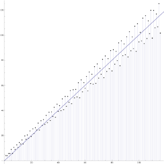
Figure 3. The graph of the function $4\sqrt{\varrho(n)}$, $5\leq n\leq 120$.

6. Final remarks and examples

In this section we discuss some examples and comment on some numerical experiments carried out with the software Mathematica.

6.1. Euclidean and Clifford symmetries

Let $\gamma$ be the symmetrical configuration with modulus $q=(q_{1},q_{2})$. Then, $E(q_{1},q_{2})=R(2\pi q_{2},2\pi q_{1})^{n_{1}}$ is the Euclidean rotation of angle $2\pi m_{2}n_{1}/n_{2}$ around the $z$-axis. The subgroup of order $h_{1}$ generated by $E(q_{1},q_{2})$ is the Euclidean symmetry group of the symmetrical configuration. Similarly, $C(q_{1},q_{2})=R(2\pi q_{2},2\pi q_{1})^{n_{2}}$ is the toroidal rotation of angle $2\pi m_{1}n_{2}/n_{1}$ around the Clifford circle. The cyclic subgroup of order $h_{2}$ generated by $C(q_{1},q_{2})$ is the Clifford symmetry group of the symmetrical configuration. Denoting by $\omega$ the conformal wavelength of $\gamma$, the arc $[\gamma]_{0}=\gamma([0,\omega))\subset[\gamma]$ is the fundamental domain of the string and the trajectory $[\gamma]$ is obtained from $[\gamma]_{0}$ via $G_{\gamma}$, i.e., $[\gamma]=\bigcup_{A\in G_{\gamma}}A\cdot[\gamma]_{0}$.

6.2. Quantum numbers

The symmetrical configurations are labeled by three quantum numbers: the order of the symmetry group and the linking numbers with the Clifford circle and the $z$-axis. We use the notation $|n,\ell_{1},\ell_{2}>$ for the symmetrical configuration with a symmetry group of order $n$ and linking numbers $\mathrm{lk}(\gamma,[\mathcal{C}])=\ell_{1}$ and $\mathrm{lk}(\gamma,[z])=\ell_{2}$, respectively. Let $\varrho(n)$ be the cardinality of the set of the symmetrical configurations with index of symmetry $n$. There are no symmetrical configurations with $n=1,2,3,4$. Figure 3 reproduces the graph of the function $4\sqrt{\varrho}$, for $5\leq n\leq 120$. This suggest that $\varrho$ has an asymptotic quadratic growth.

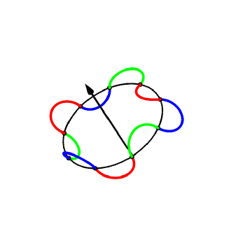
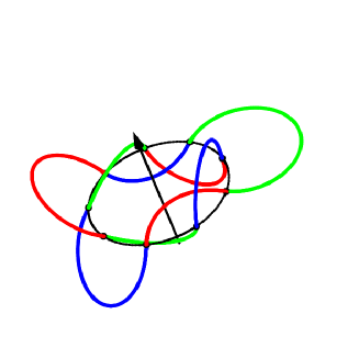
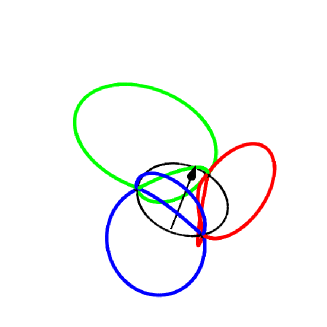
Figure 4. Symmetrical configurations $|9,5,1>$, $|9,5,2>$, and $|9,5,3>$, respectively.

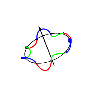
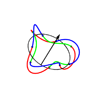
Figure 5. The symmetrical configurations $|9,6,1>$ and $|9,6,2>$, respectively.

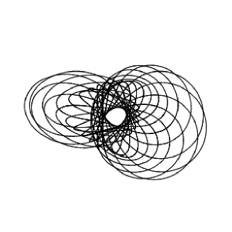
Figure 6. The symmetrical configuration $|63,37,24>$.

Example 2.

In this final example, we consider the symmetrical configurations with $n=9$. This set consists of five elements: $|9,5,1>$, $|9,5,2>$, $|9,5,3>$, $|9,6,1>$, and $|9,6,2>$. The moduli of these strings are $(5/9,1/9)$, $(5/9,2/9)$, $(5/9,1/3)$, $(2/3,1/9)$, and $(2/3,2/9)$, respectively. The Euclidean and the Clifford symmetry subgroups of the first two strings are trivial. The Euclidean symmetry group of the third string is trivial, while the Clifford symmetry group has order 3 (see Figure 4). The fourth and fifth strings have an Euclidean symmetry group of order 3 and have no non-trivial Clifford symmetries (see Figure 5). The invariants $a$, $b$ and the conformal wavelength $\omega$ can be tabulated against the quantum numbers $n$, $\ell_{1}$ and $\ell_{2}$. For instance, the values of the natural parameters $a$, $b$ and those of the conformal wavelength $\omega$ of the stings with $n=9$ are

$$<a|9,5,1> \approx 18.6403,\quad<b|9,5,1>\approx 0.06069,\quad<\omega|9,5,1>\approx 1.96996,$$

$$<a|9,5,2> \approx 16.9699\quad<b|9,5,2>\approx 0.09982,\quad<\omega|9,5,2>\approx 1.92188,$$

$$<a|9,5,3> \approx 13.3269,\quad<b|9,5,3>\approx 0.29125,\quad<\omega|9,5,3>\approx 1.81376,$$

$$<a|9,6,1> \approx 2.6203,\quad<b|9,6,1>\approx 0.42577,\quad<\omega|9,6,1>\approx 2.90618,$$

$$<a|9,6,2> \approx 1.7209,\quad<b|9,6,2>\approx 0.90777,\quad<\omega|9,6,2>\approx 2.79219.$$

The shape of the strings becomes more complicated when $n$, $\ell_{1}$ and $\ell_{2}$ increase, see for instance Figure 6, where the symmetrical configuration with $n=63$, $\ell_{1}=37$ and $\ell_{2}=24$ is reproduced. This string has no non-trivial Euclidean symmetries and the subgroup of its Clifford symmetries has order $3$.

References

- [1] S. Bryson, M. H. Freedman, Z.-X. He, and Z. Wang, Möbius invariance of knot energy, Bull. Amer. Math. Soc. (N.S.) 28 (1993), no. 1, 99–103.
- [2] F. E. Burstall and D. M. J. Calderbank, Conformal submanifold geometry I–III, arXiv:1006.5700 [math.DG].
- [3] P. F. Byrd and M. D. Friedman, Handbook of elliptic integrals for engineers and physicists, Springer-Verlag, Berlin, Göttingen, Heidelberg, 1954.
- [4] G. Cairns, R. W. Sharpe, and L. Webb, Conformal invariants for curves and surfaces in three dimensional space forms, Rocky Mountain J. Math. 24 (1994), 933–954.
- [5] K.-S. Chou and C.-Z. Qu, Integrable equations arising from motions of plane curves. II, J. Nonlinear Sci. 13 (2003), 487–517.
- [6] B. A. Dubrovin, A. T. Fomenko, and S. P. Novikov, Modern geometry–methods and applications. Part I, 2nd edn., GTM 93, Springer-Verlag, New York, 1992.
- [7] A. Dzhalilov, E. Musso, and L. Nicolodi, Conformal geometry of timelike curves in the (1+2)-Einstein universe, Nonlinear Anal. 143 (2016), 224–255.
- [8] M. Eastwood and G. Marí-Beffa, Geometric Poisson brackets on Grassmannians and conformal spheres, Proc. Roy. Soc. Edinburgh Sect. A 142 (2012), no. 3, 525–561.
- [9] A. Fialkow, The conformal theory of curves, Trans. Amer. Math. Soc. 51 (1942), 435–501.
- [10] A. T. Fomenko and V. V. Trofimov, Geometric and algebraic mechanisms of the integrability of Hamiltonian systems on homogeneous spaces and Lie algebras, Dynamical Systems, Vol. 7, Springer-Verlag, 1994.
- [11] M. H. Freedman, Z.-X. He, and Z. Wang, Möbius energy of knots and unknots, Ann. of Math. (2) 139 (1994), no. 1, 1–50.
- [12] J. D. Grant and E. Musso, Coisotropic variational problems, J. Geom. Phys. 50 (2004), 303–338.
- [13] P. A. Griffiths, Exterior differential systems and the calculus of variations, Progress in Mathematics 25, Birkhäuser, Boston, 1982.
- [14] V. Guillemin and S. Sternberg, Symplectic techniques in Physics, Cambridge University Press, Cambridge, 1990.
- [15] U. Hertrich-Jeromin, Introduction to Möbius differential geometry, London Mathematical Society Lecture Note Series 300, Cambridge University Press, 2003.
- [16] G. R. Jensen, E. Musso, and L. Nicolodi, Surfaces in classical geometries. A treatment by moving frames, Universitext, Springer, Cham, 2016.
- [17] B. Jovanovic, Noncommutative integrability and action-angle variables in contact geometry, J. Symplectic Geom. 10 (2012), no. 4, 535–561.
- [18] R. Langevin and J. O’Hara, Conformally invariant energies of knots, J. Inst. Math. Jussieu 4 (2005), no. 2, 219–280.
- [19] R. Langevin and J. O’Hara, Conformal arc-length as -dimensional length of the set of osculating circles, Comment. Math. Helv. 85 (2010), no. 2, 273–312.
- [20] D. F. Lawden, Elliptic functions and applications, Series in Applied Mathematical Science 80, Springer-Verlag, New York, 1989.
- [21] H. Liebmann, Beiträge zur Inversionsgeometrie der Kurven, Münchener Berichte, 1923.
- [22] M. Magliaro, L. Mari, and M. Rigoli, On the geometry of curves and conformal geodesics in the Möbius space, Ann. Global Anal. Geom. 40 (2011), 133–165.
- [23] V. O. Manturov, Knot theory, Chapman & Hall/CRC Press, Boca Raton, 2004.
- [24] A. Messiah, Quantum mechanics, Dover Publications, Inc., Mineola, NY, 2003.
- [25] A. Montesinos Amilibia, M. C. Romero Fuster, and E. Sanabria, Conformal curvatures of curves in , Indag. Math. (N.S.) 12 (2001), 369–382.
- [26] E. Musso, The conformal arclength functional, Math. Nachr. 165 (1994), 107–131.
- [27] E. Musso, Closed trajectories of the conformal arclength functional, Journal of Physics: Conference Series 410 (2013), 012031.
- [28] E. Musso and L. Nicolodi, Reduction for the projective arclength functional, Forum Math. 17 (2005), 569–590.
- [29] E. Musso and L. Nicolodi, Closed trajectories of a particle model on null curves in anti-de Sitter -space, Class. Quantum Grav. 24 (2007), 5401–5411.
- [30] E. Musso and L. Nicolodi, Reduction for constrained variational problems on -dimensional null curves, SIAM J. Control Optim. 47 (2008), 1399–1414.
- [31] E. Musso and L. Nicolodi, Invariant signatures of closed planar curves, J. Math. Imaging Vision 35 (2009), 68–85.
- [32] E. Musso and L. Nicolodi, Hamiltonian flows on null curves, Nonlinearity 23 (2010), 2117–2129.
- [33] P. Ortega and T. Ratiu, Moment maps and hamiltonian reductions, Progress in Mathematics, 222, Birkhäuser, Boston, 2004.
- [34] S. Ourselin and M. A. Styner (eds.), Medical Imaging 2014: Image Processing, Proceedings of SPIE, vol. 9034; DOI:10.1117/12.2052780.
- [35] C. Schiemangk and R. Sulanke, Submanifolds of the Möbius space, Math. Nachr. 96 (1980), 165–183.
- [36] R. Sulanke, Submanifolds of the Möbius space II, Frenet formula and curves of constant curvatures, Math. Nachr. 100 (1981), 235–257.
- [37] T. Takasu, Differentialgeometrien in den Kugelräumen. Band I. Konforme Differentialkugelgeometrie von Liouville und Möbius, Maruzen, Tokyo, 1938.
- [38] E. Vessiot, Contribution à la géométrie conforme. Enveloppes de sphères et courbes gauches, J. École Polytechnique 25 (1925), 43–91.
- [39] E. W. Weisstein, Elliptic Integral of the Third Kind, from: MathWorld — A Wolfram Web Resource. http://mathworld.wolfram.com/EllipticIntegraloftheThirdKind.html.